Uniqueness Results for Bodies of Constant Width in the Hyperbolic Plane
Abstract.
Following Santaló’s approach, we prove several characterizations of a disc among bodies of constant width, constant projections lengths, or constant section lengths on given families of geodesics.
1. Introduction
The reconstruction of a convex body from quantitative lower dimensional information (such as the areas of sections or projections) is one of the main problems in geometric tomography. One of the main results in this area is Aleksandrov’s Theorem. He proved that an origin-symmetric convex body in is uniquely determined by the -dimensional volumes of its projections (see [5, Theorem 3.3.6]). The focus of the current note is the study of reconstruction problems in the hyperbolic plane .
The question of uniqueness plays a central role in the study of reconstruction, i.e., do there exist two bodies and with the same projections (or sections) on a given family of geodesic lines? Often, it is assumed that one of the bodies is a disc, and the problem is stated as:
Does there exist a body with constant projections or sections on a given family of geodesics, which is not a disc?
The width of a smooth convex body in the hyperbolic plane is defined to be its projection lengths on the family of normal lines (see the precise definition in Section 2). An important difference between the geometry in the Euclidean and the hyperbolic plane is that, while the concepts of width o f a body and its projections lengths coincide in the Euclidean setting, they capture different information in the hyperbolic one. For example, any Euclidean planar body of constant width has constant projection lengths on every line, but this no longer holds in the hyperbolic plane, see Remark 4.3.
Bodies of constant width in hyperbolic spaces have been studied in the literature, and several analogues of Euclidean results have been established (see e.g. [1], [3], [4], [7], [8], [10] and references therein). Problems about sections of convex bodies in hyperbolic spaces (related to the Busemann-Petty problem) have been studied in [6], [11]. In this paper we study bodies of constant width by their sections or projections on all lines through a given point. In particular, we consider the following four classes of convex bodies in :
-
origin-symmetric bodies.
-
Constant width bodies.
-
Bodies of constant projection lengths on all lines through a point.
-
Bodies of constant sections lengths on all lines through a point.
We show that the disc in is uniquely characterized by any two of the above properties. Some of these characterizations follow immediately from the definitions (e.g. origin symmetry plus constant section lengths), but are included for completeness. Our main results are:
Theorem 4.1. Let be a -smooth convex body. If is origin-symmetric and has constant width, then is a disc.
Theorem 4.4. Let be a -smooth convex body, containing the origin in its interior. If is a body of constant width and all projections of on the geodesics passing through the origin have constant length, then is a disc.
Theorem 4.4 is a result that has no Euclidean analog, since in having constant width and constant projection lengths is the same property. A version of Theorem 4.1 was proven in [7], where the authors use a different definition for width than the one we present below.
The paper is organized as follows. In Section 2 we introduce the needed definitions and notation. In Section 3 we collect several auxiliary lemmas that will be needed for the main results. In Section 4 we prove Theorems 4.1 and 4.4. We also include a unique reconstruction result for general convex bodies from projection lengths on two families of geodesics. Finally, the Appendix contains some computations for the hyperbolic Reuleaux triangle.
Acknowledgments: We would like to thank Dmitry Ryabogin and Vlad Yaskin for many fruitful discussions about this paper, in particular for the result in Section 4.2.
2. Definitions and Notation
Throughout the paper, we work interchangeably in the Poincaré disc model and the Poincaré upper half-plane model of the hyperbolic plane . We refer to the book [2, Volume 2, Chapter 19] for definitions and properties of the hyperbolic plane and its various models. Here we recall some basic facts: Given two points , there is a unique geodesic line joining them. Also, both models are conformal, and hence angles and the notion of perpendicularity are defined as in the Euclidean setting. In particular, given a point on a geodesic and an angle there exists a unique geodesic passing through and forming an angle with . We use the disc model when studying centrally symmetric bodies, while the upper half-plane model is well suited to the geometry of the proof of Lemma 4.2. In only one instance (Lemma 3.1) we use the Beltrami-Klein disc model, in which geodesics are straight lines; this allows us to directly use the corresponding Euclidean property. For more detail on the Beltrami-Klein disc model see [9].
A body is a compact set that is equal to the closure of its non-empty interior. A body is called convex if its boundary cannot be intersected by a geodesic in more than two points (with the exception that an arc of a geodesic may be part of the boundary). Any geodesic that has only a common point with or with a complete arc of is called a supporting geodesic of . We will often assume that the boundary of is -smooth and contains no geodesic segments.
Given two points , we denote by the unique geodesic segment joining them, and by the length of this segment. Given a geodesic in and a point , we denote by the perpendicular (or normal) geodesic to passing through . In particular, if is -smooth, given and letting be a supporting geodesic of at , we will write (instead of ) for the normal geodesic to at the point . The set of all normal geodesics to will be called the normal field of . A geodesic is called a double normal geodesic of if it intersects perpendicularly at two points.
The projection of the body onto a geodesic is defined as
Several non-equivalent definitions of width have been introduced in previous works (see [10] and [7]). We follow Santaló’s definition [10]. Given and the normal geodesic , let be another supporting geodesic of which is also orthogonal to . If is the point of intersection of and , we define the width of at by (see Figure 1, left). We note that the width of at equals the length of the projection , but it need not equal the length of the projection of on another geodesic perpendicular to (such as the geodesic passing through in Figure 1, right). Thus, we see that in contrast with the Euclidean situation, there is no natural way of defining the support function of a convex body in the hyperbolic setting.

With this definition, bodies of constant width are, like in the Euclidean case, precisely those for which every normal geodesic is double normal (i.e., for each , the corresponding point is also on ; see [10, pg. 410] for details). A body of constant width in has constant projection lengths on every line, but in this is not the case; in fact one can always find a geodesic on which has an arbitrarily small projection length.
A point is said to be equichordal to a body if all intersections of by lines through have equal lengths. The set of all lines passing through a fixed point will be denoted by . Given a geodesic , we denote by the set of all the geodesics perpendicular to .
Let be a convex body in the Poincaré disc model of , containing the origin in its interior. We say that is origin-symmetric if for every , we have .
3. Auxiliary Lemmas
In this section we state some basic metric facts regarding convex bodies and their orthogonal projections in the hyperbolic plane. The first one is the characterization of a hyperbolic convex body as the intersection of all half-planes containing it. We prove this using the Beltrami-Klein disc model, where the geodesics are the chords of the (open) disc , and thus the compact convex sets in correspond to the compact convex subsets of the open disc in .
Lemma 3.1.
Let be a convex body. Then equals the intersection of all the half-planes containing it.
Proof.
In the Beltrami-Klein disc model, for any supporting half-plane we denote by the (unique) half-plane of such that .
where the third equality holds since in the Euclidean plane, a convex sets equals the intersection of all containing half-planes. ∎
Remark 3.2.
The projection of a centrally symmetric convex body is symmetric, hence knowing the lengths of the projections on geodesic from determines the half-planes containing . Without central symmetry the lengths of projections on do not determine the body, as seen in the following example.
Example 3.3.
We present two non-congruent polygons , that have equal lengths of projections on . We will follow the construction in the Euclidean plane from [5, Theorem 3.3.15]. In Figure 2, the polygons and are presented in the upper half-plane, and the origin from the Beltrami-Klein disc is mapped to the point on the upper half-plane.


The lengths of the projections of and on each geodesic in coincide. Indeed, let be the geodesic passing through and , and the one passing through and . The two bodies are reflections of each other in the region between and , and identical outside this region. Moreover, the parts of or that lie between and do not affect any projections of the bodies on geodesics lying outside of this region, while their projections on geodesics from that lie inside this region have equal lengths.
Gardner’s construction provides a counterexample where both bodies (with equal lengths of projections) are polygons. One may also construct pairs of smooth bodies with the same property, as seen in the following example.
Example 3.4.
Using Lemma 3.1, we can construct a (non-symmetric) body whose projections on have constant length. In the Poincaré disc, given the unit ball centered at , and a smooth, odd function , for each line through in the direction we translate the symmetric segment along by units obtaining a segment . Let be the two geodesics perpendicular to that pass through each of the two endpoints of the segment , and denote by the region between and (which we will call a “slab”). Then, we have that , and we define to be the intersection of these slabs:
If is small enough, by Lemma 3.1 the projections of on are equal to . Therefore, has projections of constant length on and it is not a disc.
We remark that, similarly, the body whose radial function is , for some constant is a body with sections of constant length on which is not a disc.
As we mentioned in Section 2, bodies of constant width are characterized by the fact that all their normal geodesics are double normals. In the next Lemma we observe that on a double normal geodesic of , projections and sections of coincide.
Lemma 3.5.
Let be a convex body and let be a geodesic intersecting at two points. Then is a double normal geodesic for if and only if .

Proof.
Denote by the points of intersection of and . If is a double normal, the geodesics perpendicular to at and at support , and hence . Conversely, if is not normal to at , then is not contained in any of the two half-planes with boundary perpendicular to at (see Figure 3). Thus is an interior point of the segment , and clearly a boundary point of , so we get . ∎
Remark 3.6.
Every -smooth convex body has at least one double normal. Indeed, the diameter of , being the maximal distance between two points in , is attained on a segment which is perpendicular to at both ends. In fact, the next lemma states that, using our definition of width, the diameter coincides with the maximal width of .
Lemma 3.7.
Let be a -smooth convex body. Then
where
Proof.
Denoting , we get by Remark 3.6 that . On the other hand, let be the maximum point of , that is, . Let be the supporting geodesic of passing through , and let be its point of tangency to . In the (possibly degenerate) right triangle , the hypotenuse is the longest edge. Hence,
∎
Lemma 3.8.
The normal field to a -smooth convex body covers the interior of .
Proof.
Let be an interior point of . If is the closest boundary point to , then the segment is perpendicular to at (since is a critical point of the function given by ). Equivalently; . ∎
Next we present two Lemmas of Santaló which are used in the proofs of Theorems 4.1 and 4.4. The first lemma states that two normal lines of a constant width body must intersect. For the reader’s convenience we include Santaló’s proof here.
Lemma 3.9.
(Santaló, [10, pg. 411]) Let be a -smooth convex body of constant width. Then any two lines normal to intersect at an interior point of .

Proof.
Let be two distinct points. Suppose, for the sake of contradiction, that the normal line segments do not intersect in the interior of . Then the four points form a non-degenerate quadrilateral , which (excluding the vertices) is contained in the interior of , as seen in Figure 4 (up to relabeling , or ). Now let be the point of intersection of the diagonals and of . From the triangle inequality it follows that
By Lemma 3.7, the diameter of is given by its width, so we get
From this contradiction, we conclude that the normal line segments must intersect at an interior point of . ∎
We also use a second lemma of Santaló’s, which we state without a proof.
Lemma 3.10.
(Santaló, [10, pg. 406]) Let be a convex body with -smooth boundary curve . Let be a geodesic that intersects at the points and that is normal to at both points. Then on the arc of joining and there is a unique point such that is normal to (see Figure 5). In fact, the angle which the normal geodesics to form with is (strictly) increasing, with and .

4. Results on unique reconstruction from projection lengths
4.1. Characterizations of the disc
In , a body of constant width has constant projection lengths on all lines. In this is not the case, since there are geodesics on which the projection length is arbitrarily small. In addition, we show in the Appendix that a hyperbolic Reuleaux triangle constructed from a circle centered at has constant width, but does not have constant projection lengths on .
A disc centered at the origin has the following four properties:
-
Origin-symmetry.
-
Constant width.
-
Constant projection lengths on .
-
Constant sections lengths on .
In this section we prove that any two of these properties characterize the disc.
The characterization of the disc by and was already observed in Remark 3.2. Similarly, the characterization by and follows directly from the definitions.
Our main results are the characterizations by and , and by and . In Theorem 4.1, we show that the disc is the only -smooth origin-symmetric body of constant width. In Theorem 4.4 we prove that the disc is the only -smooth body of constant width with constant projection lengths on . The two remaining characterizations follow as Corollary 4.5 and Theorem 4.7.
Theorem 4.1.
If is an origin-symmetric convex body of constant width and is a -smooth curve, then is a disc.

Proof.
Let , and let be the normal geodesic to at . Denote by the other point where intersects the boundary of . Since has constant width, the geodesics and are double normals and thus they coincide. Therefore, the function defined on by is an involution (i.e., ).
Suppose that for a point , we have that . Denote . Then, by origin symmetry, the geodesic segments and do not intersect, see Figure 6. But this contradicts Lemma 3.9, and thus we must have . Since the point was arbitrary, all the normal lines to are radii, and for every , is equal to the width . This means that is a disc. ∎
A version of Theorem 4.1 was proven in [7], where the definition of width considered is different than Santaló’s (however, both definitions coincide on the class of bodies of constant width). Our proof is also different, based on Santaló’s Lemma 3.9 regarding the intersection of any two normals of a body of constant width.
Next, we prove that the maximal projection length of a constant width body equals its width, and is attained only on the normal field of the body. This will be the main ingredient in the proof of Theorem 4.4.
Proposition 4.2.
Let be a convex body of constant width , and let be a geodesic line. Then
and equality holds if and only if is a double normal geodesic of .

Proof.
Given a geodesic line , there exists a (unique) geodesic line which is perpendicular to both and . We shall therefore prove the following (only formally stronger) statement. Given a binormal geodesic of , and , we have
and equality holds if and only if is the unique binormal of which is perpendicular to .
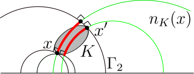
We consider in the upper half-plane model of . Let be a normal geodesic to . By applying an isometry, we may assume that is the -axis, so that the family of geodesics perpendicular to consists of concentric half circles (see Figure 7). By Santaló’s Lemma 3.10, only one line of (which we denote by ) intersects perpendicularly. Since has constant width, the projection of on the normal line has length .
Let be the points of intersection between and , and let , be the rays emanating from the base point of and passing through , respectively. Each such ray has the property of being equidistant to , i.e. it consists of points at some fixed distance from . Equivalently, they are orthogonal to every line of . Therefore every geodesic , intersects orthogonally at the points , and we have .
Since , the geodesics perpendicular to at do not intersect for , see Figure 7. Thus, the projection of on is strictly contained in the segment , and we have
∎
Remark 4.3.
In contrast to the maximal projection being obtained on a diameter (see Lemma 3.7), a minimal projection does not exist. Indeed, for any convex body , an arbitrarily small projection can be found. It can be shown that if a line intersects , and is a point sufficiently far from , then the projection of onto the line perpendicular to at can be made arbitrarily small. Thus the spectrum of projection lengths is the interval .
Theorem 4.4.
Let be a body of constant width , containing the origin in its interior, and such that is a -smooth curve. If all projection lengths of on are constant, then is a disc.
Proof.
By Lemma 3.8, the normal field of covers the interior of . Therefore there is a normal geodesic to which belongs to . On this geodesic, the width and the length of the projection coincide. Hence, all projections of on have length . By Proposition 4.2, this implies that each line in is a normal line, i.e., , which implies that is a disc.
∎
Corollary 4.5.
Let be a body of constant width , containing the origin in its interior, and such that is a -smooth curve. If all sections of on have constant length, then is a disc.
Proof.
The argument is very similar to the proof of Theorem 4.4. Since the normal field of covers the interior, there is a double normal geodesic that belongs to . By Lemma 3.5 and Proposition 4.2, the length of the section equals the width . Hence, all sections of on have length , and the conclusion follows again as in the proof of Theorem 4.4. ∎
Finally, to prove the characterization of the disc by properties and , we require the following lemma.
Lemma 4.6.
Let be a convex body with a -smooth boundary. Let be an equichordal point for . Then a normal geodesic line passing through must be a double normal.
Proof.
Let such that . For each , let be the geodesic passing through and , and let the other boundary point of belonging to . We consider a parametrization , of , such that , and with the property that if for , then .
We define the function to be the distance from the equichordal point to the corresponding boundary point of , i.e. . The equichordal hypothesis says that for some constant , any satisfies . Since the normal geodesic to at passes through , we have that . Then, for small ,
and
Adding the previous two equations we obtain that for every small enough
which implies that , thus is a double normal. ∎
Theorem 4.7.
Let be a convex body, containing the origin in its interior, such that is a -smooth curve. If every section of by a geodesic from has constant length , and every projection of on a geodesic in has constant length , then is a disc (and ).
Proof.
Let be the closest point in to the origin. Then the line containing the segment is a normal line of . By Lemma 4.6, is a double normal line, hence by Lemma 3.5. This implies . But then all projections and sections on have the same length, and therefore every geodesic in is a double normal geodesic of . Since is a curve orthogonal to all rays through the origin, is a disc. ∎

4.2. Orthogonal and non-orthogonal projections
As we have seen, the lengths of projections and the width are two distinct sources of information in the hyperbolic setting. Theorem 4.4 is based on using both to obtain a hyperbolic result which has no Euclidean analogue. Another example of this situation is given by orthogonal and non-orthogonal projections: In the Euclidean plane, knowing the length of an orthogonal projection of a convex body on a line gives us the same information as knowing the length of a non-orthogonal projection on a line forming a known angle with (see Figure 8). However, in the hyperbolic setting, knowing the lengths of orthogonal and non-orthogonal projections provides additional information that allows us to recover the body.
Let be a convex body and let be an interior point of . For each line we consider another line , chosen in the following way. We can assume that is a vertical line in the upper half-plane model. If are the two supporting geodesics of that are perpendicular to , we choose another vertical line at (Euclidean) distance from , such that intersects both supporting geodesics (see Figure 9). By compactness, the positive number can be chosen as the same for all lines .
Proposition 4.8.
Let be a convex body and let be an interior point of . Then is determined by the projection lengths
Proof.

For a given geodesic , we will call and . Let be the radius of and be the radius of (see Figure 9). Then
Therefore, and are determined from , and , and the intersection of all such strips between supporting geodesics uniquely determines the body. ∎
5. Appendix
We show that the hyperbolic Reuleaux triangle defined below has constant width and non constant sections and projections on . We work in the upper-plane model of . On the circle with hyperbolic center and hyperbolic radius 1, we choose three equidistant points, with one of them being (see Figure 10). For each of the three points, we trace the hyperbolic circle centered at that point and containing the other two. The resulting figure is the hyperbolic Reuleaux triangle, which has constant width since given one of the circular sides of the triangle, all of its normals pass through the opposite vertex of the triangle. The width can be computed by finding the distance between the intersection points of the Reuleaux triangle with the -axis, and its value is .

We show that there are two geodesics in on which the sections and projections of are different. First, on the vertical line passing through , the section and the projection of the Reuleaux triangle coincide, and their length is equal to the width of . Consider now the geodesic through forming a 90 degree angle with the vertical geodesic. We explicitly determine the points and where intersects the boundary of by solving the system formed by the equations of these two circles. The length of the section of by can then be exactly computed with Mathematica (though the expression is very long), and its approximate value is . Similarly, to compute the length of the projection of on this geodesic, we first find the geodesic , normal to , that is tangent to (the point of tangency is in Figure 10); next, we explicitly find the point of intersection of and , again by solving the system of the equations of the circles. The length of the projection of onto is approximately .
We observe that one can also construct a -smooth body of constant width which is a perturbation of a disc and does not have constant sections nor projections through .
References
- [1] Araújo P.V., Minimum Area of a Set of Constant Width in the Hyperbolic Plane. Geometriae Dedicata 64, issue 1, 41–53 (1997).
- [2] Berger M., Geometry. Springer Universitext (2009).
- [3] Dekster B.V., Double Normals Characterize Bodies of Constant Width in Riemannian Manifolds. Geometric Analysis and Nonlinear Partial Differential Equations, Lecture Notes in Pure and Applied Mathematics 144, 187–201, New York, (1993).
- [4] Gallego E., Reventós A., Solanes G., Teufel E., Width of Convex Bodies in Spaces of Constant Curvature, Manuscripta Mathematica 126, issue 1, 115–134 (2008).
- [5] Gardner R.J., Geometric Tomography. Cambridge University Press (1995).
- [6] Hiripitiyage K.L.H., Yaskin V., On Sections of Convex Bodies in Hyperbolic Space. Journal of Mathematical Analysis and Applications 445, 1394–1409 (2017).
- [7] Jerónimo-Castro J., Jimenez-Lopez F.G., A Characterization of the Hyperbolic Disc Among Constant Width Bodies. Bulletin of the Korean Mathematical Society 54, no. 6, 2053–2063 (2017).
- [8] Leichtweiss K., Curves of Constant Width in the Non-Euclidean Geometry. Abhandlungen aus dem Mathematischen Seminar der Universität Hamburg 75, issue 1, 257–284 (2005)
- [9] Ratcliffe J.G., Foundations of Hyperbolic Manifolds. Springer, New York, (1994).
- [10] Santaló L.A., Note on Convex Curves on the Hyperbolic Plane. Bulletin of the American Mathematical Society 51, 405–412 (1945).
- [11] Yaskin V., The Busemann-Petty Problem in Hyperbolic and Spherical Spaces. Advances in Mathematics 203, issue 2, 537–553 (2006).