Unsupervised Robust Disentangling of
Latent Characteristics for Image Synthesis

Let $x$ denote an image from an unknown data distribution $p_{\mathcal{X}}(x)$. Probabilistic approaches to image synthesis approximate the unknown distribution using a model distribution $p(x)$. To fit this distribution to the data distribution, the maximum log-likelihood of data samples is maximized:

$$\max_{p}\mathbb{E}_{x\sim p_{\mathcal{X}}(x)}\log p(x)$$

(1)

The distribution $p$ can then be sampled to synthesize new images. To model $p$, latent variable models assume that images are generated due to an underlying latent variable $z$ which is not observed. The full model distribution

$$p(x,z)=p(x|z)p(z)$$

(2)

is then specified in terms of the factors $p(x|z)$, which are typically parameterized by a function class such as neural networks, and the factor $p(z)$ which specifies a prior on the latent variable, typically given by a simple distribution like a normal distribution.

A Generative Adversarial Network (GAN) [15] learns such a model using density ratio estimation. The training algorithm can be described as a two player game: A classifier tries to distinguish between generated and real images; a generator tries to generate images that are indistinguishable from real images. Because no inference process is learned, they cannot explain existing images.

The Variational Autoencoder (VAE) [29, 48] learns a latent variable model using variational inference and the reparameterization trick. The structure of the joint $p(x,z)$ and the corresponding encoder distribution $q(z|x)$ is shown in Fig. 3a. Variational inference involves a KL regularization of $q(z|x)$ towards the prior $p(z)$ and VAEs choose $q$ such that it can be computed efficiently, e.g. Gaussian parameterizations [29, 48] or normalizing flows [28]. To increase the flexibility of encoder distributions, [44] uses an adversarial approach that requires only samples to compute the KL regularization. Similar to GANs, it involves a two player game. This time, a classifier has to distinguish between latent codes sampled from the prior and those sampled from the encoder distribution, and the second player is the encoder.

However, images are the product of two independent factors, pose $\pi$ and appearance $\alpha$. There are both variational [21] and adversarial approaches [22] that try to discover such disentangled factors without any additional source of information. But simply assuming that $\pi$ and $\alpha$ are different components of $z$, i.e. $z=(\pi,\alpha)$ is problematic because the prior $p(z)$ cannot model the individual contribution of pose and appearance without inductive biases [39, 55]. The resulting models fall short in comparison to approaches that can leverage additional information [17, 30]. Thus, to learn a model in which the generative process is described by $p(x|\pi,\alpha)$ we need additional information.

The common assumption of many recent works on disentangled image generation, e.g., [41, 42, 13, 2, 54, 12], is the observability of $\pi$, which is derived from a pretrained model for keypoint detection. While this representation of $\pi$ works quite well, it is limited to domains where robust keypoint detectors are available and sidesteps the learning task of disentangling the two latent factors $\pi,\alpha$. Instead, let us assume for a moment that we can observe samples of image triplets $(x_{1},x_{2},x_{3})$ with the constraints that (i) $x_{1}$, $x_{2}$ have the same appearance, (ii) $x_{2}$, $x_{3}$ share the same pose, and (iii) $x_{1}$, $x_{3}$ have neither pose nor shape in common. Let $p_{\mathbb{T}}(x_{1},x_{2},x_{3})$ denote this unknown joint distribution. We model each of the three images as being generated by a process of the form $p(x|\pi,\alpha)$ (which is assumed to be the same for all three images). Because $x_{1},x_{2}$ share appearance and $x_{2},x_{3}$ share pose, only four instead of six latent variables are required to explain how these triplets are generated. Let $\pi,\alpha$ denote the shared pose and appearance explaining $x_{2}$ and let $\pi^{\prime},\alpha^{\prime}$ denote additional realizations of pose and appearance explaining $x_{1}$ and $x_{3}$, respectively. The marginal distributions underlying $\pi$ and $\pi^{\prime}$ are assumed to be the same and so are the marginal distributions of $\alpha$ and $\alpha^{\prime}$. If, as assumed in [46, 32], we could observe the complete triplet $(x_{1},x_{2},x_{3})$, a simple inference mechanism would infer $\alpha$ from $x_{1}$ and $\pi$ from $x_{3}$ as depicted in Fig. 3b. Unfortunately, the assumption that $x_{2},x_{3}$ share the same pose but not appearance is essentially equivalent to the assumption that a keypoint estimator is implicitly available. Then pairs $x_{2},x_{3}$ could be found by comparison of keypoints. Without this information we have to further reduce assumptions on the data and essentially train without $x_{3}$.

Without access to $x_{3}$, we must rely on $x_{2}$ to infer $\pi$ as shown in Fig. 3c. The maximum likelihood objective for $p(x_{2}|\pi,\alpha)$ leads to a reconstruction loss, and without constraints on $\pi$ it encourages a degenerate solution where all information about $x_{2}$ is encoded in $\pi$ [43, 17], i.e. $\pi$ also encodes information about $\alpha$ instead of being independent of it.

[27] assumes the availability of labels for $\alpha$ and uses a conditional variant of the VAE, which results in a KL regularization of $q(\pi|x_{2})$ towards a prior and thus a constraint on $\pi$. To improve image generations with swapped $\alpha$ and $\pi$, [43] adds an adversarial constraint on generated images. It encourages the preservation of characteristics of $\alpha$, i.e. it combines the conditional VAE with a conditional GAN similar to [3]. [55] also utilize this GAN constraint but they only require pairs $x_{1},x_{2}$ instead of labels for $\alpha$, and instead of using the KL term to constrain $\pi$, they severely reduce its dimensionality. As pointed out by [17], these GAN constraints only encourage the decoder to ignore information about $\alpha$ in $\pi$ instead of disentangling $\alpha$ and $\pi$. [17] proposes a cycle-consistent VAE which adds a cyclic loss to the VAE objective. [40] directly models $\pi$ as keypoints. All of these methods rely on the same basic principle for disentanglement: Constraining the amount of information in $\pi$. Indeed, the VAE objective implements a variational approximation of the information bottleneck [1]. In contrast, we utilize this variational information bottleneck only to counteract overpowering, an issue that affects the following methods.

Similar to [44] for variational inference, [10] utilizes an adversarial approach for disentanglement: A classifier has to predict if a pair $(\pi,\pi^{\prime})$ was inferred from two images of the same video sequence or different video sequences. [16] assumes that $\alpha$ is given in the form of class labels, and [33, 19] are specialized to images of faces and assume that $\alpha$ is given in the form of facial attributes but they utilize the same principle: A classifier has to predict $\alpha$ from $\pi$. Besides differences in the precise objectives used for the classifiers, all of these methods implement again an information bottleneck as in [4]. Compared to variational approximations of the bottleneck, they have the advantage that only information about $\alpha$ in $\pi$ is penalized. However, applications of adversarial approaches have been limited to synthetic datasets or facial datasets with little to no pose variations. We show that overpowering prevents their direct application to real world datasets and show how to turn them into robust methods for disentanglement. Our approach can recombine pose and appearance of any two images, while previous models for unsupervised image-to-image translation require seperate training for each appearance [24, 35] and cannot transfer to unseen appearances [8].

We want to learn a probabilistic model of images that explains the observed image $x_{2}$ in terms of two disentangled representations $\pi,\alpha$. This requires a model for the decoder distribution conditioned on the two representations,

$$p(x_{2}|\pi,\alpha)$$

(3)

and an encoder model $p(\pi,\alpha|x_{1},x_{2})$ to infer $\pi$ and $\alpha$ from the data. As shown in Fig. 3c, we estimate $\pi$ with an encoder network $E_{\pi}(x_{2})$ from $x_{2}$ and $\alpha$ with an encoder network $E_{\alpha}(x_{1})$ from $x_{1}$. A decoder network $D(\pi,\alpha)$ which takes $\pi$ and $\alpha$ as inputs reconstructs the image according to $p(x_{2}|\pi,\alpha)$.

Learning the weights of these networks depends on a constrained optimization problem. To ensure that $\pi$ and $\alpha$ describe the images well, we maximize the conditional likelihood as formulated in Eq. (4), which corresponds to a reconstruction loss. To avoid a trivial solution where $\pi$ encodes all of the information of $x_{2}$, we formulate the disentanglement constraint (5), such that our full optimization problem reads

		$\displaystyle\max_{p}\mathbb{E}_{x_{1},x_{2}}\log p(x_{2}|\pi,\alpha)$		(4)
		$\displaystyle\text{subject to }I(\pi,\alpha)\leq\epsilon$		(5)

Here, $\epsilon$ is a small constant and $I(\pi,\alpha)$ denotes the mutual information [9] defined as

$$I(\pi,\alpha)=\KL(p(\pi,\alpha)|p(\pi)p(\alpha)).$$

(6)

Computing (6) is difficult [4] and to derive an algorithm for the solution of the optimization problem above, we must resort to approximations. Subsequently, we first derive two different estimates on the mutual information. The first one provides an upper bound, but, alas, it always overestimates it severely. A second estimate is then introduced which provides accurate estimates. However, to enforce the constraint in (5), we require gradients of the estimate and, as we will see, this enables the encoder to perform an adversarial attack on the estimate, such that it heavily underestimates the true mutual information. In Sec. 3.4, we show how to combine both estimates to obtain our method for robust maximum-likelihood learning under mutual information constraints. Thereafter, we describe the algorithm used to implement the method.

Ideally, we would like to obtain an upper bound on the MI in (6) to be able to enforce the constraint (5). Because we estimate $\pi$ from $x_{2}$ and $\alpha$ from $x_{1}$, we have the Markov-Chain $\pi\to x_{2}\to\alpha$ with

$$p(\alpha,x_{2},\pi)=p(\alpha|x_{2})p(x_{2}|\pi)p(\pi)$$

(7)

which implies the data processing inequality [9]:

$$I(\pi,\alpha)\leq I(\pi,x_{2}).$$

(8)

The right hand side of this inequality can now be easily estimated with a variational marginal $r(\pi)$ [1]. Indeed, for any density $r$ with respect to $\pi$ we have the bound

$$I(\pi,\alpha)\leq\mathbb{E}_{x_{2}}\KL(p(\pi|x_{2})|r(\pi)).$$

(9)

Modeling both $p(\pi|x_{2})$ and $r(\pi)$ as Gaussian distributions, we can evaluate the right hand side analytically. Unfortunately, this bound is too loose for our purposes. The condition $\KL(p(\pi|x_{2})|r(\pi))=0$ implies $I(\pi,x_{2})=0$ and thus $\pi$ would be completely uninformative.

A different estimate of mutual information can be obtained with the help of density estimation [44, 4]. The KL-divergence of two densities is closely related to the associated classification problem: Let $T(\pi,\alpha)$ be a classifier that maps a pair $(\pi,\alpha)$ to a real number which represents the log probability that the pair is a sample from the joint distribution $p(\pi,\alpha)$. Denote by $\sigma(t)=(1+e^{-t})^{-1}$ the sigmoid function. The maximum likelihood objective for this classification task reads

	$\displaystyle\max_{T}\;$	$\displaystyle\mathbb{E}_{(\pi,\alpha)\sim p(\pi,\alpha)}\log\sigma(T(\pi,\alpha))+$		(10)
		$\displaystyle\mathbb{E}_{\pi\sim p(\pi),\alpha\sim p(\alpha)}\log(1-\sigma(T(\pi,\alpha))).$		(11)

The optimal solution $T^{*}$ of this problem satisfies

$$I(\pi,\alpha)=\mathbb{E}_{(\pi,\alpha)\sim p(\pi,\alpha)}T^{*}(\pi,\alpha).$$

(12)

When $T$ is implemented as a neural network, we obtain a differentiable estimate of $I(\pi,\alpha)$ which can be used to enforce the desired constraint during learning of $q(\pi|x_{2})$. For a given classifier $T$ we write $I_{T}=I_{T}(\pi,\alpha)=\mathbb{E}_{\pi,\alpha\sim p(\pi,\alpha)}T(\pi,\alpha)$ for the resulting estimate.

If we replace the constraint $I(\pi,\alpha)\leq\epsilon$ in (5) with a constraint on the estimate $I_{T}(\pi,\alpha)\leq\epsilon$, we observe a new type of adversarial attack: The encoder is able to overpower the classifier $T$: it can learn a distribution $p(\pi|\alpha)$ such that $T$ cannot differentiate pairs $(\pi,\alpha)$ sampled from the joint from those sampled from the marginals. However, a seperately trained classifier $T^{\prime}$, whose gradients are not provided to the encoder, can still classify them (see Fig. 1). In other words, in an adversarial setting we consistently observe the situation $I_{T}(\pi,\alpha)\ll I(\pi,\alpha)$, i.e., we underestimate the mutual information between $\pi$ and $\alpha$. To obtain a guaranteed upper bound on the mutual information, we must utilize the variational upper bound. As we have seen before, we must be careful to enforce not too strict bounds on it. Thus, we formulate our new objective as

		$\displaystyle\max_{p}\mathbb{E}_{x_{1},x_{2}}\log p(x_{2}|\pi,\alpha)$		(13)
		$\displaystyle\text{subject to }I_{T}(\pi,\alpha)\leq\epsilon$		(14)
		$\displaystyle\phantom{subjectto}\KL(p(\pi|x_{2})|r(\pi))\leq C,$		(15)

where $C$ has to be adaptively estimated based on the detection of adversarial attacks of the encoder against $T$. The main idea is to compare the classification performance of $T$ against an independently trained classifier. If there is a large performance gap, we cannot rely on the estimate of $T$ (it has been overpowered) and must decrease $C$. The next section describes the approach.

To obtain a training signal for our networks, we must transform problem (13) into an unconstrained problem which can be optimized by gradient ascent. Let us first consider the constraint (15) on the $\KL$ term. For a given $C$, there exists a Lagrange multiplier $\gamma\geq 0$ such that the problem can be written equivalently as

		$\displaystyle\max_{p}\mathbb{E}_{x_{1},x_{2}}\log p(x_{2}|\pi,\alpha)-\gamma\KL(p(\pi|x_{2})|r(\pi))$		(16)
		$\displaystyle\text{subject to }I_{T}(\pi,\alpha)\leq\epsilon.$		(17)

Thus, we can directly estimate $\gamma$ instead of $C$. Ideally, $\gamma$ should be very small and only active in situations were $I_{T}(\pi,\alpha)$ underestimates the mutual information. To achieve this, we train a second classifier $T^{\prime}$ based on the same objective (10). It is crucial that its estimate $I_{T^{\prime}}(\pi,\alpha)$ is never directly provided as a signal to the encoder. We merely compare the estimates of $T$ and $T^{\prime}$ and if $I_{T}\ll I_{T^{\prime}}$, we increase $\gamma$. Hence, we update $\gamma$ in each optimization step based on the proportional gain $I_{T^{\prime}}-I_{T}$ and bias it towards zero with a small constant $b_{\gamma}$

$$\gamma_{t+1}=\max\{0,\gamma_{t}+l_{\gamma}(I_{T^{\prime}}-I_{T}-b_{\gamma})\},$$

(18)

where $l_{\gamma}$ can be considered the learning rate of $\gamma$.

For the remaining constraint (17) on $I_{T}(\pi,\alpha)$, we utilize an Augmented Lagrangian Approach [60]. After switching from maximization to minimization, the complete unconstrained loss function $\mathcal{L}$ for training the network is

$$\mathcal{L}=\mathcal{L}_{\text{rec}}+\mathcal{L}_{\text{VB}}+\mathcal{L}_{\text{MI}},$$

(19)

where $\mathcal{L}_{\text{rec}}$ is the reconstruction loss given by the negative likelihood

$$\mathcal{L}_{\text{rec}}=-\mathbb{E}_{x_{1},x_{2}}\log p(x_{2}|\pi,\alpha),$$

(20)

$\mathcal{L}_{\text{VB}}$ the penalty associated with the variational upper bound

$$\mathcal{L}_{\text{VB}}=\gamma\KL(p(\pi|x_{2})|r(\pi)),$$

(21)

and $\mathcal{L}_{\text{MI}}$ the loss used to enforce the the constraint (17) based on an estimated Lagrange multiplier $\lambda\geq 0$ and a penalty parameter $\mu>0$

$$\mathcal{L}_{\text{MI}}=\begin{cases}\lambda(I_{T}-\epsilon)+\frac{\mu}{2}(I_{T}-\epsilon)^{2}\quad&\text{if }I_{T}-\epsilon\geq-\frac{\lambda}{\mu}\\ -\frac{\lambda^{2}}{2\mu}\quad&\text{else}\end{cases}.$$

(22)

The update rule for $\lambda$ is

$$\lambda_{t+1}=\max\{0,\lambda_{t}+\mu(I_{T}-\epsilon)\}.$$

(23)

Fig. 4 outlines our network architecture during training and inference. We perform the optimization over mini-batches and alternate between the training of the classifiers $T$ and $T^{\prime}$ (according to the objective defined in (10)), and the training of the generative model. The loss for the networks $D$ and $E_{\alpha}$ is given by $\mathcal{L}_{\text{rec}}$ and $E_{\pi}$ is optimized with respect to the full loss $\mathcal{L}$. After each step, $\gamma$ and $\lambda$ are updated according to (18) and (23), respectively.

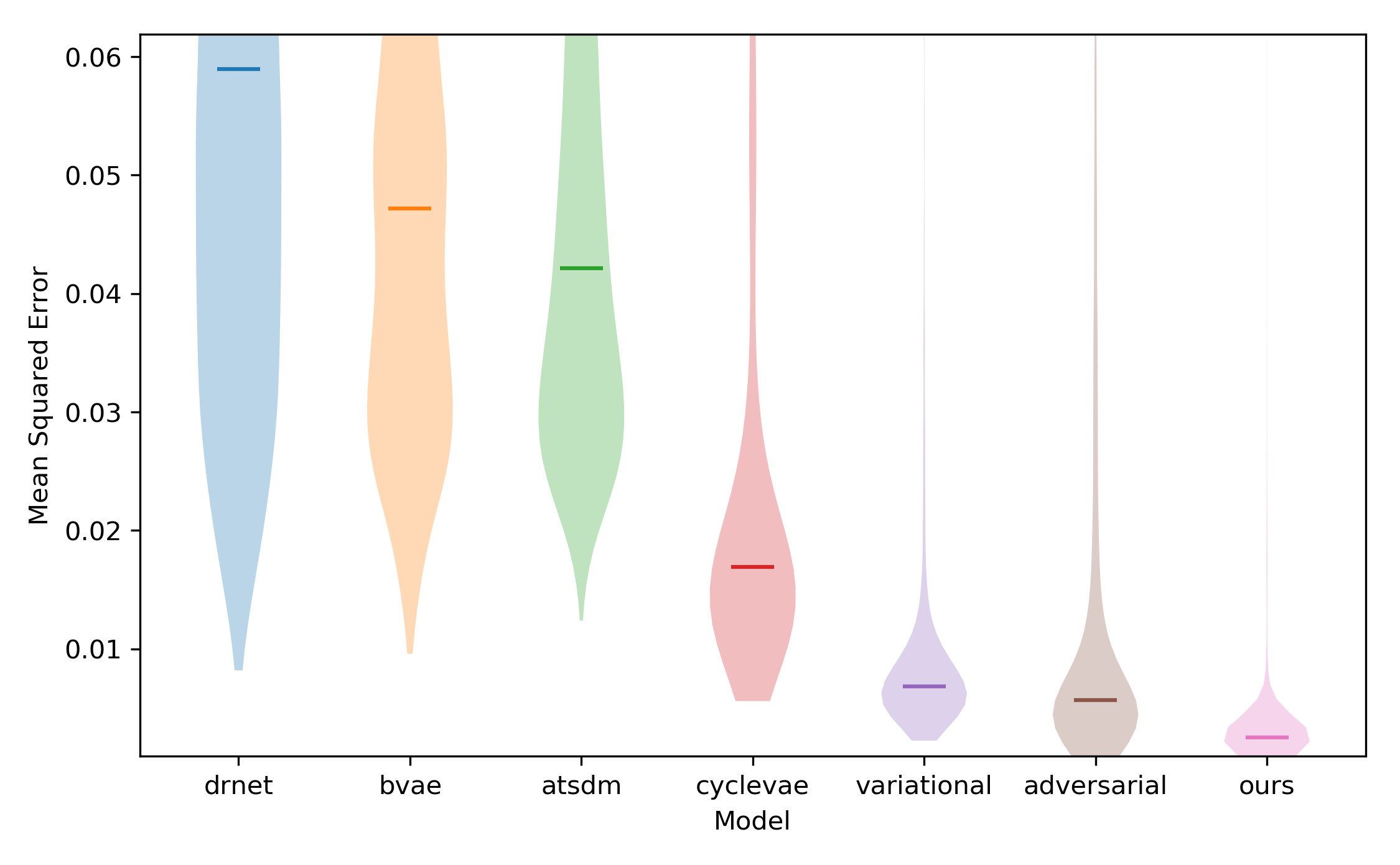
In Fig. 7, we compare our method to [17] (cyclevae), the state-of-the-art among the variational approaches, and to [16] (atsdm), the state-of-the-art among the adversarial approaches. In addition to our full model (ours), we also include [10] (drnet), a version of our model that utilizes the objective of [21] (bvae), a version without $\mathcal{L}_{\text{VB}}$ (adversarial) and a version without $\mathcal{L}_{\text{MI}}$ (variational), where the update of $\gamma$ from (18) is replaced by

$$\gamma_{t+1}=\max\{0,\gamma_{t}+l_{\gamma}(I_{T^{\prime}}-\epsilon)\},$$

(24)

to estimate the required $\gamma$ to achieve the MI constraint (5).

Because it is difficult to obtain ground truth for triplets $(x_{1},x_{2},x_{3})$ on real data, we resort to the synthetic sprites dataset [46] to compare the methods. It contains 672 different video game characters, each depicted in a wide variety of poses. For training, we only utilize pairs of images $(x_{1},x_{2})$ belonging to the same character. To measure the performance of the different approaches, we calculate the mean squared error between images $\tilde{x}_{2}$ generated from inputs $x_{1}$ and $x_{3}$, and the corresponding ground truth $x_{2}$. We randomly select 8000 triplets $(x_{1},x_{2},x_{3})$ from the test set and report the error distribution in Fig. 7.

To better understand the information encoded by $\pi$ and $\alpha$, we visualize these representations. Because $\pi$ does not contain information about the appearance, this corresponds to a marginalization of images depicting a given pose over all appearances. Similarly, $\alpha$ yields a marginalization for a given appearance over all poses. We show examples of these visualizations in Fig. 1, Tab. 1, and Fig. 5. This synthesis is performed independently from the training of our model with the sole purpose of interpretability and visualization. For this, a decoder network is trained to reconstruct images from only one of the factors. In Tab. 1, these visualizations demonstrate that $I_{T^{\prime}}$ estimates entanglement correctly. In that figure, a) is our model without $\mathcal{L}_{\text{MI}}$ and the update of $\gamma$ replaced by (24). b) is our model without $\mathcal{L}_{\text{VB}}$, c) with $b_{\gamma}=0$, d) with $\gamma=1$ fixed and e) is our full model.

The previous dataset contained a single category of objects, namely video game characters. In this setting, a common pose representation is relatively easily defined in terms of a skeleton. It is considerably more difficult to find a representation of pose that works across different object categories which do not share a common shape. To evaluate our model in this situation, we utilize the NORB dataset [34], which contains images of 50 toys belonging to 5 different object categories. Each instance is depicted under a wide variety of camera views and lighting conditions. For this experiment, we consider camera views and lighting conditions to be represented by $\pi$. In Fig. 5 we can see that our model successfully finds two representations that can be combined across different object categories. Note that our model was never trained on a pair of images depicting instances of different categories.

In Tab. 2, we evaluate our approach on natural images of people, which have been the subject of recent models for disentangled image generation [13]. Besides qualitative evaluations, we employ two quantitative measures to validate how much of the pose and appearance are being preserved in the generated output: (i) Since ground-truth triplets are not available for these datasets, we require a metric that captures similarity in appearance while being invariant to changes in pose. Such a measure can be obtained from a person reidentification model [20], which can identify the same person despite differences in pose. Using the evaluation protocol of [20] we report the mean average precision (mAP) of re-identifying generated images under “reID mAP” in Tab. 2. (ii) To measure how well our approach retains pose we employ Openpose [5] to obtain keypoint estimates. We extract keypoints from the pose input image $x_{3}$ and the output $x_{2}$ and compute the euclidean distance between the estimated keypoints in both images. As above, we include an ablation (adversarial) without $\mathcal{L}_{\text{VB}}$.

References

- [1] Alexander A Alemi, Ian Fischer, Joshua V Dillon, and Kevin Murphy. Deep variational information bottleneck. arXiv preprint arXiv:1612.00410, 2016.
- [2] Guha Balakrishnan, Amy Zhao, Adrian V Dalca, Fredo Durand, and John Guttag. Synthesizing images of humans in unseen poses. In Proceedings of the IEEE Conference on Computer Vision and Pattern Recognition, pages 8340–8348, 2018.
- [3] Jianmin Bao, Dong Chen, Fang Wen, Houqiang Li, and Gang Hua. Cvae-gan: fine-grained image generation through asymmetric training. In Proceedings of the IEEE International Conference on Computer Vision, pages 2745–2754, 2017.
- [4] Ishmael Belghazi, Sai Rajeswar, Aristide Baratin, R Devon Hjelm, and Aaron Courville. Mine: mutual information neural estimation. arXiv preprint arXiv:1801.04062, 2018.
- [5] Zhe Cao, Tomas Simon, Shih-En Wei, and Yaser Sheikh. Realtime multi-person 2d pose estimation using part affinity fields. In CVPR, 2017.
- [6] James Charles, Tomas Pfister, Mark Everingham, and Andrew Zisserman. Automatic and efficient human pose estimation for sign language videos. International Journal of Computer Vision, 110(1):70–90, 2014.
- [7] Xi Chen, Yan Duan, Rein Houthooft, John Schulman, Ilya Sutskever, and Pieter Abbeel. Infogan: Interpretable representation learning by information maximizing generative adversarial nets. In Advances in Neural Information Processing Systems, pages 2172–2180, 2016.
- [8] Yunjey Choi, Minje Choi, Munyoung Kim, Jung-Woo Ha, Sunghun Kim, and Jaegul Choo. Stargan: Unified generative adversarial networks for multi-domain image-to-image translation. In Proceedings of the IEEE Conference on Computer Vision and Pattern Recognition, pages 8789–8797, 2018.
- [9] Thomas M Cover and Joy A Thomas. Elements of information theory. John Wiley & Sons, 2012.
- [10] Emily L Denton and Vighnesh Birodkar. Unsupervised learning of disentangled representations from video. In I. Guyon, U. V. Luxburg, S. Bengio, H. Wallach, R. Fergus, S. Vishwanathan, and R. Garnett, editors, Advances in Neural Information Processing Systems 30, pages 4414–4423. Curran Associates, Inc., 2017.
- [11] Alexey Dosovitskiy and Thomas Brox. Generating images with perceptual similarity metrics based on deep networks. In Advances in Neural Information Processing Systems, pages 658–666, 2016.
- [12] Patrick Esser, Johannes Haux, Timo Milbich, et al. Towards learning a realistic rendering of human behavior. In Proceedings of the European Conference on Computer Vision (ECCV), pages 0–0, 2018.
- [13] Patrick Esser, Ekaterina Sutter, and Björn Ommer. A variational u-net for conditional appearance and shape generation. In Proceedings of the IEEE Conference on Computer Vision and Pattern Recognition, pages 8857–8866, 2018.
- [14] Heng Fan, Liting Lin, Fan Yang, Peng Chu, Ge Deng, Sijia Yu, Hexin Bai, Yong Xu, Chunyuan Liao, and Haibin Ling. Lasot: A high-quality benchmark for large-scale single object tracking. arXiv preprint arXiv:1809.07845, 2018.
- [15] Ian Goodfellow, Jean Pouget-Abadie, Mehdi Mirza, Bing Xu, David Warde-Farley, Sherjil Ozair, Aaron Courville, and Yoshua Bengio. Generative adversarial nets. In Advances in neural information processing systems, pages 2672–2680, 2014.
- [16] Naama Hadad. A two-step disentanglement method. 2018 IEEE/CVF Conference on Computer Vision and Pattern Recognition, pages 772–780, 2018.
- [17] Ananya Harsh Jha, Saket Anand, Maneesh Singh, and VSR Veeravasarapu. Disentangling factors of variation with cycle-consistent variational auto-encoders. In Proceedings of the European Conference on Computer Vision (ECCV), pages 805–820, 2018.
- [18] Kaiming He, Xiangyu Zhang, Shaoqing Ren, and Jian Sun. Deep residual learning for image recognition. In Proceedings of the IEEE conference on computer vision and pattern recognition, pages 770–778, 2016.
- [19] Zhenliang He, Wangmeng Zuo, Meina Kan, Shiguang Shan, and Xilin Chen. Attgan: Facial attribute editing by only changing what you want. IEEE Transactions on Image Processing, 2019.
- [20] Alexander Hermans*, Lucas Beyer*, and Bastian Leibe. In Defense of the Triplet Loss for Person Re-Identification. arXiv preprint arXiv:1703.07737, 2017.
- [21] Irina Higgins, Loic Matthey, Arka Pal, Christopher Burgess, Xavier Glorot, Matthew Botvinick, Shakir Mohamed, and Alexander Lerchner. beta-vae: Learning basic visual concepts with a constrained variational framework. ICLR, 2(5):6, 2017.
- [22] Qiyang Hu, Attila Szabó, Tiziano Portenier, Paolo Favaro, and Matthias Zwicker. Disentangling factors of variation by mixing them. In Proceedings of the IEEE Conference on Computer Vision and Pattern Recognition, pages 3399–3407, 2018.
- [23] Lianghua Huang, Xin Zhao, and Kaiqi Huang. Got-10k: A large high-diversity benchmark for generic object tracking in the wild. arXiv preprint arXiv:1810.11981, 2018.
- [24] Xun Huang, Ming-Yu Liu, Serge Belongie, and Jan Kautz. Multimodal unsupervised image-to-image translation. In Proceedings of the European Conference on Computer Vision (ECCV), pages 172–189, 2018.
- [25] Justin Johnson, Alexandre Alahi, and Li Fei-Fei. Perceptual losses for real-time style transfer and super-resolution. In European Conference on Computer Vision, pages 694–711. Springer, 2016.
- [26] Diederik P Kingma and Jimmy Ba. Adam: A method for stochastic optimization. arXiv preprint arXiv:1412.6980, 2014.
- [27] Durk P Kingma, Shakir Mohamed, Danilo Jimenez Rezende, and Max Welling. Semi-supervised learning with deep generative models. In Advances in neural information processing systems, pages 3581–3589, 2014.
- [28] Durk P Kingma, Tim Salimans, Rafal Jozefowicz, Xi Chen, Ilya Sutskever, and Max Welling. Improved variational inference with inverse autoregressive flow. In Advances in neural information processing systems, pages 4743–4751, 2016.
- [29] Diederik P Kingma and Max Welling. Auto-encoding variational bayes. arXiv preprint arXiv:1312.6114, 2013.
- [30] Dmytro Kotovenko, Artsiom Sanakoyeu, Sabine Lang, and Björn Ommer. Content and style disentanglement for artistic style transfer. In Proceedings of the Intl. Conf. on Computer Vision (ICCV), 2019.
- [31] Alex Krizhevsky, Ilya Sutskever, and Geoffrey E Hinton. Imagenet classification with deep convolutional neural networks. In F. Pereira, C. J. C. Burges, L. Bottou, and K. Q. Weinberger, editors, Advances in Neural Information Processing Systems 25, pages 1097–1105. Curran Associates, Inc., 2012.
- [32] Tejas D Kulkarni, William F Whitney, Pushmeet Kohli, and Josh Tenenbaum. Deep convolutional inverse graphics network. In Advances in neural information processing systems, pages 2539–2547, 2015.
- [33] Guillaume Lample, Neil Zeghidour, Nicolas Usunier, Antoine Bordes, Ludovic DENOYER, and Marc Aurelio Ranzato. Fader networks:manipulating images by sliding attributes. In I. Guyon, U. V. Luxburg, S. Bengio, H. Wallach, R. Fergus, S. Vishwanathan, and R. Garnett, editors, Advances in Neural Information Processing Systems 30, pages 5967–5976. Curran Associates, Inc., 2017.
- [34] Yann LeCun, Fu Jie Huang, and Leon Bottou. Learning methods for generic object recognition with invariance to pose and lighting. In Computer Vision and Pattern Recognition, 2004. CVPR 2004. Proceedings of the 2004 IEEE Computer Society Conference on, volume 2, pages II–104. IEEE, 2004.
- [35] Hsin-Ying Lee, Hung-Yu Tseng, Jia-Bin Huang, Maneesh Singh, and Ming-Hsuan Yang. Diverse image-to-image translation via disentangled representations. In Proceedings of the European Conference on Computer Vision (ECCV), pages 35–51, 2018.
- [36] Hongye Liu, Yonghong Tian, Yaowei Wang, Lu Pang, and Tiejun Huang. Deep relative distance learning: Tell the difference between similar vehicles. In Proceedings of the IEEE Conference on Computer Vision and Pattern Recognition, pages 2167–2175, 2016.
- [37] Ziwei Liu, Ping Luo, Shi Qiu, Xiaogang Wang, and Xiaoou Tang. Deepfashion: Powering robust clothes recognition and retrieval with rich annotations. In Proceedings of IEEE Conference on Computer Vision and Pattern Recognition (CVPR), June 2016.
- [38] Ziwei Liu, Sijie Yan, Ping Luo, Xiaogang Wang, and Xiaoou Tang. Fashion landmark detection in the wild. In European Conference on Computer Vision (ECCV), October 2016.
- [39] Francesco Locatello, Stefan Bauer, Mario Lucic, Gunnar Raetsch, Sylvain Gelly, Bernhard Schölkopf, and Olivier Bachem. Challenging common assumptions in the unsupervised learning of disentangled representations. In International Conference on Machine Learning, pages 4114–4124, 2019.
- [40] Dominik Lorenz, Leonard Bereska, Timo Milbich, and Björn Ommer. Unsupervised part-based disentangling of object shape and appearance. In Proceedings of the IEEE Conference on Computer Vision and Pattern Recognition (CVPR), 2019.
- [41] Liqian Ma, Xu Jia, Qianru Sun, Bernt Schiele, Tinne Tuytelaars, and Luc Van Gool. Pose guided person image generation. In Advances in Neural Information Processing Systems, pages 405–415, 2017.
- [42] Liqian Ma, Qianru Sun, Stamatios Georgoulis, Luc Van Gool, Bernt Schiele, and Mario Fritz. Disentangled person image generation. In Proceedings of the IEEE Conference on Computer Vision and Pattern Recognition, pages 99–108, 2018.
- [43] Michael F Mathieu, Junbo Jake Zhao, Junbo Zhao, Aditya Ramesh, Pablo Sprechmann, and Yann LeCun. Disentangling factors of variation in deep representation using adversarial training. In Advances in Neural Information Processing Systems, pages 5040–5048, 2016.
- [44] Lars Mescheder, Sebastian Nowozin, and Andreas Geiger. Adversarial variational bayes: Unifying variational autoencoders and generative adversarial networks. In Proceedings of the 34th International Conference on Machine Learning-Volume 70, pages 2391–2400. JMLR. org, 2017.
- [45] Chris Olah, Alexander Mordvintsev, and Ludwig Schubert. Feature visualization. Distill, 2017. https://distill.pub/2017/feature-visualization.
- [46] Scott E Reed, Yi Zhang, Yuting Zhang, and Honglak Lee. Deep visual analogy-making. In C. Cortes, N. D. Lawrence, D. D. Lee, M. Sugiyama, and R. Garnett, editors, Advances in Neural Information Processing Systems 28, pages 1252–1260. Curran Associates, Inc., 2015.
- [47] Shaoqing Ren, Kaiming He, Ross Girshick, and Jian Sun. Faster r-cnn: Towards real-time object detection with region proposal networks. In Advances in neural information processing systems, pages 91–99, 2015.
- [48] Danilo Jimenez Rezende, Shakir Mohamed, and Daan Wierstra. Stochastic backpropagation and approximate inference in deep generative models. In Proceedings of the 31st International Conference on International Conference on Machine Learning-Volume 32, pages II–1278. JMLR. org, 2014.
- [49] Olaf Ronneberger, Philipp Fischer, and Thomas Brox. U-net: Convolutional networks for biomedical image segmentation. In International Conference on Medical image computing and computer-assisted intervention, pages 234–241. Springer, 2015.
- [50] Amir Shahroudy, Jun Liu, Tian-Tsong Ng, and Gang Wang. Ntu rgb+d: A large scale dataset for 3d human activity analysis. In The IEEE Conference on Computer Vision and Pattern Recognition (CVPR), June 2016.
- [51] Wenzhe Shi, Jose Caballero, Ferenc Huszár, Johannes Totz, Andrew P Aitken, Rob Bishop, Daniel Rueckert, and Zehan Wang. Real-time single image and video super-resolution using an efficient sub-pixel convolutional neural network. In Proceedings of the IEEE Conference on Computer Vision and Pattern Recognition, pages 1874–1883, 2016.
- [52] Karen Simonyan and Andrew Zisserman. Very deep convolutional networks for large-scale image recognition. arXiv preprint arXiv:1409.1556, 2014.
- [53] K. Simonyan and A. Zisserman. Very Deep Convolutional Networks for Large-Scale Image Recognition. ArXiv e-prints, Sept. 2014.
- [54] Adrian Spurr, Jie Song, Seonwook Park, and Otmar Hilliges. Cross-modal deep variational hand pose estimation. In Proceedings of the IEEE Conference on Computer Vision and Pattern Recognition, pages 89–98, 2018.
- [55] Attila Szabó, Qiyang Hu, Tiziano Portenier, Matthias Zwicker, and Paolo Favaro. Challenges in disentangling independent factors of variation. arXiv preprint arXiv:1711.02245, 2017.
- [56] Christian Szegedy, Wojciech Zaremba, Ilya Sutskever, Joan Bruna, Dumitru Erhan, Ian Goodfellow, and Rob Fergus. Intriguing properties of neural networks. arXiv preprint arXiv:1312.6199, 2013.
- [57] Christian Szegedy, Wojciech Zaremba, Ilya Sutskever, Joan Bruna, Dumitru Erhan, Ian Goodfellow, and Rob Fergus. Intriguing properties of neural networks. arXiv preprint arXiv:1312.6199, 2013.
- [58] Paul Upchurch, Jacob Gardner, Kavita Bala, Robert Pless, Noah Snavely, and Kilian Weinberger. Deep feature interpolation for image content changes. In Proc. IEEE Conf. Computer Vision and Pattern Recognition, pages 6090–6099, 2016.
- [59] Aaron van den Oord, Nal Kalchbrenner, Lasse Espeholt, koray kavukcuoglu, Oriol Vinyals, and Alex Graves. Conditional image generation with pixelcnn decoders. In D. D. Lee, M. Sugiyama, U. V. Luxburg, I. Guyon, and R. Garnett, editors, Advances in Neural Information Processing Systems 29, pages 4790–4798. Curran Associates, Inc., 2016.
- [60] Stephen Wright and Jorge Nocedal. Numerical optimization. Springer Science, 35(67-68):7, 1999.
- [61] Matthew D Zeiler and Rob Fergus. Visualizing and understanding convolutional networks. In European conference on computer vision, pages 818–833. Springer, 2014.
- [62] Liang Zheng, Liyue Shen, Lu Tian, Shengjin Wang, Jingdong Wang, and Qi Tian. Scalable person re-identification: A benchmark. In Computer Vision, IEEE International Conference on, 2015.
Supplementary materials for
Robust Disentanglement on Real-World Datasets without
Pose-Annotations
We provide additional results obtained by our method in Sec. A and implementation details in Sec. B.
Appendix A Synthesis Results
A.1 Object Image Generation
A.2 Person Image Generation
In Tab. 3 we provide a qualitative comparison to [13] which highlights the benefits of not requiring keypoint estimates even for domains where keypoint estimators are available. Our approach does not suffer from pose estimation errors and, compared to keypoints, our pose representation is better disentangled from appearance.
We show additional results for Person Image Generation in Fig. 11, Fig. 15 and Fig. 16. Note that our method learns an appearance invariant representation of pose across a wide range of poses and viewpoints (Fig. 11). Fig. 15 shows that it can handle fine grained pose representations such as those required for hands. Fig. 16 demonstrates the applicability of our method for general human actions. Fig. 12 shows interpolation along appearance and pose axes.
A.3 Video Generation
Requiring no pose annotations but only multiple images depicting the same object, our method can be directly applied to video data without additional annotations. Thus, we are also able to perform unsupervised video-to-video translation. We provide examples for the norb dataset (norb.avi), the bbc dataset (bbc.avi) as well as the ntu dataset (ntu.avi).
Appendix B Implementation Details
In this section we provide additional details on the implementation of our method.
B.1 Network Parameters
We use the following notation to describe the network architectures:
- •
conv(n): a convolutional layer with -kernel and filters.
down(n): a convolutional layer with -kernel, filters and stride .
up(n): a convolutional layer with -kernel, filters, followed by a reshuffling of pixels to upsample the feature map by a factor of . Also known as subpixel convolution [51].
act: a ReLU activation.
res: a residual block [18]: The input feature map plus the ReLU activated input feature map followed by a convolutional layer with -kernel with as many filters as the input feature map has channels.
Depending on the dataset, the generated images have resolution (sprites dataset), (norb dataset) or (remaining datasets). Both encoders and have the same architecture:
Encoders at resolution : conv(16), res, down(32), res, down(64), res, down(128), res, down(256), res, res, res, res, res, act, conv(16).
Encoders at resolution : conv(32), res, down(64), res, down(128), res, down(128), res, down(256), res, down(256), res, res, res, res, res, act, conv(16).
Encoders at resolution : conv(32), res, down(64), res, down(128), res, down(128), res, down(256), res, down(256), res, down(256), res, res, res, res, res, act, conv(16).
The decoder receives both and . Each of them is processed seperately by four res blocks and the result is concatenated. Depending on the resolution, the remaining decoder architecture is described by:
Decoder at resolution : conv(256), res, up(128), res, up(64), res, up(32), res, up(16), res, conv(3) .
Decoder at resolution : conv(256), res, up(256), res, up(128), res, up(128), res, up(64), res, up(32), res, conv(3) .
Decoder at resolution : conv(256), res, up(256), res, up(256), res, up(128), res, up(128), res, up(64), res, up(32), res, conv(3) .
The classifiers and have the same architecture. Both receive and , and process them seperately with a conv(512) layer, followed by four res blocks. The result is activated and processed through a final conv(512) layer before the output is computed as the inner product of the two resulting feature maps.
B.2 Model Parameters
For all experiments, we use and . and are both modeled as Gaussian distributions of unit variance. The latter has a mean of zero and estimates the mean of the first. We use the reparameterization trick [29] to obtain low variance estimates of the gradient. Depending on the dataset, we implement the negative log-likelihood with a loss (sprites), a perceptual loss [25] (norb) or a perceptual loss together with a discriminator loss as in [11], weighted by (remaining datasets).
B.3 Optimization Parameters
We train our model over batches of size for steps. We use the Adam optimizer [26] with an initial learning rate of linearly decayed to zero. We set and . is calculated with an exponential moving average with decay parameter .