Machine learning and serving of discrete field theories — when artificial intelligence meets the discrete universe
Abstract
A method for machine learning and serving of discrete field theories in physics is developed. The learning algorithm trains a discrete field theory from a set of observational data on a spacetime lattice, and the serving algorithm uses the learned discrete field theory to predict new observations of the field for new boundary and initial conditions. The approach to learn discrete field theories overcomes the difficulties associated with learning continuous theories by artificial intelligence. The serving algorithm of discrete field theories belongs to the family of structure-preserving geometric algorithms, which have been proven to be superior to the conventional algorithms based on discretization of differential equations. The effectiveness of the method and algorithms developed is demonstrated using the examples of nonlinear oscillations and the Kepler problem. In particular, the learning algorithm learns a discrete field theory from a set of data of planetary orbits similar to what Kepler inherited from Tycho Brahe in 1601, and the serving algorithm correctly predicts other planetary orbits, including parabolic and hyperbolic escaping orbits, of the solar system without learning or knowing Newton’s laws of motion and universal gravitation. The proposed algorithms are also applicable when effects of special relativity and general relativity are important. The illustrated advantages of discrete field theories relative to continuous theories in terms of machine learning compatibility are consistent with Bostrom’s simulation hypothesis.
Keywords:
Machine learning, Discrete field theory, Discrete universe1 Introduction and statement of the problem
Data-driven methodology has attracted much attention recently in the physics community. This is not surprising since one of the fundamental objectives of physics is to deduce or discover the laws of physics from observational data. The rapid development of artificial intelligence technology begs the question of whether such deductions or discoveries can be carried out algorithmically by computers.
In this paper, I propose a method for machine learning of discrete field theories in physics from observational data. The method also includes an effective algorithm to serve the discrete field theories learned, in terms of predicting new observations.
Machine learning is not exactly a new concept in physics. In particular, the connection between artificial neural networks and dynamical systems has been noticed for decades (Narendra and Parthasarathy 1990; Narendra and Parthasarathy 1992; Ramacher 1993; Howse et al. 1995; Wilde 1993; E 2017; Chen et al. 2018; Haber and Ruthotto 2018). What is the new contribution brought by the present study? Most current applications of machine learning techniques in physics can be roughly divided into the following categories. (i) Using neural networks to model complex physical processes, such as plasma disruptions in magnetic fusion devices (Wroblewski et al. 1997; Vannucci et al. 1999; Yoshino 2003; Kates-Harbeck et al. 2019), effective Reynolds stress due to turbulence (Wu et al. 2018), coarse-grained nonlinear effects (Bar-Sinai et al. 2019), and proper moment closure schemes for fluid systems (Han et al. 2019). (ii) Solving differential equations in mathematical physics by approximating solutions with neural networks (Dissanayake and Phan-Thien 1994; Meade and Fernández 1994a; Meade and Fernández 1994b; Lagaris et al. 1998; Bailer-Jones et al. 1998; Long et al. 2019). In particular, significant progress has been made in solving Schrödinger’s equation for many-body systems (Carleo and Troyer 2017; Nomura et al. 2017). (iii) Discovering unknown functions or undetermined parameters in governing differential equations (Bongard and Lipson 2007; Schmidt and Lipson 2009; Brunton et al. 2016; Rudy et al. 2017; Schaeffer 2017; Baydin et al. 2017; Raissi 2018; Cranmer et al. 2019a; Gelß et al. 2019; Raissi et al. 2019). As a specific example, methods of learning the Hamiltonian function of a canonical symplectic Hamiltonian system were proposed in recent months (Wu et al. 2019; Lutter et al. 2019; Bertalan et al. 2019; Greydanus et al. 2019; Zhong et al. 2019; Sanchez-Gonzalez et al. 2019; Chen et al. 2019; Toth et al. 2019). (iv) Using neural networks to generate sampling data in statistical ensembles for calculating equilibrium properties of physical systems (Shanahan et al. 2018; Noé et al. 2019; Halverson et al. 2019; Cranmer et al. 2019b).
The problem addressed in this paper belongs to a new category. The method proposed learns a field theory from a given set of training data consisting of observed values of a physical field at discrete spacetime locations. The laws of physics are fundamentally expressed in the form of field theories instead of differential equations. It is thus more important to learn the underpinning field theories when possible. Since field theories are in general simpler than the corresponding differential equations, learning field theories is easier, which is true for both human intelligence and artificial intelligence. Except for the fundamental assumption that the observational data are governed by field theories, the learning and serving algorithms proposed do not assume any knowledge of the laws of physics, such as Newton’s law of motion and Schrödinger’s equation. This is a stark contrast to all other methodologies of machine learning in physics.
Without losing of generality, let’s briefly review the basics of field theories using the example of first-order field theory in the space of for a scalar field . A field theory is specified by a Lagrangian density where are the coordinates for . The theory requires that with the value of fixed at the boundary, varies with respect to in such a way that the action of the system
| (1) |
is minimized. Such a requirement of minimization is equivalent to the condition that the following Euler-Lagrange (EL) equation is satisfied everywhere in ,
| (2) |
The problem of machine learning of field theories can be stated as follows:
Problem Statement 1. For a given set of observed values of on a set of discrete points in find the Lagrangian density as a function of and , and design an algorithm to predict new observations of from .
Now it is clear that learning the Lagrangian density is easier than learning the EL equation (2), which depends on in a more complicated manner than does. For example, the EL equation depends on second-order derivatives and does not. However, learning from a given set of observed values of is not an easy task either for two reasons. Suppose that is modeled by a neural network. We need to train using the EL equation, which requires the knowledge of For this purpose, we can set up another neural network for , which needs to be trained simultaneously with . This is obviously a complicated situation. Alternatively, one may wish to calculate from the training data. But it may not be possible to calculate them with desired accuracy, depending on the nature of the training data. Secondly, even if the optimized neural network for is known, serving the learned field theory by solving the EL equation with a new set of boundary conditions presents a new challenge. The first-order derivatives and second-order derivatives are hidden inside the neural network for , which is nonlinear and possibly deep. Solving differential equations defined by neural networks ventures into uncharted territory.
As will be shown in Sec. 2, reformulating the problem in terms of discrete field theory overcomes both difficulties. Problem Statement 1 will be replaced by Problem Statement 2 in Sec. 2. To learn a discrete field theory, it suffices to learn a discrete Lagrangian density , a function with inputs, which are the values of at adjacent spacetime locations. The training of is straightforward. Learning serves the purpose of serving, and the most effective way to serve a field theory with long term accuracy and fidelity is by offering the discrete version of the theory, as has been proven by the recent advances in structure-preserving geometric algorithms (Feng 1985; Sanz-Serna and Calvo 1994; Marsden et al. 1998; Marsden and West 2001; Hairer et al. 2006; Qin and Guan 2008; Qin et al. 2009; Li et al. 2011; Squire et al. 2012a; Squire et al. 2012b; Squire et al. 2012c; Xiao et al. 2013; Zhang et al. 2014; Zhou et al. 2014; He et al. 2015; Xiao et al. 2015a; Xiao et al. 2015b; Ellison et al. 2015; Qin et al. 2016; He et al. 2016; Xiao et al. 2016; Zhang et al. 2016; Wang et al. 2016; Xiao et al. 2017; Burby 2017; Chen et al. 2017; Zhou et al. 2017; He et al. 2017; Burby and Ellison 2017; Kraus et al. 2017; Xiao et al. 2018; Ellison et al. 2018; Xiao et al. 2019; Xiao and Qin 2019a; Xiao and Qin 2019b; Glasser and Qin 2019a; Shi et al. 2019; Xiao and Qin 2019c). Therefore, learning a discrete field theory directly from the training data and then serving it constitute an attractive approach for discovering physical models by artificial intelligence.
It has long been theorized since Euclid’s study on mirrors and optics that as the most fundamental law of physics, all nature does is to minimize certain actions (de Maupertuis 1744; de Maupertuis 1746). But how does nature do that? The machine learning and serving algorithms of discrete field theories proposed may provide a clue, when incorporating the basic concept of the simulation hypothesis by Bostrom (Bostrom 2003). The simulation hypothesis states that the physical universe is a computer simulation, and it is being carefully examined by physicists as a possible reality (Beane et al. 2014; Glasser and Qin 2019b; Glasser and Qin 2019c). If the hypothesis is true, then the spacetime is necessarily discrete. So are the field theories in physics. It is then reasonable to suggest that some machine learning and serving algorithms of discrete field theories are what the discrete universe, i.e., the computer simulation, runs to minimize the actions.
In Sec. 2, the learning and serving algorithms of discrete field theories are developed. Two examples of learning and predicting nonlinear oscillations in 1D are given in Sec. 3 to demonstrate the method and algorithms. In Sec. 4, I apply the methodology to the Kepler problem. The learning algorithm learns a discrete field theory from a set of observational data for orbits of the Mercury, Venus, Earth, Mars, Ceres, and Jupiter, and the serving algorithm correctly predicts other planetary orbits, including the parabolic and hyperbolic escaping orbits, of the solar system. It is worthwhile to emphasize that the serving and learning algorithms do not know, learn, or use Newton’s laws of motion and universal gravitation. The discrete field theory directly connect the observational data and new predictions. Newton’s laws are not needed.
2 Machine learning and serving of discrete field theories
In this section, I describe first the formalism of discrete field theory on a spacetime lattice, and then the algorithm for learning discrete field theories from training data and the serving algorithm to predict new observations using the learned discrete field theories. The connection between the serving algorithm and structure-preserving geometric integration methods is highlighted.
To simplify the presentation and without losing generality, the theory and algorithms are given for the example of a first-order scalar field theory in . One of the dimension will be referred to as time with coordinate , and the other dimension space with coordinate . Generalizations to high-order theories and to tensor fields or spinor fields are straightforward.

For a discrete field theory in , the field is defined on a spacetime lattice labeled by two integer indices . For simplicity, let’s adopt a rectangular lattice shown in Fig. 1. The first index identifies temporal grid points, and the second index spacial grid points. The discrete action of the system is the summation of discrete Lagrangian densities over all grid cells,
| (3) |
where and are the grid sizes in time and space respectively, and is the discrete Lagrangian density of the grid cell whose lower left vertex is at the grid point . I have chosen to be a function of , , and only, which is suitable for first-order field theories. For instance, in the continuous theory for wave dynamics, the Lagrangian density is
| (4) |
Its counterpart in the discrete theory can be written as
| (5) |
The discrete Lagrangian density defined in Eq. (5) can be viewed as an approximation of the continuous Lagrangian density in Eq. (4). But I prefer to take d as an independent object that defines a discrete field theory.
For the discrete field theory, the condition of minimizing the discrete action with respect to each demands
| (6) |
Equation (6) is called Discrete Euler-Lagrange (DEL) equation for the obvious reason that its continuous counterpart is the EL equation (2) with and . Following the notation of the continuous theory, I also denote the left-hand-side of the last equal sign in Eq. (6) by an operator which maps the discrete field into another discrete field. The DEL equation is employed to solve for the discrete field on the spacetime lattice when a discrete Lagrangian density is prescribed. This has been the only usage of the DEL equation in the literature so far (Marsden et al. 1998; Marsden and West 2001; Qin and Guan 2008; Qin et al. 2009; Li et al. 2011; Squire et al. 2012a; Squire et al. 2012b; Squire et al. 2012c; Xiao et al. 2013; Zhang et al. 2014; Zhou et al. 2014; He et al. 2015; Xiao et al. 2015a; Xiao et al. 2015b; Ellison et al. 2015; Qin et al. 2016; He et al. 2016; Xiao et al. 2016; Zhang et al. 2016; Wang et al. 2016; Xiao et al. 2017; Burby 2017; Chen et al. 2017; Zhou et al. 2017; He et al. 2017; Burby and Ellison 2017; Kraus et al. 2017; Xiao et al. 2018; Ellison et al. 2018; Xiao et al. 2019; Xiao and Qin 2019a; Xiao and Qin 2019b; Glasser and Qin 2019a; Shi et al. 2019; Xiao and Qin 2019c). I will come back to this shortly.
For the problem posed in the present study, the discrete Lagrangian density is unknown. It needs to be learned from the training data. Specifically, in terms of the discrete field theory, the learning problem discussed in Sec. 1 becomes:
Problem Statement 2. For a given set of observed data on a spacetime lattice, find the discrete Lagrangian density as a function of , , and , and design an algorithm to predict new observations of from .
Unlike the difficult situation described in Sec. 1 for learning a continuous field theory, learning a discrete field theory is straightforward. The algorithm is obvious once the problem is declared as in Problem Statement 2. We set up a function approximation for with three inputs and one output using a neural network or any other approximation scheme adequate for the problem under investigation. The approximation is optimized by adjusting its free parameters to minimize the loss function
| (7) |
on the training data , where and are the total number of grid points in time and space respectively. In Problem Statement 2 and the definition of loss function (7), it is implicitly assumed that the training data are available over the entire spacetime lattice. Notice that according to Eqs. (6) and (7), first-order derivatives of with respect to all three arguments are required to evaluate . Automatic differential algorithms (Baydin et al. 2017), which have been widely adopted in artificial neural networks, can be applied. To train the neural network or other approximation for established methods, including Newton’s root searching algorithm and the Adam optimizer (Kingma and Ba), are available.
Once the discrete Lagrangian density is trained, the learned discrete field theory is ready to be served to predict new observations. After boundary conditions are specified, the DEL equation (6) is solved for the discrete field . A first-order field theory requires two boundary conditions in each dimension. As an illustrative example, let’s assume that and are specified for all s, corresponding to two initial conditions at and and are specified for all s, corresponding to two boundary conditions at Under these boundary and initial conditions, the DEL equation (6) can be solved for field for all s and s as follows.
- Step 1)
Start from the DEL equation at i.e., which is an algebraic equation containing only one unknown Solve for using a root searching algorithm, e.g., Newton’s algorithm.
- Step 2)
Move to grid point Solve the DEL equation for the only unknown
- Step 3)
Repeat Step 2) with increasing value of to generate solution for all s.
- Step 4)
Increase index to . Apply the same procedure in Step 3) for generating to generate for all s.
- Step 5)
Repeat Step 4) for to solve for all .
In a nutshell, the DEL equation at the grid cell labeled by (see Fig. 1) is solved as an algebraic equation for . This serving algorithm propagates the solution from the initial and boundary conditions to the entire spacetime lattice. It is exactly how the physical field propagates physically. According to the simulation hypothesis, the algorithmic propagation and the physical propagation are actually the same thing. When different types of boundary and initial conditions are imposed, the algorithm needs to be modified accordingly. But the basic strategy remains the same. Specific cases will be addressed in future study.
The above algorithms in can be straightforwardly generalized to where the discrete Lagrangian density will be a function of variables, i.e, , , ,……, . And in a similar way as in , the serving algorithm solves for by propagating its values at the boundaries to the entire lattice. It can also be easily generalized to vector fields or spinor fields, as exemplified in Sec. 4.
It turns out this algorithm to serve the learned discrete field theory is a variational integrator. The principle of variational integrators is to discretize the action and Lagrangian density instead of the associated EL equations. Methods and techniques of variational integrators have been systematically developed in the past decade (Marsden et al. 1998; Marsden and West 2001; Qin and Guan 2008; Qin et al. 2009; Li et al. 2011; Squire et al. 2012a; Squire et al. 2012b; Squire et al. 2012c; Xiao et al. 2013; Zhang et al. 2014; Zhou et al. 2014; He et al. 2015; Xiao et al. 2015a; Xiao et al. 2015b; Ellison et al. 2015; Qin et al. 2016; He et al. 2016; Xiao et al. 2016; Zhang et al. 2016; Wang et al. 2016; Xiao et al. 2017; Burby 2017; Chen et al. 2017; Zhou et al. 2017; He et al. 2017; Burby and Ellison 2017; Kraus et al. 2017; Xiao et al. 2018; Ellison et al. 2018; Xiao et al. 2019; Xiao and Qin 2019a; Xiao and Qin 2019b; Glasser and Qin 2019a; Shi et al. 2019; Xiao and Qin 2019c). The advantages of variational integrators over standard integration schemes based on discretization of differential equations have been amply demonstrated. For example, variational integrators in general are symplectic or multi-symplectic (Marsden et al. 1998; Marsden and West 2001; Qin and Guan 2008; Qin et al. 2009), and as such are able to bound globally errors on energy and other invariants of the system for all simulation time-steps. More sophisticated discrete field theories have been designed to preserve other geometric structures of physical systems, such as the gauge symmetry (Squire et al. 2012c; Glasser and Qin 2019a) and Poincaré symmetry (Davoudi and Savage 2012; Xiao et al. 2019; Glasser and Qin 2019c; Glasser and Qin 2019b). What proposed in this paper is to learn the discrete field theory directly from observational data and then serve the learned discrete field theory to predict new observations.
3 Examples of learning and predicting nonlinear oscillations
In this section, I use two examples of learning and predicting nonlinear oscillations in 1D to demonstrate the effectiveness of the learning and serving algorithms. In 1D, the discrete action reduces to the summation of the discrete Lagrangian density over the time grids,
| (8) |
Here, is a function of the field at two adjacent time grid points. The DEL equation is simplified to
| (9) |
The training data form a time sequence, and the loss function on a data set is
After learning , the serving algorithm will predict a new time sequence for every two initial conditions and . Note that Eq. (9) is an algebraic equation for when and are known. It is an implicit two-step algorithm from the viewpoint of numerical methods for ordinary differential equations. It can be proven (Marsden and West 2001; Qin and Guan 2008; Qin et al. 2009) that the algorithm exactly preserves a symplectic structure defined by
| (10) | |||
| (11) |
The algorithm is thus a symplectic integrator, which is able to bound globally the numerical error on energy for all simulation time-steps. Compared with standard integrators which do not possess structure-preserving properties, such as the Runge-Kutta method, variational integrators deliver much improved long-term accuracy and fidelity.
For each of the two examples, the training data taken by the learning algorithm are a discrete time sequence generated by solving the EL equation of an exact continuous Lagrangian. In 1D, the EL equation is an Ordinary Differential Equation (ODE) in time. Only the training sequence is visible to the learning and serving algorithms, and the EL equation and the continuous Lagrangian are not. After learning the discrete Lagrangian from the training data, the algorithm serves it by predicting new dynamic sequences for different initial conditions. The predictions are compared with accurate numerical solutions of the EL equation.
Before presenting the numerical results, I briefly describe how the algorithms are implemented. To learn , a neural network can be set up. Since it has only two inputs and one output, a deep network may not be necessary. For these two specific examples, the functional approximation for is implemented using polynomials in terms of and , i.e.,
| (12) |
where are trainable parameters. For these two examples, I choose , and the total number of trainable parameters are . For high-dimensional or vector discrete field theories, such as the Kepler problem in Sec. 4, deep neural networks are probably more effective.
Example 1.
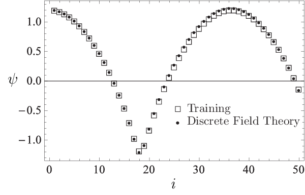
The training data are plotted in Fig. 2 using empty square markers. It is a time sequence generated by the nonlinear ODE
| (13) |
with initial conditions and Here denote . The Lagrangian density for the system is
| (14) |
The optimizer for training the discrete Lagrangian density is Newton’s algorithm with step-lengths reduced according to the amplitude of loss function. The discrete Lagrangian density is trained until the loss function on is less than , then it is served. Plotted in Fig. 2 using solid circle markers are the predicted time sequence using the initial conditions of the training data, i.e., and The predicted sequence and the training sequence are barely distinguishable in the figure.
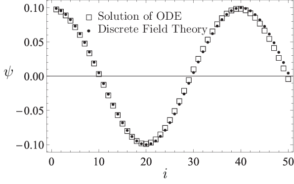
The learned discrete field theory is then served with two sets of new initial conditions, and the predicted time sequences are plotted using solid circle markers in Fig. 3 and Fig. 4 against the time sequences solved for from the nonlinear ODE (13). The predicted sequence in Fig. 3 starts at , and its dynamic characteristics is significantly different from that of the sequence in Fig. 2. The predicted sequence in Fig. 4 starts at a much smaller amplitude, i.e., , and shows the behavior of linear oscillation, in contrast with the strong nonlinearity of the sequence in Fig. 2 and the mild nonlinearity of the sequence in Fig. 3. The agreement between the predictions of the learned discrete field theory and the accurate solutions of the nonlinear ODE (13) is satisfactory. These numerical results demonstrate that the proposed algorithms for machine learning and serving of discrete field theories are effective in terms of capturing the fundamental structure and predicting the complicated dynamical behavior of the physical system.

Example 2.
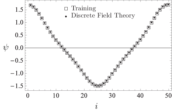
The training data are plotted in Fig. 5 using empty square markers. It is a time sequence generated by the nonlinear ODE
| (15) |
with initial conditions and The Lagrangian for the system is
| (16) | ||||
| (17) |
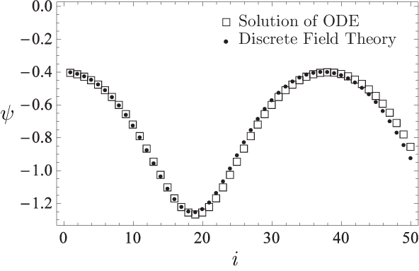
where is a nonlinear potential plotted in Fig. 6. The training sequence represents a nonlinear oscillation in the potential well between . The trained discrete Lagrangian density is accepted when the loss function on the training sequence is less than . The predicted sequence (solid circles in Fig. 5) by the serving algorithm from the learned discrete field theory agrees very well with the training sequence .
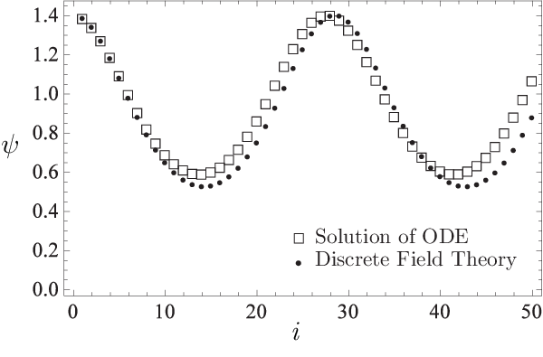
The learned discrete field theory predicts two very different types of dynamical sequences shown in Fig. 7 and Fig. 8. The predicted sequences are plotted using solid circle markers and the sequences accurately solved for from the nonlinear ODE (15) are plotted using empty square markers. The sequence predicted in Fig. 7 is a nonlinear oscillation in the small potential well between and on the right of Fig. 6, and the sequence predicted in Fig. 8 is a nonlinear oscillation in the small potential well between and on the left. For both cases, the predictions of the learned discrete field theory agree with the accurate solutions. Observe that in Fig. 6 the two small potential wells are secondary to the large potential wall between . In Fig. 5 the small-scale fluctuations in the training sequence, which is a nonlinear oscillation in the large potential well, encode the structures of the small potential wells. The training algorithm is able to diagnose and record these fine structures in the learned discrete Lagrangian density, and the serving algorithm correctly predicts the secondary dynamics due to them.

4 Kepler problem
In this section, to further demonstrate the effectiveness of the method developed, I apply it to the Kepler problem, which is concerned with dynamics of planetary orbits in the solar system. Let turn the clock back to 1601, when Kepler inherited the observational data of planetary orbits meticulously collected by his mentor Tycho Brahe. It took Kepler 5 years to discover his first and second laws of planetary motion, and another 78 years before Newton solved the Kepler problem using his laws of motion and universal gravitation (Newton 2008). Assume that we have a set of data similar to that of Kepler, as displayed in Fig. 9. For simplicity, the data are the orbits of the Mercury, Venus, Earth, Mars, Ceres and Jupiter generated by solving Newton’s equation of motion for a planet in the gravity field of the Sun according to Newton’s law of universal gravitation. The spatial and temporal normalization scale-lengths are 1 a.u. and 58.14 days, respectively, and the time-steps of the orbital data is 0.05.


My goal here is not to rediscover Kepler’s laws of planetary motion or Newton’s laws of motion and universal gravitation by machine learning. Instead, I train a discrete field theory from the orbits displayed in Fig. 9 and then serve it to predict new planetary orbits. For this case, the discrete field theory is about a 2D vector field defined on the time grid. Denote the field as , where is the index for the time grid, and and are the 2D coordinates of a planet in the solar system. In terms of the discrete field, the discrete Lagrangian density is a function on
| (18) |
and the DEL is a vector equation with two components,
| (19) | |||
| (20) |
The loss function on a data set is
Akin to the situation in Sec. 3, the serving algorithms preserves exactly an discrete symplectic form defined by
| (21) | |||
| (22) |
To model the discrete Lagrangian density , I use a fully connected neural network with two hidden layers, each of which has 40 neurons with the sigmoid activation function. The network is randomly initialized with a normal distribution, and then trained by the Adam optimizer (Kingma and Ba) until the averaged loss on a single time grid-point is reduced by a factor of relative to its initial value. Starting from the same initial conditions as the training orbits, the serving algorithm of the trained discrete field theory predicts the orbits plotted using red markers in Fig. 10 against the training orbits indicated by green markers. The agreement between the predicted and training orbits shown in the figure validates the discrete field theory learned. To serve it for the purpose of predicting new orbits, let’s consider the scenario of launching a device at the Perihelion of the Earth orbit with an orbital velocity larger than that of the Earth. Four such orbits, labeled by e1, e2, h, and p with and are plotted in Fig. 11 along with the orbit of the Earth, which is the inner most ellipse labeled by e0 with . Orbits plotted using red markers are predictions of the trained discrete field theory, and orbits plotted using blue markers are solutions according to Newton’s laws of motion and gravitation. The agreement is excellent. Orbits e1 and e2 are elliptical, and Orbit p is the parabolic escaping orbit and Orbit h is the hyperbolic escaping orbit.
Similar study is carried out for the orbits initiated from the Perihelion of the Mercury orbit with an orbital velocities larger than that of the Mercury. Four such orbits are shown in Fig. 12 using the same plotting markers and labels as in Fig. 11. The inner most elliptical orbit is that of the Mercury with . The orbit velocities at the Perihelion of the other four orbits are , Again, the the predictions of the trained discrete field theory agree very well with those of Newton’s laws.


It is remarkable that the trained discrete field theory correctly predicts the parabolic and hyperbolic escaping orbits, even though the training orbits are all elliptical, see Figs. 9 and 10. Historically, Kepler argued that escaping orbits and elliptical orbits are governed by different laws. It was Newton who discovered or “learned” the dependency of the gravitational field from Kepler’s laws of planetary motion and Tycho Brahe’s data, and unified the elliptical orbits and escaping orbits under the same law of physics. Most of the studies physicists have been doing since then is applying Newton’s methodology to other physical phenomena. The results displayed in Figs. 11 and 12 show that the machine learning and serving algorithms solve the Kepler problem in terms of correctly prediction planetary orbits without knowing or learning Newton’s laws of motion and universal gravitation.
To complete this section, a few footnotes are in order. (i) There exist small discrepancies between the predictions from the learned discrete field theory and Newton’s laws in Figs. 11 and 12 when . This is because no training orbit in this domain was provided to the learning algorithm. The orbits predicted there are thus less accurate. (ii) The study presented is meant to be a proof of principle. Practical factors, such as three-body effects, are not included. Nevertheless, the method itself is robust against variations of the governing laws of physics, because the method does not require any knowledge of the laws of physics other than the fundamental assumption that the governing laws are field theories. In particular, the learning and serving algorithms for planetary orbits described above do not assume or make use of Newton’s equation of motion and Newton’s law of universal gravitation. Therefore, when the effects of special relativity or general relativity are important, the algorithms are valid without modification. Further study will be reported in the future.
5 Conclusions and discussion
In this paper, a method for machine learning and serving of discrete field theories in physics is developed. The learning algorithm trains a discrete field theory from a set of observational data of the field on a spacetime lattice, and the serving algorithm employs the learned discrete field theory to predict new observations of the field for given new boundary and initial conditions.
The algorithm does not attempt to capture statistical properties of the training data, nor does it try to discover differential equations that govern the training data. Instead, it learns a discrete field theory that underpins the observed field. Because the learned field theory is discrete, it overcomes the difficulties associated with the learning of continuous theories. Compared with continuous field theories, discrete field theories can be served more easily and with improved long-term accuracy and fidelity. The serving algorithm of discrete field theories belongs to the family of structure-preserving geometric algorithms (Feng 1985; Sanz-Serna and Calvo 1994; Marsden et al. 1998; Marsden and West 2001; Hairer et al. 2006; Qin and Guan 2008; Qin et al. 2009; Li et al. 2011; Squire et al. 2012a; Squire et al. 2012b; Squire et al. 2012c; Xiao et al. 2013; Zhang et al. 2014; Zhou et al. 2014; He et al. 2015; Xiao et al. 2015a; Xiao et al. 2015b; Ellison et al. 2015; Qin et al. 2016; He et al. 2016; Xiao et al. 2016; Zhang et al. 2016; Wang et al. 2016; Xiao et al. 2017; Burby 2017; Chen et al. 2017; Zhou et al. 2017; He et al. 2017; Burby and Ellison 2017; Kraus et al. 2017; Xiao et al. 2018; Ellison et al. 2018; Xiao et al. 2019; Xiao and Qin 2019a; Xiao and Qin 2019b; Glasser and Qin 2019a; Shi et al. 2019; Xiao and Qin 2019c), which have been proven to be superior to the conventional algorithms based on discretization of differential equations. The demonstrated advantages of discrete field theories relative to continuous theories in terms of machine learning compatibility are consistent with Bostrom’s simulation hypothesis. The synergy between artificial intelligence and the concept of discrete universe may bring pleasant surprises.
Finally, I should emphasize that no machine learning algorithm is meaningful or effective without presumptions. The algorithms developed here certainly do not apply to any given set of data. The data relevant to the present study are assumed to be observations of physical fields in the spacetime governed by field theories.
However, the existence of a governing field theory is the only physical assumption required. Laws of physics in specific forms, such as Newton’s laws of motion and gravity, special relativity and general relativity, and Schrödinger’s equation, are not needed for the machine learning and serving algorithms of discrete field theories to be effective in terms of correctly predicting observations.
Acknowledgements.
This research was supported by the U.S. Department of Energy (DE-AC02-09CH11466). I thank Alexander S. Glasser, Yichen Fu, Michael Churchill, George Wilkie, and Nick McGreivy for fruitful discussions.References
- Narendra and Parthasarathy (1990) K. S. Narendra and K. Parthasarathy, IEEE Transactions on Neural Networks 1, 4 (1990).
- Narendra and Parthasarathy (1992) K. S. Narendra and K. Parthasarathy, Int. J. Approx. Reasoning 6, 109 (1992).
- Ramacher (1993) U. Ramacher, Neural Networks 6, 547 (1993).
- Howse et al. (1995) J. W. Howse, C. T. Abdallah, and G. L. Heileman, in Advances in Neural Information Processing Systems 8 (1995) pp. 274–280.
- Wilde (1993) P. D. Wilde, Physical Review E 47, 1392 (1993).
- E (2017) W. E, Communications in Mathematics and Statistics 5, 1 (2017).
- Chen et al. (2018) T. Q. Chen, Y. Rubanova, J. Bettencourt, and D. Duvenaud, in Advances in Neural Information Processing Systems, Vol. 31 (2018) pp. 6572–6583.
- Haber and Ruthotto (2018) E. Haber and L. Ruthotto, Inverse Problems 34, 014004, 22 (2018).
- Wroblewski et al. (1997) D. Wroblewski, G. Jahns, and J. Leuer, Nuclear Fusion 37, 725 (1997).
- Vannucci et al. (1999) A. Vannucci, K. Oliveira, and T. Tajima, Nuclear Fusion 39, 255 (1999).
- Yoshino (2003) R. Yoshino, Nuclear Fusion 43, 1771 (2003).
- Kates-Harbeck et al. (2019) J. Kates-Harbeck, A. Svyatkovskiy, and W. Tang, Nature 568, 526 (2019).
- Wu et al. (2018) J.-L. Wu, H. Xiao, and E. Paterson, Phys. Rev. Fluids 3, 074602 (2018).
- Bar-Sinai et al. (2019) Y. Bar-Sinai, S. Hoyer, J. Hickey, and M. P. Brenner, Proceedings of the National Academy of Sciences 116, 15344 (2019).
- Han et al. (2019) J. Han, C. Ma, Z. Ma, and W. E, Proceedings of the National Academy of Sciences 116, 21983 (2019).
- Dissanayake and Phan-Thien (1994) M. W. M. G. Dissanayake and N. Phan-Thien, Communications in Numerical Methods in Engineering 10, 195 (1994).
- Meade and Fernández (1994a) A. J. Meade, Jr. and A. A. Fernández, Mathematical and Computer Modelling 19, 1 (1994a).
- Meade and Fernández (1994b) A. J. Meade, Jr. and A. A. Fernández, Mathematical and Computer Modelling 20, 19 (1994b).
- Lagaris et al. (1998) I. E. Lagaris, A. Likas, and D. I. Fotiadis, IEEE Transactions on Neural Networks 9, 987 (1998).
- Bailer-Jones et al. (1998) C. A. L. Bailer-Jones, D. J. C. MacKay, and P. J. Withers, Network: Computation in Neural Systems 9, 531 (1998).
- Long et al. (2019) Z. Long, Y. Lu, and B. Dong, Journal of Computational Physics 399, 108925 (2019).
- Carleo and Troyer (2017) G. Carleo and M. Troyer, Science 355, 602 (2017).
- Nomura et al. (2017) Y. Nomura, A. S. Darmawan, Y. Yamaji, and M. Imada, Physical Review B 96, 205152 (2017).
- Bongard and Lipson (2007) J. Bongard and H. Lipson, Proceedings of the National Academy of Sciences 104, 9943 (2007).
- Schmidt and Lipson (2009) M. Schmidt and H. Lipson, Science 324, 81 (2009).
- Brunton et al. (2016) S. L. Brunton, J. L. Proctor, and J. N. Kutz, Proceedings of the National Academy of Sciences 113, 3932 (2016).
- Rudy et al. (2017) S. H. Rudy, S. L. Brunton, J. L. Proctor, and J. N. Kutz, Science Advances 3, e1602614 (2017).
- Schaeffer (2017) H. Schaeffer, Proceedings of the Royal Society A: Mathematical, Physical and Engineering Sciences 473, 20160446 (2017).
- Baydin et al. (2017) A. G. Baydin, B. A. Pearlmutter, A. A. Radul, and J. M. Siskind, J. Mach. Learn. Res. 18, 153:1 (2017).
- Raissi (2018) M. Raissi, Journal of Machine Learning Research 19, 1 (2018).
- Cranmer et al. (2019a) M. D. Cranmer, R. Xu, P. Battaglia, and S. Ho, “Learning symbolic physics with graph networks,” (2019a), 1909.05862v2 .
- Gelß et al. (2019) P. Gelß, S. Klus, J. Eisert, and C. Schütte, Journal of Computational and Nonlinear Dynamics 14, 061006 (2019).
- Raissi et al. (2019) M. Raissi, P. Perdikaris, and G. Karniadakis, Journal of Computational Physics 378, 686 (2019).
- Wu et al. (2019) K. Wu, T. Qin, and D. Xiu, “Structure-preserving method for reconstructing unknown Hamiltonian systems from trajectory data,” (2019), 1905.10396v1 .
- Lutter et al. (2019) M. Lutter, C. Ritter, and J. Peters, “Deep Lagrangian networks: Using physics as model prior for deep learning,” (2019), 1907.04490v1 .
- Bertalan et al. (2019) T. Bertalan, F. Dietrich, I. Mezić, and I. G. Kevrekidis, “On learning Hamiltonian systems from data,” (2019), 1907.12715v2 .
- Greydanus et al. (2019) S. Greydanus, M. Dzamba, and J. Yosinski, “Hamiltonian neural networks,” (2019), 1906.01563v3 .
- Zhong et al. (2019) Y. D. Zhong, B. Dey, and A. Chakraborty, “Symplectic ode-net: Learning Hamiltonian dynamics with control,” (2019), 1909.12077v1 .
- Sanchez-Gonzalez et al. (2019) A. Sanchez-Gonzalez, V. Bapst, K. Cranmer, and P. Battaglia, “Hamiltonian graph networks with ode integrators,” (2019), 1909.12790v1 .
- Chen et al. (2019) Z. Chen, J. Zhang, M. Arjovsky, and L. Bottou, “Symplectic recurrent neural networks,” (2019), 1909.13334v1 .
- Toth et al. (2019) P. Toth, D. J. Rezende, A. Jaegle, S. Racanière, A. Botev, and I. Higgins, “Hamiltonian generative networks,” (2019), 1909.13789v1 .
- Shanahan et al. (2018) P. E. Shanahan, D. Trewartha, and W. Detmold, Physical Review D 97, 094506 (2018).
- Noé et al. (2019) F. Noé, S. Olsson, J. Köhler, and H. Wu, Science 365, eaaw1147 (2019).
- Halverson et al. (2019) J. Halverson, B. Nelson, and F. Ruehle, Journal of High Energy Physics 2019, 3 (2019).
- Cranmer et al. (2019b) K. Cranmer, S. Golkar, and D. Pappadopulo, “Inferring the quantum density matrix with machine learning,” (2019b), 1904.05903v1 .
- Feng (1985) K. Feng, in the Proceedings of 1984 Beijing Symposium on Differential Geometry and Differential Equations, edited by K. Feng (Science Press, 1985) pp. 42–58.
- Sanz-Serna and Calvo (1994) J. M. Sanz-Serna and M. P. Calvo, Numerical Hamiltonian Problems (Chapman and Hall, London, 1994).
- Marsden et al. (1998) J. E. Marsden, G. W. Patrick, and S. Shkoller, Communications in Mathematical Physics 199, 351 (1998).
- Marsden and West (2001) J. E. Marsden and M. West, Acta Numerica 10, 357 (2001).
- Hairer et al. (2006) E. Hairer, C. Lubich, and G. Wanner, Geometric Numerical Integration: Structure-preserving Algorithms for Ordinary Differential Equations, Vol. 31 (Springer, 2006).
- Qin and Guan (2008) H. Qin and X. Guan, Physical Review Letters 100, 035006 (2008).
- Qin et al. (2009) H. Qin, X. Guan, and W. M. Tang, Physics of Plasmas 16, 042510 (2009).
- Li et al. (2011) J. Li, H. Qin, Z. Pu, L. Xie, and S. Fu, Physics of Plasmas 18, 052902 (2011).
- Squire et al. (2012a) J. Squire, H. Qin, and W. M. Tang, Geometric Integration of the Vlasov-Maxwell System with a Variational Particle-in-cell Scheme, Tech. Rep. PPPL-4748 (Princeton Plasma Physics Laboratory, 2012).
- Squire et al. (2012b) J. Squire, H. Qin, and W. M. Tang, Physics of Plasmas 19, 084501 (2012b).
- Squire et al. (2012c) J. Squire, H. Qin, and W. M. Tang, Physics of Plasmas 19, 052501 (2012c).
- Xiao et al. (2013) J. Xiao, J. Liu, H. Qin, and Z. Yu, Physics of Plasmas 20, 102517 (2013).
- Zhang et al. (2014) R. Zhang, J. Liu, Y. Tang, H. Qin, J. Xiao, and B. Zhu, Physics of Plasmas 21, 032504 (2014).
- Zhou et al. (2014) Y. Zhou, H. Qin, J. W. Burby, and A. Bhattacharjee, Physics of Plasmas 21, 102109 (2014).
- He et al. (2015) Y. He, H. Qin, Y. Sun, J. Xiao, R. Zhang, and J. Liu, Physics of Plasmas 22, 124503 (2015).
- Xiao et al. (2015a) J. Xiao, H. Qin, J. Liu, Y. He, R. Zhang, and Y. Sun, Physics of Plasmas 22, 112504 (2015a).
- Xiao et al. (2015b) J. Xiao, J. Liu, H. Qin, Z. Yu, and N. Xiang, Physics of Plasmas 22, 092305 (2015b).
- Ellison et al. (2015) C. L. Ellison, J. M. Finn, H. Qin, and W. M. Tang, Plasma Physics and Controlled Fusion 57, 054007 (2015).
- Qin et al. (2016) H. Qin, J. Liu, J. Xiao, R. Zhang, Y. He, Y. Wang, Y. Sun, J. W. Burby, L. Ellison, and Y. Zhou, Nuclear Fusion 56, 014001 (2016).
- He et al. (2016) Y. He, Y. Sun, H. Qin, and J. Liu, Physics of Plasmas 23, 092108 (2016).
- Xiao et al. (2016) J. Xiao, H. Qin, P. J. Morrison, J. Liu, Z. Yu, R. Zhang, and Y. He, Physics of Plasmas 23, 112107 (2016).
- Zhang et al. (2016) R. Zhang, H. Qin, Y. Tang, J. Liu, Y. He, and J. Xiao, Physical Review E 94, 013205 (2016).
- Wang et al. (2016) Y. Wang, J. Liu, and H. Qin, Physics of Plasmas 23, 122513 (2016).
- Xiao et al. (2017) J. Xiao, H. Qin, J. Liu, and R. Zhang, Physics of Plasmas 24, 062112 (2017).
- Burby (2017) J. W. Burby, Physics of Plasmas 24, 032101 (2017).
- Chen et al. (2017) Q. Chen, H. Qin, J. Liu, J. Xiao, R. Zhang, Y. He, and Y. Wang, Journal of Computational Physics 349, 441 (2017).
- Zhou et al. (2017) Z. Zhou, Y. He, Y. Sun, J. Liu, and H. Qin, Physics of Plasmas 24, 052507 (2017).
- He et al. (2017) Y. He, Z. Zhou, Y. Sun, J. Liu, and H. Qin, Physics Letters A 381, 568 (2017).
- Burby and Ellison (2017) J. W. Burby and C. L. Ellison, Physics of Plasmas 24, 110703 (2017).
- Kraus et al. (2017) M. Kraus, K. Kormann, P. J. Morrison, and E. Sonnendrücker, Journal of Plasma Physics 83, 905830401 (2017).
- Xiao et al. (2018) J. Xiao, H. Qin, and J. Liu, Plasma Science and Technology 20, 110501 (2018).
- Ellison et al. (2018) C. L. Ellison, J. M. Finn, J. W. Burby, M. Kraus, H. Qin, and W. M. Tang, Physics of Plasmas 25, 052502 (2018).
- Xiao et al. (2019) J. Xiao, H. Qin, Y. Shi, J. Liu, and R. Zhang, Physics Letters A 383, 808 (2019).
- Xiao and Qin (2019a) J. Xiao and H. Qin, Nuclear Fusion 59, 106044 (2019a).
- Xiao and Qin (2019b) J. Xiao and H. Qin, Computer Physics Communications 241, 19 (2019b).
- Glasser and Qin (2019a) A. S. Glasser and H. Qin, “The geometric theory of charge conservation in particle-in-cell simulations,” (2019a), 1910.12395v1 .
- Shi et al. (2019) Y. Shi, Y. Sun, Y. He, H. Qin, and J. Liu, Numerical Algorithms (2019), 10.1007/s11075-018-0636-6.
- Xiao and Qin (2019c) J. Xiao and H. Qin, “Structure-preserving geometric particle-in-cell algorithm suppresses finite-grid instability – comment on "finite grid instability and spectral fidelity of the electrostatic particle-in-cell algorithm" by Huang et al.” (2019c), 1904.00535v1 .
- de Maupertuis (1744) P. de Maupertuis, Mém. As. Sc. Paris , 417 (1744).
- de Maupertuis (1746) P. de Maupertuis, Mém. Ac. Berlin , 267 (1746).
- Bostrom (2003) N. Bostrom, The Philosophical Quarterly 53, 243 (2003).
- Beane et al. (2014) S. R. Beane, Z. Davoudi, and M. J. Savage, Eur. Phys. J. A50, 148 (2014).
- Glasser and Qin (2019b) A. S. Glasser and H. Qin, “Lifting spacetime’s Poincaré symmetries,” (2019b), 1902.04395v1 .
- Glasser and Qin (2019c) A. S. Glasser and H. Qin, “Restoring Poincaré symmetry to the lattice,” (2019c), 1902.04396v1 .
- (90) D. P. Kingma and J. Ba, “Adam: A method for stochastic optimization,” 1412.6980v9 .
- Davoudi and Savage (2012) Z. Davoudi and M. J. Savage, Phys. Rev. D 86, 054505 (2012).
- Newton (2008) I. Newton, in The Mathematical Papers of Isaac Newton, Volume IV, 1684 -1691 (Cambridge University Press, 2008) p. 30.