Motion of Charged Particles around a
Scalarized Black Hole in Kaluza-Klein Theory

The two horizons of the rotating dyonic black hole are given by $\Delta=0$. The horizons are present for

This yields $M_{K}^{2}\geq a^{2}$, which is the same condition as for the original Kerr spacetime to have horizons. It is interesting to the study the extremal case with a single degenerate horizon. In Einstein-Maxwell theory the surface of extreme solutions, formed by the scaled global charges $\frac{J}{M^{2}}$, $\frac{Q}{M}$ and $\frac{P}{M}$, is a sphere. In Kaluza-Klein theory this surface is not smooth but made up of two parts as shown in figure 1 (see also Rasheed:1995zv).

The first surface (blue in figure 1) emerges from the condition for a single degenerate horizon $M^{2}=P^{2}+Q^{2}+a^{2}-\Sigma^{2}$, which leads to $M_{K}=a^{2}$ and therefore boosting the extremal Kerr solution will lead to the blue surface.

The second surface (green in figure 1) represents the special case $M^{2}+\Sigma^{2}=P^{2}+Q^{2}$. Then $a=0$ and $M_{K}=0$ but $\frac{a}{M_{K}}\leq 1$, so that the angular momentum $J$ may be non-zero. This can be seen by taking the extremal limit $\beta\rightarrow\infty$ of the boosted solutions, thus

Then we have

So any non-rotating dyonic solution with fixed $M,P,Q$ on this part of the surface can be given angular momentum $J\leq PQ$ and it will still remain extremal. In Einstein-Maxwell adding angular momentum to an extremal black hole would lead to a naked singularity.

In this article we will concentrate on the special case

where the metric is

and the non-zero components of the electromagnetic vector potential are

The metric possesses a singularity at $r_{S}=\sqrt{2\lvert J\cos\theta\rvert}$, which is hidden behind an event horizon at $r_{H}=M$ if $J<\frac{M^{2}}{2}$. As for all solutions on the green surface, there is no ergoregion.

In the extremal case the dilaton field is

which means that $\sigma=0$ for $J=0$ and also $\sigma=0$ in the equatorial plane $\theta=\frac{\pi}{2}$.

Let us investigate the motion of electrically charged particles around the extremal dyonic black hole described by the equation (26). As described in Maki:1992up; Pris:1995; Rahaman:2003wv we will take into account the effects of the dilaton field. The Hamiltonian for a charged particle with the electric charge $q$ is

where the parameter $\beta$ describes the coupling to the dilaton field $\sigma$. The mass shell condition is in this case

The Hamilton-Jacobi equation is

with $p_{\mu}=\frac{\partial S}{\partial x^{\mu}}$ and an affine parameter $\lambda$ along the trajectory of the test particle. To solve equation (32) we use the following ansatz for the action

where $E$ is the energy and $L$ is the angular momentum of the test particle. The parameter $\delta=m^{2}$ describes the particle’s mass and is $1$ for particles and $0$ for light. With this ansatz the Hamilton-Jacobi equation becomes

Inserting the metric (26), the vector potential (28) and the dilaton field (29) yields

Now we have to separate the above equation to get (the derivatives of) the unknown functions $S_{\theta}(\theta)$ and $S_{r}(r)$. This is possible in three cases:

1. 1.

   For photons with $\delta=0$ and $q=0$, equation (35) simplifies to

   $$\frac{(4J^{2}-r^{4})E^{2}}{(r-M)^{2}}-\frac{4JEL}{r-M}+\frac{L^{2}}{\sin^{2}\!\theta}+\left(\frac{\partial S_{\theta}(\theta)}{\partial\theta}\right)^{2}+(r-M)^{2}\left(\frac{\partial S_{r}(r)}{\partial r}\right)^{2}=0\,.$$

   (36)

2. 2.

   For a non-rotating black hole with $J=0$, equation (35) yields

   $$\delta r^{2}-\frac{r^{4}}{(r-M)^{2}}\left(-\frac{Mq}{\sqrt{2}r}-E\right)^{2}+\frac{1}{\sin^{2}\!\theta}\left(L-\frac{Mq}{\sqrt{2}}\cos\theta\right)^{2}+\left(\frac{\partial S_{\theta}(\theta)}{\partial\theta}\right)^{2}+(r-M)^{2}\left(\frac{\partial S_{r}(r)}{\partial r}\right)^{2}=0\,.$$

   (37)

3. 3.

   For charged particles in the equatorial plane $\theta=\frac{\pi}{2}$, equation (35) becomes

   $$\delta r^{2}-\frac{\left(r^{4}-4J^{2}\right)\left(qM\sqrt{2}+2Er\right)^{2}}{4r^{2}(r-M)^{2}}-\frac{2J\left(qM\sqrt{2}+2Er\right)\left(Jq\sqrt{2}+Lr\right)}{(r-M)r^{2}}+\frac{\left(Jq\sqrt{2}+Lr\right)^{2}}{r^{2}}+(r-M)^{2}\left(\frac{\partial S_{r}(r)}{\partial r}\right)^{2}=0\,.$$

   (38)

So far we have described the particle motion in the four-dimensional Rasheed spacetime, which respresents a scalarized black hole. Since most scalarized black holes are given as a numerical solution, it is interesting to have some insight on the analytical side.

On the other hand, one has to take into account that the four-dimensional Rasheed spacetime is a solution in Kaluza-Klein theory, which is obtained from a five-dimensional spacetime by dimensional reduction. One could argue that in this framework, the Hamilton-Jacobi equation for the four-dimensional problem, does not correctly describe the particle motion. Instead the equation of motion in the five-dimensional metric has to be considered Kovacs:1984qx–Kerner:2000iz. Here the dilatonic force yields new terms in the equations of motion.

In the following we will prove that in the above special cases, the particle motion is correctly described by the Hamilton-Jacobi equation for the four-dimensional problem.

In case 1, all new terms entering the equations of motion vanish since $\delta=0$ and $q=0$, compare Kovacs:1984qx–Liu:1997fg. In case 2, the dilaton field vanishes everywhere, because $J=0$. In case three, the dilaton field vanishes in the equatorial plane since $\theta=\frac{\pi}{2}$. However, derivatives of the dilaton field enter the equations of motion in the five-dimensional spacetime Kovacs:1984qx–Liu:1997fg. Therefore it has to be checked, if there are effects due to the dilaton in the equatorial plane.

The four-dimensional black hole spacetime ${\mathrm{d}}s^{2}_{(4)}$ of Rasheed (see equation (1)) can be obtained from the five-dimensional metric

The motion of a test particle in this metric is described by the Hamilton-Jacobi equation

with $\tilde{p}_{\mu}=\frac{\partial S_{5}}{\partial x^{\mu}}$. To solve equation (40) we propose the ansatz

where $K$ is a constant of motion corresponding to the momentum in the direction if the fifth dimension $x^{5}=w$. With this ansatz equation (40) becomes

Inserting the metric functions of the five-dimensional metric into equation (42) results in a long and complicated expression, which we will not display here. Setting then $\theta=\frac{\pi}{2}$ simplifies the equation to

It can be shown that equation (43) is the same as the Hamilton-Jacobi equation (38) for a charged particle in the equatorial plane of the four-dimensional spacetime if we make the identifications

which result in the relation

The same relation without the factor 2 was found in Liu:1997fg, Kerner:2000iz. Here the factor 2 is due to the fact that there is an additional factor 2 in front of the vector field $A_{\mu}$ in the five-dimensional Rasheed metric, which is not present in the metric in Liu:1997fg, Kerner:2000iz. Therefore in the equatorial plane of the extreme Rasheed metric, the Hamilton-Jacobi equation from the four-dimensional particle motion agrees with the Hamilton-Jacobi equation from the five-dimensional problem and correctly describes the motion of test particles.

In this article we are interested in the motion of charged particles around an extremal rotating dyonic black hole in Kaluza-Klein theory; thus, we will consider the third case and set $\theta=\frac{\pi}{2}$ from now on. The equations of motion in the equatorial plane can be derived from the action $S$ (33)

To simplify the equations of motion we used dimensionless quantities equivalent to setting $M=1$

and we also applied the Mino-time Mino:2003yg $\gamma$ with ${\mathrm{d}}\lambda=r^{3}{\mathrm{d}}\gamma$. The function $R(r)$ in equation (46) is a polynomial of order $6$ with the coefficients

In general the equations of motion are of hyperelliptic type. However, in the special case of uncharged particles $q=0$ the equations of motion reduce to elliptic type (note that ${\mathrm{d}}\lambda=r{\mathrm{d}}\gamma$ in this case)

where

Both in the hyperelliptic and the elliptic case the equations of motion can be solved analytically as shown in section IV.

The $\phi$-equation (47) determines the azimuthal motion. ${\mathrm{d}}\phi/{\mathrm{d}}\gamma$ vanishes if

or

At these radii the test particles change their direction, which leads to interesting orbits, see section IV.4. A similar effect is usually observed at the ergoregion of a black hole. However, in this spacetime an ergoregion does not exist. The radii at which the angular direction changes were called turnaround boundaries in Diemer:2013fza.

The radial equation of motion determines the type of the orbits, because its zeros are the turning points of the orbit. Particle motion is allowed for $R(r)\geq 0$ only. Here we are interested in the real positive zeros. To study the possible orbits, parametric diagrams and effective potentials can be constructed from the polynomial $R(r)$. First we will give a list of the possible orbit types:

1. 1.

   Bound orbits (BO) with $r\in[r_{1},r_{2}]$ exist for $r_{1,2}>r_{H}$ and also for $r_{1,2}<r_{H}$ hidden behind the event horizon.

2. 2.

   Many-world bound orbits (MBO) with $r\in[r_{1},r_{2}]$ and $r_{1}<r_{H}<r_{2}$, where the particle crosses the horizon several times. Each time the horizon is crossed twice the particle enters another universe.

3. 3.

   Escape orbits (EO) with $r\in[r_{1},\infty)$ and $r_{1}>r_{H}$, where the test particle (or light) escapes the gravity of the black hole.

4. 4.

   Two-world escape orbits (TWEO) with $r\in[r_{1},\infty)$ and $r_{1}<r_{H}$, where the particle crosses the horizon twice and enters another universe.

The number of zeros of $R(r)$ for a set of parameters is closely related to the possible orbit types. If double zeros occur, i.e. $R(r)=0$ and $\frac{{\mathrm{d}}R}{{\mathrm{d}}r}=0$, the number of zeros changes. We plot these two conditions as a parameterplot of $E$ and $L$ to see nine regions with different numbers of real positive zeros. An example of a parameterplot is shown in figure 2. There is one real positive zero in region I, two zeros in region II, three zeros in the regions III and IV, four zeros in the regions V and VI, five zeros in the regions VII and VII, and six zeros in region IX. Two regions may have the same number of positive real zeros; however, there are different types of possible orbits.

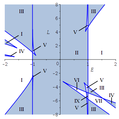
The orbit types in each region can be determined with the help of effective potentials. We define an effective potential consisting of two parts $V^{\pm}$ by

and therefore

In the case of uncharged photons $\delta=q=0$ the effective potentials simplify to

At the horizon $r_{H}=1$ the two effective potentials meet at $E=-\frac{q}{\sqrt{2}}$. Here $R(r=r_{H},E=-\frac{q}{\sqrt{2}})=0$ and a circular orbit exists directly on the horizon. Furthermore, the two potentials meet at a point behind the horizon, which can be calculated by

For $r\rightarrow 0$ both potentials diverge. Additionally for $r\rightarrow\sqrt{2|J|}$, the potential $V_{+}$ diverges if $JL<0$ and $V_{-}$ diverges if $JL>0$. However, the latter divergency has no effect on the orbits, since the equations of motion remain smooth and therefore we will not show this divergency in the plots of the effective potentials . At $r\rightarrow\infty$ the potentials $V^{\pm}$ aproach $\mp\sqrt{\delta}$ asymptotically. We find the following symmetries

In the Schwarzschild spacetime the positive root of the effective potential is always $V_{+}\geq 0$ and the negative root $V_{-}\leq 0$. There is no classical interpretation for particles with negative energies; however, in quantum field theory they can be associated with antiparticles Deruelle:1974zy. Note that in contrast to the Schwarzschild spacetime, here the positive root $V_{+}$ can be negative, which can allow particles with negative energies. In Christodoulou:1972kt; Denardo:1973 the region for particles with negative energies was described as a “generalized ergosphere”, where energy may be extracted. Also the negative root $V_{-}$ can be positive in this spacetime. To find a bound which separates particles and antiparticles, one can consider equation (48) which describes the coordinate time $t$. Time should run forward for particles and backwards for antiparticles. Solving the $t$-equation for $E$ will give a lower energy bound for particles, which can be negative in the “generalized ergosphere”.

Some examples of the potentials are depicted in figure 3. We also plot the energy $E_{\rm turn}$ (equation (65)) where the test particles changes angular direction.

Taking all the information from the parameterplots and the effective potentials into account, we determine the possible orbits for charged particles in the spacetime of an extremal black hole in Kaluza-Klein theory. An overview of the regions and the corresponding orbit types can be found in table 1 and the following list.

1. 1.

   Region I: The polynomial $R$ has one zero $r_{1}<r_{H}$ and the corresponding orbit is a TWEO.

2. 2.

   Region II: $R$ has two zeros $r_{1}<r_{H}$ and $r_{2}>r_{H}$. The corresponding orbit is a MBO.

3. 3.

   Region III: $R$ has three zeros $r_{1}<r_{H}$ and $r_{2},r_{3}>r_{H}$. A MBO and a EO exist.

4. 4.

   Region IV: $R$ has three zeros $r_{1},r_{2}<r_{H}$ and $r_{3}>r_{H}$. A BO hidden behind the horizon and a TWEO exist.

5. 5.

   Region V: $R$ has four zeros $r_{1}<r_{H}$ and $r_{2},r_{3},r_{4}>r_{H}$. Here a MBO and a BO exist.

6. 6.

   Region VI: $R$ has four zeros $r_{1},r_{2},r_{3}<r_{H}$ and $r_{4}>r_{H}$. A BO hidden behind the horizon and a MBO exist.

7. 7.

   Region VII: $R$ has five zeros $r_{1},r_{2},r_{3}<r_{H}$ and $r_{4},r_{5}>r_{H}$. A BO hidden behind the horizon, a MBO and a EO exist.

8. 8.

   Region VIII: $R$ has five zeros $r_{1},r_{2},r_{3},r_{4},r_{5}<r_{H}$. Two BOs hidden behind the horizon and a TWEO exist.

9. 9.

   Region IX: $R$ has six zeros $r_{1},r_{2},r_{3}<r_{H}$ and $r_{4},r_{5},r_{6}>r_{H}$. A BO hidden behind the horizon, a MBO and a second BO outside the black hole exist.

In the special case of massless particles with $\delta=q=0$, only the regions I, II, III and IV exist. For massless particles in region II, $R$ possesses a double zero at $r_{H}=1$ and the energy is always $E=0$, here light moves on a circular orbit directly on the horizon.

Let us now investigate under which conditions an orbit terminates at the singularity $r_{S}$. At the singularity, the polynomial $R$ has the value

Therefore in the case $J\neq 0$ and $q\neq 0$ particles can never reach the singularity. If $J=0$ or $q=0$ we have $R(r_{S})=0$, but then $r_{S}=0$ is a local maximum of $R$, so that test particles can never reach that point.

1. 1.

   If $J=0$ then $R^{\prime}(r=0)=0$ and $R^{\prime\prime}(r=0)=-L^{2}$.

2. 2.

   If $q=0$ then $R^{\prime}(r=0)=0$ and $R^{\prime\prime}(r=0)=-2(2EJ+L)^{2}$.

If additionally $L=0$ in the first case or $J=L=0$ in the second case then $r_{S}=0$ is an inflection point. The effective potentials show that the singularity is guarded by a potential barrier which makes it impossible to find orbits that reach $r_{S}=0$. Only in the special case $J=L=q=\delta=0$ particles can reach the singularity. Here in fact all orbits end in the singularity.

In Collodel:2017end static orbits in axisymmetric rotating spacetimes were discovered. Under certain conditions there is a ring of points in the equatorial plane where particles remain at rest. We will show that these orbits also exist in the Rasheed spacetime.

A particle is at rest at a certain point if

From this we can calculate the radius and the energy of the particle at rest

At $r_{\rm rest}$ the effective potentials (equation (68)) intersect with the turnaround boundary (equation (65)) and the particle is at rest at the pericenter or apocenter of its orbit. If the turnaround boundary intersects with the local minimum of one of the effective potentials, i.e. if

the particle remains at rest at all times, this is called the static ring. We set $\delta=1$, because then there will be a local minimum in one of the effective potentials for $r>r_{H}$. The above equations then yield

References

- [1] P. T. Chrusciel, J. Lopes Costa and M. Heusler, Living Rev. Rel. 15, 7 (2012)
- [2] C. A. R. Herdeiro and E. Radu, Int. J. Mod. Phys. D 24, no. 09, 1542014 (2015)
- [3] V. Cardoso and L. Gualtieri, Class. Quant. Grav. 33, no. 17, 174001 (2016)
- [4] D. Garfinkle, G. T. Horowitz and A. Strominger, Phys. Rev. D 43, 3140 (1991) Erratum: [Phys. Rev. D 45, 3888 (1992)]. doi:10.1103/PhysRevD.43.3140, 10.1103/PhysRevD.45.3888
- [5] B. Kleihaus, J. Kunz and F. Navarro-Lerida, Phys. Rev. D 69, 081501 (2004) doi:10.1103/PhysRevD.69.081501 [gr-qc/0309082].
- [6] G. W. Gibbons and K. -i. Maeda, Nucl. Phys. B 298, 741 (1988).
- [7] D. Maison, Gen. Rel. Grav. 10, 717 (1979).
- [8] D. Maison, Lect. Notes Phys. 540, 273 (2000).
- [9] A. Chodos and S. L. Detweiler, Gen. Rel. Grav. 14, 879 (1982).
- [10] P. Dobiasch and D. Maison, Gen. Rel. Grav. 14, 231 (1982).
- [11] G. W. Gibbons and D. L. Wiltshire, Annals Phys. 167, 201 (1986) [Erratum-ibid. 176, 393 (1987)].
- [12] V. P. Frolov, A. I. Zelnikov and U. Bleyer, Annalen Phys. 44, 371 (1987).
- [13] P. Breitenlohner, D. Maison and G. W. Gibbons, Commun. Math. Phys. 120, 295 (1988).
- [14] J. H. Horne and G. T. Horowitz, Phys. Rev. D 46, 1340 (1992)
- [15] D. Rasheed, Nucl. Phys. B 454, 379 (1995)
- [16] J. Kunz, D. Maison, F. Navarro-Lerida and J. Viebahn, Phys. Lett. B 639, 95 (2006)
- [17] B. Carter, Commun. Math. Phys. 10, 280 (1968).
- [18] P. Kanti, N. E. Mavromatos, J. Rizos, K. Tamvakis and E. Winstanley, Phys. Rev. D 54, 5049 (1996)
- [19] B. Kleihaus, J. Kunz and E. Radu, Phys. Rev. Lett. 106, 151104 (2011)
- [20] J. L. Blázquez-Salcedo et al., IAU Symp. 324, 265 (2016)
- [21] B. Kleihaus, J. Kunz, S. Mojica and E. Radu, Phys. Rev. D 93, no. 4, 044047 (2016)
- [22] K. D. Kokkotas, R. A. Konoplya and A. Zhidenko, Phys. Rev. D 96, no. 6, 064004 (2017)
- [23] D. D. Doneva and S. S. Yazadjiev, Phys. Rev. Lett. 120, no. 13, 131103 (2018)
- [24] H. O. Silva, J. Sakstein, L. Gualtieri, T. P. Sotiriou and E. Berti, Phys. Rev. Lett. 120, no. 13, 131104 (2018)
- [25] G. Antoniou, A. Bakopoulos and P. Kanti, Phys. Rev. Lett. 120, no. 13, 131102 (2018)
- [26] C. A. R. Herdeiro, E. Radu, N. Sanchis-Gual and J. A. Font, Phys. Rev. Lett. 121, no. 10, 101102 (2018)
- [27] P. V. P. Cunha, C. A. R. Herdeiro and E. Radu, Phys. Rev. Lett. 123, no. 1, 011101 (2019)
- [28] R. A. Konoplya and A. Zhidenko, Phys. Rev. D 100, no. 4, 044015 (2019)
- [29] G. V. Kraniotis and S. B. Whitehouse, Class. Quant. Grav. 20, 4817 (2003)
- [30] G. V. Kraniotis, Class. Quant. Grav. 21, 4743 (2004)
- [31] G. V. Kraniotis, Class. Quant. Grav. 22, 4391 (2005)
- [32] G. V. Kraniotis, Class. Quant. Grav. 24, 1775 (2007)
- [33] R. Fujita and W. Hikida, Class. Quant. Grav. 26, 135002 (2009)
- [34] E. Hackmann, V. Kagramanova, J. Kunz and C. Lämmerzahl, Europhys. Lett. 88, 30008 (2009)
- [35] E. Hackmann, C. Lämmerzahl, V. Kagramanova and J. Kunz, Phys. Rev. D 81, 044020 (2010)
- [36] A. N. Aliev and G. D. Esmer, Phys. Rev. D 87, no. 8, 084022 (2013)
- [37] P. V. P. Cunha, C. A. R. Herdeiro and E. Radu, Phys. Rev. D 98, no. 10, 104060 (2018)
- [38] T. Maki and K. Shiraishi, Class. Quant. Grav. 11, 227 (1994)
- [39] I. Pris, Y. Shnir, and E. Tolkachev, “Test-particle scattering on a magnetically charged dilatonic black hole”, International Centre for Theoretical Physics Technical Report, (1995)
- [40] F. Rahaman, S. B. Dutta Choudhury, R. Mukherji, S. Das and N. Chakraborty, Czech. J. Phys. 53, 115 (2003).
- [41] D. Kovacs, Gen. Rel. Grav. 16, 645 (1984).
- [42] J. Gegenberg and G. Kunstatter, Phys. Lett. A 106, 410 (1984).
- [43] H. Liu and P. S. Wesson, Class. Quant. Grav. 14, 1651 (1997).
- [44] R. Kerner, J. Martin, S. Mignemi and J. W. van Holten, Phys. Rev. D 63, 027502 (2001)
- [45] G. W. Gibbons and C. A. R. Herdeiro, Class. Quant. Grav. 16, 3619 (1999)
- [46] Y. Mino, Phys. Rev. D 67, 084027 (2003)
- [47] V. Diemer and J. Kunz, Phys. Rev. D 89, no. 8, 084001 (2014)
- [48] D. Christodoulou and R. Ruffini, Phys. Rev. D 4, 3552 (1971).
- [49] G. Denardo and R. Ruffini, Phys. Lett. 45 B, 260 (1973).
- [50] N. Deruelle and R. Ruffini, Phys. Lett. 52 B, 437 (1974).
- [51] L. G. Collodel, B. Kleihaus and J. Kunz, Phys. Rev. Lett. 120, no. 20, 201103 (2018)
- [52] C. M. Claudel, K. S. Virbhadra and G. F. R. Ellis, J. Math. Phys. 42, 818 (2001)
- [53] A. Grenzebach, V. Perlick and C. Lämmerzahl, Phys. Rev. D 89, no. 12, 124004 (2014)
- [54] A. Grenzebach, Fund. Theor. Phys. 179, 823 (2015)
- [55] A. Grenzebach, V. Perlick and C. Lämmerzahl, Int. J. Mod. Phys. D 24, no. 09, 1542024 (2015)
- [56] A. Grenzebach, “The Shadow of Black Holes – An Analytic Description”, SpringerBriefs in Physics (Springer, Heidelberg, 2016)
- [57] E. Hackmann, V. Kagramanova, J. Kunz and C. Lämmerzahl, Phys. Rev. D 78, 124018 (2008), Erratum: [Phys. Rev. 79, 029901 (2009)], Addendum: [Phys. Rev. D 79, no. 2, 029901 (2009)]
- [58] E. Hackmann and C. Lämmerzahl, Phys. Rev. D 78, 024035 (2008)
- [59] V. Z. Enolski, E. Hackmann, V. Kagramanova, J. Kunz and C. Lämmerzahl, J. Geom. Phys. 61, 899 (2011)
- [60] V. Enolski, B. Hartmann, V. Kagramanova, J. Kunz, C. Lämmerzahl and P. Sirimachan, Journal of mathematical physics 53, 012504 (2012)
- [61] V. Kagramanova, J. Kunz, E. Hackmann and C. Lammerzahl, Phys. Rev. D 81, 124044 (2010)
- [62] S. Grunau and V. Kagramanova, Phys. Rev. D 83, 044009 (2011)
- [63] F. Willenborg, S. Grunau, B. Kleihaus and J. Kunz, Phys. Rev. D 97, no. 12, 124002 (2018)