Quantum Lifshitz criticality in a frustrated two-dimensional XY model
Abstract
Antiferromagnetic quantum spin systems can exhibit a transition between collinear and spiral ground states, driven by frustration. Classically this is a smooth crossover and the crossover point is termed a Lifshitz point. Quantum fluctuations change the nature of the transition. In particular it has been argued previously that in the two-dimensional (2D) case a spin liquid (SL) state is developed in the vicinity of the Lifshitz point, termed a Lifshitz SL. In the present work, using a field theory approach, we solve the Lifshitz quantum phase transition problem for the 2D frustrated XY-model. Specifically, we show that, unlike the SU(2) symmetric Lifshitz case, in the XY-model the SL exists only at the critical point. At zero temperature we calculate nonuniversal critical exponents in the Néel and in the spin spiral state and relate these to properties of the SL. We also solve the transition problem at a finite temperature and discuss the role of topological excitations.
pacs
75.10.Jm, 75.10.Kt, 75.50.Ee, 42.50.LcI Introduction.
The Lifshitz point is the classical (non-quantum) crossover between a collinear antiferromagnet and a spin spiral state. The crossover is driven by frustration. Some time ago Ioffe and Larkin pointed out that if a frustrated 2D antiferromagnet is tuned to the Lifshitz point, long wavelength quantum fluctuations destroy the long-range order and lead to the formation of a quantum disordered phase, a spin liquid (SL). Ioffe1988 In the present paper we term this phase a Lifshitz SL. It has properties which are different from other known types of SL. Locally it maintains antiferromagnetic or spin spiral correlations. For this reason quantum field theory is the most natural technique to describe the state, and this technique was used already in the pioneering work Ioffe1988. After the first work the idea of Lifshitz quantum criticality and Lifshitz SL was almost forgotten. However recently it has attracted more attention. Lifshitz quantum criticality arises in frustrated quantum magnets with competing interactions Ardonne2004; Capriotti2004; Fradkin2013; Balents2016; Kharkov2018 and in underdoped cuprates where the effective frustration is due to itinerant holes Kharkov2018a; Kharkov2018b. Interestingly, the XY-type Lifshitz field theories arise also in Rokhsar-Kivelson dimer modelsRokshar1988; Ardonne2004, as well as in liquid crystals Chaikin1995, Bose Einstein condensates of ultracold atoms Po2015, and even in some cosmological models Horava2009; Hoyos2014. A Lifshitz point in a classical frustrated XY model at a finite temperature was also considered in Ref. Schenck2014.
In the present work we study 2D frustrated magnets with competing interactions and solve the problem of a Lifshitz quantum phase transition in the 2D frustrated XY-model. We derive a field theoretical description for the symmetric model in the vicinity of the Lifshitz transition. This allows us to calculate nonunversal critical exponents in the Néel and in the spin spiral state and relate these to properties of the SL. We also study the Lifshitz transition at a finite temperature, accounting for both quantum and thermal fluctuations. We discuss the relative importance of the perturbative and the topological (vortex) excitations. We also underline differences between Lifshitz criticalities for the XY and the SU(2)-symmetric case.
The paper is organised as follows. In Sec. II we discuss the Heisenberg model on the square lattice, , as an example of Lifshitz criticality. Here we present results of numerical series expansion calculations that motivate further analytical analysis. Section III presents analytical solution of the problem at zero temperature. Finite temperature properties are considered in Section IV. Section V summarizes our conclusions.
II model, series expansions
Before presenting the general solution in the framework of a quantum field theory, we consider a specific lattice model. One of the simplest 2D spin systems with frustration induced by competing interactions is Heisenberg antiferromagnet on the square lattice,
| (1) |
where is spin 1/2 at the lattice site . Antiferromagnetic interactions, , account for the nearest neighbor sites, and the third neighbor sites. If the summation over is performed over all components of spin, , the model is SU(2)-symmetric, or O(3)-symmetric. The case corresponds to the XY-model, with symmetry.
Frustrated and models have been discussed in numerous studies, see e.g. Refs. Ferrer93; Sushkov2001; Capriotti04; Sindzingre2010; Reuther11a; Zhu13; Bishop15. In the model the nontrivial regime is realised around . In this regime energies of the Néel state, the spin spiral state, and the spin stripe state are close. The spin stripe state “spoils” the situation. It has very different short-range spin structure and this structure is strongly mixed up by quantum fluctuations. Therefore the model definitely does not belong to the Lifshitz class. However in model the situation is different. In the classical limit, , there is a Lifshitz point at with a smooth formation of the spin spiral at . The spin stripe phase with the different short-range order has a significantly higher energy, and does not play a role at low temperature. So the model likely belongs to the Lifshitz class.
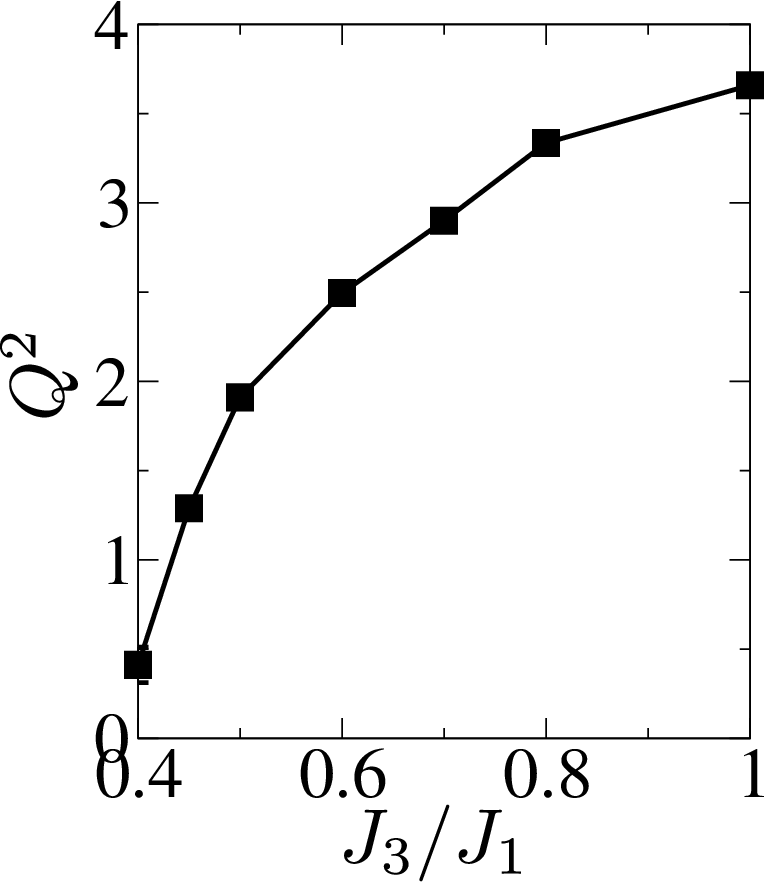
We have performed extensive series expansion calculationsOitmaaBook both in the Néel phase and the spin-spiral phase. Unfortunately the series expansion method is not able to probe properties of the SL phase directly. However, the method allows us to find the range of parameters where the SL exists. In the Néel phase the series starts from the simple Ising antiferomagnetic state. In the spin spiral phase the calculation is more tricky. We first impose a classical diagonal spiral with some wave vector and find the total energy of this state . This includes the classical energy and the quantum corrections calculated by means of series expansions. We perform this calculations for many values of and then find numerically the minimum of . Such procedure gives us the ground state energy and the physical wave vector . Plots of the ground state energy , the spiral vector Q, and the static on-site magnetization M for the XY model are presented in Fig. 1.

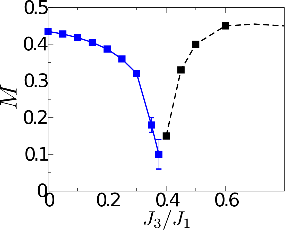
For comparison in Fig. 2 we present the same quantities calculated in Ref. Kharkov2018 for the model.


Note that according to our series calculations the period of the incommensurate spin spiral is quite long. For example implies that r.l.u. So, the period in each direction is lattice spacing. While the series expansion method does not have a problem with this, it can be quite hard to obtain such a long period in a finite cluster calculation. Moreover, the ground state is 4-fold degenerate, . This is on the top of the continuous O(N) degeneracy that results in a well understood rotational tower of quantum states in a finite system Anderson1952; Misguich2002. In the spiral case the continuous group tower must consist of 4-fold split (or degenerate) states due to the degeneracy, and the splitting depends on the geometry of the cluster. It could be nontrivial to disentangle such a spectrum in a finite size cluster numerically.
Concluding this section, the most important qualitative difference between and is the size of the “window” in the parameter space occupied by the SL phase. In the case this is finite interval and in the case it is likely that the interval shrinks to a point. Remarkably the problem of the critical behaviour of the Lifshitz model can be solved exactly. Now we proceed to the solution.
III Zero temperature solution
In the vicinity of the Lifshitz point the spin dynamics is described by an effective nonlinear model with the Lagrangian Ioffe1988
| (2) |
Here is the vector of staggered magnetisation, with , are the spatial gradients , is the transverse magnetic susceptibility. The general form of the “elastic energy” operator assuming that the -field is sufficiently smooth is
| (3) |
The kinematic form of the Lagrangian (2) is dictated by global symmetries of the system. In the case the vector has three components and in the case two components. Hereafter we consider and hence the vector can be parameterised by the single angle
| (4) |
The spin stiffness is the tuning parameter that drives the system across the Lifshitz transition. The spin stiffness is positive in the Néel phase, negative in the spiral phase and vanishes at the Lifshitz point. The 4th order spatial derivative -terms are necessary for stabilisation of the spiral order at negative , and we assume .
The Lagrangian (2) can be rewritten in terms of the angle :
| (5) |
Classically the ground state of this Lagrangian is the collinear Néel state at , and the ground state is the spin spiral at , , where is the wave vector of the spiral. For the spiral wave vector is directed along or , and for the wave vector is directed along the main diagonals.
| (6) | |||||
Parameters of the effective Lagrangians (2),(III) can be expressed in terms of the parameters of the Heisenberg model. These are expansions in powers of spin . For the Heisenberg model on the square lattice in the leading order in the parameters are Ioffe1988; Kharkov2018
| (7) |
The Lagrangian (III) contains quartic in terms. These terms lead to the self-energy of the field . The single loop self-energy diagram is shown in Fig. 3.
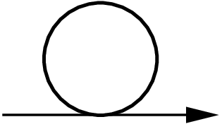
The self-energy has an ultraviolet part that is not singular at and it also has an infrared part singular at . The ultraviolet part just gives subleading corrections in S to equations (III). For example, the quartic terms result in the positive ultraviolet correction to which extends the region of the Neel phase in Fig.1. The Lifshiz point shifts to from the classical Lifshits point that follows from Eqs. (III). It is interesting to note that quantum fluctuations extend the region of the Néel phase, this is the general property of Lifshitz criticality. Kharkov2018 On the other hand in the model quantum fluctuations shrink the region of the Néel phase. The classical critical point is and the quantum critical point is . Sushkov2001 This observation confirms our point that the model does not belong to the Lifshitz class.
The infrared part of the self energy is more interesting, as it influences critical properties, and we discuss this point below. The transverse susceptibility does not have an infrared divergent correction, and in the single loop approximation, Fig. 3, the correction is actually zero. Therefore hereafter we set and hence use dimensionless parameters
| (8) |
The last line defines a dimensionless temperature that we use in the next section.
The values of the coefficients and depend on the specific choice of the lattice model. The special case corresponds to the situation when the ground state energy is degenerate with respect to the direction of . In this degenerate case one has to account for higher order terms in the powers of the spatial gradients in the expansion of the elastic energy . In this work we assume that the system is far away from the degeneracy point, .
III.1 Spin stiffness renormalization
Let us approach the Lifshitz point from the Néel phase, . Quadratic in terms of the Lagrangian (III) result in the following dispersion
| (9) |
where is the momentum. At the Lifshitz point, , the dispersion is quadratic in momentum, and the dynamical critical exponent is ,
| (10) |
To calculate the self-energy Fig. 3 we decouple the nonlinear terms in the Lagrangian (III)
| (11) |
Thus, the self-energy results in a correction to the spin stiffness. First we perform the ultraviolet renormalization. To do so consider the Lifshitz point, . Here the correction is
| (12) |
The integral is convergent in the infrared limit in spite of the quadratic dispersion. Hence, is just a constant that has to be added to the relation (III). We absorb this shift in the definition of . Away from the Lifshitz point in the Néel phase the self-energy leads to a logarithmic renormalization of the spin stiffness, . Similar to (12) we find
| (13) |
For self consistency in the dispersion in this formula we must replace , see Eq.(9). Evaluation of the integral in (13) with logarithmic accuracy is straightforward. This leads to the following equation for the renormalised spin stiffness
| (14) |
Here is the ultraviolet momentum cutoff, is the lattice spacing, and the number is the following angular integral
| (15) |
The logarithmic correction to the spin stiffness can not depend on the sign of , so (14) is valid also for . This point is obvious since the logarithmic correction comes from quantum fluctuations in the momentum range . This range is insensitive to formation of the spin spiral. This implies that in Eqs. (III) one must replace and the correct scaling of the wave vector is
| (16) |
where the constants A and B are given by Eq.(14). So, there is a logarithmic correction to the power scaling of Q. Besides the general scaling arguments one can check the relation by a detailed calculation. To do so we substitute in the Lagrangian (III) and expand it up to cubic terms . A straightforward decoupling procedure leads directly to Eq. (14). The logarithmic correction in Eq. (16) is small. Therefore the deviation of Fig.1b from a straight line is due to the higher powers of that cannot be captured by the field theory.
It is interesting to note that nonlinear terms in the Lagrangian (III) do not renormalize the higher derivative terms . Such corrections can only be generated by subleading terms, e.g. or .
In the spin spiral phase it is convenient to describe excitations in terms of the field . The substitution in the Lagrangian (III) results in the following quadratic form
| (17) |
Hence the effective spin stiffness tensor that determines the spectrum of excitations in the spin spiral phase reads:
| (18) |
Hence the excitation spectrum in the spin spiral phase is
| (19) |
III.2 Spin-spin correlator
From Eq.(9) we conclude that the phase fluctuation in the Néel phase reads
| (20) |
The fluctuation remains finite everywhere except of the point where the integral in (20) is infrared divergent. This confirms the hint given by Fig.1c that the spin liquid is realised only at one point. Everywhere else the long range order is preserved. To calculate the spin-spin correlator in the SL phase we follow the method of Ref.Ardonne2004 The equal time correlator of the -field can be expressed in terms of the correlation function, :
| (21) |
The -field Green’s function reads
| (22) |
Hence
| (23) | |||
Here the angle describes the orientation of the radius vector in the 2D plane . The first term in the square brackets is convergent at large while the second term is logarithmically divergent. Therefore, the first term just provides the lower limit of integration, , for the second one. Hence, at
| (24) |
where
| (25) | |||
Thus the spin-spin correlator at the critical point, , decays algebraically
| (26) |
Interestingly, this correlator decay for the XY-Lifshitz spin liquid is similar to that in the dimer models at the Rokhsar-Kivelson critical point Ardonne2004; Ghaemi2005.
III.3 Static magnetization
The staggered magnetization in the Neel phase, , is
| (27) |
We choose the -axis as the direction of spontaneous symmetry breaking in the Neel phase. The fluctuation of phase is given by Eq.(20). According to Eq.(9) there is a regime crossover at
| (28) |
At the dispersion is quadratic in q, and at the dispersion is linear in q. Therefore, is the infrared cutoff in the logarithmically divergent integral in (20). Hence
| (29) |
This results in the following critical behaviour of the static magnetisation
| (30) |
It is easy to check that the static magnetisation in the spin-spiral phase has the same scaling .
Thus we come to the following conclusions of this section.
(i) The SL is realised only at the critical point, .
(ii) The spin-spin correlator in the SL phase decays algebraically
.
(iii) The static magnetisation away from the SL point scales as
. The critical index is not a universal number, but it depends
on parameters of the system, see Eq.(25). For the model
the critical point is , see Fig. 1c.
Hence using Eq.(III) we estimate .
(iv) Because of the logarithmic correction in Eq.(14)
the critical scaling is not just a power, but there is a logarithmic
dependence.
(v) The incommensurate wave vector scaling in the spin spiral phase also
has a logarithmic correction, Eq.(16).
IV Finite temperature properties
IV.1 Spin stiffness renormalization
In this section we consider the effects of finite temperature T on Lifshitz criticality. We assume that the temperature is much smaller than the energy ultraviolet cutoff, , but it can be larger or comparable with . It is obvious that with these conditions temperature does not influence the ultraviolet renormalization (12). However, the infrared renormalization (13) is changed. The term in the square brackets in (13) should be replaced by a term containing a bosonic occupation number factor , where
| (31) |
Hence Eq.(13) modified for the case of finite reads
| (32) |
This equation is written for the Néel phase. For low temperature, , the last line in Eq.(IV.1) is negligible and we return back to (13). However, for temperature is significant and evaluation of (IV.1) gives
| (33) |
where
| (34) |
An equation similar to (33) was obtained in Ref.Ghaemi2005 for a particular case . Note that Eq. (33) has a positive solution, , for small negative . This means that the stability region of the commensurate fluctuating “Neel” phase at finite temperatures extends towards negative , as shown in the phase diagram in Fig. 4.

IV.2 Magnon lifetime effect
When considering Eq.(33) at very small we will face a serious problem. The equation (33) does not have a solution . Hence the transition line in Fig. 4 between the fluctuating Néel state and the fluctuating spin spiral state is undetermined. To resolve this problem we need to consider perturbative and non-perturbative (topological) fluctuations. In this subsection we consider perturbative fluctuations. Equation (33) is derived in the single loop approximation, see Fig. 3. In this approximation the self-energy does not have an imaginary part. The imaginary part arises due to the double loop diagram shown in Fig. 5.

The four-magnon vertex in Fig.5 is generated by quartic terms in Eq.(III). In what follows we denote by the momentum of the probe magnon, and , , are momenta of magnons from the heat bath. There are three types of the scattering processes contributing to the width: (i) Decay: , (ii) Raman: , (iii) Fusion: We consider the most important Raman process, the corresponding width reads (see e.g. Ref. Scammell2017):
| (35) | |||||
We are interested in the case , hence the dispersion is , . The occupation numbers can be replaced as . Evaluation of the integral in (35) is straightforward, the result is
| (36) |
This estimate is valid if . At very small this condition is violated and hence in the right hand side of (36) we have to replace . This immediately gives the following estimate for at very small
| (37) |
This width results in the effective infrared cutoff in the integration in the last line of Eq.(IV.1). Hence, with account of the width, Eq.(33) is replaced by
| (38) | |||||
The integral in the numerator of this equation has been calculated with logarithmic accuracy, , where is the lifetime infrared cutoff that follows from Eq.(37). However, in the end, the logarithm proved to be not large. Therefore, we must replace it by a constant that we cannot calculate within accuracy of the method. We can only claim that the constant is positive since the integral in the second line of Eq.(IV.1) is positive. The transition line in Fig. 4 between the fluctuating Néel state and the fluctuating spin spiral state is given by the condition , that results in the condition
| (39) |
IV.3 Finite temperature spin-spin correlators
Let us consider the spin-spin correlator at the transition line , see Fig. 4. At a finite temperature Eq.(23) is transformed to
| (40) |
where . The first integral in this equation is infrared logarithmic divergent. As was discussed in the previous subsection the integral has to be regularised by the finite width, . Evaluation of the integrals in (IV.3) is straightforward. At the correlator decays with distance exactly like that in the zero temperature SL, Eq.(26), and at it very quickly decays to zero.
Away from the critical line, , at sufficiently large distances, , the spin-spin correlator decays according to the standard XY-model algebraic law
| (41) |
IV.4 The role of vortices
A single vortex in the XY-model has energy
| (42) |
where is the size of the vortex (size of the sample), and is the energy of the vortex core. Hence at a finite temperature the free energy per vortex reads
| (43) |
The third term in this equation is due to the entropy of the vortex gas . In the usual unfrustrated XY-model (), the core energy . Therefore the core energy does not play a significant role. In the limit the vortex proliferation is energetically favourable () at the temperatures above the BKT temperature . Formally near the Lifshitz point the situation is similar and we can write the following equation for .
| (44) |
In particular at . Obviously Eq.(44) is not consistent with Fig.4. The explanation is that this equation represent a rather formal statement. While at the Lifshitz point the spin stiffness is approaching zero due to frustration, , the core energy remains finite, , see Ref.Kharkov17 According to Eq.(43) in the limit and at vortexes proliferate at any nonzero temperature. This is consistent with Eq.(44). However, to make this point valid the entropy in Eq.(43) must dominate over the core energy, hence the sample size must be sufficiently large, . This can be a huge number, thousands, millions, or billions of lattice spacings that is never achieved in a real sample or in numerical experiments on a finite cluster.
Thus formally mathematically the transition line in Fig. 4 originating from consists of two diverging phase boundary lines that are exponentially close to each other. The intermediate phase between the lines is the deconfined vortex phase. However, in a real sample, say sites, still there is single transition line that at a certain temperature starts to diverge into two BKT lines as it is shown in Fig. 4. The position of the divergence point depends on the sample size dramatically, so the notion of the phase diagram near the divergence point is poorly defined.
To summarise this subsection, at finite system size and at a
sufficiently low temperature the topological excitations (vortices) are
irrelevant near the Lifshitz point. This is because the vortex core energy
remains finite even if the spin stiffness is zero.
Interestingly, in the case (isotropic Heisenberg model) the energy
of the topological excitation, skyrmion, scales proportionally to the spin stiffness.
Therefore, in this case topological excitations are relevant near the Lifshitz point.
V Discussion and conclusion.
We have considered the Lifshitz quantum phase transition problem for the 2D
frustrated XY-model. Here are the conclusions.
(i) We have performed numerical series expansion calculations for
model on the square lattice (). The calculations indicate that
the Lifshitz point behaviour is very different for the
XY- and for the SU(2)-symmetric versions of the model.
(ii) Motivated by the numerics we performed field theory
analysis of the XY-Lifshitz criticality. This analysis results in
the following points.
(iii) The Lifshitz spin liquid phase exists only at the Lifshitz point.
This is different from the SU(2) case where the spin liquid phase occupies a
finite interval in the parameter space.
(iv) At zero temperature we calculate nonuniversal critical exponents in the
Néel and in the spin spiral state and relate them to properties of the spin
liquid.
(v) We also solve the transition problem at a finite temperature,
calculate the critical exponents, and discuss the role of the magnon
lifetime on the finite temperature critical behaviour.
(vi) We show that the topological excitations are irrelevant at low
temperature even near the critical point.
Acknowledgements.
We thank Matthew O’Brien for discussions and Anders Sandvik for important communications. The work has been supported by the Australian Research Council No DP160103630.References
- (1) L. B. Ioffe and A. I. Larkin, J. Mod. Phys. B 2, 203 (1988).
- (2) E. Ardonne, P. Fendley, E. Fradkin, Annals Phys. 310 493 (2004).
- (3) L. Capriotti and S. Sachdev, Phys. Rev. Lett. 93, 257206 (2004).
- (4) E. Fradkin, Field Theories of Condensed Matter Physics 2nd edn (Addison Wesley, 2013).
- (5) L. Balents and O.A. Starykh, Phys. Rev. Lett. 116, 177201 (2016).
- (6) Y. A. Kharkov, J. Oitmaa, O. P. Sushkov, Phys. Rev. B 98, 144420 (2018).
- (7) Y. A. Kharkov, O. P. Sushkov, Phys. Rev. B 98, 155118 (2018).
- (8) Y. A. Kharkov, O. P. Sushkov, arXiv:1901.05587.
- (9) D. S Rokhsar, and S. A. Kivelson, Phys. Rev. Lett. 61, 2376 (1988).
- (10) P. M. Chaikin, and T. C. Lubensky, Principles of Condensed Matter Physics (Cambridge University Press, 1995).
- (11) H. C. Po and Q. Zhou, Nat. Comm. 6 8012 (2015).
- (12) P. Horava, Phys. Rev. D 79, 084008 (2009).
- (13) C. Hoyos, B. S. Kim, Y. Oz, JHEP 03, 029 (2014).
- (14) H. Schenck, V. L. Pokrovsky, and T. Nattermann, Phys. Rev. Lett. 112, 157201 (2014).
- (15) J. Ferrer, Phys. Rev. B 47, 8769 (1993).
- (16) O. P. Sushkov, J. Oitmaa, Zheng Weihong, Phys. Rev. B 63, 104420 (2001).
- (17) L. Capriotti, D. J. Scalapino, and S. R. White, Phys. Rev. Lett. 93, 177004 (2004).
- (18) P. Sindzingre, N. Shannon, and T. Momoi, J. Phys. Conf. Ser. 200, 022058 (2010).
- (19) J. Reuther, P. Wölfle, R. Darradi, W. Brenig, M. Arlego, and J. Richter, Phys. Rev. B 83, 064416 (2011).
- (20) Z. Zhu, D. A. Huse, and S. R. White, Phys. Rev. Lett. 110, 127205 (2013).
- (21) R. F. Bishop, P. H. Y. Li, O. Götze, J. Richter, and C. E. Campbell, Phys. Rev. B 92, 224434 (2015).
- (22) J. Oitmaa, C. Hamer, W. Zheng, Series expansion methods for strongly interacting lattice models, Cambridge University Press (2006).
- (23) P. W. Anderson, Phys. Rev. 86, 694 (1952).
- (24) G. Misguich, C. Lhuillier, M. Mambrini, and P. Sindzingre, Eur. Phys. J. B 26, 167-183 (2002).
- (25) P. Ghaemi, A. Vishwanath, T. Senthil, Phys. Rev. B 72, 024420 (2005).
- (26) H. D. Scammell and O. P. Sushkov, Phys. Rev. B 95, 024420 (2017).
- (27) Y. A. Kharkov, O. P. Sushkov, M. Mostovoy, Phys. Rev. Lett. 119, 207201 (2017).