跳到论文正文
W Papers独立论文阅读器 arXiv:1910.09701 论文正文 计算阅读时间 · 0%
引用这篇论文根据当前论文元数据生成,正式投稿前建议核对。


License: arXiv.org perpetual non-exclusive license
arXiv:1910.09701v2 [stat.ML] 16 Nov 2019

Direct Estimation of Differential Functional Graphical Models

Boxin Zhao Affiliation: Department of Statistics Affiliation: The Unveristy of Chicago Affiliation: Chicago, IL 60637 Email: boxinz@uchicago.edu    Y. Samuel Wang Affiliation: Booth School of Business Affiliation: The Unveristy of Chicago Affiliation: Chicago, IL 60637 Email: swang24@uchicago.edu    Mladen Kolar Affiliation: Booth School of Business Affiliation: The Unveristy of Chicago Affiliation: Chicago, IL 60637 Email: mkolar@chicagobooth.edu
Abstract

We consider the problem of estimating the difference between two functional undirected graphical models with shared structures. In many applications, data are naturally regarded as high-dimensional random function vectors rather than multivariate scalars. For example, electroencephalography (EEG) data are more appropriately treated as functions of time. In these problems, not only can the number of functions measured per sample be large, but each function is itself an infinite dimensional object, making estimation of model parameters challenging. We develop a method that directly estimates the difference of graphs, avoiding separate estimation of each graph, and show it is consistent in certain high-dimensional settings. We illustrate finite sample properties of our method through simulation studies. Finally, we apply our method to EEG data to uncover differences in functional brain connectivity between alcoholics and control subjects.

1 Introduction

Undirected graphical models are widely used to compactly represent pairwise conditional independence in complex systems. Let G={V,E}G=\{V,E\} denote an undirected graph where VV is the set of vertices with |V|=p|V|=p and E⊂V2E\subset V^{2} is the set of edges. For a random vector X=(X1,…,Xp)TX=(X_{1},\dots,X_{p})^{T}, we say that XX satisfies the pairwise Markov property with respect to GG if Xv / ⟂ ⟂Xw|{Xu}u∈V∖{v,w}X_{v}\mathchoice{\mathrel{\hbox to0.0pt{\kern 16.99988pt\kern-5.27776pt$\displaystyle\not$\hss}{\mathchoice{\mathrel{\hbox to0.0pt{ $\displaystyle\perp$ \hss}\mkern 2.0mu{\displaystyle\perp}}}{\mathrel{\hbox to0.0pt{ $\textstyle\perp$ \hss}\mkern 2.0mu{\textstyle\perp}}}{\mathrel{\hbox to0.0pt{ $\scriptstyle\perp$ \hss}\mkern 2.0mu{\scriptstyle\perp}}}{\mathrel{\hbox to0.0pt{ $\scriptscriptstyle\perp$ \hss}\mkern 2.0mu{\scriptscriptstyle\perp}}}}}}{\mathrel{\hbox to0.0pt{\kern 16.99988pt\kern-5.27776pt$\textstyle\not$\hss}{\mathchoice{\mathrel{\hbox to0.0pt{ $\displaystyle\perp$ \hss}\mkern 2.0mu{\displaystyle\perp}}}{\mathrel{\hbox to0.0pt{ $\textstyle\perp$ \hss}\mkern 2.0mu{\textstyle\perp}}}{\mathrel{\hbox to0.0pt{ $\scriptstyle\perp$ \hss}\mkern 2.0mu{\scriptstyle\perp}}}{\mathrel{\hbox to0.0pt{ $\scriptscriptstyle\perp$ \hss}\mkern 2.0mu{\scriptscriptstyle\perp}}}}}}{\mathrel{\hbox to0.0pt{\kern 16.99988pt\kern-4.45831pt$\scriptstyle\not$\hss}{\mathchoice{\mathrel{\hbox to0.0pt{ $\displaystyle\perp$ \hss}\mkern 2.0mu{\displaystyle\perp}}}{\mathrel{\hbox to0.0pt{ $\textstyle\perp$ \hss}\mkern 2.0mu{\textstyle\perp}}}{\mathrel{\hbox to0.0pt{ $\scriptstyle\perp$ \hss}\mkern 2.0mu{\scriptstyle\perp}}}{\mathrel{\hbox to0.0pt{ $\scriptscriptstyle\perp$ \hss}\mkern 2.0mu{\scriptscriptstyle\perp}}}}}}{\mathrel{\hbox to0.0pt{\kern 16.99988pt\kern-3.95834pt$\scriptscriptstyle\not$\hss}{\mathchoice{\mathrel{\hbox to0.0pt{ $\displaystyle\perp$ \hss}\mkern 2.0mu{\displaystyle\perp}}}{\mathrel{\hbox to0.0pt{ $\textstyle\perp$ \hss}\mkern 2.0mu{\textstyle\perp}}}{\mathrel{\hbox to0.0pt{ $\scriptstyle\perp$ \hss}\mkern 2.0mu{\scriptstyle\perp}}}{\mathrel{\hbox to0.0pt{ $\scriptscriptstyle\perp$ \hss}\mkern 2.0mu{\scriptscriptstyle\perp}}}}}}X_{w}|\{X_{u}\}_{u\in V\setminus\{v,w\}} implies {v,w}∈E\{v,w\}\in E. When XX follows a multivariate Gaussian distribution with covariance Σ=Θ−1\Sigma=\Theta^{-1}, then Θv​w≠0\Theta_{vw}\neq 0 implies {v,w}∈E\{v,w\}\in E. Thus, recovering the structure of the undirected graph is equivalent to estimating the support of the precision matrix, Θ\Theta [10, 13, 4, 24, 25].

We consider a setting where we observe two samples XX and YY from (possibly) different distributions, and the primary object of interest is the difference between the conditional dependencies of each population rather than the conditional dependencies in each population. For example, in Section 4.3 we analyze neuroscience data sampled from a control group and a group of alcoholics, and seek to understand how the brain functional connectivity patterns in the alcoholics differ from the control group. Thus, in this paper, the object of interest is the differential graph, GΔ={V,EΔ}G_{\Delta}=\{V,E_{\Delta}\}, which is defined as the difference between the precision matrix of XX, ΘX\Theta^{X} and the precision matrix of YY, ΘY\Theta^{Y}, Δ=ΘX−ΘY\Delta=\Theta^{X}-\Theta^{Y}. When Δv​w≠0\Delta_{vw}\neq 0, it implies {v,w}∈EΔ\{v,w\}\in E_{\Delta}. This type of differential model has been adopted in [30, 22, 3].

In this paper, we are interested in estimating the differential graph in a more complicated setting. Instead of observing vector valued data, we assume the data are actually random vector valued functions (see [5] for a detailed exposition of random functions). Indeed, we aim to estimate the difference between two functional graphical models and the method we propose combines ideas from graphical models for functional data and direct estimation of differential graphs.

Multivariate observations measured across time can be modeled as arising from distinct, but similar distributions [9]. However, in some cases, it may be more natural to assume the data are measurements of an underlying continuous process [31, 18, 11, 28]. [31, 18] treat data as curves distributed according to a multivariate Gaussian process (MGP). [31] shows that Markov properties hold for Gaussian processes, while [18] shows how to consistently estimate underlying conditional independencies.

We adopt the functional data point of view and assume the data are curves distributed according to a MGP. However, we consider two samples from distinct populations with the primary goal of characterizing the difference between the conditional cross-covariance functions of each population. Naively, one could apply the procedure of [18] to each sample, and then directly compare the resulting estimated conditional independence structures. However, this approach would require sparsity in both of the underlying conditional independence graphs and would preclude many practical cases; e.g., neither graph could contain hub-nodes with large degree. We develop a novel procedure that directly learns the difference between the conditional independence structures underlying two MGPs. Under an assumption that the difference is sparse, we can consistently learn the structure of the differential graph, even in the setting where individual graphs are dense and separate estimation would suffer.

Our paper builds on recent literature on graphical models for vector valued data, which suggests that direct estimation of the differences between parameters of underlying distributions may yield better results. [12] considers data arising from pairwise interaction exponential families and propose the Kullback-Leibler Importance Estimation Procedure (KLIEP) to explicitly estimate the ratio of densities. [21] uses KLIEP as a first step to directly estimate the difference between two directed graphs. Alternatively, [30, 26] consider two multivariate Gaussian samples, and directly estimate the difference between the two precision matrices. When the difference is sparse, it can be consistently estimated even in the high-dimensional setting with dense underlying precision matrices. [22] extends this approach to Gaussian copula models.

The rest of the paper is organized as follows. In Section 2 we introduce our method for Functional Differential Graph Estimation (FuDGE). In Section 3 we provide conditions under which FuDGE consistently recovers the true differential graph. Simulations and real data analysis are provided in Section 411 1 The code for this part is on https://github.com/boxinz17/FuDGE. Discussion is provided in Section 5. Appendix contains all the technical proofs and additional simulation results.

We briefly introduce some notation used throughout the rest of the paper. Let |⋅|p|\cdot|_{p} denote vector pp-norm and ∥⋅∥p\|\cdot\|_{p} denote the matrix/operator pp-norm. For example, for a p×pp\times{p} matrix AA with entries aj​ka_{jk}, |A|1=∑j,k|aj​k||A|_{1}=\sum_{j,k}|a_{jk}|, ‖A‖1=max⁡∑jk⁡|aj​k|\|A\|_{1}=\max_{k}\sum_{j}|a_{jk}|, |A|∞=maxj,k⁡|aj​k||A|_{\infty}=\max_{j,k}|a_{jk}|, and ‖A‖∞=max⁡∑kj⁡|aj​k|\|A\|_{\infty}=\max_{j}\sum_{k}|a_{jk}|. Let an≍bna_{n}\asymp{b_{n}} denote that z1≤infn|an/bn|≤supn|an/bn|≤z2z_{1}\leq{\inf_{n}|a_{n}/b_{n}|}\leq{\sup_{n}|a_{n}/b_{n}|}\leq z_{2} for some positive constants z1z_{1} and z2z_{2}. Let λmin​(A)\lambda_{\min}(A) and λmax​(A)\lambda_{\max}(A) denote the minimum and maximum eigenvalues, respectively. For a bivariate function g⁡(s,t)g(s,t), we define the Hilbert-Schmidt norm of g⁡(s,t)g(s,t) (or equivalently, the norm of the integral operator it corresponds to) as ‖g‖HS=∫∫⁡{g⁡(s,t)}2​𝑑s​𝑑t\|g\|_{\text{HS}}=\int\int\{g(s,t)\}^{2}dsdt.

2 Methodology

2.1 Functional differential graphical model

Let Xi​(t)=(Xi​1​(t),…,Xi​p​(t))TX_{i}(t)=(X_{i1}(t),\dots,X_{ip}(t))^{T}, i=1,…,nXi=1,\ldots,n_{X}, and Yi​(t)=(Yi​1​(t),…,Yi​p​(t))TY_{i}(t)=(Y_{i1}(t),\dots,Y_{ip}(t))^{T}, i=1,…,nYi=1,\ldots,n_{Y}, be iid pp-dimensional multivariate Gaussian processes with mean zero and common domain 𝒯\mathcal{T} from two different, but connected population distributions, where 𝒯\mathcal{T} is a closed subset of the real line.22 2 Both Xi​(t)X_{i}(t) and Yi​(t)Y_{i}(t) are indexed by ii, but they are not paired observations and are completely independent. Also, we assume mean zero and a common domain 𝒯\mathcal{T} to simplify the notation, but the methodology and theory generalize to non-zero means and different time domains 𝒯X\mathcal{T}_{X} and 𝒯Y\mathcal{T}_{Y} when fixing some bijection 𝒯X↦𝒯Y\mathcal{T}_{X}\mapsto\mathcal{T}_{Y}. Also, assume that for j=1,…,pj=1,\ldots,p, Xi​j​(t)X_{ij}(t) and Yi​j​(t)Y_{ij}(t) are random elements of a separable Hilbert space ℍ\mathbb{H}. For brevity, we will generally only explicitly define notation for Xi​(t)X_{i}(t); however, the reader should note that all notations for Yi​(t)Y_{i}(t) are defined analogously.

Following [18], we define the conditional cross-covariance function for Xi​(t)X_{i}(t) as

Cj​lX​(s,t)=Cov⁡(Xi​j​(s),Xi​l​(t)∣{Xi​k​(⋅)}k≠j,l).{}C^{X}_{jl}(s,t)\;=\;\mathrm{Cov}\left(X_{ij}(s),X_{il}(t)\,\mid\,\{X_{ik}(\cdot)\}_{k\neq j,l}\right). (2.1)

If Cj​lX​(s,t)=0C^{X}_{jl}(s,t)=0 for all s,t∈𝒯s,t\in\mathcal{T}, then the random functions Xi​j​(t)X_{ij}(t) and Xi​l​(t)X_{il}(t) are conditionally independent given the other random functions. The graph GX={V,EX}G_{X}=\{V,E_{X}\} represents the pairwise Markov properties of Xi​(t)X_{i}(t) if

EX={(j,l)∈V2:j≠l​ and ​∃{s,t}∈𝒯2​ such that ​Cj​lX​(s,t)≠ 0}.E_{X}\;=\;\{(j,l)\in V^{2}:\;j\neq l\;\text{ and }\;\exists\{s,t\}\in\mathcal{T}^{2}\,\text{ such that }\,C^{X}_{jl}(s,t)\,\neq\,0\}. (2.2)

In this paper, the object of interest is CΔ​(s,t)C^{\Delta}(s,t) where Cj​lΔ​(s,t)=Cj​lX​(s,t)−Cj​lY​(s,t)C^{\Delta}_{jl}(s,t)=\ C^{X}_{jl}(s,t)-C^{Y}_{jl}(s,t). We define the differential graph to be GΔ={V,EΔ}G_{\Delta}=\{V,E_{\Delta}\}, where

EΔ={(j,l)∈V2:j≠l​ and ​‖Cj​lΔ‖H​S≠ 0}.{}E_{\Delta}\;=\;\{(j,l)\in{V^{2}}:\;j\neq l\;\text{ and }\;\|C^{\Delta}_{jl}\|_{HS}\,\neq\,0\}. (2.3)

Again, we include an edge between jj and ll, if the conditional dependence between Xi​j​(t)X_{ij}(t) and Xi​l​(t)X_{il}(t) given all the other curves differs from that of Yi​j​(t)Y_{ij}(t) and Yi​l​(t)Y_{il}(t) given all the other curves.

2.2 Functional principal component analysis

Since Xi​(t)X_{i}(t) and Yi​(t)Y_{i}(t) are infinite dimensional objects, for practical estimation, we reduce the dimensionality using functional principal component analysis (FPCA). Similar to the way principal component analysis provides an L2L_{2} optimal lower dimensional representation of vector valued data, FPCA provides an L2L_{2} optimal finite dimensional representation of functional data. As in [18], for simplicity of exposition, we assume that we fully observe the functions Xi​(t)X_{i}(t) and Yi​(t)Y_{i}(t). However, FPCA can also be applied to both densely and sparsely observed functional data, as well as data containing measurement errors. Such an extension is straightforward, cf. [23] and [20] for a recent overview. Let Kj​jX​(t,s)=Cov⁡(Xi​j​(t),Xi​j​(s))K^{X}_{jj}(t,s)=\mathrm{Cov}(X_{ij}(t),X_{ij}(s)) denote the covariance function for Xi​jX_{ij}. Then, there exists orthonormal eigenfunctions and eigenvalues {ϕj​k​(t),λj​kX}k∈ℕ\{\phi_{jk}(t),\lambda^{X}_{jk}\}_{k\in\mathbb{N}} such that for all k∈ℕk\in\mathbb{N} [5]:

∫𝒯Kj​jX​(s,t)​ϕj​kX​(t)​𝑑t=λj​kX​ϕj​kX​(s).\int_{\mathcal{T}}K^{X}_{jj}(s,t)\phi_{jk}^{X}(t)dt=\lambda_{jk}^{X}\phi_{jk}^{X}(s). (2.4)

Without loss of generality, assume λj​1X≥λj​2X≥⋯≥0\lambda^{X}_{j1}\geq\lambda^{X}_{j2}\geq\dots\geq 0. By the Karhunen-Loève expansion [5, Theorem 7.3.5], Xi​j​(t)X_{ij}(t) can be expressed as Xi​j​(t)=∑k=1∞ai​j​kX​ϕj​kX​(t)X_{ij}(t)=\sum_{k=1}^{\infty}a^{X}_{ijk}\phi^{X}_{jk}(t) where the principal component scores satisfy ai​j​kX=∫𝒯Xi​j​(t)​ϕj​kX​(t)​𝑑ta^{X}_{ijk}=\int_{\mathcal{T}}X_{ij}(t)\phi^{X}_{jk}(t)dt and ai​j​kX∼N⁡(0,λj​kX)a^{X}_{ijk}\sim N(0,\lambda_{jk}^{X}) with E⁡(ai​j​kX​ai​j​lX)=0E(a^{X}_{ijk}a^{X}_{ijl})=0 if k≠lk\neq l. Because the eigenfunctions are orthonormal, the L2L_{2} projection of Xi​jX_{ij} onto the span of the first MM eigenfunctions is

Xi​jM​(t)=∑k=1Mai​j​kX​ϕj​kX​(t).X^{M}_{ij}(t)=\sum_{k=1}^{M}a^{X}_{ijk}\phi^{X}_{jk}(t). (2.5)

Functional PCA constructs estimators ϕ^j​kX​(t)\hat{\phi}^{X}_{jk}(t) and a^i​j​kX\hat{a}^{X}_{ijk} through the following procedure. First, we form an empirical estimate of the covariance function:

K^j​jX​(s,t)=1nX​∑i=1nX(Xi​j​(s)−Xj¯​(s))​(Xi​j​(t)−Xj¯​(t)),\hat{K}^{X}_{jj}(s,t)=\frac{1}{n_{X}}\sum^{n_{X}}_{i=1}(X_{ij}(s)-\bar{X_{j}}(s))(X_{ij}(t)-\bar{X_{j}}(t)),

where Xj¯​(t)=nX−1​∑i=1nXXi​j​(t)\bar{X_{j}}(t)=n_{X}^{-1}\sum^{n_{X}}_{i=1}X_{ij}(t). An eigen-decomposition of K^j​jX​(s,t)\hat{K}^{X}_{jj}(s,t) then directly provides the estimates λ^j​kX\hat{\lambda}^{X}_{jk} and ϕ^j​kX\hat{\phi}^{X}_{jk} which allow for computation of a^i​j​kX=∫𝒯Xi​j​(t)​ϕ^j​kX​(t)​𝑑t\hat{a}^{X}_{ijk}=\int_{\mathcal{T}}X_{ij}(t)\hat{\phi}^{X}_{jk}(t)dt. Let ai​jX,M=(ai​j​1X,…,ai​j​MX)T∈ℝMa^{X,M}_{ij}=(a^{X}_{ij1},\dots,a^{X}_{ijM})^{T}\in{\mathbb{R}^{M}} and aiX,M=((ai​1X,M)T,…,(ai​pX,M)T)T∈ℝp​Ma^{X,M}_{i}=((a^{X,M}_{i1})^{T},\ldots,(a^{X,M}_{ip})^{T})^{T}\in{\mathbb{R}^{pM}} with corresponding estimates a^i​jX,M\hat{a}^{X,M}_{ij} and a^iX,M\hat{a}^{X,M}_{i}. Since XiM​(t)X^{M}_{i}(t) are p-dimensional MGP, aiX,Ma^{X,M}_{i} will have a multivariate Gaussian distribution with p​M×p​MpM\times pM covariance matrix which we denote as ΣX,M=(ΘX,M)−1\Sigma^{X,M}=(\Theta^{X,M})^{-1}. In practice, MM can be selected by cross validation as in [18].

For (j,l)∈V2(j,l)\in{V^{2}}, let Θj​lX,M\Theta^{X,M}_{jl} be the M×MM\times{M} matrix corresponding to (j,l)(j,l)th submatrix of ΘX,M\Theta^{X,M}. Let ΔM=ΘX,M−ΘY,M\Delta^{M}=\Theta^{X,M}-\Theta^{Y,M} be the difference between the precision matrices of the first MM principal component scores where Δj​lM\Delta^{M}_{jl} denotes the (j,l)(j,l)th submatrix of ΔM\Delta^{M}. In addition, let

EΔM≔{(j,l)∈V2:‖Δj​lM‖F≠0},{}E_{\Delta^{M}}\coloneqq\{(j,l)\in{V^{2}}:\|\Delta^{M}_{jl}\|_{F}\neq{0}\}, (2.6)

denote the set of non-zero blocks of the difference matrix ΔM\Delta^{M}. In general EΔM≠EΔE_{\Delta^{M}}\neq E_{\Delta}; however, we will see that for certain MM, by constructing a suitable estimator of ΔM\Delta^{M} we can still recover EΔE_{\Delta}.

2.3 Functional differential graph estimation

We now describe our method, FuDGE, for functional differential graph estimation. Let SX,MS^{X,M} and SY,MS^{Y,M} denote the sample covariances of a^iX,M\hat{a}^{X,M}_{i} and a^iY,M\hat{a}^{Y,M}_{i}. To estimate ΔM\Delta^{M}, we solve the following problem with the group lasso penalty, which promotes blockwise sparsity in Δ^M\hat{\Delta}^{M} [27]:

Δ^M∈arg​minΔ∈ℝpM×pM⁡L​(Δ)+λn​∑{i,j}∈V2‖Δij‖F,\hat{\Delta}^{M}\in\argmin_{\Delta\in{\mathbb{R}^{pM\times pM}}}L(\Delta)+\lambda_{n}\sum_{\{i,j\}\in V^{2}}\|\Delta_{ij}\|_{F}, (2.7)

where L⁡(Δ)=tr⁡[12​SY,M​ΔT​SX,M​Δ−ΔT​(SY,M−SX,M)]L(\Delta)=\mathrm{tr}\left[\frac{1}{2}S^{Y,M}\Delta^{T}{S^{X,M}}\Delta-\Delta^{T}\left(S^{Y,M}-S^{X,M}\right)\right]. Note that although the true ΔM\Delta^{M} is symmetric, we do not enforce symmetry in Δ^M\hat{\Delta}^{M}.

The design of the loss function L⁡(Δ)L(\Delta) in equation (2.7) is based on [15], where in order to construct a consistent M-estimator, we want the true parameter value ΔM\Delta^{M} to minimize the population loss 𝔼⁡[L⁡(Δ)]\mathbb{E}\left[L(\Delta)\right]. For a differentiable and convex loss function, this is equivalent to selecting LL such that 𝔼⁡[∇L​(ΔM)]=0\mathbb{E}\left[\nabla L(\Delta^{M})\right]=0. Since ΔM=(ΣX,M)−1−(ΣY,M)−1\Delta^{M}=\left(\Sigma^{X,M}\right)^{-1}-\left(\Sigma^{Y,M}\right)^{-1}, it satisfies ΣX,M​ΔM​ΣY,M−(ΣY,M−ΣX,M)=0\Sigma^{X,M}\Delta^{M}\Sigma^{Y,M}-(\Sigma^{Y,M}-\Sigma^{X,M})=0. By this observation, a choice for ∇L​(Δ)\nabla L(\Delta) is

∇L​(ΔM)=SX,M​ΔM​SY,M−(SY,M−SX,M),\nabla{L(\Delta^{M})}=S^{X,M}\Delta^{M}{S^{Y,M}}-\left(S^{Y,M}-S^{X,M}\right), (2.8)

for which 𝔼⁡[∇L​(ΔM)]=ΣX,M​ΔM​ΣY,M−(ΣY,M−ΣX,M)=0\mathbb{E}\left[\nabla L(\Delta^{M})\right]=\Sigma^{X,M}\Delta^{M}\Sigma^{Y,M}-(\Sigma^{Y,M}-\Sigma^{X,M})=0. Using properties of the differential of the trace function, this choice of ∇L​(Δ)\nabla L(\Delta) yields L⁡(Δ)L(\Delta) in (2.7). The chosen loss is quadratic (see (B.10) in supplement) and leads to an efficient algorithm. Such loss has been used in [22, 26, 14] and [30].

Finally, to form E^Δ\hat{E}_{\Delta}, we threshold Δ^M\hat{\Delta}^{M} by ϵn>0\epsilon_{n}>0 so that:

E^Δ={(j,l)∈V2:‖Δ^j​lM‖F>ϵn​or​‖Δ^l​jM‖F>ϵn}.{}\hat{E}_{\Delta}=\{(j,l)\in{V^{2}}:\|\hat{\Delta}^{M}_{jl}\|_{F}>\epsilon_{n}\;\text{or}\;\|\hat{\Delta}^{M}_{lj}\|_{F}>\epsilon_{n}\}. (2.9)

2.4 Optimization algorithm for FuDGE

Algorithm 1 Functional differential graph estimation
0:  SX,M,SY,M,λn,ηS^{X,M},S^{Y,M},\lambda_{n},\eta.
0:  Δ^M\hat{\Delta}^{M}.
 Initialize Δ(0)=0p​M\Delta^{(0)}=0_{pM}.
 repeat
  A=Δ−η∇L(Δ)=Δ−η[SX(M)ΔSY(M)−(SY(M)−SX(M))]A=\Delta-\eta\nabla L(\Delta)=\Delta-\eta\left[S^{(M)}_{X}\Delta S^{(M)}_{Y}-(S^{(M)}_{Y}-S^{(M)}_{X})\right]
  for 1≤i,j≤p1\leq{i,j}\leq{p} do
   Δj​l←(‖Aj​l‖F−λn​η‖Aj​l‖F)+⋅Aj​l\Delta_{jl}\leftarrow\left(\frac{\|A_{jl}\|_{F}-\lambda_{n}\eta}{\|A_{jl}\|_{F}}\right)_{+}\cdot A_{jl}
  end for
 until Converge

The optimization problem (2.7) can be solved by a proximal gradient method [17], summarized in Algorithm 1. Specifically, in each iteration step, we update the current value of Δ\Delta, denoted as Δold\Delta^{\text{old}}, by solving the following problem:

Δnew=arg​minΔ(12‖Δ−(Δold−η∇L(Δold))‖F2+η⋅λn∑j,l=1p∥Δjl∥F),{}\Delta^{\text{new}}=\argmin_{\Delta}\left(\frac{1}{2}\left\|\Delta-\left(\Delta^{\text{old}}-\eta\nabla L\left(\Delta^{\text{old}}\right)\right)\right\|_{F}^{2}+\eta\cdot\lambda_{n}\sum^{p}_{j,l=1}\|\Delta_{jl}\|_{F}\right), (2.10)

where ∇L​(Δ)\nabla L(\Delta) is defined in (2.8) and η\eta is a user specified step size. Note that ∇L​(Δ)\nabla L(\Delta) is Lipschitz continuous with the Lipschitz constant OPEN‖SY,M⊗SX,M‖2≤(λmax​(SY,M)​λmax​(SX,M)))1/2\|S^{Y,M}\otimes S^{X,M}\|_{2}\leq\left(\lambda_{\max}(S^{Y,M})\lambda_{\max}(S^{X,M})\right))^{1/2}. Thus, for any η\eta such that 0<η≤λmaxS0<\eta\leq\sqrt{\lambda^{S}_{\max}}, the proximal gradient method is guaranteed to converge [1], where λmaxS=λmax​(SY,M)​λmax​(SX,M)\lambda^{S}_{\max}=\lambda_{\max}(S^{Y,M})\lambda_{\max}(S^{X,M}) is the largest eigenvalue of SX,M⊗SY,MS^{X,M}\otimes S^{Y,M}.

The update in (2.10) has a closed-form solution:

Δj​lnew=[(‖Aj​lold‖F−λn​η)/‖Aj​lold‖F]+⋅Aj​lold,1≤j,l≤p,{}\Delta^{\text{new}}_{jl}=\left[\left(\|A^{\text{old}}_{jl}\|_{F}-\lambda_{n}\eta\right)/\|A^{\text{old}}_{jl}\|_{F}\right]_{+}\cdot A^{\text{old}}_{jl},\hskip 20.00003pt1\leq{j,l}\leq{p}, (2.11)

where Aold=Δold−η∇L(Δold)A^{\text{old}}=\Delta^{\text{old}}-\eta\nabla L(\Delta^{\text{old}}) and x+=max⁡{0,x},x∈ℝx_{+}=\max\{0,x\},x\in{\mathbb{R}} represents the positive part of xx. Detailed derivations are given in the appendix.

After performing FPCA, the proximal gradient descent method converges in O⁡(λmaxS/tol)O\left(\lambda^{S}_{\max}/\text{tol}\right) iterations, where tol is error tolerance, each iteration takes O⁡((p​M)3)O((pM)^{3}) operations. See [19] for convergence analysis of proximal gradient descent algorithm.

3 Theoretical properties

In this section, we present theoretical properties of the proposed method. Again, we state assumptions explicitly for Xi​(t)X_{i}(t), but also require the same conditions on Yi​(t)Y_{i}(t).

Assumption 3.1.

Recall that λj​kX\lambda_{jk}^{X} and ϕj​kX​(t)\phi^{X}_{jk}(t) are the the eigenvalues and eigenfunctions of Kj​jX​(t)K^{X}_{jj}(t), the covariance function for Xi​j​(t)X_{ij}(t), and λj​kX≥λj​k′X\lambda^{X}_{jk}\geq\lambda^{X}_{jk^{\prime}} for all k′>kk^{\prime}>k.

  1. (i)

    Assume max⁡∑k=1∞j∈V⁡λj​kX<∞\max_{j\in{V}}\sum_{k=1}^{\infty}\lambda^{X}_{jk}<\infty and there exists some constant βX>1\beta_{X}>1 such that for each k∈ℕk\in\mathbb{N}, λj​kX≍k−βX\lambda^{X}_{jk}\asymp{k^{-\beta_{X}}} and dj​kX​λj​kX=O⁡(k)d^{X}_{jk}\lambda^{X}_{jk}=O(k) uniformly in j∈Vj\in{V}, where dj​kX=2​2​max⁡{(λj⁡(k−1)X−λj​kX)−1,(λj​kX−λj⁡(k+1)X)−1}d^{X}_{jk}=2\sqrt{2}\max\left\{\left(\lambda^{X}_{j(k-1)}-\lambda^{X}_{jk}\right)^{-1},\left(\lambda^{X}_{jk}-\lambda^{X}_{j(k+1)}\right)^{-1}\right\}.

  2. (ii)

    Assume for all k∈ℕk\in\mathbb{N}, ϕj​kX​(t)\phi^{X}_{jk}(t)’s are continuous on the compact set 𝒯\mathcal{T} and satisfy maxj∈Vsups∈𝒯supk≥1|ϕj​kX(s)|=O(1)\max_{j\in{V}}\sup_{s\in{\mathcal{T}}}\sup_{k\geq{1}}|\phi^{X}_{jk}(s)|=O(1).

The parameter βX\beta_{X} controls the decay rate of the eigenvalues and dj​kX​λj​kX=O⁡(k)d^{X}_{jk}\lambda^{X}_{jk}=O(k) controls the decay rate of eigen-gaps (see [2] for more details).

To recover the exact functional differential graph structure, we need further assumptions on the difference operator CΔ={Cj​lX​(s,t)−Cj​lY​(s,t)}j,l∈VC^{\Delta}=\{C^{X}_{jl}(s,t)-C^{Y}_{jl}(s,t)\}_{j,l\in V}. Let ν=ν⁡(M)=max(j,l)∈V2⁡|‖Cj​lΔ‖HS−‖Δj​lM‖F|\nu=\nu(M)=\max_{(j,l)\in V^{2}}\left|\|C^{\Delta}_{jl}\|_{\text{HS}}-\|\Delta^{M}_{jl}\|_{F}\right|, and let τ=min(j,l)∈EΔ⁡‖Cj​lΔ‖HS\tau=\min_{(j,l)\in E_{\Delta}}\|C^{\Delta}_{jl}\|_{\text{HS}}, where τ>0\tau>0 by the definition in (2.3). Roughly speaking, ν⁡(M)\nu(M) measures the bias due to using an MM-dimensional approximation, and τ\tau measures the strength of signal in the differential graph. A smaller τ\tau implies that the graph is harder to recover, and in Theorem 3.1, we require the bias to be small compared to the signal.

Assumption 3.2.

Assume that limM→∞ν⁡(M)=0\lim_{M\rightarrow\infty}\nu(M)=0.

We also require Assumption 3.3 which assumes sparsity in EΔE_{\Delta}. Again, this does not preclude the case where EXE_{X} and EYE_{Y} are dense, as long as the difference between the two graphs is sparse. This assumption is common in the scalar setting; e.g., Condition 1 in [30].

Assumption 3.3.

There are ss edges in the differential graph; i.e., |EΔ|=s|E_{\Delta}|=s.

Before we give conditions for recovering the differential graph with high probability, we first introduce some additional notation. Let n=min⁡{nX,nY}n=\min\{n_{X},n_{Y}\}, σmax=max⁡{|ΣX,M|∞,|ΣY,M|∞}\sigma_{\max}=\max\{|\Sigma^{X,M}|_{\infty},|\Sigma^{Y,M}|_{\infty}\}, β=min⁡{βX,βY}\beta=\min\{\beta_{X},\beta_{Y}\}, and λmin∗=λmin​(ΣX,M)×λmin​(ΣY,M)\lambda^{*}_{\min}=\lambda_{\min}\left(\Sigma^{X,M}\right)\times\lambda_{\min}\left(\Sigma^{Y,M}\right). Denote

δ=M1+β​2​(log⁡p+log⁡M+log⁡n)/n\delta\;=\;M^{1+\beta}\sqrt{2\left(\log{p}+\log{M}+\log{n}\right)/n} (3.1)

and

Γ=9​λn2​sκℒ2+2​λnκℒ​(ωℒ2+2​p2​ν),\Gamma\;=\;\frac{9\lambda^{2}_{n}s}{\kappa^{2}_{\mathcal{L}}}+\frac{2\lambda_{n}}{\kappa_{\mathcal{L}}}(\omega^{2}_{\mathcal{L}}+2p^{2}\nu), (3.2)

where

λn\displaystyle\lambda_{n} = 2​M​[(δ2+2​δ​σm​a​x)​|ΔM|1+2​δ],\displaystyle=\;2M\left[\left(\delta^{2}+2\delta\sigma_{max}\right)\left|\Delta^{M}\right|_{1}+2\delta\right], (3.3)
κℒ\displaystyle\kappa_{\mathcal{L}} =(1/2)​λmin∗−8​M2​s​(δ2+2​δ​σmax), and\displaystyle=\;(1/2)\lambda^{*}_{\min}-8M^{2}s\left(\delta^{2}+2\delta\sigma_{\max}\right),\text{ and }
ωℒ\displaystyle\omega_{\mathcal{L}} = 4​M​p2​ν​δ2+2​δ​σmax.\displaystyle=\;4Mp^{2}\nu\sqrt{\delta^{2}+2\delta\sigma_{\max}}.

Note that Γ\Gamma implicitly depends on nn through λn\lambda_{n}, κℒ\kappa_{\mathcal{L}}, ωℒ\omega_{\mathcal{L}} and δ\delta.

Theoreom 3.1.

There exist positive constants c1c_{1} and c2c_{2}, such that for nn and MM large enough to simultaneously satisfy

0\displaystyle 0 <Γ<(1/2)​τ−ν⁡(M)​ and\displaystyle<\Gamma<(1/2)\tau-\nu(M)\text{ and } (3.4)
δ\displaystyle\delta <min⁡{(1/4)​(λmin∗+16​M2​s​(σmax)2)/(M2​s)−σmax,c13/2},\displaystyle<\min\left\{(1/4)\sqrt{\left(\lambda^{*}_{\min}+16M^{2}s(\sigma_{\max})^{2}\right)/\left(M^{2}s\right)}-\sigma_{\max},\;c_{1}^{3/2}\right\},

setting ϵn∈(Γ+ν⁡(M),τ−(Γ+ν⁡(M)))\epsilon_{n}\in(\Gamma+\nu(M),\tau-(\Gamma+\nu(M))) ensures that

P⁡(E^Δ=EΔ)≥1−2​c2/n2.P\left(\hat{E}_{\Delta}=E_{\Delta}\right)\geq 1-2c_{2}/n^{2}.

[18] assumed for some finite MM, for all j∈Vj\in{V}, λj​m′X=0\lambda^{X}_{jm^{\prime}}=0 for all m′>Mm^{\prime}>M. Under this assumption, Xi​j​(t)=Xi​jM​(t)X_{ij}(t)=X^{M}_{ij}(t), and EXE_{X} will correspond exactly to (j,l)∈V2(j,l)\in{V^{2}} such that ‖Θj​lX,M‖F≠0\|\Theta^{X,M}_{jl}\|_{F}\neq{0} [18, Lemma 1]. If the same eigenvalue condition holds for Yi​(t)Y_{i}(t), then in our setting EΔ=EΔME_{\Delta}=E_{\Delta^{M}}. When this holds and we can fix MM, we obtain consistency even in the high-dimensional setting since ν=0\nu=0 and min⁡{s​log⁡(p​n)​|ΔM|12/n,s​log⁡(p​n)/n}→0\min\{s\log(pn)|\Delta^{M}|_{1}^{2}/n,s\sqrt{\log(pn)/n}\}\rightarrow 0 implies consistent estimation. However, even with an infinite number of positive eigenvalues, high-dimensional consistency is still possible for quickly decaying ν\nu; e.g, if ν=o⁡(p−2​M−1)\nu=o(p^{-2}M^{-1}) the same rate is achievable as when v⁡(M)=0v(M)=0.

4 Experiments

4.1 Simulation study

In this section, we demonstrate properties of our method through simulations. In each setting, we generate nX×pn_{X}\times p functional variables from graph GXG_{X} via Xi​j​(t)=b​(t)T​δi​jXX_{ij}(t)=b(t)^{T}\delta^{X}_{ij}, where b⁡(t)b(t) is a five dimensional basis with disjoint support over [0,1][0,1] with

bk​(t)={cos⁡(10​π​(x−(2​k−1)/10))+1(k−1)/5≤x<k/5;0otherwise,k=1,…,5.b_{k}(t)=\left\{\begin{array}[]{ll}\cos\left(10\pi\left(x-(2k-1)/10\right)\right)+1&(k-1)/5\leq{x}<k/5;\\ 0&\text{otherwise},\end{array}\right.\hskip 20.00003ptk=1,\ldots,5.

δiX=((δi​1X)T,⋯,(δi​pX)T)T∈ℝ5​p\delta^{X}_{i}=((\delta^{X}_{i1})^{T},\cdots,(\delta^{X}_{ip})^{T})^{T}\in{\mathbb{R}^{5p}} follows a multivariate Gaussian distribution with precision matrix ΩX\Omega^{X}. Yi​j​(t)Y_{ij}(t) was generated in a similar way with precision matrix ΩY\Omega^{Y}. We consider three models with different graph structures, and for each model, data are generated with nX=nY=100n_{X}=n_{Y}=100 and p=30,60,90,120p=30,60,90,120. We repeat this 30 times for each pp and model setting.

Refer to caption
Figure 1: Average ROC curves across 30 simulations. Different columns correspond to different models, different rows correspond to different dimensions.

Model 1: This model is similar to the setting considered in [30], but modified to the functional case. We generate support of ΩX\Omega^{X} according to a graph with p⁡(p−1)/10p(p-1)/10 edges and a power-law degree distribution with an expected power parameter of 2. Although the graph is sparse with only 20% of all possible edges present, the power-law structure mimics certain real-world graphs [16] by creating hub nodes with large degree. For each nonzero block, Ωj​lX=δ′​I5\Omega^{X}_{jl}=\delta^{\prime}I_{5}, where δ′\delta^{\prime} is sampled uniformly from ±[0.2,0.5]\pm[0.2,0.5]. To ensure positive definiteness, we further scale each off-diagonal block by 1/2,1/3,1/4,1/51/2,1/3,1/4,1/5 for p=30,60,90,120p=30,60,90,120 respectively. Each diagonal element of ΩX\Omega^{X} is set to 11 and the matrix is symmetrized by averaging it with its transpose. To get ΩY\Omega^{Y}, we first select the largest hub nodes in GXG_{X} (i.e., the nodes with largest degree), and for each hub node we select the top (by magnitude) 20% of edges. For each selected edge, we set Ωj​lY=Ωj​lX+W\Omega^{Y}_{jl}=\Omega^{X}_{jl}+W where Wk​m=0W_{km}=0 for |k−m|≤2|k-m|\leq{2}, and Wk​m=cW_{km}=c otherwise, where cc is generated in the same way as δ′\delta^{\prime}. For all other blocks, Ωj​lY=Ωj​lX\Omega^{Y}_{jl}=\Omega^{X}_{jl}.

Model 2: We first generate a tridiagonal block matrix ΩX∗\Omega^{*}_{X} with ΩX,j​j∗=I5\Omega^{*}_{X,jj}=I_{5}, ΩX,j,j+1∗=ΩX,j+1,j∗=0.6​I5\Omega^{*}_{X,j,j+1}=\Omega^{*}_{X,j+1,j}=0.6I_{5}, and ΩX,j,j+2∗=ΩX,j+2,j∗=0.4​I5\Omega^{*}_{X,j,j+2}=\Omega^{*}_{X,j+2,j}=0.4I_{5} for j=1,…,pj=1,\ldots,p. All other blocks are set to 0. We then set ΩY,j,j+3∗=ΩY,j+3,j∗=W\Omega^{*}_{Y,j,j+3}=\Omega^{*}_{Y,j+3,j}=W for j=1,2,3,4j=1,2,3,4, and let ΩY,j​l∗=ΩX,j​l∗\Omega^{*}_{Y,jl}=\Omega^{*}_{X,jl} for all other blocks. Thus, we form GYG_{Y} by adding four edges to GXG_{X}. We let Wk​m=0W_{km}=0 when |k−m|≤1|k-m|\leq{1}, and Wk​m=cW_{km}=c otherwise, with c=1/10c=1/10 for p=30p=30, c=1/15c=1/15 for p=60p=60, c=1/20c=1/20 for p=90p=90, and c=1/25c=1/25 for p=120p=120. Finally, we set ΩX=ΩX∗+δ​I\Omega^{X}=\Omega^{*}_{X}+\delta I, ΩY=ΩY∗+δ​I\Omega^{Y}=\Omega^{*}_{Y}+\delta I, where δ=max⁡{|min⁡(λmin​(ΩX∗),0)|,|min⁡(λmin​(ΩY∗),0)|}\delta=\max\left\{|\min(\lambda_{\min}(\Omega^{*}_{X}),0)|,|\min(\lambda_{\min}(\Omega^{*}_{Y}),0)|\right\}.

Model 3: We generate ΩX∗\Omega^{*}_{X} according to an Erdös-Rényi graph. We first set ΩX,j​j∗=I5\Omega^{*}_{X,jj}=I_{5}. With probability .8.8, we set ΩX,j​l∗=ΩX,l​j∗=0.1​I5\Omega^{*}_{X,jl}=\Omega^{*}_{X,lj}=0.1I_{5}, and set it to 00 otherwise. Thus, we expect 80% of all possible edges to be present. Then, we form GYG_{Y} by randomly adding ss new edges to GXG_{X}, where s=3s=3 for p=30p=30, s=4s=4 for p=60p=60, s=5s=5 for p=90p=90, and s=6s=6 for p=120p=120. We set each corresponding block ΩY,j​l∗=W\Omega^{*}_{Y,jl}=W, where Wk​m=0W_{km}=0 when |k−m|≤1|k-m|\leq{1} and Wk​m=cW_{km}=c otherwise. We let c=2/5c=2/5 for p=30p=30, c=4/15c=4/15 for p=60p=60, c=1/5c=1/5 for p=90p=90, and c=4/25c=4/25 for p=120p=120. Finally, we set ΩX=ΩX∗+δ​I\Omega^{X}=\Omega^{*}_{X}+\delta I, ΩY=ΩY∗+δ​I\Omega^{Y}=\Omega^{*}_{Y}+\delta I, where δ=max⁡{|min⁡(λmin​(ΩX∗),0)|,|min⁡(λmin​(ΩY∗),0)|}\delta=\max\left\{|\min(\lambda_{\min}(\Omega^{*}_{X}),0)|,|\min(\lambda_{\min}(\Omega^{*}_{Y}),0)|\right\}.

Although the theory assumes fully observed functional data, in order to mimic a realistic setting, we use noisy observations at discrete time points, such that the actual data corresponding to Xi​jX_{ij} are

hi​j​kX=Xi​j​(tk)+ei​j​k,ei​j​k∼N⁡(0,0.52),h^{X}_{ijk}=X_{ij}(t_{k})+e_{ijk},\hskip 10.00002pte_{ijk}\sim N(0,0.5^{2}),

for 200200 evenly spaced time points 0=t1≤⋯≤t200=10=t_{1}\leq\cdots\leq t_{200}=1. hi​j​kYh^{Y}_{ijk} are obtained in a similar way. For each observation, we first estimate a function by fitting an LL-dimensional B-spline basis. We then use these estimated functions for FPCA and our direct estimation procedure. Both MM and LL are chosen by 5-fold cross-validation as discussed in [18]. Since ϵn\epsilon_{n} in (2.9) is usually very small in practice, we simply let E^Δ={(j,l)∈V2:‖Δ^j​lM‖F+‖Δ^l​jM‖F>0}\hat{E}_{\Delta}=\{(j,l)\in{V^{2}}:\;\|\hat{\Delta}^{M}_{jl}\|_{F}+\|\hat{\Delta}^{M}_{lj}\|_{F}>0\}. We can form a receiver operating characteristics (ROC) curve for recovery of EΔE_{\Delta} by using different values of the group lasso penalty λn\lambda_{n} defined in (2.7).

We compare FuDGE to three competing methods. The first two competing methods separately estimate two functional graphical models using fglasso from [18]. Specifically, we use fglasso to estimate Θ^X,M\hat{\Theta}^{X,M} and Θ^Y,M\hat{\Theta}^{Y,M}. We then set E^Δ\hat{E}_{\Delta} to be all edges (j,l)∈V2(j,l)\in{V^{2}} such that ‖Θ^j​lX,M−Θ^j​lY,M‖F>ζ\|\hat{\Theta}^{X,M}_{jl}-\hat{\Theta}^{Y,M}_{jl}\|_{F}>\zeta. For each separate fglasso problem, the penalization parameter is selected by maximizing AIC in first competing method and maximizing BIC in second competing method. We define the degrees of freedom for both AIC and BIC to be the number of edges included in the graph times M2M^{2}. We form an ROC curve by using different values of ζ\zeta.

The third competing method ignores the functional nature of the data. We select 15 equally spaced time points and implement a direct estimation method at each time point. Specifically, for each tt, Xi​(t)X_{i}(t) and Yi​(t)Y_{i}(t) are simply pp-dimensional random vectors, and we use their sample covariances in (2.7) to obtain a p×pp\times p matrix Δ^\hat{\Delta}. This produces 15 differential graphs, and we use a majority vote to form a single differential graph. The ROC curve is obtained by changing λn\lambda_{n}, the L1L_{1} penalty used for all time points.

For each setting and method, the ROC curve averaged across the 3030 replications is shown in Figure 1. We see that FuDGE clearly has the best overall performance in recovering the support of differential graph. Among the competing methods, ignoring the functional structure and using a majority vote generally performs better than separately estimating two functional graphs. A table with the average area under the ROC curve is given in the appendix.

4.2 Example that combination of multiple networks at discrete time points works better

By construction, the simulations presented in Section 4.1 are estimating EΔE_{\Delta} defined in (2.3), which is not equivalent to

E~Δ(t)={(j,l)∈V2:j≠l,|C~j​lX(t)−C~j​lY(t)|≠0},\tilde{E}_{\Delta}(t)=\left\{(j,l)\in V^{2}:j\neq l,\lvert\tilde{C}^{X}_{jl}(t)-\tilde{C}^{Y}_{jl}(t)\rvert\neq 0\right\}, (4.1)

where

C~j​lX​(t)=Cov⁡(Xi​j​(t),Xi​l​(t)∣{Xi​k​(t)}k≠j,l),\tilde{C}^{X}_{jl}(t)=\mathrm{Cov}\left(X_{ij}(t),X_{il}(t)\mid\{X_{ik}(t)\}_{k\neq j,l}\right), (4.2)

and C~j​lY​(t)\tilde{C}^{Y}_{jl}(t) defined similarly. However, when E~Δ​(t)=EΔ,∀t\tilde{E}_{\Delta}(t)=E_{\Delta},\forall{t}, then the differential structure can be recovered by considering individual time points. Since considering time points individually requires estimating fewer parameters than the functional version, the multiple networks strategy performs better than FuDGE.

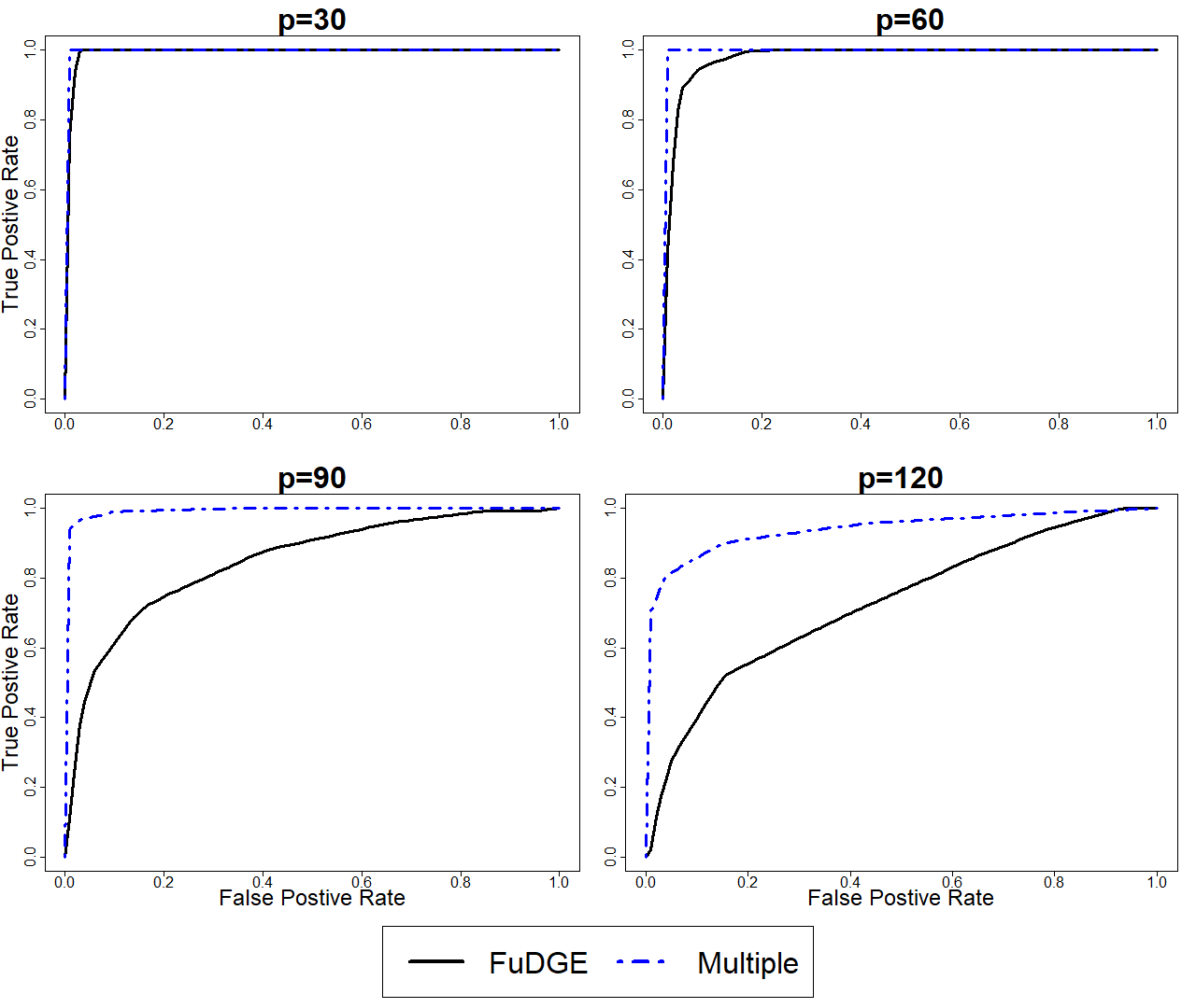
Here, data are generated with nX=nY=100n_{X}=n_{Y}=100, and p=30,60,90,120p=30,60,90,120. We repeat the simulation 30 times for each pp. The model setting here is similar to model 2 in Section 4.1. However, we make two major changes. First, when we generate the functional variables, we use a 5-dimensional Fourier basis, so that all basis are supported over the entire interval, rather than disjoint support as in Section 4.1. Second, we set matrix WW to be diagonal. Specifically, we let Wk​k=cW_{kk}=c for k=1,2,⋯,5k=1,2,\cdots,5 and Wk​m=0W_{km}=0 for k≠mk\neq m, where cc is drawn uniformly from [0.6,1][0.6,1], and scaled by 1/21/2 for p=30p=30, 1/31/3 for p=60p=60, and 1/41/4 for p=90p=90. All other settings are the same. The average ROC curves are shown in Figure 2, and the mean area under the curves are shown in Table 2 in section D.2 of supplementary material.
Refer to caption
Figure 2: Average ROC curves across 30 simulations of example that multiple network strategy works better

In Section 4.1 we considered extreme settings where the data must be treated as functions, and here we consider an extreme setting where the functional nature is irrelevant. In practice, however, the data may often lie between these two settings, and the method which performs better should depend on the variation of the differential structure across time. However, as it may be hard to measure this variation in practice, treating the data as functional objects should be a more robust choice.

4.3 Neuroscience application

We apply our method to electroencephalogram (EEG) data obtained from an alcoholism study [29, 6, 18] which included 122 total subjects; 77 in an alcoholic group and 45 in the control group. Specifically, the EEG data was measured by placing p=64p=64 electrodes on various locations on the subject’s scalp and measuring voltage values across time. We follow the preprocessing procedure in [8, 31], which filters the EEG signals at α\alpha frequency bands between 8 and 12.5 Hz.

[18] separately estimate functional graphs for both groups, but we directly estimate the differential graph using FuDGE. We choose λn\lambda_{n} so that the estimated differential graph has approximately 1% of possible edges. The estimated edges of the differential graph are shown in Figure 3.

Refer to caption
Figure 3: Estimated differential graph for EEG data. The anterior region is the top of the figure and the posterior region is the bottom of the figure.

We see that edges are generally between nodes located in the same region–either the anterior region or the posterior region–and there is no edge that crosses between regions. This observation is consistent with the result in [18] where there are no connections between frontal and back regions for both groups. We also note that electrode CZ, lying in the central region has a high degree in the estimated differential graph. While there is no direct connection between anterior and posterior regions, the central region may play a role in helping the two parts communicate.

5 Discussion

In this paper, we propose a method to directly estimate the differential graph for functional graphical models. In certain settings, direct estimation allows for the differential graph to be recovered consistently, even if each underlying graph cannot be consistently recovered. Experiments on simulated data also show that preserving the functional nature of the data rather than treating the data as multivariate scalars can also result in better estimation of the difference graph.

A key step in the procedure is first representing the functions with an MM-dimensional basis using FPCA, and Assumption 3.2 ensures that there exists some MM large enough so that the signal, τ\tau, is larger than the bias due to using a finite dimensional representation, ν\nu. Intuitively, ν\nu is tied to the eigenvalue decay rate; however, we defer derivation of the explicit connection for future work. Finally, we have provided a method for direct estimation of the differential graph, but development of methods which allow for inference and hypothesis testing in functional differential graphs would be fruitful avenues for future work. For example, [7] has developed inference tools for high-dimensional Markov networks, future works may extend their results to functional graph setting.

Appendix A Derivation of optimization algorithm

In this section we derive the closed-form updates for the proximal method stated in (2.11). In particular, recall that for all 1≤j,l≤p1\leq{j,l}\leq{p}

Δj​lnew=[(‖Aj​lold‖F−λn​η)/‖Aj​lold‖F]+×Aj​lold,\Delta^{\text{new}}_{jl}\;=\;\left[\left(\|A^{\text{old}}_{jl}\|_{F}-\lambda_{n}\eta\right)/\|A^{\text{old}}_{jl}\|_{F}\right]_{+}\times A^{\text{old}}_{jl},

where Aold=Δold−η∇L(Δold)A^{\text{old}}=\Delta^{\text{old}}-\eta\nabla L(\Delta^{\text{old}}) and x+=max⁡{0,x},x∈ℝx_{+}=\max\{0,x\},x\in{\mathbb{R}} represents the positive part of xx.

Proof of (2.11).

Let Aold=Δold−η∇L(Δold)A^{\text{old}}=\Delta^{\text{old}}-\eta\nabla L(\Delta^{\text{old}}), and let fj​lf_{jl} denote the loss decomposed over each j,lj,l block so that

fj​l​(Δj​l)=12​λn​η​‖Δj​l−Aj​lold‖F2+‖Δj​l‖F,{}f_{jl}(\Delta_{jl})\;=\;\frac{1}{2\lambda_{n}\eta}\|\Delta_{jl}-A^{\text{old}}_{jl}\|^{2}_{F}+\|\Delta_{jl}\|_{F}, (A.1)

and

Δj​lnew=arg​minΔjl∈ℝM×M⁡fjl​(Δjl).\Delta^{\text{new}}_{jl}\;=\;\argmin_{\Delta_{jl}\in{\mathbb{R}^{M\times{M}}}}f_{jl}(\Delta_{jl}). (A.2)

The loss fj​l​(Δj​l)f_{jl}(\Delta_{jl}) is convex, so the first order optimality condition implies that:

0∈∂fj​l​(Δj​lnew),{}0\in\partial f_{jl}\left(\Delta^{\text{new}}_{jl}\right), (A.3)

where ∂fj​l​(Δj​l)\partial f_{jl}\left(\Delta_{jl}\right) is the subdifferential of fj​lf_{jl} at Δj​l\Delta_{jl}. Note that ∂fj​l​(Δj​l)\partial f_{jl}\left(\Delta_{jl}\right) can be expressed as:

∂fj​l​(Δj​l)=1λn​η​(Δj​l−Aj​lold)+Zj​l,{}\partial f_{jl}(\Delta_{jl})\;=\;\frac{1}{\lambda_{n}\eta}\left(\Delta_{jl}-A^{\text{old}}_{jl}\right)+Z_{jl}, (A.4)

where

Zj​l={Δj​l‖Δj​l‖F if ​Δj​l≠0{Zj​l∈ℝM×M:‖Zj​l‖F≤1} if ​Δj​l=0.{}Z_{jl}\;=\;\begin{cases}\frac{\Delta_{jl}}{\|\Delta_{jl}\|_{F}}\qquad&\text{ if }\Delta_{jl}\neq{0}\\[10.0pt] \left\{Z_{jl}\in{\mathbb{R}^{M\times{M}}}\colon\|Z_{jl}\|_{F}\leq{1}\right\}\qquad&\text{ if }\Delta_{jl}=0.\end{cases} (A.5)

Claim 1 If ‖Aj​lold‖F>λn​η>0\|A^{\text{old}}_{jl}\|_{F}>\lambda_{n}\eta>0, then Δj​lnew≠0\Delta^{\text{new}}_{jl}\neq{0}.

We verify this claim by proving the contrapositive. Suppose Δj​lnew=0\Delta^{\text{new}}_{jl}={0}, then by (A.3) and (A.5), there exists a Zj​l∈ℝM×MZ_{jl}\in{\mathbb{R}^{M\times{M}}} such that ‖Zj​l‖F≤1\|Z_{jl}\|_{F}\leq{1} and

0=−1λn​η​Aj​lold+Zj​l.0=-\frac{1}{\lambda_{n}\eta}A^{\text{old}}_{jl}+Z_{jl}.

Thus,

‖Aj​lold‖F=‖λn​η⋅Zj​l‖F≤λn​η,\|A^{\text{old}}_{jl}\|_{F}=\|\lambda_{n}\eta\cdot Z_{jl}\|_{F}\leq{\lambda_{n}\eta},

so that Claim 1 holds.

Combining Claim 1 with (A.3) and (A.5), for any j,lj,l such that ‖Aj​lold‖F>λn​η\|A^{\text{old}}_{jl}\|_{F}>\lambda_{n}\eta, we have

0=1λn​η​(Δj​lnew−Aj​lold)+Δj​lnew‖Δj​lnew‖F,0=\frac{1}{\lambda_{n}\eta}\left(\Delta^{\text{new}}_{jl}-A^{\text{old}}_{jl}\right)+\frac{\Delta^{\text{new}}_{jl}}{\|\Delta^{\text{new}}_{jl}\|_{F}},

which is solved by

Δj​lnew=‖Aj​lold‖F−λn​η‖Aj​lold‖F​Aj​lold.{}\Delta^{\text{new}}_{jl}=\frac{\|A^{\text{old}}_{jl}\|_{F}-\lambda_{n}\eta}{\|A^{\text{old}}_{jl}\|_{F}}A^{\text{old}}_{jl}. (A.6)

Claim 2 If ‖Aj​lold‖F≤λn​η\|A^{\text{old}}_{jl}\|_{F}\leq\lambda_{n}\eta, then Δj​lnew=0\Delta^{\text{new}}_{jl}=0.

Again, we verify the claim by proving the contrapositive. Suppose Δj​lnew≠0\Delta^{\text{new}}_{jl}\neq 0, then first order optimality implies the updates in (A.6). However, taking the Frobenius norm of both sides of the equation gives ‖Δj​lnew‖F=‖Aj​lold‖F−λn​η\|\Delta^{\text{new}}_{jl}\|_{F}=\|A^{\text{old}}_{jl}\|_{F}-\lambda_{n}\eta which implies that ‖Aj​lold‖F−λn​η≥0\|A^{\text{old}}_{jl}\|_{F}-\lambda_{n}\eta\geq{0}.

The updates in (2.11) immediately follow from combining Claim 2 and (A.6). ∎

Appendix B Proof of theoretical properties

We provide the proof of Theorem 3.1, which states that under certain conditions, our estimator consistently recovers EΔE_{\Delta}. We follow the framework introduced in [15], but first introduce some necessary notation.

We use ⊗\otimes to denote the Kronecker product. For Δ∈ℝp​M×p​M\Delta\in\mathbb{R}^{pM\times pM}, let θ=vec⁡(Δ)∈ℝp2​M2\theta=\vect(\Delta)\in{\mathbb{R}^{p^{2}M^{2}}} and θ∗=vec⁡(ΔM)\theta^{*}=\vect({\Delta^{M}}), where ΔM\Delta^{M} is defined in Section 2.2. Let 𝒢={Gt}t=1,…,N𝒢\mathcal{G}=\{G_{t}\}_{t=1,\ldots,N_{\mathcal{G}}} be a set of indices, where N𝒢=p2N_{\mathcal{G}}=p^{2} and Gt⊂{1,2,⋯,p2​M2}G_{t}\subset\{1,2,\cdots,p^{2}M^{2}\} is the set of indices for θ\theta which correspond to the tt-th M×MM\times M submatrix of ΔM\Delta^{M}. Thus, if t=(j−1)​p+lt=(j-1)p+l, then θGt=vec⁡(Δj​l)∈ℝM2\theta_{G_{t}}=\vect{(\Delta_{jl})}\in{\mathbb{R}^{M^{2}}} where Δj​l\Delta_{jl} is the (j,l)(j,l)-th M×MM\times{M} submatrix of Δ\Delta. Denote the group indices of θ∗\theta^{*} that belong to blocks corresponding to EΔE_{\Delta} as S𝒢⊆{1,2,⋯,N𝒢}S_{\mathcal{G}}\subseteq{\{1,2,\cdots,N_{\mathcal{G}}\}}. Note that we define S𝒢S_{\mathcal{G}} using EΔE_{\Delta} and not EΔME_{\Delta^{M}}, so as stated in Assumption 3.3, |S𝒢|=s|S_{\mathcal{G}}|=s. We further define the subspace ℳ\mathcal{M} as

ℳ≔{θ∈ℝp2​M2|θGt=0​ for all ​t∉S𝒢},{}\mathcal{M}\coloneqq{\{\theta\in{\mathbb{R}^{p^{2}M^{2}}}|\theta_{G_{t}}=0\text{ for all }t\notin{S_{\mathcal{G}}}\}}, (B.1)

and its orthogonal complement with respect to the usual Euclidean inner product is

ℳ⊥≔{θ∈ℝp2​M2|θGt=0​ for all ​t∈S𝒢}.\mathcal{M}^{\bot}\coloneqq{\{\theta\in{\mathbb{R}^{p^{2}M^{2}}}|\theta_{G_{t}}=0\text{ for all }t\in{S_{\mathcal{G}}}\}}. (B.2)

For a vector θ\theta, let θℳ\theta_{\mathcal{M}} and θℳ⊥\theta_{\mathcal{M}^{\bot}} be the projection of θ\theta on the subspaces ℳ\mathcal{M} and ℳ⊥\mathcal{M}^{\bot}, respectively. Let ⟨⋅,⋅⟩\langle\cdot,\cdot\rangle represent the usual Euclidean inner product. Let

ℛ⁡(θ)≔∑t=1N𝒢|θGt|2≜‖θ‖1,2.{}\mathcal{R}(\theta)\coloneqq{\sum_{t=1}^{N_{\mathcal{G}}}|\theta_{G_{t}}|_{2}}\triangleq{\|\theta\|_{1,2}}. (B.3)

For any v∈ℝp2​M2v\in{\mathbb{R}^{p^{2}M^{2}}}, the dual norm of ℛ\mathcal{R} is given by

ℛ∗​(v)≔supu∈ℝp2​M2\{0}⟨u,v⟩ℛ⁡(u)=supℛ⁡(u)≤1⟨u,v⟩,{}\mathcal{R}^{*}(v)\coloneqq\sup_{u\in{\mathbb{R}^{p^{2}M^{2}}\backslash{\{0\}}}}\frac{\langle{u},{v}\rangle}{\mathcal{R}(u)}=\sup_{\mathcal{R}(u)\leq{1}}\langle{u},{v}\rangle, (B.4)

and the subspace compatibility constant of ℳ\mathcal{M} with respect to ℛ\mathcal{R} is defined as

Ψ⁡(ℳ)≔supu∈ℳ\{0}ℛ⁡(u)|u|2.{}\Psi(\mathcal{M})\coloneqq{\sup_{u\in{\mathcal{M}\backslash\{0\}}}}\frac{\mathcal{R}(u)}{|u|_{2}}. (B.5)

B.1 Proof of theoreom 3.1

Let σm​a​x=max⁡{|ΣX,M|∞,|ΣY,M|∞}\sigma_{max}=\max\{|\Sigma^{X,M}|_{\infty},\ |\Sigma^{Y,M}|_{\infty}\}. Suppose that

|SX,M−ΣX,M|∞\displaystyle|S^{X,M}-\Sigma^{X,M}|_{\infty} ≤δ,\displaystyle\leq\delta, (B.6)
|SY,M−ΣY,M|∞\displaystyle|S^{Y,M}-\Sigma^{Y,M}|_{\infty} ≤δ,\displaystyle\leq\delta,

for some appropriate choice of δ\delta. Then

|(SY,M⊗SX,M)−(ΣY,M⊗ΣX,M)|∞≤δ2+2​δ​σm​a​x,|(S^{Y,M}\otimes{S^{X,M}})-(\Sigma^{Y,M}\otimes{\Sigma^{X,M}})|_{\infty}\leq\delta^{2}+2\delta\sigma_{max}, (B.7)

and

|vec⁡(SY,M−SX,M)−vec⁡(ΣY,M−ΣX,M)|∞≤2​δ.|\vect{(S^{Y,M}-S^{X,M})}-\vect{(\Sigma^{Y,M}-\Sigma^{X,M})}|_{\infty}\leq 2\delta. (B.8)

Because by assumption limM→∞ν⁡(M)=0\lim_{M\rightarrow\infty}\nu(M)=0, there exists some MM large enough so that 2​ν​(M)<τ2\nu(M)<\tau, for τ\tau defined in Assumption 3.2. In particular, we suppose for such MM, that δ<14​λm​i​n∗+16​M2​s​(σm​a​x)2M2​s−σm​a​x\delta<\frac{1}{4}\sqrt{\frac{\lambda^{*}_{min}+16M^{2}s(\sigma_{max})^{2}}{M^{2}s}}-\sigma_{max}. Later, we show using Lemma C.2 that this occurs with high probability for large nn.

Problem (2.7) can be written in following form:

θ^λn∈arg​minθ∈ℝp2​M2⁡ℒ​(θ)+λn​ℛ​(θ),\hat{\theta}_{\lambda_{n}}\in\argmin_{\theta\in{\mathbb{R}^{p^{2}M^{2}}}}\mathcal{L}(\theta)+\lambda_{n}\mathcal{R}(\theta), (B.9)

where

ℒ⁡(θ)=12​θT​(SY,M⊗SX,M)​θ−θT​vec⁡(SY,M−SX,M).{}\mathcal{L}(\theta)=\frac{1}{2}\theta^{T}(S^{Y,M}\otimes{S^{X,M}})\theta-\theta^{T}\vect({S^{Y,M}-S^{X,M}}). (B.10)

The loss ℒ⁡(θ)\mathcal{L}(\theta) is convex and differentiable with respect to θ\theta, and it can be easily verified that ℛ⁡(⋅)\mathcal{R}(\cdot) defines a vector norm. For h∈ℝp2​M2h\in\mathbb{R}^{p^{2}M^{2}}, the error of the first-order Taylor series expansion of ℒ\mathcal{L} is:

δ​ℒ​(h,θ∗)\displaystyle\delta{\mathcal{L}}(h,\theta^{*}) ≔ℒ⁡(θ∗+h)−ℒ⁡(θ∗)−⟨∇ℒ​(θ∗),h⟩\displaystyle\coloneqq\mathcal{L}(\theta^{*}+h)-\mathcal{L}(\theta^{*})-\langle\nabla\mathcal{L}(\theta^{*}),h\rangle (B.11)
=12​hT​(SY,M⊗SX,M)​h.\displaystyle=\frac{1}{2}h^{T}(S^{Y,M}\otimes{S^{X,M}})h.

Using the form of (B.10), we see that ∇ℒ​(θ)=(SY,M⊗SX,M)​θ−vec⁡(SY,M−SX,M)\nabla{\mathcal{L}}(\theta)=(S^{Y,M}\otimes{S^{X,M}})\theta-\vect({S^{Y,M}-S^{X,M}}), and by Lemma C.1, we have

ℛ∗​(∇ℒ​(θ∗))=maxt=1,2,⋯,N𝒢⁡|[(SY,M⊗SX,M)​θ∗−vec⁡(SY,M−SX,M)]Gt|2.{}\mathcal{R}^{*}(\nabla{\mathcal{L}}(\theta^{*}))=\max_{t=1,2,\cdots,N_{\mathcal{G}}}\left|\left[(S^{Y,M}\otimes{S^{X,M}})\theta^{*}-\vect({S^{Y,M}-S^{X,M}})\right]_{G_{t}}\right|_{2}. (B.12)

We now show an upper bound for ℛ∗​(∇ℒ​(θ∗))\mathcal{R}^{*}(\nabla{\mathcal{L}}(\theta^{*})). First, note that

(ΣY,M⊗ΣX,M)​θ∗−vec⁡(ΣY,M−ΣX,M)=vec⁡(ΣX,M​ΔM​ΣY,M−(ΣY,M−ΣX,M))=0.(\Sigma^{Y,M}\otimes{\Sigma^{X,M}})\theta^{*}-\vect({\Sigma^{Y,M}-\Sigma^{X,M}})=\vect({\Sigma^{X,M}\Delta^{M}\Sigma^{Y,M}-(\Sigma^{Y,M}-\Sigma^{X,M})})=0.

Letting (⋅)j​l(\cdot)_{jl} denote the (j,l)(j,l)-th submatrix, we have

|[(SY,M⊗SX,M)​θ∗−vec⁡(SY,M−SX,M)]Gt|2\displaystyle\left|\left[(S^{Y,M}\otimes{S^{X,M}})\theta^{*}-\vect({S^{Y,M}-S^{X,M}})\right]_{G_{t}}\right|_{2} (B.13)
=|[(SY,M⊗SX,M−ΣY,M⊗ΣX,M)​θ∗−vec⁡((SY,M−ΣY,M)−(SX,M−ΣX,M))]Gt|2\displaystyle=\left|\left[(S^{Y,M}\otimes{S^{X,M}}-\Sigma^{Y,M}\otimes{\Sigma^{X,M}})\theta^{*}-\vect{((S^{Y,M}-\Sigma^{Y,M})-(S^{X,M}-\Sigma^{X,M}))}\right]_{G_{t}}\right|_{2}
≤‖(SX,M​ΔM​SY,M−ΣX,M​ΔM​ΣY,M)j​l−(SY,M−ΣY,M)j​l−(SX,M−ΣX,M)j​l‖F\displaystyle\leq{\|(S^{X,M}\Delta^{M}S^{Y,M}-\Sigma^{X,M}\Delta^{M}\Sigma^{Y,M})_{jl}-(S^{Y,M}-\Sigma^{Y,M})_{jl}-(S^{X,M}-\Sigma^{X,M})_{jl}\|_{F}}
≤‖(SX,M​ΔM​SY,M−ΣX,M​ΔM​ΣY,M)j​l‖F+‖(SY,M−ΣY,M)j​l‖F+‖(SX,M−ΣX,M)j​l‖F.\displaystyle\leq{\|(S^{X,M}\Delta^{M}S^{Y,M}-\Sigma^{X,M}\Delta^{M}\Sigma^{Y,M})_{jl}\|_{F}+\|(S^{Y,M}-\Sigma^{Y,M})_{jl}\|_{F}+\|(S^{X,M}-\Sigma^{X,M})_{jl}\|_{F}}.

For any M×MM\times{M} matrix AA, ‖A‖F≤M​|A|∞\|A\|_{F}\leq{M|A|_{\infty}}, so

|[(SY,M⊗SX,M)​θ∗−vec⁡(SY,M−SX,M)]Gt|2\displaystyle\left|\left[(S^{Y,M}\otimes{S^{X,M}})\theta^{*}-\vect({S^{Y,M}-S^{X,M}})\right]_{G_{t}}\right|_{2}
≤M[|(SX,MΔMSY,M−ΣX,MΔMΣY,M)j​l|∞+|(SY,M−ΣY,M)j​l|∞\displaystyle\leq M\left[\left|(S^{X,M}\Delta^{M}S^{Y,M}-\Sigma^{X,M}\Delta^{M}\Sigma^{Y,M})_{jl}\right|_{\infty}+\left|(S^{Y,M}-\Sigma^{Y,M})_{jl}\right|_{\infty}\right.
+|(SX,M−ΣX,M)j​l|∞]\displaystyle\left.\hskip 10.00002pt+\left|(S^{X,M}-\Sigma^{X,M})_{jl}\right|_{\infty}\right]
≤M⁡[|SX,M​ΔM​SY,M−ΣX,M​ΔM​ΣY,M|∞+|SY,M−ΣY,M|∞+|​SX,M−ΣX,M|∞].\displaystyle\leq M\left[\left|S^{X,M}\Delta^{M}S^{Y,M}-\Sigma^{X,M}\Delta^{M}\Sigma^{Y,M}\right|_{\infty}+|S^{Y,M}-\Sigma^{Y,M}|_{\infty}+|S^{X,M}-\Sigma^{X,M}|_{\infty}\right].

Now, note that for any A∈ℝk×kA\in{\mathbb{R}^{k\times{k}}} and v∈ℝkv\in{\mathbb{R}^{k}}, we have |A​v|∞≤|A|∞|​v|1|Av|_{\infty}\leq{|A|_{\infty}|v|_{1}}, thus we further have

|SX,M​ΔM​SY,M−ΣX,M​ΔM​ΣY,M|∞\displaystyle|S^{X,M}\Delta^{M}S^{Y,M}-\Sigma^{X,M}\Delta^{M}\Sigma^{Y,M}|_{\infty} =|[(SY,M⊗SX,M)−(ΣX,M⊗ΣY,M)]​vec⁡(ΔM)|∞\displaystyle=|[(S^{Y,M}\otimes{S^{X,M}})-(\Sigma^{X,M}\otimes{\Sigma^{Y,M}})]\vect{(\Delta^{M})}|_{\infty}
≤|(SY,M⊗SX,M)−(ΣX,M⊗ΣY,M)|∞|​vec⁡(ΔM)|1\displaystyle\leq{|(S^{Y,M}\otimes{S^{X,M}})-(\Sigma^{X,M}\otimes{\Sigma^{Y,M}})|_{\infty}}|\vect{(\Delta^{M})}|_{1}
=|(SY,M⊗SX,M)−(ΣX,M⊗ΣY,M)|∞|​ΔM|1.\displaystyle=|(S^{Y,M}\otimes{S^{X,M}})-(\Sigma^{X,M}\otimes{\Sigma^{Y,M}})|_{\infty}|\Delta^{M}|_{1}.

Combining the inequalities gives an upper bound uniform over 𝒢\mathcal{G} (i.e., for all GtG_{t}):

|[(SY,M⊗SX,M)​θ∗−vec⁡(SY,M−SX,M)]Gt|2\displaystyle\left|\left[(S^{Y,M}\otimes{S^{X,M}})\theta^{*}-\vect({S^{Y,M}-S^{X,M}})\right]_{G_{t}}\right|_{2}
≤M[|(SY,M⊗SX,M)−(ΣX,M⊗ΣY,M)|∞|ΔM|1+|SY,M−ΣY,M|∞\displaystyle\leq M\left[|(S^{Y,M}\otimes{S^{X,M}})-(\Sigma^{X,M}\otimes{\Sigma^{Y,M}})|_{\infty}|\Delta^{M}|_{1}+|S^{Y,M}-\Sigma^{Y,M}|_{\infty}\right.
+|SX,M−ΣX,M|∞],\displaystyle\left.\hskip 10.00002pt+|S^{X,M}-\Sigma^{X,M}|_{\infty}\right],

which implies

ℛ∗​(∇ℒ​(θ∗))\displaystyle\mathcal{R}^{*}\left(\nabla{\mathcal{L}}(\theta^{*})\right) ≤M[|(SY,M⊗SX,M)−(ΣX,M⊗ΣY,M)|∞|ΔM|1+|SY,M−ΣY,M|∞\displaystyle\leq M\left[|(S^{Y,M}\otimes{S^{X,M}})-(\Sigma^{X,M}\otimes{\Sigma^{Y,M}})|_{\infty}|\Delta^{M}|_{1}+|S^{Y,M}-\Sigma^{Y,M}|_{\infty}\right. (B.14)
+|SX,M−ΣX,M|∞].\displaystyle\left.\hskip 10.00002pt+|S^{X,M}-\Sigma^{X,M}|_{\infty}\right].

Assuming |SX,M−ΣX,M|∞≤δ|S^{X,M}-\Sigma^{X,M}|_{\infty}\leq{\delta} and |SY,M−ΣY,M|∞≤δ|S^{Y,M}-\Sigma^{Y,M}|_{\infty}\leq\delta implies

ℛ∗​(∇ℒ​(θ∗))≤M⁡[(δ2+2​δ​σm​a​x)​|ΔM|1+2​δ],{}\mathcal{R}^{*}\left(\nabla{\mathcal{L}}(\theta^{*})\right)\leq{M[(\delta^{2}+2\delta\sigma_{max})|\Delta^{M}|_{1}+2\delta]}, (B.15)

where 0<δ≤c10<\delta\leq{c_{1}}.

Setting

λn=2​M​[(δ2+2​δ​σm​a​x)​|ΔM|1+2​δ],{}\lambda_{n}=2M\left[\left(\delta^{2}+2\delta\sigma_{max}\right)\left|\Delta^{M}\right|_{1}+2\delta\right], (B.16)

then implies that λn≥2​ℛ∗​(∇ℒ​(θ∗))\lambda_{n}\geq{2\mathcal{R}^{*}\left(\nabla{\mathcal{L}}(\theta^{*})\right)}. Thus, invoking Lemma 1 in [15], h=θ^λn−θ∗h=\hat{\theta}_{\lambda_{n}}-\theta^{*} must satisfy

ℛ⁡(hℳ⊥)≤3​ℛ​(hℳ)+4​ℛ​(θℳ⊥∗),{}\mathcal{R}(h_{\mathcal{M}^{\bot}})\leq{3\mathcal{R}(h_{\mathcal{M}})}+4\mathcal{R}(\theta^{*}_{\mathcal{M}^{\bot}}), (B.17)

where ℳ\mathcal{M} is defined in (B.1). Equivalently,

‖hℳ⊥‖1,2≤3​‖hℳ‖1,2+4​‖θℳ⊥∗‖1,2.{}\|h_{\mathcal{M}^{\bot}}\|_{1,2}\leq{3\|h_{\mathcal{M}}\|_{1,2}}+4\|\theta^{*}_{\mathcal{M}^{\bot}}\|_{1,2}. (B.18)

By the definition of ν\nu in Assumption 3.2, we have

‖θℳ⊥∗‖1,2=∑t∉𝒮𝒢‖θGt∗‖2≤(p⁡(p+1)/2−s)​ν≤p2​ν.{}\|\theta^{*}_{\mathcal{M}^{\bot}}\|_{1,2}=\sum_{t\notin{\mathcal{S}_{\mathcal{G}}}}\|\theta^{*}_{G_{t}}\|_{2}\leq\left(p(p+1)/2-s\right)\nu\leq p^{2}\nu. (B.19)

Next, we show that δ​ℒ​(h,θ∗)\delta\mathcal{L}(h,\theta^{*}), as defined in (B.11), satisfies the Restricted Strong Convexity property defined in definition 2 in [15]. That is, we show an inequality of the form: δ​ℒ​(h,θ∗)≥κℒ​|h|22−ωℒ2​(θ∗)\delta\mathcal{L}(h,\theta^{*})\geq{\kappa_{\mathcal{L}}|h|^{2}_{2}}-\omega^{2}_{\mathcal{L}}\left(\theta^{*}\right) whenever hh satisfies (B.18).

By using Lemma C.3, we have

θT​(SY,M⊗SX,M)​θ\displaystyle\theta^{T}(S^{Y,M}\otimes{S^{X,M}})\theta =θT​(ΣY,M⊗ΣX,M)​θ+θT​(SY,M⊗SX,M−ΣY,M⊗ΣX,M)​θ\displaystyle=\theta^{T}(\Sigma^{Y,M}\otimes{\Sigma^{X,M}})\theta+\theta^{T}(S^{Y,M}\otimes{S^{X,M}}-\Sigma^{Y,M}\otimes{\Sigma^{X,M}})\theta
≥θT​(ΣY,M⊗ΣX,M)​θ−|θT​(SY,M⊗SX,M−ΣY,M⊗ΣX,M)​θ|\displaystyle\geq{\theta^{T}(\Sigma^{Y,M}\otimes{\Sigma^{X,M}})\theta-|\theta^{T}(S^{Y,M}\otimes{S^{X,M}}-\Sigma^{Y,M}\otimes{\Sigma^{X,M}})\theta|}
≥λm​i​n∗​|θ|22−M2|​SY,M⊗SX,M−ΣY,M⊗ΣX,M|∞​‖θ‖1,22,\displaystyle\geq{\lambda^{*}_{min}}|\theta|^{2}_{2}-M^{2}|S^{Y,M}\otimes{S^{X,M}}-\Sigma^{Y,M}\otimes{\Sigma^{X,M}}|_{\infty}\|\theta\|^{2}_{1,2},

where the last inequality holds because Lemma C.3 and λm​i​n∗=λm​i​n​(ΣX,M)×λm​i​n​(ΣY,M)=λm​i​n​(ΣY,M⊗ΣX,M)>0\lambda^{*}_{min}=\lambda_{min}(\Sigma^{X,M})\times{\lambda_{min}(\Sigma^{Y,M})}=\lambda_{min}(\Sigma^{Y,M}\otimes{\Sigma^{X,M}})>0. Thus,

δ​ℒ​(h,θ∗)\displaystyle\delta\mathcal{L}(h,\theta^{*}) =12​hT​(SY,M⊗SX,M)​h\displaystyle=\frac{1}{2}h^{T}(S^{Y,M}\otimes{S^{X,M}})h
≥12​λm​i​n∗​|h|22−12​M2|​SY,M⊗SX,M−ΣY,M⊗ΣX,M|∞​‖h‖1,22.\displaystyle\geq{\frac{1}{2}\lambda^{*}_{min}}|h|^{2}_{2}-\frac{1}{2}M^{2}|S^{Y,M}\otimes{S^{X,M}}-\Sigma^{Y,M}\otimes{\Sigma^{X,M}}|_{\infty}\|h\|^{2}_{1,2}.

By Lemma C.4 and (B.18), we have

‖h‖1,22\displaystyle\|h\|^{2}_{1,2} =(‖hℳ‖1,2+‖hℳ⊥‖1,2)2\displaystyle=(\|h_{\mathcal{M}}\|_{1,2}+\|h_{\mathcal{M}^{\bot}}\|_{1,2})^{2}
≤16​(‖hℳ‖1,2+‖θℳ⊥∗‖1,2)2\displaystyle\leq 16({\|h_{\mathcal{M}}\|_{1,2}}+\|\theta^{*}_{\mathcal{M}^{\bot}}\|_{1,2})^{2}
≤16​(s​‖h‖2+p2​ν)2\displaystyle\leq 16(\sqrt{s}\|h\|_{2}+p^{2}\nu)^{2}
≤32​s​‖h‖22+32​p2​ν.\displaystyle\leq 32s\|h\|^{2}_{2}+32p^{2}\nu.

Combining with the equation above, we get

δ​ℒ​(h,θ∗)\displaystyle\delta\mathcal{L}(h,\theta^{*}) ≥[12​λmin∗−16​M2​s​|SY,M⊗SX,M−ΣY,M⊗ΣX,M|∞]​|h|22\displaystyle\geq{\left[\frac{1}{2}\lambda^{*}_{\min}-16M^{2}s|S^{Y,M}\otimes{S^{X,M}}-\Sigma^{Y,M}\otimes{\Sigma^{X,M}}|_{\infty}\right]}|h|^{2}_{2} (B.20)
−16​M2​p4​ν2​|SY,M⊗SX,M−ΣY,M⊗ΣX,M|∞\displaystyle-16M^{2}p^{4}\nu^{2}|S^{Y,M}\otimes{S^{X,M}}-\Sigma^{Y,M}\otimes{\Sigma^{X,M}}|_{\infty}
≥[12​λmin∗−8​M2​s​(δ1​δ2+δ2​σmax+δ1​σmaxY)]​|h|22\displaystyle\geq\left[\frac{1}{2}\lambda^{*}_{\min}-8M^{2}s\left(\delta_{1}\delta_{2}+\delta_{2}\sigma_{\max}+\delta_{1}\sigma^{Y}_{\max}\right)\right]|h|^{2}_{2}
−16​M2​p4​ν2​(δ1​δ2+δ2​σmax+δ1​σmaxY).\displaystyle-16M^{2}p^{4}\nu^{2}\left(\delta_{1}\delta_{2}+\delta_{2}\sigma_{\max}+\delta_{1}\sigma^{Y}_{\max}\right).

Thus, appealing to (B.7), the Restricted Strong Convexity property holds with

κℒ\displaystyle\kappa_{\mathcal{L}} =12​λm​i​n∗−8​M2​s​(δ2+2​δ​σm​a​x),\displaystyle=\;\frac{1}{2}\lambda^{*}_{min}-8M^{2}s\left(\delta^{2}+2\delta\sigma_{max}\right), (B.21)
ωℒ\displaystyle\omega_{\mathcal{L}} = 4​M​p2​ν​δ2+2​δ​σm​a​x.\displaystyle=\;4Mp^{2}\nu\sqrt{\delta^{2}+2\delta\sigma_{max}}.

When δ<14​λm​i​n∗+16​M2​s​(σm​a​x)2M2​s−σm​a​x\delta<\frac{1}{4}\sqrt{\frac{\lambda^{*}_{min}+16M^{2}s(\sigma_{max})^{2}}{M^{2}s}}-\sigma_{max} then κℒ>0\kappa_{\mathcal{L}}>0. By Theorem 1 of [15] and Lemma C.4, letting λn=2​M​[(δ2+2​δ​σm​a​x)​|ΔM|1+2​δ]\lambda_{n}=2M\left[\left(\delta^{2}+2\delta\sigma_{max}\right)|\Delta^{M}|_{1}+2\delta\right], as in (B.16), ensures

‖Δ^M−ΔM‖F2\displaystyle\|\hat{\Delta}^{M}-\Delta^{M}\|^{2}_{F} =‖θ^λn−θ∗‖22\displaystyle=\|\hat{\theta}_{\lambda_{n}}-\theta^{*}\|^{2}_{2} (B.22)
≤9​λn2κℒ2​Ψ2​(ℳ)+λnκℒ​(2​ωℒ2+4​ℛ​(θℳ⊥∗))\displaystyle\leq{9\frac{\lambda^{2}_{n}}{\kappa^{2}_{\mathcal{L}}}}\Psi^{2}(\mathcal{M})+\frac{\lambda_{n}}{\kappa_{\mathcal{L}}}\left(2\omega^{2}_{\mathcal{L}}+4\mathcal{R}(\theta^{*}_{\mathcal{M}^{\bot}})\right)
=9​λn2​sκℒ2+2​λnκℒ​(ωℒ2+2​p2​ν)\displaystyle=\frac{9\lambda^{2}_{n}s}{\kappa^{2}_{\mathcal{L}}}+\frac{2\lambda_{n}}{\kappa_{\mathcal{L}}}(\omega^{2}_{\mathcal{L}}+2p^{2}\nu)
≔Γ.\displaystyle\coloneqq\Gamma.

Note that Γ\Gamma is function of δ\delta through λn\lambda_{n} (defined in (B.16)), κℒ\kappa_{\mathcal{L}}, and ωℒ\omega_{\mathcal{L}}. For fixed MM, ν⁡(M)\nu(M) and pp, k→0k\rightarrow 0 as δ→0\delta\rightarrow 0, so there exists a δ0>0\delta_{0}>0 such that δ<δ0\delta<\delta_{0} implies

Γ\displaystyle\Gamma <(1/2)​τ−ν,\displaystyle<(1/2)\tau-\nu, (B.23)
δ\displaystyle\delta <min⁡{14​λm​i​n∗+16​M2​s​(σm​a​x)2M2​s−σm​a​x,c13/2},\displaystyle<\min\left\{\frac{1}{4}\sqrt{\frac{\lambda^{*}_{min}+16M^{2}s(\sigma_{max})^{2}}{M^{2}s}}-\sigma_{max},\;c_{1}^{3/2}\right\},

for any c1>0c_{1}>0. When these hold, there exists an

ϵn∈(Γ+ν,τ−(Γ+ν)),\epsilon_{n}\in\left(\Gamma+\nu,\tau-(\Gamma+\nu)\right), (B.24)

and when thresholding with this ϵn\epsilon_{n} we claim E^ΔM=EΔ\hat{E}_{\Delta^{M}}=E_{\Delta}. We prove this claim below.

Note that we have ‖Δ^j​l−Δj​lM‖F≤‖Δ^−ΔM‖F≤Γ\|\hat{\Delta}_{jl}-\Delta^{M}_{jl}\|_{F}\leq{\|\hat{\Delta}-\Delta^{M}\|_{F}}\leq\Gamma for any (j,l)∈V2(j,l)\in{V^{2}}. Recall that

EΔ={(j,l)∈V2:∥Cj​lΔ∥HS>0,j≠l}.{}E_{\Delta}\;=\;\{(j,l)\in{V^{2}}:\;\|C^{\Delta}_{jl}\|_{\text{HS}}>0,j\neq{l}\}. (B.25)

We first prove that EΔ⊆E^ΔME_{\Delta}\subseteq{\hat{E}_{{\Delta}^{M}}}. For any (j,l)∈EΔ(j,l)\in{E_{\Delta}}, by the definition of ν\nu and τ\tau in Assumption 3.2, we have ‖Cj​lΔ‖HS≥τ\|C^{\Delta}_{jl}\|_{\text{HS}}\geq{\tau} and ‖Δj​lM‖F≥‖Cj​lΔ‖HS−ν\|\Delta^{M}_{jl}\|_{F}\geq{\|C^{\Delta}_{jl}\|_{\text{HS}}-\nu}. Thus, we have

‖Δ^j​l‖F\displaystyle\|\hat{\Delta}_{jl}\|_{F} ≥‖Δj​lM‖F−‖Δ^j​l−Δj​lM‖F\displaystyle\geq{\|\Delta^{M}_{jl}\|_{F}-\|\hat{\Delta}_{jl}-\Delta^{M}_{jl}\|_{F}}
≥‖Cj​lΔ‖HS−‖Δ^j​l−Δj​lM‖F−ν\displaystyle\geq{\|C^{\Delta}_{jl}\|_{\text{HS}}-\|\hat{\Delta}_{jl}-\Delta^{M}_{jl}\|_{F}-\nu}
≥τ−Γ−ν\displaystyle\geq{\tau-\Gamma-\nu}
>ϵn.\displaystyle>\epsilon_{n}.

The last inequality holds because we have assumed that ϵn∈(Γ+ν⁡(M),τ−(Γ+ν⁡(M)))\epsilon_{n}\in\left(\Gamma+\nu(M),\tau-(\Gamma+\nu(M))\right). Thus, by definition of E^ΔM\hat{E}_{{\Delta}^{M}} shown in (2.9), we have (j,l)∈E^ΔM(j,l)\in{\hat{E}_{{\Delta}^{M}}} which further implies that EΔ⊆E^ΔME_{\Delta}\subseteq{\hat{E}_{{\Delta}^{M}}}.

We then show E^ΔM⊆EΔ\hat{E}_{{\Delta}^{M}}\subseteq{E_{\Delta}}. Let E^ΔMc\hat{E}^{c}_{{\Delta}^{M}} and EΔcE^{c}_{\Delta} denote the complement set of E^ΔM\hat{E}_{{\Delta}^{M}} and EΔE_{\Delta}. For any (j,l)∈EΔc(j,l)\in{E^{c}_{\Delta}}, which also means that (l,j)∈EΔc(l,j)\in{E^{c}_{\Delta}}, by (B.25), we have ‖Cj​lΔ‖HS=0\|C^{\Delta}_{jl}\|_{\text{HS}}=0, thus

‖Δ^j​l‖F\displaystyle\|\hat{\Delta}_{jl}\|_{F} ≤‖Δj​lM‖F+‖Δ^j​l−Δj​lM‖F\displaystyle\leq{\|\Delta^{M}_{jl}\|_{F}+\|\hat{\Delta}_{jl}-\Delta^{M}_{jl}\|_{F}}
≤‖Cj​lΔ‖HS+‖Δ^j​l−Δj​lM‖F+ν\displaystyle\leq{\|C^{\Delta}_{jl}\|_{\text{HS}}+\|\hat{\Delta}_{jl}-\Delta^{M}_{jl}\|_{F}}+\nu
≤Γ+ν\displaystyle\leq\Gamma+\nu
<ϵn.\displaystyle<\epsilon_{n}.

Again, the last inequality holds because because we have assumed that ϵn\epsilon_{n} satisfies (B.24). Thus, by definition of E^ΔM\hat{E}_{{\Delta}^{M}}, we have (j,l)∉E^ΔM(j,l)\notin{\hat{E}_{{\Delta}^{M}}} or (j,l)∈E^ΔMc(j,l)\in{\hat{E}^{c}_{{\Delta}^{M}}}. This implies that EΔc⊆E^ΔMcE^{c}_{\Delta}\subseteq{\hat{E}^{c}_{{\Delta}^{M}}}, or E^ΔM⊆EΔ\hat{E}_{{\Delta}^{M}}\subseteq{E_{\Delta}}. Combing with previous conclusion that EΔ⊆E^ΔME_{\Delta}\subseteq{\hat{E}_{{\Delta}^{M}}}, the proof is complete.

We now show that for any δ\delta, there exists some nn large enough so that, (B.6), (B.7) and (B.8) occur with high probability. In particular, let

δ=M1+βX​2​(log⁡p+log⁡M+log⁡n)n,\delta\;=\;M^{1+\beta_{X}}\sqrt{\frac{2\left(\log{p}+\log{M}+\log{n}\right)}{n}}, (B.26)

where limn→∞δ⁡(n)=0\lim_{n\rightarrow\infty}\delta(n)=0. Thus, there exists some nn large enough such that δ0=δ⁡(n)\delta_{0}=\delta(n) satisfies (B.23). Then, Lemma C.2 implies that there exists some c1c_{1}, c2c_{2} such that (B.6), (B.7) and (B.8) holds for δ<c1\delta<c_{1} with probability 1−2​c2/n21-2c_{2}/n^{2}.

Appendix C Lemmas in the proof of theoretical properties

Lemma C.1.

For ℛ⁡(⋅)\mathcal{R}(\cdot) norm defined in (B.3), its dual norm ℛ∗​(⋅)\mathcal{R}^{*}(\cdot), defined in (B.4), is

ℛ∗​(v)=maxt=1,…,N𝒢⁡|vGt|2.\mathcal{R}^{*}(v)\;=\;\max_{t=1,\ldots,N_{\mathcal{G}}}|v_{G_{t}}|_{2}. (C.1)
Proof.

For any u:‖u‖1,2≤1u:\|u\|_{1,2}\leq{1} and v∈ℝp2​M2v\in{\mathbb{R}^{p^{2}M^{2}}}, we have

⟨v,u⟩\displaystyle\langle{v,u}\rangle =∑t=1N𝒢⟨vGt,uGt⟩\displaystyle=\sum_{t=1}^{N_{\mathcal{G}}}\langle{v_{G_{t}},u_{G_{t}}}\rangle
≤∑t=1N𝒢|vGt|2|​uGt|2\displaystyle\leq{\sum_{t=1}^{N_{\mathcal{G}}}|v_{G_{t}}|_{2}|u_{G_{t}}|_{2}}
≤(maxt=1,2,⋯,N𝒢⁡|vGt|2)​∑t=1N𝒢|uGt|2\displaystyle\leq\left(\max_{t=1,2,\cdots,N_{\mathcal{G}}}|v_{G_{t}}|_{2}\right)\sum_{t=1}^{N_{\mathcal{G}}}|u_{G_{t}}|_{2}
=(maxt=1,2,⋯,N𝒢⁡|vGt|2)​‖u‖1,2\displaystyle=\left(\max_{t=1,2,\cdots,N_{\mathcal{G}}}|v_{G_{t}}|_{2}\right)\|u\|_{1,2}
≤maxt=1,2,⋯,N𝒢⁡|vGt|2.\displaystyle\leq{\max_{t=1,2,\cdots,N_{\mathcal{G}}}|v_{G_{t}}|_{2}}.

To complete the proof, we to show that this upper bound can be obtained. Let t∗=arg​maxt=1,2,⋯,N𝒢⁡|vGt|t^{*}=\argmax_{t=1,2,\cdots,N_{\mathcal{G}}}|v_{G_{t}}|, and select uu such that

uGt\displaystyle u_{G_{t}} =0\displaystyle=0 ∀t≠t∗,\displaystyle\hskip 20.00003pt{\forall{t\neq{t^{*}}}},
uGt\displaystyle u_{G_{t}} =vGt∗|vGt∗|2\displaystyle=\frac{v_{G_{t^{*}}}}{|v_{G_{t^{*}}}|_{2}} t=t∗.\displaystyle\hskip 20.00003pt{t={t^{*}}}.

It follows that ‖u‖1,2=1\|u\|_{1,2}=1 and ⟨v,u⟩=|vGt∗|2=maxt=1,…,N𝒢⁡|vGt|2\langle{v,u}\rangle=|v_{G_{t^{*}}}|_{2}=\max_{t=1,\ldots,N_{\mathcal{G}}}|v_{G_{t}}|_{2}. ∎

Lemma C.2.

Let

f⁡(n,p,M,δ,β,c1,c2)=c2​p2​M2​exp⁡{−c1​n​M−(2+2​β)​δ2},f\left(n,p,M,\delta,\beta,c_{1},c_{2}\right)\;=\;c_{2}p^{2}M^{2}\exp\left\{-c_{1}nM^{-(2+2\beta)}\delta^{2}\right\}, (C.2)

β=min⁡{βX,βY}\beta=\min\{\beta_{X},\beta_{Y}\} where βX\beta_{X} and βY\beta_{Y} are as defined in Assumption 3.1, and σm​a​x=max⁡{σm​a​xX,σm​a​xY}\sigma_{max}=\max\{\sigma^{X}_{max},\sigma^{Y}_{max}\} where σm​a​xX\sigma^{X}_{max} and σm​a​xY\sigma^{Y}_{max} are as defined in Section 3.

There exists positive constants, c1c_{1} and c2c_{2}, such that for 0<δ<c10<\delta<c_{1}, with probability at least 1−2​f​(min⁡{nX,nY},p,M,δ,β,c1,c2)1-2f\left(\min\{n_{X},n_{Y}\},p,M,\delta,\beta,c_{1},c_{2}\right) the following statements hold simultaneously:

|SX,M−ΣX,M|∞\displaystyle|S^{X,M}-\Sigma^{X,M}|_{\infty} ≤δ,\displaystyle\leq\delta, (C.3)
|SY,M−ΣY,M|∞\displaystyle|S^{Y,M}-\Sigma^{Y,M}|_{\infty} ≤δ,\displaystyle\leq\delta,
|(SY,M⊗SX,M)−(ΣY,M⊗ΣX,M)|∞≤δ2+2​δ​σm​a​x,|(S^{Y,M}\otimes{S^{X,M}})-(\Sigma^{Y,M}\otimes{\Sigma^{X,M}})|_{\infty}\leq\delta^{2}+2\delta\sigma_{max}, (C.4)

and

|vec⁡(SY,M−SX,M)−vec⁡(ΣY,M−ΣX,M)|∞≤2​δ.{}|\vect{(S^{Y,M}-S^{X,M})}-\vect{(\Sigma^{Y,M}-\Sigma^{X,M})}|_{\infty}\leq 2\delta. (C.5)
Proof.

Denote the (j,l)(j,l)-th M×MM\times M submatrix of SX,MS^{X,M} by Sj​lX,MS^{X,M}_{jl} and the (k,m)(k,m)-th entry of Sj​lX,MS^{X,M}_{jl} by σ^j​l,k​mX,M\hat{\sigma}^{X,M}_{jl,km} for j,l=1,…,pj,l=1,\ldots,p and k,m=1,…,Mk,m=1,\ldots,M. We use similar notation for ΣX,M\Sigma^{X,M}, SY,MS^{Y,M}, and ΣY,M\Sigma^{Y,M}.

The statement in (C.3) holds directly by applying Theorem 1 in [18] to SX,MS^{X,M} and SY,MS^{Y,M} and combining the statements with a union bound.

To show (C.4), note that (C.3) then implies

|σ^j​l,k​mX,M​σ^j′​l′,k′​m′Y,M−Σj​l,k​mX,M​σj′​l′,k′​m′Y,M|\displaystyle|\hat{\sigma}^{X,M}_{jl,km}\hat{\sigma}^{Y,M}_{j^{\prime}l^{\prime},k^{\prime}m^{\prime}}-\Sigma^{X,M}_{jl,km}\sigma^{Y,M}_{j^{\prime}l^{\prime},k^{\prime}m^{\prime}}| ≤|σ^j​l,k​mX,M−σj​l,k​mX,M|​|σ^j′​l′,k′​m′Y,M−σj′​l′,k′​m′Y,M|\displaystyle\leq{|\hat{\sigma}^{X,M}_{jl,km}-\sigma^{X,M}_{jl,km}||\hat{\sigma}^{Y,M}_{j^{\prime}l^{\prime},k^{\prime}m^{\prime}}-\sigma^{Y,M}_{j^{\prime}l^{\prime},k^{\prime}m^{\prime}}|}
+|σ^j​l,k​mX,M|​|σ^j′​l′,k′​m′Y,M−σj′​l′,k′​m′Y,M|\displaystyle+|\hat{\sigma}^{X,M}_{jl,km}||\hat{\sigma}^{Y,M}_{j^{\prime}l^{\prime},k^{\prime}m^{\prime}}-\sigma^{Y,M}_{j^{\prime}l^{\prime},k^{\prime}m^{\prime}}|
+|σ^j′​l′,k′​m′Y,M|​|σ^j​l,k​mX,M−σj​l,k​mX,M|\displaystyle+|\hat{\sigma}^{Y,M}_{j^{\prime}l^{\prime},k^{\prime}m^{\prime}}||\hat{\sigma}^{X,M}_{jl,km}-\sigma^{X,M}_{jl,km}|
≤|SX,M−ΣX,M|∞|​SY,M−ΣY,M|∞\displaystyle\leq|S^{X,M}-\Sigma^{X,M}|_{\infty}|S^{Y,M}-\Sigma^{Y,M}|_{\infty}
+σm​a​x​|SY,M−ΣY,M|∞+σm​a​x​|SX,M−ΣX,M|\displaystyle+\sigma_{max}|S^{Y,M}-\Sigma^{Y,M}|_{\infty}+\sigma_{max}|S^{X,M}-\Sigma^{X,M}|
≤δ2+2​δ​σm​a​x.\displaystyle\leq\delta^{2}+2\delta\sigma_{max}.

For (C.5), note that

|vec⁡(SY,M−SX,M)−vec⁡(ΣY,M−ΣX,M)|∞\displaystyle|\vect{(S^{Y,M}-S^{X,M})}-\vect{(\Sigma^{Y,M}-\Sigma^{X,M})}|_{\infty} =|(SX,M−ΣX,M)−(SY,M−ΣY,M)|∞\displaystyle=|(S^{X,M}-\Sigma^{X,M})-(S^{Y,M}-\Sigma^{Y,M})|_{\infty}
≤|SX,M−ΣX,M|∞+|​SY,M−ΣY,M|∞\displaystyle\leq|S^{X,M}-\Sigma^{X,M}|_{\infty}+|S^{Y,M}-\Sigma^{Y,M}|_{\infty}
≤2​δ.\displaystyle\leq 2\delta.

∎

Lemma C.3.

For a set of indices 𝒢={Gt}t=1,…,N𝒢\mathcal{G}=\{G_{t}\}_{t=1,\ldots,N_{\mathcal{G}}}, suppose ∥⋅∥1,2\|\cdot\|_{1,2} is defined in (B.3). Then for any matrix A∈ℝp2​M2×p2​M2A\in{\mathbb{R}^{p^{2}M^{2}\times{p^{2}M^{2}}}} and θ∈ℝp2​M2\theta\in{\mathbb{R}^{p^{2}M^{2}}}

|θT​A​θ|≤M2​|A|∞​‖θ‖1,22.|\theta^{T}A\theta|\leq{M^{2}|A|_{\infty}\|\theta\|^{2}_{1,2}}. (C.6)
Proof.
|θT​A​θ|\displaystyle|\theta^{T}A\theta| =|∑i∑jAi​j​θi​θj|\displaystyle=\left|\sum_{i}\sum_{j}A_{ij}\theta_{i}\theta_{j}\right|
≤∑i∑j|Ai​j​θi​θj|\displaystyle\leq{\sum_{i}\sum_{j}|A_{ij}\theta_{i}\theta_{j}|}
≤|A|∞​(∑i|θi|)2\displaystyle\leq{|A|_{\infty}\left(\sum_{i}|\theta_{i}|\right)^{2}}
=|A|∞​(∑t=1N𝒢∑k∈Gt|θk|)2\displaystyle=|A|_{\infty}\left(\sum_{t=1}^{N_{\mathcal{G}}}\sum_{k\in{G_{t}}}|\theta_{k}|\right)^{2}
=|A|∞​(∑t=1N𝒢‖θGt‖1)2\displaystyle=|A|_{\infty}\left(\sum_{t=1}^{N_{\mathcal{G}}}\|\theta_{G_{t}}\|_{1}\right)^{2}
≤|A|∞​(∑t=1N𝒢M​‖θGt‖2)2\displaystyle\leq{|A|_{\infty}\left(\sum_{t=1}^{N_{\mathcal{G}}}M\|\theta_{G_{t}}\|_{2}\right)^{2}}
=M2​|A|∞​‖θ‖1,22.\displaystyle=M^{2}|A|_{\infty}\|\theta\|^{2}_{1,2}.

In the penultimate line, we use the property that for any vector v∈ℝnv\in{\mathbb{R}^{n}}, |v|1≤n​|v|2|v|_{1}\leq{\sqrt{n}|v|_{2}}. ∎

Lemma C.4.

Suppose ℳ\mathcal{M} is defined as in (B.1). For any θ∈ℳ\theta\in{\mathcal{M}}, we have ‖θ‖1,2≤s​|θ|2\|\theta\|_{1,2}\leq{\sqrt{s}}|\theta|_{2}. Furthermore, for Ψ⁡(ℳ)\Psi(\mathcal{M}) as defined in (B.5), we have Ψ⁡(ℳ)=s\Psi(\mathcal{M})=\sqrt{s}.

Proof.

By definition of ℳ\mathcal{M} and ∥⋅∥1,2\|\cdot\|_{1,2}, we have

‖θ‖1,2\displaystyle\|\theta\|_{1,2} =∑t∈S𝒢|θGt|2+∑t∉S𝒢|θGt|2\displaystyle=\sum_{t\in{S_{\mathcal{G}}}}|\theta_{G_{t}}|_{2}+\sum_{t\notin{S_{\mathcal{G}}}}|\theta_{G_{t}}|_{2}
=∑t∈S𝒢|θGt|2\displaystyle=\sum_{t\in{S_{\mathcal{G}}}}|\theta_{G_{t}}|_{2}
≤s​(∑t∈S𝒢|θGt|22)12\displaystyle\leq{\sqrt{s}}\left(\sum_{t\in{S_{\mathcal{G}}}}|\theta_{G_{t}}|^{2}_{2}\right)^{\frac{1}{2}}
=s​|θ|2.\displaystyle=\sqrt{s}|\theta|_{2}.

In the penultimate line, we appeal to the Cauchy-Schwartz inequality. To show Ψ⁡(ℳ)=s\Psi(\mathcal{M})=\sqrt{s}, it suffices to show that the upper bound above can be achieved. Select θ∈ℝp2​M2\theta\in{\mathbb{R}^{p^{2}M^{2}}} such that |θGt|2=c|\theta_{G_{t}}|_{2}=c, ∀t∈S𝒢\forall{t\in{S_{\mathcal{G}}}}, where cc is some positive constant. This implies that ‖θ‖1,2=s​c\|\theta\|_{1,2}=sc and |θ|2=s​c|\theta|_{2}=\sqrt{s}c so that ‖θ‖1,2=s​|θ|2\|\theta\|_{1,2}=\sqrt{s}|\theta|_{2}. Thus, Ψ⁡(ℳ)=s\Psi(\mathcal{M})=\sqrt{s}.

∎

Appendix D More simulation results

D.1 AUC table of simulations in section 4.1

Table 1: The mean area under the ROC curves. Standard errors are shown in parentheses.
FuDGE AIC BIC Multiple
pp Model1
30 0.99 (0.01) 0.75 (0.17) 0.5 (0) 0.71 (0.11)
60 0.91 (0.06) 0.5 (0) 0.5 (0) 0.56 (0.1)
90 0.82 (0.1) 0.5(0) 0.5 (0) 0.55 (0.09)
120 0.64 (0.06) 0.5(0) 0.5 (0) 0.53 (0.04)
pp Model2
30 0.9 (0.08) 0.59 (0.06) 0.5 (0) 0.53 (0.14)
60 0.9 (0.07) 0.5 (0) 0.5 (0) 0.48 (0.11)
90 0.88 (0.08) 0.5(0) 0.5 (0) 0.46 (0.08)
120 0.86 (0.07) 0.5(0) 0.5 (0) 0.46 (0.12)
pp Model3
30 0.87 (0.06) 0.69 (0.06) 0.5 (0) 0.83 (0.08)
60 0.83 (0.09) 0.58 (0.07) 0.5 (0) 0.77 (0.09)
90 0.74 (0.1) 0.5(0) 0.5 (0) 0.57 (0.1)
120 0.74 (0.08) 0.5(0.02) 0.5 (0) 0.55 (0.05)

D.2 AUC table of simulations in section 4.2

Table 2: The mean area under the ROC curves of example that multiple network strategy works better. Standard errors are shown in parentheses
pp FuDGE Multiple
30 0.99 (0) 1 (0)
60 0.98 (0.01) 1 (0)
90 0.87 (0.09) 1 (0.01)
120 0.73 (0.12) 0.94 (0.09)

References

  • Beck and Teboulle [2009] A. Beck and M. Teboulle. A fast iterative shrinkage-thresholding algorithm for linear inverse problems. SIAM J. Imag. Sci., 2:183–202, 2009.
  • Bosq [2000] D. Bosq. Linear processes in function spaces, volume 149 of Lecture Notes in Statistics. Springer-Verlag, New York, 2000. Theory and applications.
  • Cai [2017] T. T. Cai. Global testing and large-scale multiple testing for high-dimensional covariance structures. Annual Review of Statistics and Its Application, 4(1):423–446, 2017.
  • Drton and Maathuis [2017] M. Drton and M. H. Maathuis. Structure learning in graphical modeling. Annual Review of Statistics and Its Application, 4:365–393, 2017.
  • Hsing and Eubank [2015] T. Hsing and R. Eubank. Theoretical foundations of functional data analysis, with an introduction to linear operators. Wiley Series in Probability and Statistics. John Wiley & Sons, Ltd., Chichester, 2015.
  • Ingber [1997] L. Ingber. Statistical mechanics of neocortical interactions: Canonical momenta indicators of electroencephalography. Physical Review E, 55(4):4578–4593, 1997.
  • Kim et al. [2019] B. Kim, S. Liu, and M. Kolar. Two-sample inference for high-dimensional markov networks. arXiv preprint arXiv:1905.00466, 2019.
  • Knyazev [2007] G. G. Knyazev. Motivation, emotion, and their inhibitory control mirrored in brain oscillations. Neuroscience & Biobehavioral Reviews, 31(3):377–395, 2007.
  • Kolar et al. [2010] M. Kolar, L. Song, A. Ahmed, and E. P. Xing. Estimating Time-varying networks. Ann. Appl. Stat., 4(1):94–123, 2010.
  • Lauritzen [1996] S. L. Lauritzen. Graphical Models, volume 17 of Oxford Statistical Science Series. The Clarendon Press Oxford University Press, New York, 1996. Oxford Science Publications.
  • Li and Solea [2018] B. Li and E. Solea. A nonparametric graphical model for functional data with application to brain networks based on fMRI. J. Amer. Statist. Assoc., 113(524):1637–1655, 2018.
  • Liu et al. [2014] S. Liu, J. A. Quinn, M. U. Gutmann, T. Suzuki, and M. Sugiyama. Direct learning of sparse changes in Markov networks by density ratio estimation. Neural Comput., 26(6):1169–1197, 2014.
  • Meinshausen and Bühlmann [2006] N. Meinshausen and P. Bühlmann. High dimensional graphs and variable selection with the lasso. Ann. Stat., 34(3):1436–1462, 2006.
  • Na et al. [2019] S. Na, M. Kolar, and O. Koyejo. Estimating differential latent variable graphical models with applications to brain connectivity. arXiv preprint arXiv:1909.05892, 2019.
  • Negahban et al. [2012] S. N. Negahban, P. Ravikumar, M. J. Wainwright, and B. Yu. A unified framework for high-dimensional analysis of mm-estimators with decomposable regularizers. Stat. Sci., 27(4):538–557, 2012.
  • Newman [2003] M. E. J. Newman. The structure and function of complex networks. SIAM Rev., 45(2):167–256, 2003.
  • Parikh and Boyd [2014] N. Parikh and S. P. Boyd. Proximal algorithms. Foundations and Trends in Optimization, 1(3):127–239, 2014.
  • Qiao et al. [2019] X. Qiao, S. Guo, and G. M. James. Functional Graphical Models. J. Amer. Statist. Assoc., 114(525):211–222, 2019.
  • Tibshirani [2010] R. Tibshirani. Proximal gradient descent and acceleration. Lecture Notes, 2010.
  • Wang et al. [2016] J.-L. Wang, J.-M. Chiou, and H.-G. Müller. Functional data analysis. Annual Review of Statistics and Its Application, 3(1):257–295, 2016.
  • Wang et al. [2018] Y. Wang, C. Squires, A. Belyaeva, and C. Uhler. Direct estimation of differences in causal graphs. In S. Bengio, H. M. Wallach, H. Larochelle, K. Grauman, N. Cesa-Bianchi, and R. Garnett, editors, Advances in Neural Information Processing Systems 31: Annual Conference on Neural Information Processing Systems 2018, NeurIPS 2018, 3-8 December 2018, Montréal, Canada., pages 3774–3785, 2018.
  • Xu and Gu [2016] P. Xu and Q. Gu. Semiparametric differential graph models. In D. D. Lee, M. Sugiyama, U. V. Luxburg, I. Guyon, and R. Garnett, editors, Advances in Neural Information Processing Systems 29, pages 1064–1072. Curran Associates, Inc., 2016.
  • Yao and Lee [2006] F. Yao and T. C. M. Lee. Penalized spline models for functional principal component analysis. J. R. Stat. Soc. Ser. B Stat. Methodol., 68(1):3–25, 2006.
  • Yu et al. [2016] M. Yu, V. Gupta, and M. Kolar. Statistical inference for pairwise graphical models using score matching. In Advances in Neural Information Processing Systems 29. Curran Associates, Inc., 2016.
  • Yu et al. [2019] M. Yu, V. Gupta, and M. Kolar. Simultaneous inference for pairwise graphical models with generalized score matching. arXiv preprint arXiv:1905.06261, 2019.
  • Yuan et al. [2017] H. Yuan, R. Xi, C. Chen, and M. Deng. Differential network analysis via lasso penalized D-trace loss. Biometrika, 104(4):755–770, 2017.
  • Yuan and Lin [2006] M. Yuan and Y. Lin. Model selection and estimation in regression with grouped variables. J. R. Stat. Soc. B, 68:49–67, 2006.
  • Zhang et al. [2018] C. Zhang, H. Yan, S. Lee, and J. Shi. Dynamic multivariate functional data modeling via sparse subspace learning. CoRR, abs/1804.03797, 2018, arXiv:1804.03797.
  • Zhang et al. [1995] X. L. Zhang, H. Begleiter, B. Porjesz, W. Wang, and A. Litke. Event related potentials during object recognition tasks. Brain Research Bulletin, 38(6):531–538, 1995.
  • Zhao et al. [2014] S. D. Zhao, T. T. Cai, and H. Li. Direct estimation of differential networks. Biometrika, 101(2):253–268, 2014.
  • Zhu et al. [2016] H. Zhu, N. Strawn, and D. B. Dunson. Bayesian graphical models for multivariate functional data. J. Mach. Learn. Res., 17:Paper No. 204, 27, 2016.