Learning to Map Natural Language Instructions to Physical Quadcopter Control using Simulated Flight
Abstract
We propose a joint simulation and real-world learning framework for mapping navigation instructions and raw first-person observations to continuous control. Our model estimates the need for environment exploration, predicts the likelihood of visiting environment positions during execution, and controls the agent to both explore and visit high-likelihood positions. We introduce Supervised Reinforcement Asynchronous Learning (SuReAL). Learning uses both simulation and real environments without requiring autonomous flight in the physical environment during training, and combines supervised learning for predicting positions to visit and reinforcement learning for continuous control. We evaluate our approach on a natural language instruction-following task with a physical quadcopter, and demonstrate effective execution and exploration behavior.
Keywords: Natural language understanding; quadcopter; uav; reinforcement learning; instruction following; observability; simulation; exploration;
1 Introduction
Controlling robotic agents to execute natural language instructions requires addressing perception, language, planning, and control challenges. The majority of methods addressing this problem follow such a decomposition, where separate components are developed independently and are then combined together [1, 2, 3, 4, 5, 6, e.g.,]. This requires a hard-to-scale engineering intensive process of designing and working with intermediate representations, including a formal language to represent natural language meaning. Recent work instead learns intermediate representations, and uses a single model to address all reasoning challenges [7, 8, 9, 10, e.g.,]. So far, this line of work has mostly focused on pre-specified low-level tasks. In contrast, executing natural language instructions requires understanding sentence structure, grounding words and phrases to observations, reasoning about previously unseen tasks, and handling ambiguity and uncertainty.
In this paper, we address the problem of mapping natural language navigation instructions to continuous control of a quadcopter drone using representation learning. We present a neural network model to jointly reason about observations, natural language, and robot control, with explicit modeling of the agent’s plan and exploration of the environment. For learning, we introduce Supervised and Reinforcement Asynchronous Learning (SuReAL), a method for joint training in simulated and physical environments. Figure 2 illustrates our task and model.


We design our model to reason about partial observability and incomplete knowledge of the environment in instruction following. We explicitly model observed and unobserved areas, and the agent’s belief that the goal location implied by the instruction has been observed. During learning, we use an intrinsic reward to encourage behaviors that increase this belief, and penalize for indicating task completion while still believing the goal is unobserved.
SuReAL addresses two key learning challenges. First, flying in a physical environment at the scale needed for our complex learning task is both time-consuming and costly. We mitigate this problem using a simulated environment. However, in contrast to the common approach of domain transfer from simulated to physical environments [11, 12], we simultaneously train in both, while not requiring autonomous flight in the physical environment during training. Second, as each example requires a human instruction, it is prohibitively expensive to collect language data at the scale required for representation learning [13, 14]. This is unlike tasks where data can be collected without human interaction. We combine supervised and reinforcement learning (RL); the first to best use the limited language data, and the second to effectively leverage experience.
We evaluate our approach with a navigation task, where a quadcopter drone flies between landmarks following natural language instructions. We modify an existing natural language dataset [15] to create a new benchmark with long instructions, complex trajectories, and observability challenges. We evaluate using both automated metrics and human judgements of semantic correctness. To the best of our knowledge, this is the first demonstration of a physical quadcopter system that follows natural language instructions by mapping raw first-person images and pose estimates to continuous control. Our code, data, and demo videos are available at https://github.com/lil-lab/drif.
2 Technical Overview
Task
Our goal is to map natural language navigation instructions to continuous control of a quadcopter drone. The agent behavior is determined by a velocity controller setpoint , where is a forward velocity and is a yaw rate. The model generates actions at fixed intervals. An action is either the task completion action or a setpoint update . Given a setpoint update at time , we fix the controller setpoint that is maintained between actions. Given a start state and an instruction , an execution of length is a sequence , where is the state at time , are setpoint updates, and . The state includes the quadcopter pose, internal state, and all landmark locations.
Model
We assume access to raw first-person monocular observations and pose estimates. The agent does not have access to the world state. At time , the agent observes the agent context , where is the instruction and and are monocular first-person RGB images and 6-DOF agent poses observed at time . We base our model on the Position Visitation Network [16, PVN;] architecture, and introduce mechanisms for reasoning about observability and exploration and learning across simulated and real environments. The model operates in two stages: casting planning as predicting distributions over world positions indicating the probability of visiting a position during execution, and generating actions to visit high probability positions.
Learning
We train jointly in simulated and physical environments. We assume access to a simulator and demonstration sets in both environments, in the physical environment and in the simulation. We do not interact with the physical environment during training. Each dataset includes examples , where , is an instruction, and is a demonstration execution. We do not require the datasets to be aligned or provide demonstrations for the same set of instructions. We propose SuReAL, a learning approach that concurrently trains the two model stages in two separate processes. The planning stage is trained with supervised learning, while the action generation stage is trained with RL. The two processes exchange data and parameters. The trajectories collected during RL are added to the dataset used for supervised learning, and the planning stage parameters are periodically transferred to the RL process training the action generation stage. This allows the action generator to learn to execute the plans predicted by the planning stage, which itself is trained using on-policy observations collected from the action generator.
Evaluation
We evaluate on a test set of examples , where is an instruction, is a start state, and is a human demonstration. We use human evaluation to verify the generated trajectories are semantically correct with regard to the instruction. We also use automated metrics. We consider the task successful if the agent stops within a predefined Euclidean distance of the final position in . We evaluate the quality of generating the trajectory following the instruction using earth mover’s distance between and executed trajectories.
3 Related Work
Natural language instruction following has been extensively studied using hand-engineered symbolic intermediate representations of world state or instruction semantics with physical robots [1, 2, 3, 4, 17, 5, 18, 6, 19] and simulated agents [20, 21, 22, 23, 24, 25]. In contrast, we study trading off the symbolic representation design with representation learning from demonstrations.
Representation learning has been studied for executing specific tasks such as grasping [7, 8, 10], dexterous manipulation [26, 27], or continuous flight [9]. Our aim is to execute navigation tasks specified in natural language, including new tasks at test time. This problem was addressed with representation learning in discrete simulated environments [28, 29, 30, 15, 31, 32], and more recently with continuous simulations [16]. However, these methods were not demonstrated on physical robots. A host of problems combine to make this challenging, including grounding natural language to constantly changing observations, robustly bridging the gap between relatively high-level instructions to continuous control, and learning with limited language data and the high costs of robot usage.
Our model is based on the Position Visitation Network [16] architecture that incorporates geometric computation to represent language and observations in learned spatial maps. This approach is related to neural network models that construct maps [33, 34, 35, 36] or perform planning [37].
Our approach is aimed at a partial observability scenario and does not assume access to the complete system state. Understanding the instruction often requires identifying mentioned entities that are not initially visible. This requires exploration during task execution. Nyga et al. 2018 studied modeling incomplete information in instructions with a modular approach. In contrast, we jointly learn to infer the absence of necessary information and to remedy it via exploration.
4 Model
We model the policy with a neural network. At time , given the agent context , the policy outputs a stopping probability , a forward velocity , and an angular velocity . We decompose the architecture to two stages , where predicts the probability of visiting positions in the environment and generates the actions to visit high probability positions. The position visitation probabilities are continuously updated during execution to incorporate the most recent observations, and past actions directly affect the information available for future decisions. Our model is based on the PVN architecture [16]. We introduce several improvements, including explicit modeling of observability in both stages. Appendix B contains further model implementation details, including a detailed list of our improvements. Figure 3 illustrates our model for an example input.
Stage 1: Visitation Distribution Prediction
At time , the first stage generates two probability distributions: a trajectory-visitation distribution and a goal-visitation distribution . Both distributions assign probabilities to positions , where is the set of positions observed up to time and represents all yet-unobserved positions. The set is a discretized approximation of the continuous environment. This approximation enables efficient computation of the visitation distributions [16]. The trajectory-visitation distribution assigns high probability to positions the agent should go through during execution, and the goal-visitation distribution puts high probability on positions where the agent should to complete its execution. We add the special position to PVN to capture probability mass that should otherwise be assigned to positions not yet observed, for example when the goal position has not been observed yet.

The first stage combines a learned neural network and differentiable deterministic computations. The input instruction is mapped to a vector using a recurrent neural network (RNN). The input image is mapped to a feature map that captures spatial and semantic information using a convolutional neural network (CNN). The feature map is processed using a deterministic semantic mapping process [34] using a pinhole camera model and the agent pose to project onto the environment ground at zero elevation. The projected features are deterministically accumulated from previous timesteps to create a semantic map . represents each position with a learned feature vector aggregated from all past observations of that position. For example, in Figure 3, the banana and the white bush can be identified in the raw image features and the projected semantic map , where their representations are identical. We generate a language-conditioned grounding map by creating convolutional filters using the text representation and filtering . The two maps aim to provide different representation: aims for a language-agnostic environment representation and is intended to focus on the objects mentioned in the instruction. We use auxiliary objectives (Appendix C.4) to optimize each map to contain the intended information. We predict the two distributions using LingUNet [15], a language-conditioned variant of the UNet image reconstruction architecture [39], which takes as input the learned maps, and , and the instruction representation . Appendix B.1 provides a detailed description of this architecture.
We add two outputs to the original PVN design: an observability mask and a boundary mask . Both are computed deterministically given the agent pose estimate and the camera parameters, and are intended to aid exploration of the environment during instruction execution. assigns to each position in the environment if has been observed by the agent’s first-person camera by time , or otherwise. assigns to environment boundaries and to other positions. Together, the masks provide information about what parts of the environment remain to be explored.
Stage 2: Action Generation
The second stage is a control network that receives four inputs: a trajectory-visitation distribution , a goal-visitation visitation distribution , an observability mask , and a boundary mask . The four inputs are rotated to the current egocentric agent reference frame, and used to generate the output velocities using a learned neural network. Appendix B.2 describes the network architecture. The velocities are generated to visit high probability positions according to , and the probability is predicted to stop in a likely position according to . In the figure, shows the curved flight path, and identifies the goal right of the banana. Our addition of the two masks and the special position enables generating actions to explore the environment to reduce and . Figure 2 visualizes with a green bar, showing how it starts high, and decreases once the goal is observed at step .
5 Learning
We learn two sets of parameters: for the first stage and for the second stage . We use a simulation for all autonomous flight during learning, and jointly train for both the simulation and the physical environment. This includes training a simulation-specific first stage with additional parameters . The second stage model is used in both environments. We assume access to sets of training examples for the simulation and for the physical environment, where are instructions and are demonstration executions. The training examples are not spatially or temporally aligned between domains.
Our learning algorithm, Supervised and Reinforcement Asynchronous Learning (SuReAL), uses two concurrent asynchronous processes. Each process only updates the parameters of one stage. Process A uses supervised learning to estimate Stage 1 parameters for both environments: for the physical environment model and for . We use both and to update the model parameters. We use RL in Process B to learn the parameters of the second stage using an intrinsic reward function. We start learning using the provided demonstrations in and periodically replace execution trajectories with RL rollouts from Process B, keeping a single execution per instruction at any time. We warm-start by running Process A for iterations before launching Process B to make sure that Process B always receives as input sensible visitation predictions instead of noise. The model parameters are periodically synchronized by copying the simulation parameters of Stage 1 from Process A to B. For learning, we use a learning architecture (Figure 4) that extends our model to process simulation observations and adds a discriminator that encourages learning representations that are invariant to the type of visual input.

Process A: Supervised Learning for Visitation Prediction
We train and to: (a) minimize the KL-divergence between the predicted visitation distributions and reference distributions generated from the demonstrations, and (b) learn domain invariant visual representations that allow sharing of instruction grounding and execution between the two environments. We use demonstration executions in the real environment and in the simulated environment . The loss for executions from the physical environment and the simulation is:
| (1) |
where is the sequence of contexts observed by the agent during an execution and creates the gold-standard visitation distribution examples (i.e., Stage 1 outputs) for a context from the training data. The term aims to make the feature representation indistinguishable between real and simulated images. This allows the rest of the model to use either simulated or real observations interchangeably. is the approximated empirical Wasserstein distance between the visual feature distributions extracted from simulated and real agent contexts:
where is a Lipschitz continuous neural network discriminator with parameters that we train to output high values for simulated features and low values for real features [40, 41]. is the -th image in the agent context . The discriminator architecture is described in Appendix C.1.
Algorithm 1 shows the supervised optimization procedure. We alternate between updating the discriminator parameters , and the first stage model parameters and . At every iteration, we perform gradient updates of to maximize the Wasserstein loss (lines 5–10), and then perform a single gradient update to and to minimize supervised learning loss (lines 11–13). We send the simulation-specific parameters to the RL process every iterations (line 15).
Algorithm 2 Process B: Reinforcement Learning 1: Simulation dataset , second-stage model with parameters , value function with parameters , first-stage simulation model . 2: is a set of sentence-execution pairs including all instructions from , where each instruction is paired with an execution from , or if not in . and are shared with Process A. 3: for do 4: » Get the most recent update from Process A 5: 6: for do 7: » Sample simulator executions of instructions 8: 9: for do 10: » Sample state-action-return tuples and update 11: 12: 13: » Update executions to share with Process A 14: 15: return
Process B: Reinforcement Learning for Action Generation
We train the action generator using RL with an intrinsic reward. We use Proximal Policy Optimization [42, PPO;] to maximize the expected return. The learner has no access to an external task reward, but instead computes a reward from how well the agent follows the visitation distributions generated by the first stage:
where is the agent context at time and is the action. The reward is a weighted combination of five terms. The visitation reward is the per-timestep reduction in earth mover’s distance between the predicted distribution and an empirical distribution that assigns equal probability to every position visited until time . This smooth and dense reward encourages to follow the visitation distributions predicted by . The stop reward is only non-zero for , when it is the earth mover’s distance between the predicted goal distribution and an empirical stopping distribution that assigns the full probability mass to the stop position in the policy execution. The exploration reward combines a positive reward for reducing the belief that the goal has not been observed yet (i.e., reducing ) and a negative reward proportional to the probability that the goal position is unobserved according to . The action reward penalizes actions outside of the controller range. Finally, is negative per-step reward to encourage efficient execution. We provide the reward implementation details in Appendix C.3.
Algorithm 2 shows the RL procedure. At every iteration, we collect simulation executions using the policy (line 8). To sample setpoint updates we treat the existing output as the mean of a normal distribution, add variance prediction, and sample the two velocities from the predicted normal distributions. We perform PPO updates using the return and value estimates (lines 9–12). For every update, we sample state-action-return triplets from the collected trajectories, compute the PPO loss , update parameters , and update the parameters of the value function . We pass the sampled executions to Process A to allow the model to learn to predict the visitation distributions in a way that is robust to the agent actions (line 14).
6 Experimental Setup
We provide the complete implementation and experimental setup details in Appendix E.
Environment and Data
We use an Intel Aero quadcopter with a PX4 flight controller, and a Vicon motion capture system for pose estimates. For simulation, we use the quadcopter simulator from Blukis et al. 2018 that is based on Microsoft AirSim [43]. The environment size is 4.7x4.7m. We randomly create environments with 5–8 landmarks, selected randomly out of a set of 15. Figure 2 shows the real environment. We follow the crowdsourcing setup of Misra et al. 2018 to collect 997 paragraphs with 4,557 segments. We use 3,245/640/672 for training, development, and testing. We expand this data by concatenating consecutive segments to create more challenging instructions, including with exploration challenges [32]. Figure 2 shows an instruction made of two consecutive segments. The simulator dataset includes oracle demonstrations of all instructions, while the real-world dataset includes only 402 single-segment demonstrations. For evaluation in the physical environment, we sample 20 test paragraphs consisting of 93 single-segment and 73 two-segment instructions. We use both single and concatenated instructions for training, and test on each set separately. We also use the original Misra et al. 2018 data as additional simulation training data. Appendix D provides data statistics and further details.
Evaluation
We use human judgements to evaluate if the agent’s final position is correct with regard to the instruction (goal score) and how well the agent followed the path described by the instruction (path score). We present MTurk workers with an instruction and a top-down animation of the agent behavior, and ask for a 5-point Likert-scale score for the final position and trajectory correctness. We obtain five judgements per example per system. We also automatically measure (a) SR: success rate of stopping within 47cm of the correct position; and (b) EMD: earth mover’s distance in meters between the agent and demonstration trajectories. Appendix F provides more evaluation details.
Systems
We compare our approach, PVN2-SuReAL , with three non-learning and two learning baselines: (1) STOP: output the action without movement; (2) Average: take the average action for the average number of steps; (3) Oracle: a hand-crafted upper-bound expert policy that has access to the ground truth human demonstration; (4) PVN-BC the Blukis et al. 2018 PVN model trained with behavior cloning; and (5) PVN2-BC: our model trained with behavior cloning. The two behavior cloning systems require access to an oracle that provides velocity command output labels, in addition to demonstration data. SuReAL uses demonstrations, but does not require the oracle during learning. None of the learned systems use any oracle data at test time. All learned systems use the same training data and , and include the domain-adaptation loss (Equation 1).
7 Results

Figure 5 shows human evaluation Likert scores. Our model receives five-point scores 39.72% of the time for getting the goal right, and 37.8% of the time for the path. This is a 34.9% and 24.8% relative improvement compared to PVN2-BC, the next best system. This demonstrates the benefits of modeling observability, using SuReAL for training-time exploration, and using a reward function that trades-off task performance and test-time exploration. The Average baseline received only 5-point ratings in both path score and goal score, demonstrating the task difficulty.
We study how well our model addresses observability and exploration challenges. Figure 6 shows human path score judgements split to tasks where the goal is visible from the agent’s first-person view at start position (34 examples) and those where it is not and exploration is required (38 examples). Our approach outperforms the baselines in cases requiring exploration, but it is slightly outperformed by PVN2-BC in simple examples. This could be explained by our agent attempting to explore the environment in cases where it is not necessary.
 Figure 6: Human evaluation path score frequencies (Figure 5) decomposed by initially unobservable (top) or observable (bottom) goal location.
| Method | 1-segment | 2-segment | |||
|---|---|---|---|---|---|
| SR | EMD | SR | EMD | ||
| Test Results | |||||
| Real | Average | 37.0 | 0.42 | 16.7 | 0.71 |
| PVN-BC | 48.9 | 0.42 | 20.8 | 0.61 | |
| PVN2-BC | 52.2 | 0.37 | 29.2 | 0.59 | |
| PVN2-SuReAL | 56.5 | 0.34 | 30.6 | 0.52 | |
| [0.5pt/1pt] | Oracle | 100.0 | 0.17 | 91.7 | 0.23 |
| Sim | Average | 29.5 | 0.53 | 8.7 | 0.80 |
| PVN-BC | 64.1 | 0.31 | 37.5 | 0.59 | |
| PVN2-BC | 55.4 | 0.34 | 34.7 | 0.58 | |
| PVN2-SuReAL | 53.3 | 0.30 | 33.3 | 0.42 | |
| [0.5pt/1pt] | Oracle | 100.0 | 0.13 | 98.6 | 0.17 |
| Development Results | |||||
| Real | PVN2-SuReAL | 54.8 | 0.32 | 31.0 | 0.50 |
| PVN2-SuReAL-noU | 53.8 | 0.30 | 14.3 | 0.56 | |
| PVN2-SuReAL50real | 60.6 | 0.29 | 34.5 | 0.44 | |
| PVN2-SuReAL10real | 46.2 | 0.33 | 17.9 | 0.56 | |
| Sim | PVN2-SuReAL | 48.1 | 0.29 | 39.3 | 0.40 |
| PVN2-SuReAL-noU | 53.8 | 0.28 | 27.4 | 0.50 | |
| PVN2-SuReAL-noI | 56.2 | 0.28 | 25.9 | 0.45 | |
Table 1 shows the automated metrics for both environments. We observe that the success rate (SR) measure is sensitive to the threshold selection, and correct executions are often considered as wrong; PVN2-SuReAL gets 30.6% SR compared to a perfect human score 39.72% of the time. This highlights the need for human evaluation, and must be considered when interpreting the SR results. We generally find EMD more reliable, although it also does not account for semantic correctness.
Comparing to PVN2-BC, our approach performs better on the real environment demonstrating the benefit of SuReAL. In simulation, we observe better EMD, but worse SR. Qualitatively, we observe our approach often recovers the correct overall trajectory, with a slightly imprecise stopping location due to instruction ambiguity or control challenges. Such partial correctness is not captured by SR. Comparing PVN2-BC and PVN-BC, we see the benefit of modeling observability. SuReAL further improves upon PVN2-BC, by learning to explore unobserved locations at test-time.
Comparing our approach between simulated and real environments, we see an absolute performance degradation of 2.7% SR and 0.1 EMD from simulation to the real environment. This highlights the remaining challenges of visual domain transfer and complex flight dynamics. The flight dynamics challenges are also visible in the Oracle performance degradation between the two environments.
We study several ablations. First, we quantify the effect of using a smaller number of real-world training demonstrations. We randomly select subsets of demonstrations, with the constraint that all objects are visually represented. We find that using only half (200) of the physical demonstrations does not appear to reduce performance (), while using only 10% (40), drastically hurts real-world performance (). This shows that the learning method is successfully leveraging real-world data to improve performance, while requiring relatively modest amounts of data. We also study performance without access to the instruction (PVN2-SuReAL-noU), and with using a blank input image (PVN2-SuReAL-noI). The relatively high SR of these ablations on 1-segment instructions highlights the inherent bias in simple trajectories. The 2-segment data, which is our main focus, is much more robust to such biases. Appendix G provides more automatic evaluation results, including additional ablations and results on the original data of Misra et al. 2018.
8 Discussion
We study the problem of mapping natural language instructions to continuous control of a physical quadcopter drone. Our two-stage model decomposition allows some level of re-use and modularity. For example, a trained Stage 1 can be re-used with different robot types. This decomposition and the interpretability it enables also create limitations, including limited sensory input for deciding about control actions given the visitation distributions. These are both important topics for future study.
Our learning method, SuReAL, uses both annotated demonstration trajectories and a reward function. In this work, we assume demonstration trajectories were generated with an expert policy. However, SuReAL does not necessarily require the initial demonstrations to come from a reasonable policy, as long as we have access to the gold visitation distributions, which are easier to get compared to oracle actions. For example, given an initial policy that immediately stops instead of demonstrations, we will train Stage 1 to predict the given visitation distributions and Stage 2 using the intrinsic reward. Studying this empirically is an important direction for future work.
Finally, our environment provides a strong testbed for our system-building effort and the transition from the simulation to the real world. However, various problems are not well represented, such as reasoning about obstacles, raising important directions for future work. While we do not require the simulation to accurately reflect the real world, studying scenarios with stronger difference between the two is another important future direction. Our work also points towards the need for better automatic evaluation for instruction following, or, alternatively, wide adoption of human evaluation.
Acknowledgments
This research was supported by the generosity of Eric and Wendy Schmidt by recommendation of the Schmidt Futures program, a Google Faculty Award, NSF CAREER-1750499, AFOSR FA9550-17-1-0109, an Amazon Research Award, and cloud computing credits from Amazon. We thank Dipendra Misra, Alane Suhr, and the anonymous reviewers for their helpful comments.
References
- Tellex et al. [2011] S. Tellex, T. Kollar, S. Dickerson, M. R. Walter, A. Gopal Banerjee, S. Teller, and N. Roy. Approaching the Symbol Grounding Problem with Probabilistic Graphical Models. AI Magazine, 2011.
- Matuszek et al. [2012] C. Matuszek, N. FitzGerald, L. Zettlemoyer, L. Bo, and D. Fox. A Joint Model of Language and Perception for Grounded Attribute Learning. In ICML, 2012.
- Duvallet et al. [2013] F. Duvallet, T. Kollar, and A. Stentz. Imitation learning for natural language direction following through unknown environments. In ICRA, 2013.
- Walter et al. [2013] M. R. Walter, S. Hemachandra, B. Homberg, S. Tellex, and S. Teller. Learning Semantic Maps from Natural Language Descriptions. In RSS, 2013.
- Hemachandra et al. [2015] S. Hemachandra, F. Duvallet, T. M. Howard, N. Roy, A. Stentz, and M. R. Walter. Learning models for following natural language directions in unknown environments. In ICRA, 2015.
- Gopalan et al. [2018] N. Gopalan, D. Arumugam, L. L. Wong, and S. Tellex. Sequence-to-sequence language grounding of non-markovian task specifications. In RSS, 2018.
- Lenz et al. [2015] I. Lenz, H. Lee, and A. Saxena. Deep learning for detecting robotic grasps. IJRR, 2015.
- Levine et al. [2016] S. Levine, P. Pastor, A. Krizhevsky, and D. Quillen. Learning hand-eye coordination for robotic grasping with large-scale data collection. In ISER, 2016.
- Sadeghi and Levine [2017] F. Sadeghi and S. Levine. Cad2rl: Real single-image flight without a single real image. In RSS, 2017.
- Quillen et al. [2018] D. Quillen, E. Jang, O. Nachum, C. Finn, J. Ibarz, and S. Levine. Deep reinforcement learning for vision-based robotic grasping: A simulated comparative evaluation of off-policy methods. ICRA, 2018.
- Rusu et al. [2017] A. A. Rusu, M. Večerík, T. Rothörl, N. Heess, R. Pascanu, and R. Hadsell. Sim-to-real robot learning from pixels with progressive nets. In CoRL, 2017.
- Bousmalis et al. [2018] K. Bousmalis, A. Irpan, P. Wohlhart, Y. Bai, M. Kelcey, M. Kalakrishnan, L. Downs, J. Ibarz, P. Pastor, K. Konolige, et al. Using simulation and domain adaptation to improve efficiency of deep robotic grasping. ICRA, 2018.
- Hermann et al. [2017] K. M. Hermann, F. Hill, S. Green, F. Wang, R. Faulkner, H. Soyer, D. Szepesvari, W. Czarnecki, M. Jaderberg, D. Teplyashin, et al. Grounded language learning in a simulated 3d world. arXiv preprint arXiv:1706.06551, 2017.
- Chaplot et al. [2018] D. S. Chaplot, K. M. Sathyendra, R. K. Pasumarthi, D. Rajagopal, and R. Salakhutdinov. Gated-attention architectures for task-oriented language grounding. AAAI, 2018.
- Misra et al. [2018] D. Misra, A. Bennett, V. Blukis, E. Niklasson, M. Shatkin, and Y. Artzi. Mapping instructions to actions in 3D environments with visual goal prediction. In EMNLP, 2018.
- Blukis et al. [2018] V. Blukis, D. Misra, R. A. Knepper, and Y. Artzi. Mapping navigation instructions to continuous control actions with position-visitation prediction. In CoRL, 2018.
- Misra et al. [2014] D. K. Misra, J. Sung, K. Lee, and A. Saxena. Tell me dave: Context-sensitive grounding of natural language to mobile manipulation instructions. In RSS, 2014.
- Thomason et al. [2015] J. Thomason, S. Zhang, R. J. Mooney, and P. Stone. Learning to interpret natural language commands through human-robot dialog. In International Joint Conferences on Artificial Intelligence, 2015.
- Williams et al. [2018] E. C. Williams, N. Gopalan, M. Rhee, and S. Tellex. Learning to parse natural language to grounded reward functions with weak supervision. In ICRA, 2018.
- MacMahon et al. [2006] M. MacMahon, B. Stankiewicz, and B. Kuipers. Walk the talk: Connecting language, knowledge, and action in route instructions. In AAAI, 2006.
- Branavan et al. [2010] S. R. K. Branavan, L. S. Zettlemoyer, and R. Barzilay. Reading between the lines: Learning to map high-level instructions to commands. In ACL, 2010.
- Matuszek et al. [2012] C. Matuszek, E. Herbst, L. Zettlemoyer, and D. Fox. Learning to parse natural language commands to a robot control system. In ISER, 2012.
- Artzi and Zettlemoyer [2013] Y. Artzi and L. Zettlemoyer. Weakly supervised learning of semantic parsers for mapping instructions to actions. TACL, 2013.
- Artzi et al. [2014] Y. Artzi, D. Das, and S. Petrov. Learning compact lexicons for CCG semantic parsing. In EMNLP, 2014.
- Suhr and Artzi [2018] A. Suhr and Y. Artzi. Situated mapping of sequential instructions to actions with single-step reward observation. In ACL, 2018.
- Levine et al. [2016] S. Levine, C. Finn, T. Darrell, and P. Abbeel. End-to-end training of deep visuomotor policies. JMLR, 2016.
- Nair et al. [2017] A. Nair, D. Chen, P. Agrawal, P. Isola, P. Abbeel, J. Malik, and S. Levine. Combining self-supervised learning and imitation for vision-based rope manipulation. In ICRA, 2017.
- Misra et al. [2017] D. Misra, J. Langford, and Y. Artzi. Mapping instructions and visual observations to actions with reinforcement learning. In EMNLP, 2017.
- Shah et al. [2018] P. Shah, M. Fiser, A. Faust, J. C. Kew, and D. Hakkani-Tur. Follownet: Robot navigation by following natural language directions with deep reinforcement learning. arXiv preprint arXiv:1805.06150, 2018.
- Anderson et al. [2018] P. Anderson, Q. Wu, D. Teney, J. Bruce, M. Johnson, N. Sünderhauf, I. Reid, S. Gould, and A. van den Hengel. Vision-and-language navigation: Interpreting visually-grounded navigation instructions in real environments. In CVPR, 2018.
- Fried et al. [2018] D. Fried, R. Hu, V. Cirik, A. Rohrbach, J. Andreas, L.-P. Morency, T. Berg-Kirkpatrick, K. Saenko, D. Klein, and T. Darrell. Speaker-follower models for vision-and-language navigation. In Advances in Neural Information Processing Systems, 2018.
- Jain et al. [2019] V. Jain, G. Magalhaes, A. Ku, A. Vaswani, E. Ie, and J. Baldridge. Stay on the path: Instruction fidelity in vision-and-language navigation. In ACL, 2019.
- Gupta et al. [2017] S. Gupta, J. Davidson, S. Levine, R. Sukthankar, and J. Malik. Cognitive mapping and planning for visual navigation. In CVPR, 2017.
- Blukis et al. [2018] V. Blukis, N. Brukhim, A. Bennet, R. Knepper, and Y. Artzi. Following high-level navigation instructions on a simulated quadcopter with imitation learning. In RSS, 2018.
- Khan et al. [2018] A. Khan, C. Zhang, N. Atanasov, K. Karydis, V. Kumar, and D. D. Lee. Memory augmented control networks. In ICLR, 2018.
- Anderson et al. [2019] P. Anderson, A. Shrivastava, D. Parikh, D. Batra, and S. Lee. Chasing ghosts: Instruction following as bayesian state tracking. 2019.
- Srinivas et al. [2018] A. Srinivas, A. Jabri, P. Abbeel, S. Levine, and C. Finn. Universal planning networks. ICML, 2018.
- Nyga et al. [2018] D. Nyga, S. Roy, R. Paul, D. Park, M. Pomarlan, M. Beetz, and N. Roy. Grounding robot plans from natural language instructions with incomplete world knowledge. In CoRL, 2018.
- Ronneberger et al. [2015] O. Ronneberger, P. Fischer, and T. Brox. U-net: Convolutional networks for biomedical image segmentation. In International Conference on Medical image computing and computer-assisted intervention, 2015.
- Shen et al. [2018] J. Shen, Y. Qu, W. Zhang, and Y. Yu. Wasserstein distance guided representation learning for domain adaptation. In AAAI, 2018.
- Arjovsky et al. [2017] M. Arjovsky, S. Chintala, and L. Bottou. Wasserstein generative adversarial networks. In ICML, 2017.
- Schulman et al. [2017] J. Schulman, F. Wolski, P. Dhariwal, A. Radford, and O. Klimov. Proximal policy optimization algorithms. arXiv preprint arXiv:1707.06347, 2017.
- Shah et al. [2017] S. Shah, D. Dey, C. Lovett, and A. Kapoor. Airsim: High-fidelity visual and physical simulation for autonomous vehicles. In Field and Service Robotics, 2017.
- Suhr et al. [2019] A. Suhr, C. Yan, J. Schluger, S. Yu, H. Khader, M. Mouallem, I. Zhang, and Y. Artzi. Executing instructions in situated collaborative interactions. In EMNLP, 2019.
Appendix A Execution Examples on Real Quadcopter
Examples of Different Instruction Executions
Figure 7 shows a number of instruction-following executions collected on the real drone, showing successes and some typical failures.
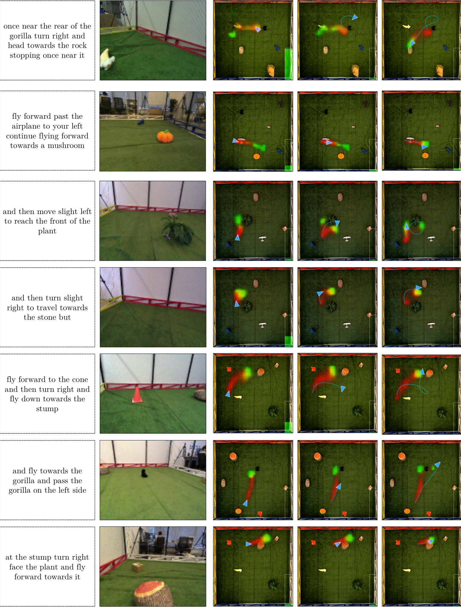
Visualization of Intermediate Representations
Figure 8 shows the intermediate representations and visitation predictions over time during instruction execution for the examples used in Figures 2-3, illustrating the model reasoning. The model is able to output the action to stop on the right side of the banana, even after the banana has disappeared from the first-person view. This demonstrates the advantages of using an explicit spatial map aggregated over time instead, for example, a learned hidden state vector representing the agent state.

Appendix B Model Details
B.1 Stage 1: Visitation Distribution Prediction
The first-stage model is largely based on the Position Visitation Network, except for several improvements we introduce:
- •
Computing observability and boundary masks and that are used to track unexplored space and environment boundaries.
- •
Introducing a placeholder position that represents all unobserved positions in the environment for use in the visitation distributions.
- •
Modification to the LingUNet architecture to support outputting a probability score for the unobserved placeholder position, in addition to the 2D distributions over environment positions.
- •
Predicting 2D probability distributions only over observed locations in the environment.
- •
Minor hyperparameter changes to better support the longer instructions.
The description in Section B.1 has been taken from Blukis et al. 2018. We present it here for reference and completeness, with minor modifications to highlight technical differences.
B.1.1 Instruction Representation
We represent the instruction as an embedded vector . We generate a series of hidden states , , where LSTM is a Long-Short Term Memory recurrent neural network (RNN) and is a learned word-embedding function. The instruction embedding is the last hidden state . This part is replicated as is from Blukis et al. 2018.
B.1.2 Semantic Mapping

We construct the semantic map using the method of Blukis et al. 2018. The full details of the process are specified in the original paper. Roughly speaking, the semantic mapping process includes three steps: feature extraction, projection, and accumulation. At timestep , we process the currently observed image using a 13-layer residual neural network CNN (Figure 9) to generate a feature map of size . We compute a feature map in the world coordinate frame by projecting with a pinhole camera model onto the ground plane at elevation zero.
The semantic map of the environment at time is an integration of and , the map from the previous timestep. The integration equation is given in Section 4c in Blukis et al. 2018. This process generates a tensor of size that represents a map, where each location is a -dimensional feature vector computed from all past observations , each processed to learned features and projected onto the environment ground in the world frame at coordinates . This map maintains a learned high-level representation for every world location that has been visible in any of the previously observed images. We define the world coordinate frame using the agent starting pose ; the agent start position is the coordinates , and the positive direction of the -axis is along the agent heading. This gives consistent meaning to spatial language, such as turn left or pass on the left side of.
B.1.3 Grounding
We create the grounding map with a 11 convolution . The kernel is computed using a learned linear transformation , where is the instruction embedding. The grounding map has the same height and width as , and during training we optimize the parameters so it captures the objects mentioned in the instruction (Section C.4).
B.1.4 LingUNet and Visitation Distributions

The following paragraphs are adapted from Blukis et al. 2018 and formally define the LingUNet architecture with our modifications. Figure 10 illustrates the architecture.
LingUNet uses a series of convolution and scaling operations. The input map is processed through cascaded convolutional layers to generate a sequence of feature maps , .11 1 denotes concatenation along the channel dimension. Each is filtered with a 11 convolution with weights . The kernels are computed from the instruction embedding using a learned linear transformation . This generates language-conditioned feature maps , . A series of upscale and convolution operations computes feature maps of increasing size:
We modify the original LingUNet design by adding an output head that outputs a vector h:
where AvgPool takes averages across the dimensions.
The output of LingUNet is a tuple (, h), where is of size and h is a vector of length 2. This output is used to compute two distributions, and can be increased if more distribution are predicted, such as in Suhr et al. 2019. We use an additional normalization step to produce the position visitation and goal visitation distributions given (, h).
B.2 Control Network: Action Generation and Value Function
Figure 11 shows the architecture of the control network for the second action generation stage of the model. The value function architecture is identical to the action generator and also uses the control network, except that it has only a single output. The value function does not share the parameters with the action generator.
The control network takes as input the trajectory and stopping visitation distributions and , as well as the observability and boundary masks and . The distributions and are represented as 2D square-shaped images over environment locations, where unobserved locations have a probability of zero. Additional scalars and define the probability mass outside of any observed environment location.
The visitation distributions and are first rotated to the agent’s current ego-centric reference frame, concatenated along the channel dimension, and then processed with a convolutional neural network. The output is flattened into a vector. The masks and are processed in an analogous way to the visitation distributions and , and the output is also flattened into a vector. The scalars and are embedded into fixed-length vectors:
where are random fixed-length vectors. We do not tune .
The resulting vector representations for the visitation distributions, out-of-bounds probabilities, and masks are concatenated and processed with a three-layer multi-layer perceptron (MLP). The output are five scalars. Two of the scalars are predicted forward and angular velocities and , one scalar is the logit of the stopping probability, and two scalars are standard deviations used during PPO training to define a Gaussian probability distribution over actions.
B.3 Coordinate Frames of Reference
At the start of each task, we define the world reference frame according to the agent’s starting position, with x and y axis pointing forward and left respectively, according to the agent’s position. The maps are represented with the origin at the center. Throughout the instruction execution, this reference frame remains fixed. Within the first model stage, the semantic and grounding maps, observability and boundary masks, and visitation distributions are all represented in the world reference frame. At the input to second stage, we transform the visitation distributions, and observability and boundary masks to the agent’s current egocentric frame of reference. This allows the model to focus on generating velocities to follow the high probability regions, without having to reason about coordinate transformations.
Appendix C Additional Learning Details
C.1 Discriminator Architecture and Training
Figure 12 shows the neural network architecture of our discriminator . The Wasserstein distance estimation procedure from Shen et al. 2018 requires a discriminator that is K-Lipschitz continuous. We guarantee that our discriminator meets this requirement by clamping the discriminator parameters to a range of after every gradient update [40].
C.2 Return Definition
The expected return is defined as:
where is a policy execution, is the agent context observed at state , is a discount factor, and is the intrinsic reward. The reward does not depend on any external state information, but only on the agent context and visitation predictions.
C.3 Reward Function
Section 5 provides the high level description and motivation of the intrinsic reward function.
Visitation Reward
We design the visitation reward to reward policy executions that closely match the predicted visitation distribution . An obvious choice would be the probability of the trajectory under independence assumptions . According to this measurement, if for any , then . This would lead to a reward of zero as soon as the policy makes a mistake, resulting in sparse rewards and slow learning. Instead, we define the visitation reward in terms of earth mover’s distance that provides a smooth and dense reward. The visitation reward is:
where is a reward shaping potential:
EMD is the earth mover’s distance in Euclidean space, is a probability distribution that assigns equal probability to all positions visited thus far, is the set of positions the agent has observed so far,22 2 We restrict the metric to observed locations on the map, because as discussed in Section 4, all unobserved locations are represented by a dummy location . and is the position visitation distribution over all observed positions. Intuitively, rewards per-timestep reduction in earth mover’s distance between the predicted visitation distribution and the empirical distribution derived from the agent’s trajectory.
Stop Reward
Similar to , the stop reward is the negative earth mover’s distance between the conditional predicted goal distribution over all observed environment locations, and the empirical stop distribution that assigns unit probability to the agent’s final stopping position.
Exploration Reward
The exploration reward is:
| (3) |
where:
The term reflects the agent’s belief that it has observed the goal location . is the probability that the goal has been observed before time . We take the maximum over past timesteps to reduce effects of noise from the model output. The second term in Equation 3 penalizes the agent for stopping while it predicts that the goal is not yet observed.
C.4 Auxiliary Objectives
During training, we add an additional auxiliary loss to the supervised learning loss to ensure that the different modules in the PVN model specialize according to their function. The auxiliary loss is:
| (4) |
The text in the remainder of Section C.4 has been taken from Blukis et al. 2018. We present it here for reference and completeness.
Object Recognition Loss
The object-recognition loss ensures the semantic map stores information about locations and identities of objects. At timestep , for every object that is visible in the first person image , we classify the feature vector in the position in the semantic map corresponding to the object location in the world. We use a linear softmax classifier to predict the object identity given the feature vector. At a given timestep the classifier loss is:
where is the true class label of the object and is the predicted probability. is the set of objects visible in the image .
Grounding Loss
For every object visible in the first-person image , we use the feature vector from the grounding map corresponding to the object location in the world with a linear softmax classifier to predict whether the object was mentioned in the instruction . The objective is:
where is a 0/1-valued label indicating whether the object o was mentioned in the instruction and is the corresponding model prediction. is the set of objects visible in the image .
Language Loss
The instruction-mention auxiliary objective uses a similar classifier to the grounding loss. Given the instruction embedding , we predict for each of the possible objects whether it was mentioned in the instruction . The objective is:
where is a 0/1-valued label, same as above.
Automatic Word-object Alignment Extraction
In order to infer whether an object was mentioned in the instruction , we use automatically extracted word-object alignments from the dataset. Let be the event that an object occurs within 15 meters of the human-demonstration trajectory , let be the event that a word type occurs in the instruction , and let be the event that both and occur simultaneously. The pointwise mutual information between events and over the training set is:
where the probabilities are estimated from counts over training examples . The output set of word-object alignments is:
where and are threshold hyperparameters.
Appendix D Dataset Details
| Dataset | Type | Split | # Paragraphs | # Instr. | Avg. Instr. Len. (tokens) | Avg. Path Len. (m) |
|---|---|---|---|---|---|---|
| Lani | 1-segment | Train | 4200 | 19762 | 11.04 | 1.53 |
| Dev | 898 | 4182 | 10.94 | 1.54 | ||
| Test | 902 | 4260 | 11.23 | 1.53 | ||
| [0.5pt/1pt] | 2-segment | Train | 4200 | 15919 | 21.84 | 3.07 |
| Dev | 898 | 3366 | 21.65 | 3.10 | ||
| Test | 902 | 3432 | 22.26 | 3.07 | ||
| Real | 1-segment | Train | 698 | 3245 | 11.10 | 1.00 |
| Dev | 150 | 640 | 11.47 | 1.06 | ||
| Test | 149 | 672 | 11.31 | 1.06 | ||
| [0.5pt/1pt] | 2-segment | Train | 698 | 2582 | 20.97 | 1.91 |
| Dev | 150 | 501 | 21.42 | 2.01 | ||
| Test | 149 | 531 | 21.28 | 1.99 |
Natural Language and Demonstration Data
Table 2 provides statistics on the natural language instruction datasets.
Lani Dataset Collection Details
The crowdsourcing process includes two stages. First, a Mechanical Turk worker is shown a long, random trajectory in the overhead view and writes an instruction paragraph for a first-person agent. The trajectories were generated with a sampling process biased towards moving around the landmarks. Given the instruction paragraph, a second worker follows the instructions by controlling a discrete simple agent, simultaneously segmenting the instruction and trajectory into shorter segments. The output are pairs of instruction segments and discrete ground-truth trajectories. We restrict to a pool of workers who had previously qualified for our other instruction-writing tasks.
Demonstration Data
We collect the demonstration datasets and by executing a hand-engineered oracle policy that has access to the ground truth human demonstrations, and collect observation data. The oracle is described in Appendix E.2. includes all instructions from original Lani data, as well as the additional instructions we collect for our smaller environment. Due to the high cost of data collection on the physical quadcopter, includes demonstrations on only 100 paragraphs of single-segment instructions, approximately 1.5% of the data available in simulation.
Data Augmentation
To improve generalization, we perform two types of data augmentation. First, we train on the combined dataset that includes both single-segment and two-segment instructions. Two-segment data consists of instructions and executions that combine two consecutive segments. This increases the mean instruction length from 11.10 tokens to 20.97, and the mean trajectory length by a factor of 1.91. Second, we randomly rotate the semantic map and the gold visitation distributions by a random angle to counter the bias of always flying forward, which is especially present in the single-segment data because of how humans segmented the original paragraphs.
Appendix E Additional Experimental Setup Details
E.1 Computing hardware and training time
Training took approximately three days on an Intel i9 7980X CPU with three Nvidia 1080Ti GPUs. We used one GPU for the supervised learning process, one GPU for the RL process for both gradient updates and roll-outs, and one GPU for rendering simulator visuals. We ran five simulator processes in parallel, each at 7x real-time speed. We used a total of 400k RL simulation rollouts.
E.2 Oracle implementation
The oracle uses the ground truth trajectory, and follows it with a control rule. It adjusts its angular velocity with a P-control rule to fly towards a dynamic goal on the ground truth trajectory. The dynamic goal is always 0.5m in front of the quadcopter’s current position on the trajectory, until it overlaps the goal position. The forward speed is a constant maximum minus a multiple of angular velocity.
E.3 Environment and Quadcopter Parameters
Environment Scaling
The original Lani dataset includes a unique 50x50m environment for each paragraph. Each environment includes 6–13 landmarks. Because the original data is for a larger environment, we scale it down to the same dimension as ours. We use the original data split, where environments are not shared between the splits.
Action Range
We clip the forward velocity to the range m/s and the yaw rate to rad/s. During training, we give a small negative reward for sampling an action outside the intervals m/s for forward velocity and rad/s for yaw-rate. This reduces the chance of action predictions diverging, and empirically ensures they stay mostly within the permitted range.
Quadcopter Safety
We prevent the quadcopter from crashing into environment bounds through a safety interface that modifies the controller setpoint . The safety mechanism performs a forward-simulation for one second and checks whether setting as the setpoint would cause a collision. If it would, the forward velocity is reduced, possibly to standstill, until it would no longer pose a threat. Angular velocity is left unmodified. This mechanism is only used when collecting demonstration trajectories and during test-time. No autonomous flight in the physical environment is done during learning.
First-person Camera
We use a front-facing camera on the Intel Aero drone, tilted at a 15 degree pitch. The camera has a horizontal field-of-view of 84 degrees, which is less than the 90-degree horizontal FOV of the camera used in simulated experiments of Blukis et al. 2018.
Appendix F Evaluation Details
F.1 Automated Evaluation Details
We report two automated metrics: success rate and earth mover’s distance (EMD). The success rate is the frequency of executions in which the quadcopter stopped within 0.47m of the human demonstration stopping location. To compute EMD, we convert the trajectories executed by the quadcopter and the human demonstration trajectories to probability distributions with uniformly distributed mass across all positions on the trajectory. EMD is then the earth mover’s distance between these two distributions, using Euclidean distance as the distance metric. EMD has a number of favorable properties, including: (a) taking into account the entire trajectory and not only the goal location, (b) giving partial credit for trajectories that are very close but do not overlap the human demonstrations, and (c) is smooth in that a slight change in the executed trajectory corresponds to at most a slight change in the metric.
F.2 Human Evaluation Details
Navigation Instruction Quality
One out of 73 navigation instructions that the majority of workers identified as unclear is excluded from the human evaluation analysis. The remaining instructions were judged by majority of workers not to contain mistakes, or issues with clarity or feasibility.
We need your help to understand how well our drone follows instructions. Your task: Read the navigation instruction below, and watch the animation of the drone trying to follow the instruction. Then answer three questions. Consider the guidelines below: • Looking around: The drone can only see what’s directly in front of it as indicated by the highlighted region. Depending on the instruction, it may have to look for certain objects to understand where to go, and looking around for them is the right way to go and is efficient. • Bad instructions: If the instruction is unclear, impossible, or full of confusing mistakes, please indicate it by checking the checkbox. You must still answer all the questions - consider if the drone’s behavior was reasonable given the bad instruction. • Objects: The drone observes the environment from a first-person view. The numbered images illustrate how each object would look like to the drone. Consider the appearance of objects from the first-person perspective in relation to the instructions. • Note: Try to answer each question in isolation, focusing on the specific behavior. For example, if the drone reached the goal correctly, but took the wrong path, you should answer "Yes, perfectly" for question 2, while giving a worse score for question 1. Similarly, if the drone went straight for the goal, that would be considered "efficient" behavior, even though it may have taken the wrong path to get there • The drone might sometimes decide not to do anything at all, maybe because it thinks it’s already where it was instructed to go. If that happens you won’t see any movement in the animation. • The drone always "stops" at the end, even if the motion appears to end abruptly. • The field is surrounded by a red fence on top, white fence on the right, blue fence on the bottom, and yellow fence on the left. The colorful borders are there to help you better distinguish between these colors.
Mechanical Turk Evaluation Task
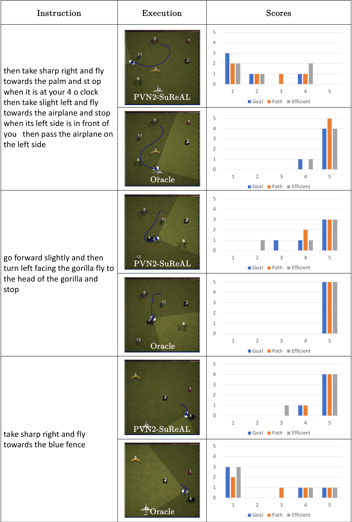
Figure 13 shows the instructions given to workers for the human evaluation task. Figure 14 shows an example human evaluation task. We use the simulated environment to visualize the quadcopter behavior to the workers because it is usually simpler to observe. However, we use this interface to evaluate performance on the physical environment, and use trajectories generated in the physical environment. We avoid using language descriptions to describe objects to avoid biasing the workers, and allowing them to judge for themselves how well the instruction matches the objects. We observed that a large number of workers were not able to reliably judge the efficiency of agent behavior, since they generally considered correct behavior efficient and incorrect behavior inefficient. Therefore, we do not report efficiency scores. Figure 15 shows examples of human judgements for different instruction executions.

Appendix G Additional Results
Table 3 shows simulation results on the full Lani test and development data.
| Method | 1-segment | 2-segment | ||
| SR | EMD | SR | EMD | |
| Test Results On Full Lani Test Set | ||||
| Stop | 7.7 | 0.76 | 0.7 | 1.29 |
| Average | 13.0 | 0.62 | 5.8 | 0.94 |
| [0.5pt/1pt] PVN-BC | 37.8 | 0.47 | 19.6 | 0.76 |
| PVN2-BC | 39.0 | 0.43 | 21.0 | 0.72 |
| PVN2-SuReAL | 37.2 | 0.43 | 21.5 | 0.67 |
| [0.5pt/1pt] Oracle | 98.6 | 0.15 | 93.9 | 0.20 |
| Dev Results On Full Lani Test Set | ||||
| PVN2-SuReAL | 35.8 | 0.44 | 19.8 | 0.68 |
| PVN2-SuReAL-noExp | 38.5 | 0.43 | 15.8 | 0.79 |
| PVN2-SuReAL-noU | 26.1 | 0.48 | 7.0 | 0.90 |
Appendix H Common Questions
Do you assume any alignment between simulated and real environments?
Our learning approach does not assume that simulated and real data is aligned.
What is the benefit of SuReAL over reinforcement learning with an auxiliary loss as a means of utilizing annotated data?
There are a number of reasons to prefer SuReAL:
- •
The 2-stage decomposition means that there is no gradient flow from second to first stage, and so the policy gradient loss will not update Stage 1 parameters anyway.
- •
With SuReAL, only the second stage needs to be computed during the PPO updates, which drastically improves training speed.
- •
In SuReAL, we do not need to send new Stage 1 parameters to actor processes at every iteration, since these parameters are not optimized with reinforcement learning.
Why did you select this particular set of baselines?
The baselines have been developed for instruction following in a very similar environment to ours, allowing us to focus on evaluating domain transfer performance, exploration performance, and the effect of our learning method. Instruction-following tasks have unique requirements for sample complexity and utilizing limited annotated data. Comparisons against general sim-to-real models may not yield useful insights, or yield insights that have already been demonstrated in prior work [34].
Why do you learn control, rather than using deterministic control?
The predicted visitation distributions often have complex and unpredictable shapes, depending on the instruction and environment layout. Designing a hand-engineered controller that effectively follows the predicted distributions reduces to either (a) a challenging optimal control problem at test time or (b) a difficult engineering and testing challenge. We instead opt to learn a solution at training time. We find that learning Stage 2 behavior is more straightforward, and is in line with our general strategy of reducing engineering effort and use of hand-crafted representations.
How noisy are your pose estimates?
We use a Vicon motion capture system to obtain pose estimates. The poses have sub-centimeter positional accuracy, but often arrive at the drone with delay due to network latency.
Is the model tolerant to noise?
Prior work has tested the semantic mapping module that we use against noisy poses and found that it can tolerate moderate amounts of noise [34] even without explicit probabilistic modelling. This is not the focus of this paper, but we find that our model is able to recover from erroneous pose-image pairs caused by network latency. Evaluating the robustness of the model to more types of noise, including in pose estimates, is an important direction for future work.
Appendix I Hyperparameters
Table 4 shows the hyperparameter assignments. The hyperparameters were manually tuned on the development set to trade off use of computational resources and development time. We do not claim the selected hyperparameters are optimal, but we did observe that they consistently resulted in learning convergence and stable test-time behavior.
| Hyperparameter | Value |
| Environment Settings | |
| Maximum yaw rate | |
| Maximum forward velocity | |
| Image and Feature Dimensions | |
| Camera horizontal FOV | |
| Input image dimensions | |
| Feature map dimensions | |
| Semantic map dimensions | |
| Visitation distributions and dimensions | |
| Environment edge length in meters | |
| Environment edge length in pixels on | |
| Model | |
| Visitation prediction interval timesteps | |
| action threshold | |
| General Learning | |
| Deep Learning library | PyTorch 1.0.1 |
| Classification auxiliary weight | |
| Grounding auxiliary weight | |
| Language auxiliary weight | |
| Supervised Learning | |
| Optimizer | ADAM |
| Learning Rate | |
| Weight Decay | |
| Batch Size | |
| Reinforcement Learning (PPO) | |
| Num supervised epochs before starting RL () | 25 |
| Num epochs () | 400 |
| Iterations per epoch ( | 50 |
| Number of parallel actors | 4 |
| Number of rollouts per iteration | 20 |
| PPO clipping parameter | 0.1 |
| PPO gradient updates per iter ( | 8 |
| Minibatch size | 2 |
| Value loss weight | 1.0 |
| Learning rate | 0.00025 |
| Epsilon | 1e-5 |
| Max gradient norm | 1.0 |
| Use generalized advantage estimation | False |
| Discount factor () | 0.99 |
| Entropy coefficient | 0.001 |
| Entropy schedule | multiply entropy coefficient by 0.1 after 200 epochs |
| Reward Weights | |
| Stop reward weight () | 0.5 |
| Visitation reward weight() | 0.3 |
| Exploration reward weight () | 1.0 |
| Negative per-step reward () | -0.04 |