The chemical composition of the Herbig Ae SB2 system AK Sco (HD 152404) 2019The chemical composition of the Herbig Ae SB2 system AK Sco (HD 152404)–1
Abstract
We investigate the stellar atmospheres of the two components of the Herbig Ae SB2 system AK Sco to determine the elements present in the stars and their abundance. Equal stellar parameters K and were used for both stars. We studied HARPSpol spectra (resolution 110 000) that were previously used to state the presence of a weak magnetic field in the secondary. A composite synthetic spectrum was compared in the whole observed region 3900–6912 Å with the observed spectrum. The abundances were derived mostly from unblended profiles, in spite of their sparsity, owing to the complexity of the system and to the not negligible of 18 km s-1 and 21 km s-1 adopted for the two components, respectively. The identified elements are those typical of stars with spectral type F 5 IV-V, except for Li i at 6707 Å and He i at 5875.61 Å, whose presence is related with the Herbig nature of the two stars. Furthermore, overabundances were determined in both stars for Y, Ba, and La. Zirconium is overabundant only in the primary, while sulfur is overabundant outside the adopted error limits only in the secondary. In contrast to previous results showing a high occurrence rate of Boo peculiarities or normal chemical composition among the Herbig Ae/Be stars, the abundance pattern of AK Sco is similar to that of only few other Herbig stars displaying weak Ap/Bp peculiarities. A few accretion diagnostic lines are discussed.
Keywords:
line: identification – atomic data – stars: atmospheres – stars: chemically peculiar – stars: individual: AK Sco1 Introduction
The combination of knowledge about the magnetic field structure and the determination of the stellar chemical composition is very likely the key to constrain theories on star formation and magnetospheric accretion in intermediate-mass Herbig Ae/Be stars. These stars are surrounded by active accretion disks and most of the excess emission present at various wavelengths can probably be ascribed to the interaction of the disk with a magnetically active star (e.g. Muzerolle et al. 2004).
Magnetic Herbig Ae/Be stars are frequently considered as precursors of the magnetic Ap stars (e.g. Stepień & Landstreet 2002; Catala 2003). However, in contrast to chemical peculiar magnetic Ap stars, for which the abundance anomalies are believed to be produced by mechanisms intrinsic to the stars themselves, such as radiatively driven diffusion (e.g. Michaud 1970), the photospheric material in Herbig Ae/Be stars is mixed with circumstellar material originating in a protoplanetary disk. Therefore, studies of photospheric composition in these stars can also provide information on protoplanetary material.
Only very few abundance analyses of Herbig Ae/Be stars were carried out in the past. Cowley et al. 2010 reported on a chemical composition similar to that in Boo stars in the magnetic Herbig Ae star HD 101412. Later-on, Folsom et al. 2012 reported on the abundance analysis of 20 Herbig Ae/Be stars, concluding that half the stars in their sample show Boo chemical peculiarities. Only one star in their study showed weak Ap/Bp peculiarities and all the remaining stars were chemically normal. In contrast, the abundance study of the double-lined spectroscopic binary (SB2) system HD 104237 by Cowley, Castelli & Hubrig 2013 showed slight enhancements of a few elements, where the case for Zr was the strongest. The Herbig Ae star PDS 2 was studied by Cowley, Hubrig & Przybilla 2014 and found to have Boo characteristics.
AK Sco (HD 152404) is a double-lined spectroscopic binary system formed by two nearly identical Herbig Ae stars (F5 V spectral type) surrounded by a circumbinary disk. Furthermore, the gap between the stars and the disk is filled by some gas. The Herbig nature of AK Sco was first stated by Herbig & Kameswara Rao 1972, who observed H emission with a deep reversal and Li i absorption at 6707 Å in Coudé spectrograms. However, according to Andersen et al. 1989, a follow-up observation with the ESO 1.5 m telescope on La Silla in 1986 did not reveal the presence of emission lines in the blue spectral region. On the other hand, this observation showed doubling of all photospheric spectroscopic lines, indicating that AK Sco is a spectroscopic binary with approximately equal components. Subsequent radial-velocity observations discovered that it is indeed a SB2 system with a short period (13.6 days) and large eccentricity () (Andersen et al. 1989).
Alencar et al. 2003 reconsidered the orbital parameters and the physical elements of the system finding a substantial agreement with the results of Andersen et al. 1989. Furthermore, Alencar et al. 2003 inferred the pre-main-sequence (PMS) nature of the secondary from the presence of the strong Li i line at 6707 Å in the spectrum. A characteristic of AK Sco is the light variability, which was shown to be related to a variable circumstellar obscuration (Andersen et al. 1989; Alencar et al. 2003) rather than to the orbital motion of the two components. Recent spectropolarimetric observations using HARPSpol spectra, performed at six different orbital phases (, 0.950, 0.018, 0.025, 0.090, and 0.169), indicated the presence of a weak magnetic field of the order of 80 G in the secondary component at the phase 0.090 (Järvinen et al. 2018). This discovery raised the question whether chemical peculiarities like those observed in the main sequence Ap stars can be observed also in AK Sco.
There are only few studies on the chemical composition of magnetic Herbig Ae/Be stars. Folsom et al. 2012 analyzed the abundances in a sample of 21 Herbig Ae/Be stars. Three of them are affected by the presence of a magnetic field. They found that the magnetic Herbig stars do not exhibit a chemical composition remarkably different from the normal stars. One of them (HD 101412) displays Boo chemical peculiarities, another (V 380 Ori A) shows weak Ap/Bp peculiarities, and the third one (HD 190073) was found to be normal. The chemical composition of HD 101412 and HD 190073 was also studied by Cowley et al. 2010 and Cowley & Hubrig 2012, respectively. Their results roughly agree with those from Folsom et al. 2012. In addition, Cowley, Castelli & Hubrig 2013 and Cowley, Hubrig & Przybilla 2014 analyzed the spectra of two other magnetic Herbig Ae stars, HD 104237 and PDS2. The presence of a magnetic field was dubious for PDS2, until Hubrig et al. 2015 definitively detected it.
Abundances for fourteen magnetic (including HD 104237) and non-magnetic Herbig Ae/Be stars were also presented by Acke & Waelkens 2004. Both Cowley, Castelli & Hubrig 2013 and Acke & Waelkens 2004 demonstrated that the abundances of HD 104237 are slightly peculiar with enhanced elements Y, Zr, Ba, and La. The agreement between the results from the two studies concerning these elements is within 0.07 dex. In contrast, the chemical composition of PDS2 was found to be similar to that of the Boo stars.
In this paper we use HARPSpol spectra covering the 3900–6912 Å region to investigate the composite spectrum of AK Sco with the aim to increase the number of abundance analyses of magnetic Herbig Ae/Be stars.
2 Observations

We used the same HARPSpol spectropolarimetric observations of AK Sco and the same reduced spectra that are described in Järvinen et al. 2018. Here we recall that the observations cover six orbital phases (0.946, 0.950, 0.018, 0.025, 0.090, 0.169) of the binary system. The covered orbital phases (calculated using the orbital solution from Alencar et al. 2003 are presented in Fig. 1. While the observed wavelength interval is 37806912 Å, with a small gap between 5259 and 5337 Å, the region useful for the analysis starts at 3900 Å because the noise is too strong at lower wavelengths. The resolving power is about 110 000.
In this work, the normalization to the continuum performed by Järvinen et al. 2018 was adjusted at intervals of 6 Å by comparing observed and computed spectra. The continuum level was lowered from about 30% at 4000 Å, to about 5% at 4600 Å, to 0.050.25% for 5000 Å. In all the spectra, except for that at the phase 0.169, the spectral lines of both components are well separated. The variability was studied by using all six spectra observed at the different epochs.
3 Stellar parameters and synthetic spectra
| Date | Phase | (B)-(A) | (A) | ||
|---|---|---|---|---|---|
| [km s-1] | [km s-1] | [%] | |||
| 1 | 2016-06-15 | 0.946 | 138 | 70 | 10 |
| 2 | 2017-06-04 | 0.950 | 146 | 72.5 | 50 |
| 3 | 2016-06-18 | 0.018 | 180 | 90 | 50 |
| 4 | 2017-06-05 | 0.025 | 177 | 87 | 80 |
| 5 | 2017-06-06 | 0.090 | 74 | 36 | 100 |
| 6 | 2017-06-07 | 0.169 | 1. | 0. | 100 |
The abundances were derived from the spectrum observed at the phase , i.e. from the spectrum for which the presence of a weak magnetic field was established (Järvinen et al. 2018). Furthermore, at this phase the two stars are well separated with a radial velocity shift km s-1 (see Table 1).
The double-line spectrum, the similar intensity of the lines from the two stars, and the rather high rotational velocities (18 km s-1 and 21 km s-1, respectively) increase the number of blended profiles, so that it is very difficult to pick up lines that do not have any contamination with lines either from the same star or from the companion. Therefore, the whole analysis was performed with the synthetic spectrum method. Unblended lines are rare, so that the abundance for a given element was determined from the profiles of few single lines, when available. Then the abundance was checked on blended lines having the element as main or sometimes even minor component of the blend.
The atomic and molecular line lists adopted to compute the synthetic spectra were produced by Castelli22 2 http://wwwuser.oats.inaf.it/castelli/linelists.html, who assembled the line lists from the GFNEW directory (Kurucz 2018), available at the Kurucz website33 3 http://kurucz.harvard.edu/linelists.html, with line lists taken from the literature for some ions missing in the Kurucz data. Furthermore, if needed, the values in the Kurucz line lists were replaced by values either extracted from various literature sources or obtained by fitting the solar synthetic spectrum to the observed solar flux Atlas from Kurucz 2005a. For numerous lines, Van der Waals broadening was computed according to the Anstee & O’Mara 1995 theory. The and parameters were taken from the Barklem, Piskunov & O’Mara 2000 tables.
We adopted for both stars K from Andersen et al. 1989, who inferred this temperature on the basis of the F5 V spectral type. They used the spectral type calibration given by Bessell 1979 and by Popper 1980. For this value of , Alencar et al. 2003 determined the system parameters assuming nearly identical components, in particular M⊙, R⊙, and km s-1, provided that the stellar inclination is between 65 and 70 degrees. The gravity, deduced from the mass and radius given above, is .

In order to check the gravity obtained from mass and radius spectroscopically, we used the wings of the Mg i triplet at 5167.321, 5172.684, and especially 5183.604 Å, because it does not show the slight redshift as the other two lines do. At first, we determined the Mg abundance for K and using the Mg ii line at 4481 Å, which is almost independent of gravity. For this abundance and the computed wings of the Mg i triplet were too narrow. To improve the agreement between the observed and computed Mg i profiles we increased the gravity to (Fig. 2). We note that when the line data were checked on the solar spectrum, we decreased for the Mg i triplet the parameter from , as given by Barklem, Piskunov & O’Mara 2000, to . Probably, a different solar model than that used by us would have given good agreement between observed and computed wings of the solar Mg i triplet for . For the Sun, we adopted an ATLAS9 model with parameters K and , and turbulent velocity km s-1. This model was used because it is consistent with the ATLAS9 model adopted to analyze AK Sco.
An ATLAS9 model atmosphere with parameters K and from the updated Castelli & Kurucz 200444 4 http://wwwuser.oats.inaf.it/castelli/grids.html grid was used to compute synthetic spectra for both components by means of the SYNTHE code (Kurucz 2005b). On the basis of the comparison of the observed and computed profiles, the microturbulent velocity was estimated to be km s-1 and km s-1 for the primary and the secondary, respectively. The rotational velocity was determined from the comparison of observed and computed profiles of numerous stellar features (e.g. Mg ii 4481 Å). We adopted the values 18 km s-1 and 21 km s-1 for the primary and the secondary, respectively. Finally, the computed profiles were broadened for a Gaussian instrumental profile, corresponding to the resolving power 110 000 of the HARPSpol spectrum.
The composite spectrum was obtained with the BINARY code (Kurucz 1995). As described by Cowley, Castelli & Hubrig 2013, the spectra of the two components are shifted in respect to each other in accordance with the observed radial velocity difference. Then, they were weighted with the luminosity ratio and added together. The adopted luminosity ratio is 1.0, corresponding to a radii ratio equal to 1.0 (Gómez de Castro 2009). Because not only all the accretion diagnostic lines, but also photospheric lines show intensity variations over the observing nights (Järvinen et al. 2018), we investigated whether the photospheric line variability may be caused by abundance changes. By comparing observed and computed spectra at different phases, we concluded that the variability of the photospheric lines should be mostly related to the presence of the circumbinary disk, which obscures the secondary component with dust clouds with different densities at different phases. We assumed “a priori” that there is no obscuration at the phase 0.090, so that we adopted as stellar abundances those derived at this phase. For the other phases, we determined for the secondary the fraction in percent of the observed luminosity to its total luminosity on the basis of the Li i profile at 6707 Å. We assumed that the abundance of Li i in all phases is the same as that at the phase 0.090. Table 1 summarizes for the different phases the radial velocity difference for the two stars, the radial velocity of the primary as determined from the spectra, and the observed luminosity fraction (in %) of the secondary.
4 Identification and abundances
| Element | A component | B component | Sun | ||
|---|---|---|---|---|---|
| ( K, ) | ( K, ) | ||||
| Li i | 8.70 (1) | [+2.29] | 8.50 (1) | [+2.49] | 10.99 |
| C i | 3.61 (1) | [0.00] | 3.61 (1) | [0.00] | 3.61 |
| O i | 3.35 (3) | [0.00] | 3.35 (3) | [0.00] | 3.35 |
| Na i | 5.93 (2) | [0.10] | 5.780.05 (3) | [+0.05] | 5.83 |
| Mg i | 4.55 (2) | [0.10] | 4.45 (3) | [+0.00] | 4.45 |
| Mg ii | 4.55 (1) | [0.10] | 4.45 (1) | [+0.00] | 4.45 |
| Al i | 5.61 (2) | [0.00] | 5.61 (2) | [+0.00] | 5.61 |
| Si i | 4.400.07 (12) | [+0.13] | 4.310.06 (7) | [+0.22] | 4.53 |
| Si ii | 4.40 (1) | [+0.13] | 4.40 (1) | [+0.13] | 4.53 |
| Sitot | 4.400.07 | [+0.13] | 4.330.07 | [+0.20] | 4.53 |
| S i | 4.720.10 (2) | [+0.20] | 4.620.10 (2) | [+0.30] | 4.92 |
| Ca i | 5.700.10 (15) | [+0.02] | 5.840.08 (12) | [0.12] | 5.72 |
| Sc ii | 8.98 (3) | [0.10] | 8.68 (2) | [+0.20] | 8.88 |
| Ti i | 7.140.04 (3) | [0.03] | 7.11 | ||
| Ti ii | 6.880.09 (6) | [+0.23] | 7.140.09 (3) | [0.03] | 7.11 |
| Titot | 6.960.15 | [+0.15] | 7.140.09 | [0.03] | 7.11 |
| V i | 8.15 (2) | [0.00] | 8.15 | ||
| Cr i | 6.410.12 (4) | [+0.01] | 6.42 (3) | [0.00] | 6.42 |
| Cr ii | 6.220.20 (2) | [+0.20] | 6.350.04 (3) | [+0.07] | 6.42 |
| Crtot | 6.340.17 | [+0.08] | 6.390.02 | [+0.03] | 6.42 |
| Mn i | 6.62 (3) | [0.00] | 6.62 (2) | [0.00] | 6.62 |
| Fe i | 4.660.15 (12) | [0.11] | 4.510.17 (11) | [+0.06] | 4.57 |
| Fe ii | 4.42 (2) | [+0.15] | 4.440.06 (5) | [+0.13] | 4.57 |
| Fetot | 4.620.16 | [0.05] | 4.490.15 | [+0.08] | 4.57 |
| Co i | 6.91 (1) | [+0.20] | 7.11 | ||
| Ni i | 5.840.08 (9) | [0.00] | 5.740.17 (8) | [+0.14] | 5.84 |
| Cu i | 7.86 (1) | [0.00] | 7.86 (1) | [+0.00] | 7.86 |
| Zn i | 7.38 (2) | [+0.10] | 7.58 (2) | [0.10] | 7.48 |
| Sr i | 9.00 (1) | [+0.21] | 9.21 | ||
| Sr ii | 9.10 (1) | [+0.11] | 8.90 (1) | [+0.29] | 9.21 |
| Srtot | 9.10 | [+0.11] | 8.950.05 | [+0.24] | 9.21 |
| Y ii | 9.40 (2) | [+0.40] | 9.50 (1) | [+0.30] | 9.83 |
| Zr ii | 9.05 (2) | [+0.40] | 9.45 (1) | [0.00] | 9.45 |
| Ba ii | 9.51 (1) | [+0.28] | 9.41 (1) | [+0.38] | 9.79 |
| La ii | 10.220.15 (2) | [+0.71] | 10.57 (1) | [+0.36] | 10.93 |
| Ce ii | 10.46 (1) | [+0.00] | 10.46 | ||
| Nd ii | 10.62 (1) | [+0.00] | 10.62 | [+0.00] | 10.62 |
The whole available spectrum from 3900 Å to 6900 Å was synthetized and compared with the HARPSpol spectrum. In order to derive the abundances, we analyzed the profiles of the lines listed in the Appendix. The comparison of the observed spectrum with the spectrum computed with the final abundances listed in Table 2 is available from Castelli’s webpage55 5 http://wwwuser.oats.inaf.it/castelli/stars/AK_Sco/ AK_Sco.html. We identified in both stars: H i, Li i, C i, O i, Na i, Mg i, Mg ii, Al i, Si i, Si ii, S i, Ca i, Ca ii, Sc i, Sc ii, Ti i, Ti ii, V i, V ii, Cr i, Cr ii, Mn i, Fe i, Fe ii, Co i, Ni i, Cu i, Zn i, Sr i, Sr ii, Y ii, Zr ii, Ba i, Ba ii, La ii, Ce ii, and Nd ii. In addition, He i at 5876.61 Å is observed according to the Herbig nature of the studied stars. We note that for a temperature of 6500 K, He i is not predicted, unless it is unreasonably overabundant. Predicted marginal contributions from CH and CN are not in conflict with the observations.
Most lines for all elements are well reproduced in the observed spectra by solar abundances for both components, except for Li , Sr , Y , Ba , and La . Zirconium is overabundant only in the primary. Sulfur is overabundant by 0.3 dex in the secondary, while we considered its overabundance of 0.2 dex in the primary as solar abundance within the error limits (see Table 2). The adopted solar abundance for neodymium is a lower limit, because we can not exclude some overabundance also for this element. While some lines are well fitted by solar abundances, some others are computed too weak. These discordant results can be related to the weakness and the blending of the Nd ii lines as well as with the adopted values. The solar abundances listed in Col. 6 of Table 2 are from Asplund et al. 2009, Scott et al. 2015a, Scott et al. 2015b, and Grevesse et al. 2015.
Some lines are affected by a variable additional absorption that has becomes recognizable due to a slightly redshifted wavelength or a too broad profile as compared with the computed one. In some cases, the observed core is flatter than that predicted by the synthetic spectrum. Abundances from these lines may differ from those derived from other lines of the same element.
The comparison between the observed spectra at all phases with the computed spectrum indicates that for all elements most lines are well fitted by the same adopted abundances. Therefore, the variability observed and discussed in previous works has to be ascribed to the relative position of the two components, to the circumbinary disk, to the presence of some gas between the disk and the components, rather than to abundance spots over the stellar surfaces.
The main uncertainty sources in the abundance determination are the location of the continuum level, the values, and missing lines in the line lists. For weak and medium-strong lines a change in the continuum level by 10 results in an uncertainty of about 0.1 dex for the abundance. We assumed a total error of 0.20 dex as the maximum error for the adopted abundances.
5 Line profiles not well reproduced by the LTE synthetic spectrum
While large parts of the spectrum are well reproduced by the LTE synthetic spectrum using the abundances listed in Table 2, there are some profiles which require more sophisticated models and methods to be explained in a satisfactory way. They are mostly features affected by magnetospheric activity, such as the Balmer profiles, He i 5875.61 Å, and the Na i D lines, which were also discussed by Pogodin et al. 2012. In addition, also the Ca ii K and H lines, the strongest lines of Mg i, and some lines of Fe i show signatures of stellar activity. The list of the not well reproduced line profiles is given below.
Balmer lines: Only H shows emission. It is present in all six phases. The profiles differ each from the other for both the emission and absorption contributions, and differ also from the profiles displayed by Alencar et al. 2003, which were observed at phases (i.e. , 0.17, 0.57, and 0.81) different from those we studied in this paper. The H profiles are in absorption in all observed phases, although they display a strong variability. They are formed by a strong deep absorption core, not predicted by the model, and by an additional absorption, redshifted by a few Angstrom, which is observable in all phases, except for the phase at 0.169, where the observed and computed central wavelengths coincide. As a consequence, except for the phase at 0.169, the whole observed H profile is redshifted and broader than that predicted by the model. The H profiles discussed here are similar to those shown by Alencar et al. 2003. The same behaviour can be observed also in the H and H profiles, although to a lesser extent than that observed for H.

He i: The line of He i at 5875.61 Å is well observable in both components as a weak variable absorption (Fig. 3). It can not be predicted by the synthetic spectrum, whichever helium abundance is adopted. No other He i lines are present in the HARPSpol spectrum. Reiter et al. 2018 studied He i 10830 line profiles in a sample of Herbig Ae/Be stars and reported that in the near-IR spectrum of AK Sco this line appears partially in emission.


Na i: The Na i doublet displays a composite structure. In the primary (Fig. 4), the line observed at 5889.950 Å is well predicted at the phases 0.946, 0.950, 0.018, and 0.025, while it is stronger than the computed one at the phases 0.090 and 0.169. The other line at 5895.920 Å is well predicted at the phases 0.946 and 0.950, but it is computed too weak for all the other phases. In the secondary (Fig. 5), the Na i doublet is well reproduced only at the phase 0.946, while in all other phases the observed line is stronger than the computed one, especially at the phases 0.090 and 0.169. The profiles are affected by a blue-shifted strong broad component, probably due to the magnetospheric interaction with the accretion disk. Narrow interstellar Na i lines are also present in the spectrum in all the observed phases.
Mg i: In the primary, the line core is weaker than the computed one in almost all oberved lines ( 4702.091, 5167.321, 5172.684, 5183.604, and 5228.405 Å). Furthermore, the lines at 5167.321 and 5172.684 Å are redshifted by 1.5 km s-1, corresponding to Å. In the secondary, the Mg i profiles are well reproduced both in shape and position.
Al i: The resonance line at 3944.006 Å is redshifted by 3 km s-1, corresponding to Å.
Si i: The Si i line at 6237.319 Å is variable. It is computed too strong in all phases.
Ca i: Only in the secondary, a few lines of Ca i are stronger than the predicted ones. Among them, the line at 4226.728 Å is blended, those at 5590.114 and 6122.217 Å display an observed core stronger that the computed one, while the line at 6717.081 Å is either blended with an unknown component, or is affected by an additional redshifted absorption. This line is unshifted at the phase 0.090 and redshifted at the other phases.

Ca ii: For both Ca ii K and H profiles the core is flat and weaker than the computed one with a different shape at different phases (Fig. 6).
Fe i: Several Fe i lines display an observed core weaker than the computed one. Examples are the strong lines of Fe i at 4920.502, 4957.596, 4991.268, 5007.274, 5110.413, 5367.465, 5424.067, and 5445.042 Å. Other Fe i lines seem to be double, or both double and redshifted. For instance, for the primary, the observed core of the Fe i profiles at 5615.644 Å is weaker than the computed one and is redshifted by 0.01 Å at the phase 0.025.
Fe ii: The line at 5018.436 Å is redshifted by about 0.05 Å at the phase 0.025, but it is centered at the laboratory wavelength at the other phases. However, the observed profile is always stronger and broader than the predicted one.
6 Discussion
Among the Herbig Ae stars, close spectroscopic binaries with orbital periods below 20 days are very rare (Duchêne 2015). This might be the result of merger events early at the pre-main-sequence stage, in line with recent observations of magnetic Ap and Bp stars, suggested to be successors of the magnetic Herbig Ae/Be stars on the main-sequence. According to Ferrario et al. 2009, at least one of the merging stars must be on the Henyey part of the pre-main-sequence track towards the end of its contraction to the main sequence. The merger outcome then becomes observable as a magnetic Herbig Ae/Be star. This implies that there should be almost no magnetic star in close Herbig Ae/Be and Ap/Bp binaries. Indeed, previous studies of main-sequence binary systems with A- and late B-type primaries detected only two systems, HD 98088 and HD 161701, with a magnetic Ap star as a component (Babcock 1958; Hubrig et al. 2014). Therefore, the combination of the determination of the chemical composition and studies of the magnetic field structure in close binary components plays an important role for understanding the mechanisms that can be responsible for the generation of magnetic fields.
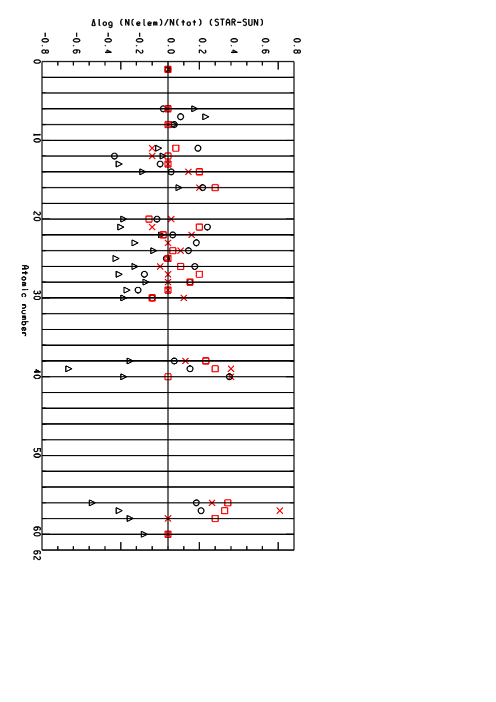
Figure 7 shows that the abundance patterns of the first (red crosses) and second (red boxes) components of AK Sco have the same trend, although they are not identical. In both stars, most of the elements have solar or nearly solar abundances. In addition to Li (not included in Fig. 7), exceptions are found for Si, S, Y, Zr, Ba, and La, which are overabundant. The overabundance in the primary and in the secondary are correspondingly [2.3] and [2.5] for Li, [0.13] and [0.20] for Si, [0.20] and [0.30] for S, [0.4] and [0.3] for Y, [0.28] and [0.38] for Ba, [0.71] and [0.36] for La. Zirconium is overabundant by [0.4] only in the primary, while it was found solar in the secondary. In addition to this large abundance difference for Zr ii, other remarkable differences are those for Sc ii (0.30 dex), Ti ii (0.29 dex), and La ii (0.35 dex). Because we estimate that the errors in the abundance determination are at least of the order of 0.2 dex, we prefer to consider the abundance differences from the two components lower than 0.2 dex as not conclusive.
In Fig. 7 we compare the abundances of the two components of AK Sco with the abundances of the two magnetic Herbig Ae stars HD 104237 (Cowley, Castelli & Hubrig 2013) and PDS2 (Cowley, Hubrig & Przybilla 2014). While the abundance patterns of both components in the studied SB2 system, AK Sco A and AK Sco B, are similar to the abundance pattern of the primary in the SB2 system HD 104237 (open circles), in particular for elements heavier than strontium, they are rather different from the abundance pattern of the single Herbig star PDS2 (triangles), which follows the trend shown by the Boo stars.
In conclusion, although AK Sco B, HD 104237, and PDS2 are magnetic stars, they do not have a similar abundance behaviour: the first two stars display weak Ap/Bp peculiarities, as well as AK Sco A does, although no magnetic field was detected up to now for it. In contrast, PDS2 is characterized by Boo chemical peculiarities. The two different kinds of abundance patterns (Ap/Bp and Boo) do not seem to be dependent on temperature, since PDS2 and AK Sco have the same K.
Acknowledgements
Based on observations made with ESO Telescopes at the La Silla Paranal Observatory under programme IDs 097.C-0277(A) and 099.C-0081(A). We thank the anonymous referee for the useful comments.
References
- Acke & Waelkens (2004) Acke B., Waelkens C., 2004, A&A, 427, 1009
- Aldenius et al. (2009) Aldenius M., Lundberg H., Blackwell-Whitehead R., 2009, A&A, 502, 989
- Alencar et al. (2003) Alencar S. H. P., Melo C. H. F., Dullemond C. P., Andersen J., Batalha C., Vaz L. P. R., Mathieu R. D., 2003, A&A, 409, 1037
- Andersen et al. (1989) Andersen J., Lindgren H., Hazen M. L., Mayor M., 1989, A&A, 219, 142
- Anstee & O’Mara (1995) Anstee S. D., O’Mara B. J., 1995, MNRAS, 276, 859
- Asplund et al. (2009) Asplund M., Grevesse N., Sauval A. J., Scott P., 2009, ARA&A, 47, 481
- Babcock (1958) Babcock H. W., 1958, ApJS, 3, 141
- Barklem, Piskunov & O’Mara (2000) Barklem P. S., Piskunov N., O’Mara B. J., 2000, VizieR Online Data Catalog, J/A+AS/142/467
- Bessell (1979) Bessell M. S., 1979, Dudley Observatory Reports, 14, 279
- Castelli & Kurucz (2004) Castelli F., Kurucz R. L. 2003, in Modelling of Stellar Atmospheres, N. Piskunov, W. W. Weiss, & D. F. Gray, eds., IAU Symp., 210, A20
- Catala (2003) Catala C., 2003, EAS Publications Series, 9, 325
- Cowley et al. (2010) Cowley C. R., Hubrig S., González J. F., Savanov I., 2010, A&A, 523, A65
- Cowley & Hubrig (2012) Cowley C. R., Hubrig S., 2012, Astron. Nachr., 333, 34
- Cowley, Castelli & Hubrig (2013) Cowley C. R., Castelli F., Hubrig S., 2013, MNRAS, 431, 3485
- Cowley, Hubrig & Przybilla (2014) Cowley C. R., Hubrig S., Przybilla N., 2014, MNRAS, 440, 2457
- Duchêne (2015) Duchêne G., 2015, Ap&SS, 355, 291
- Ferrario et al. (2009) Ferrario L., Pringle J. E., Tout C. A., Wickramasinghe D. T., 2009, MNRAS, 400, L71
- Folsom et al. (2012) Folsom C. P., Bagnulo S., Wade G. A., Alecian E., Landstreet J. D., Marsden S. C., Waite I. A., 2012, MNRAS, 422, 2072
- Fuhr, Martin & Wiese (1988) Fuhr J. R., Martin G. A., Wiese W. L., 1988, Journal of Physical and Chemical Reference Data, 17, Suppl. 4
- Garz (1973) Garz T., 1973, A&A, 26, 471
- Gómez de Castro (2009) Gómez de Castro A. I., 2009, ApJ, 698, L108
- Grevesse et al. (2015) Grevesse N., Scott P., Asplund M., Sauval A. J., 2015, A&A, 573, A27
- Herbig & Kameswara Rao (1972) Herbig G. H., Kameswara Rao N., 1972, ApJ, 174, 401
- Hubrig et al. (2014) Hubrig S., et al., 2014, MNRAS, 440, L6
- Hubrig et al. (2015) Hubrig S., Carroll T. A., Schöller M., Ilyin I., 2015, MNRAS, 449, L118
- Järvinen et al. (2018) Järvinen S. P., et al., 2018, ApJ, 858, L18
- Kramida et al. (2018) Kramida A., Ralchenko Yu., Reader J., and NIST ASD Team, 2018, Nist Atomic Spectra Database, [Online] available at https://physics.nist.gov/asd/
- Kurucz (1993) Kurucz R., 1993, Atomic data for opacity calculations. Kurucz CD-ROM No. 1. Cambridge, 1
- Kurucz (1995) Kurucz R. L., 1995, private communication
- Kurucz (2005a) Kurucz R. L., 2005a, Memorie della Societa Astronomica Italiana Supplementi, 8, 14
- Kurucz (2005b) Kurucz R. L., 2005b, Memorie della Societa Astronomica Italiana Supplementi, 8, 189
- Kurucz (2018) Kurucz R. L., 2018, Astron. Soc. of the Pacific Conf. Ser., 515, 47
- Ljung et al. (2006) Ljung G., Nilsson H., Asplund M., Johansson S., 2006, A&A, 456, 1181
- Michaud (1970) Michaud G., 1970, ApJ, 160, 641
- Muzerolle et al. (2004) Muzerolle J., D’Alessio P., Calvet N., Hartmann L., 2004, ApJ, 617, 406
- Pickering, Thorne & Perez (2001) Pickering J. C., Thorne A. P., Perez R., 2001, ApJS, 132, 403
- Pogodin et al. (2012) Pogodin M. A., Hubrig S., Yudin R. V., Schöller M., González J. F., Stelzer B., 2012, Astron. Nachr., 333, 594
- Popper (1980) Popper D. M., 1980, ARA&A, 18, 115
- Raassen & Uylings (1998a) Raassen A. J. J., Uylings P. H. M., 1998a, Journal of Physics B Atomic Molecular Physics, 31, 3137
- Raassen & Uylings (1998b) Raassen A. J. J., Uylings P. H. M., 1998b, VizieR Online Data Catalog, J/A+A/340/300
- Reiter et al. (2018) Reiter M., et al., 2018, ApJ, 852, 5
- Scott et al. (2015a) Scott P., et al., 2015a, A&A, 573, A25
- Scott et al. (2015b) Scott P., Asplund M., Grevesse N., Bergemann M., Sauval A. J., 2015b, A&A, 573, A26
- Stepień & Landstreet (2002) Stepień K., Landstreet J. D., 2002, A&A, 384, 554
Appendix A The lines analyzed in the spectrum of AK Sco
In Table 3, the lines analysed in the spectrum of AK Sco for abundance purposes are listed. Successive columns display wavelength, value, the source for the value, the lower excitation potential in cm-1, the abundance from the primary (Star A), remarks about the given line in the primary, the abundance from the secondary (Star B), and remarks about the given line in the secondary. If the abundance was very uncertain, owing to blends or other causes, no abundance is indicated. For each examined ion the line at the top gives the average abundance for the ion under consideration and the solar abundance. If the element is present in two ionization states and different abundances from the two ions were derived, a line after the entries for the two ions gives the average abundance obtained from all lines of that element. This is the case for Si i, Si ii, Ti i, Ti ii, Cr i, Cr ii, Fe i, Fe ii, Sr i, and Sr ii.
Notes to Table 3:
(a) The index “h” added after the wavelength value indicates that hyperfine structure was considered for that line.
(b) a “K:” at the beginning of the source (Col. 3) indicates that the value was taken from the Kurucz line list available at http://kurucz.harvard.edu/ linelists/gfnew/gfall08oct17.dat and its reference from http://kurucz.harvard.edu/linelists/gfnew/gfall.ref; NIST5: NIST database – http://www.nist.gov/PHYSRefData/ ASD/lines-form.html (Kramida et al. 2018); ALD: Aldenius et al. 2009; FMW: Fuhr, Martin & Wiese 1988; GARZ: Garz 1973; K88: Kurucz 1993; Ljun: Ljung et al. 2006; PTP: Pickering, Thorne & Perez 2001; RU1: Raassen & Uylings 1998a; RU2: Raassen & Uylings 1998b; SUN: astrophysical value derived by fitting the observed solar profiles.
(c) Significance of the notes in Columns 6 and 8: bl A – line blended with other lines in the primary; bl B – line blended with other lines in the secondary; bl AB – line blended with other lines in both primary and secondary; bl unk – line blended with an unidentified line; bl – line blended for other reasons; single – line unblended; almost single – line blended with a very minor component; redsh – line redshifted; core – the observed line core is weaker than the computed one; TSC – the line is computed too strong; red comp – line affected by a red component; cont – line affected by continuum.
| [Å] | Ref.b | Notesc | Notesc | |||||
| Li i | 8.70 | 10.99 (Sun) | 8.50 | 10.99 (Sun) | ||||
| 6707.76 | 0.002 | NIST5 | 0. | 000 | 8.70 | bl Li i | 8.50 | bl Li i |
| 6707.91 | 0.303 | NIST5 | 0. | 000 | 8.70 | bl Li i | 8.50 | bl Li i |
| C i | 3.61 | 3.61 (Sun) | 3.61 | 3.61 (Sun)) | ||||
| 4932.050 | 1.658 | NIST5 | 61981. | 818 | bl AB | bl AB | ||
| 5052.144 | 1.303 | NIST5 | 61981. | 818 | 3.61 | single | bl unk | |
| 5380.325 | 1.616 | NIST5 | 61981. | 818 | bl B | bl A | ||
| 6587.620 | 1.003 | NIST5 | 68856. | 338 | bl AB | 3.61 | single | |
| O i | 3.35 | 3.35 (Sun) | 3.35 | 3.35 (Sun) | ||||
| 6155.961 | 1.363 | NIST5 | 86625. | 757 | 3.35 | weak, bl AB | 3.35 | weak, bl AB |
| 6155.971 | 1.011 | NIST5 | 86625. | 757 | 3.35 | weak, bl AB | weak, bl AB | |
| 6155.989 | 1.120 | NIST5 | 86625. | 757 | 3.35 | weak, bl AB | weak, bl AB | |
| 6156.737 | 1.487 | NIST5 | 86627. | 778 | 3.35 | weak, bl AB | 3.35 | weak, bl AB |
| 6156.755 | 0.898 | NIST5 | 86627. | 778 | 3.35 | weak, bl AB | 3.35 | weak, bl AB |
| 6156.778 | 0.694 | NIST5 | 86627. | 778 | 3.35 | weak, bl AB | 3.35 | weak, bl AB |
| 6158.149 | 1.841 | NIST5 | 86631. | 454 | 3.35 | weak, bl B | 3.35: | weak, bl AB |
| 6158.172 | 0.996 | NIST5 | 86631. | 454 | 3.35 | weak, bl B | 3.35: | weak, bl AB |
| 6158.187 | 0.409 | NIST5 | 86631. | 454 | 3.35 | weak, bl B | 3.35: | weak, bl AB |
| Na i | 5.93 | 5.83 (Sun) | 5.83 (Sun) | |||||
| 4982.813h | 0.962 | NIST5 | 16973. | 366 | bl B | bl A | ||
| 5682.633h | 0.706 | NIST5 | 16956. | 172 | 5.93 | single | 5.73 | bl |
| 5688.193h | 1.406 | NIST5 | 16973. | 368 | bl B | 5.83 | almost single | |
| 5688.295h | 0.452 | NIST5 | 16973. | 368 | bl B | 5.83 | almost single | |
| 5889.950h | 0.108 | NIST5 | 0. | 000 | complex structure | complex structure | ||
| 5895.924h | 0.194 | NIST5 | 0. | 000 | complex structure | complex structure | ||
| 6154.225h | 1.547 | NIST5 | 16956. | 170 | 5.93 | single | bl A | |
| 6160.747h | 1.246 | NIST5 | 16973. | 366 | bl B | bl A | ||
| Mg i | 4.55 | 4.45 (Sun) | 4.45 | 4.45 (Sun) | ||||
| 4057.505 | 0.900 | NIST5 | 35051. | 264 | bl AB | bl AB | ||
| 4167.271 | 0.745 | NIST5 | 35051. | 264 | 4.55 | single | 4.45 | single |
| 4702.991 | 0.440 | NIST5 | 35051. | 264 | bl A, core TSC | bl B | ||
| 5167.321 | 0.870 | NIST5 | 21850. | 405 | bl AB, core TSC, redsh 1.5 km s-1 | bl AB | ||
| 5172.684 | 0.393 | NIST5 | 21870. | 464 | bl AB, core TSC, redsh 1.5 km s-1 | bl AB | ||
| 5183.604 | 0.167 | NIST5 | 21911. | 178 | bl A, core TSC | bl AB | ||
| 5528.405 | 0.498 | NIST5 | 35051. | 264 | 4.55 | bl B, core TSC | 4.45 | single |
| 5711.095 | 1.724 | NIST5 | 35051. | 264 | bl B | 4.46 | single | |
| Mg ii | 4.55 | 4.45 (Sun) | 4.45 | 4.45 (Sun) | ||||
| 4481.126 | 0.749 | NIST5 | 71490. | 190 | 4.55 | bl B | 4.45 | bl A |
| 4481.150 | 0.553 | NIST5 | 71490. | 190 | 4.55 | bl B | 4.45 | |
| 4481.325 | 0.594 | NIST5 | 71491. | 063 | 4.55 | bl B | 4.45 | |
| Al i | 5.61 | 5.61 (Sun) | 5.61 | 5.61 (Sun) | ||||
| 3944.006h | 0.638 | NIST5 | 0. | 000 | 5.61 | bl B, redsh 3 km s-1 | 5.61 | bl AB |
| 3961.520h | 0.336 | NIST5 | 112. | 061 | 5.61 | bl B | 5.61 | bl A |
| 6696.018h | 1.569 | NIST5 | 25347. | 756 | bl AB | bl AB | ||
| 6698.667h | 1.870 | NIST5 | 25347. | 756 | single, bad cont ? | single, bad cont ? | ||
| [Å] | Ref.b | Notesc | Notesc | |||||
| Si i | 4.53 (Sun) | 4.53 (Sun) | ||||||
| 5645.613 | 2.140 | GARZ | 39760. | 285 | bl B | 4.33 | almost single | |
| 5665.555 | 2.040 | NIST5 | 39683. | 163 | bl B | bl A | ||
| 5690.425 | 1.870 | NIST5 | 39760. | 285 | 4.33 | single | 4.23 | single |
| 5708.400 | 1.470 | NIST5 | 39955. | 053 | 4.28 | almost single | bl AB | |
| 5772.146 | 1.750 | NIST5 | 40991. | 884 | 4.28 | single | 4.23 | almost single |
| 5948.541 | 1.231 | NIST5 | 40991. | 884 | 4.43 | single | bl with telluric | |
| 6091.919 | 1.250 | SUN | 47351. | 554 | bl AB | bl A | ||
| 6125.021 | 1.565 | SUN | 45276. | 188 | bl AB | bl A | ||
| 6142.483 | 1.480 | SUN | 45321. | 848 | 4.43 | single | 4.33 | single |
| 6145.016 | 1.411 | SUN | 45293. | 629 | 4.43 | single | 4.33 | single |
| 6155.134 | 0.855 | SUN | 45321. | 848 | 4.43 | single | almost single, bad cont | |
| 6237.319 | 1.070 | SUN | 45276. | 188 | 4.48 | single, redsh | 4.43 | single |
| 6243.815 | 1.244 | K:K07 | 45293. | 629 | 4.48 | single | bl A | |
| 6244.466 | 1.291 | SUN | 45293. | 629 | 4.38 | single | bl A | |
| 6414.980 | 1.036 | K:K07 | 47351. | 554 | 4.48 | single | bl A | |
| 6721.848 | 1.140 | SUN | 47284. | 061 | 4.33 | single | 4.33 | single |
| Si ii | 4.40 | 4.53 (Sun) | 4.40 | 4.53 (Sun) | ||||
| 5055.984 | 0.523 | NIST5 | 81251. | 320 | bl AB | bl AB, telluric | ||
| 6347.109 | 0.149 | NIST5 | 65500. | 470 | 4.40 | single | 4.40 | single |
| 6371.359 | 0.082 | NIST5 | 65500. | 470 | bl B | 4.40 | single | |
| Si(tot) | 4.53 (Sun) | 4.53 (Sun) | ||||||
| S i | 4.92 (Sun) | 4.92 (Sun) | ||||||
| 6046.038 | 0.959 | NIST5 | 63457. | 142 | bl B | 4.52 | single | |
| 6052.594 | 1.258 | NIST5 | 63475. | 051 | 4.82 | single | bl B | |
| 6743.552 | 1.065 | NIST5 | 63446. | 065 | bl AB | bl A | ||
| 6748.578 | 0.843 | NIST5 | 63457. | 142 | bl unk | bl unk | ||
| 6748.792 | 0.638 | NIST5 | 63457. | 142 | bl unk | bl A, unk | ||
| 6756.961 | 0.937 | NIST5 | 63477. | 051 | 4.62 | bl S i | 4.72 | bl S i |
| 6757.153 | 0.351 | NIST5 | 63475. | 051 | 4.62 | bl S i | 4.72 | bl S i |
| Ca i | 5.72 (Sun) | 5.72 (Sun) | ||||||
| 4226.728 | 0.244 | NIST5 | 0. | 000 | bl AB | bl AB | ||
| 4283.011 | 0.224 | NIST5 | 15210. | 063 | bl AB | bl AB | ||
| 4318.652 | 0.208 | NIST5 | 15315. | 943 | bl A | 5.65 | single | |
| 4425.437 | 0.358 | NIST5 | 15157. | 901 | 5.72 | almost single | 5.72 | almost single |
| 4434.957 | 0.010 | NIST5 | 15210. | 063 | bl AB | bl B | ||
| 4435.679 | 0.519 | NIST5 | 15210. | 063 | bl unk ? | bl A | ||
| 4578.551 | 0.558 | NIST5 | 20335. | 360 | 5.72 | single | bl unk ? | |
| 4585.865 | 0.187 | NIST5 | 20371. | 000 | bl B | bl A | ||
| 4685.268 | 0.88 | NIST5 | 44989. | 830 | 5.57 | single | bl A | |
| 5512.980 | 0.300 | NIST5 | 23652. | 304 | 5.82 | almost single | bl A | |
| 5581.965 | 0.517 | K:K07 | 20349. | 260 | 5.57 | almost single | 5.62 | almost single |
| 5590.114 | 0.547 | K:K07 | 20335. | 360 | bl B | 5.62 | almost single | |
| 5598.480 | 0.091 | K:K07 | 20335. | 360 | bl A | bl B | ||
| 5867.562 | 1.600 | SUN | 23652. | 304 | bl B | 5.62 | single | |
| 6102.723 | 0.790 | NIST5 | 15157. | 901 | 5.57 | single | 5.62 | single |
| 6122.217 | 0.315 | NIST5 | 15210. | 063 | 5.65 | single | 5.55 | single |
| 6162.173 | 0.170 | ALD | 15315. | 943 | 5.65 | almost single | bl AB | |
| 6169.042 | 0.54 | NIST5 | 20349. | 268 | 5.77 | almost single | bl A | |
| 6169.563 | 0.27 | NIST5 | 20371. | 000 | 5.72 | almost single | bl A | |
| 6439.075 | 0.47 | NIST5 | 20371. | 000 | 5.70 | single | 5.60 | single |
| 6449.808 | 0.55 | NIST5 | 20335. | 360 | 5.70 | almost single | 5.70 | almost single |
| 6471.662 | 0.59 | NIST5 | 20371. | 000 | 5.70 | single | 5.70 | single, bl telluric |
| 6499.650 | 0.59 | NIST5 | 20371. | 000 | 5.95 | single | 5.80 | single |
| 6717.681 | 0.61 | NIST5 | 21849. | 634 | 5.70 | almost single | 5.45 | almost single, |
| redsh 1.5 km s-1, red comp ? | ||||||||
| [Å] | Ref.b | Notesc | Notesc | |||||
| Ca ii | 5.72 (Sun) | 5.72(Sun) | ||||||
| 3933.664 | 0.111 | K:K10 | 0. | 000 | core not fitted | not fitted | ||
| 3968.469 | 0.194 | K:K10 | 0. | 000 | core not fitted | not fitted | ||
| Sc ii | 8.98 | 8.88 (Sun) | 8.68 | 8.88 (Sun) | ||||
| 4246.822h | 0.242 | NIST5 | 2540. | 950 | bl, red comp ? | bl, red comp ? | ||
| 4314.083h | 0.096 | NIST5 | 4987. | 790 | bl AB | bl AB | ||
| 4320.732h | 0.252 | NIST5 | 4883. | 570 | bl A | bl AB | ||
| 4400.389h | 0.536 | NIST5 | 4883. | 570 | 8.98 | almost single | bl A | |
| 4670.407h | 0.576 | NIST5 | 10944. | 560 | bl AB | bl AB | ||
| 5031.021 | 0.399 | NIST5 | 10944. | 560 | bl AB | 8.68 | almost single | |
| 5239.813 | 0.765 | NIST5 | 11736. | 360 | 8.98 | almost single | 8.68 | almost single |
| 5526.790h | 0.025 | NIST5 | 14261. | 250 | bl B, red comp ? | bl A | ||
| 6604.601h | 1.309 | NIST5 | 10944. | 560 | 8.98 | single | bl B | |
| Ti i | 7.11 (Sun) | 7.11 | 7.11 (Sun) | |||||
| 4286.004 | 0.350 | K:LGWS | 6661. | 006 | 7.11 | single | bl | |
| 4512.734 | 0.424 | K:BMPS | 6742. | 756 | 7.21 | almost single | spike | |
| 4981.731 | 0.560 | K:BMPS | 6842. | 962 | bl B | bl A | ||
| 4999.503 | 0.306 | K:BMPS | 6661. | 004 | bl B | bl A | ||
| 5035.903 | 0.220 | K:LGWS | 11776. | 812 | bl A | bl B | ||
| 5039.957h | 1.074 | K:BMP | 170. | 13 | bl B | no fit, bl A | ||
| 5866.451h | 0.784 | K:BMPS | 8602. | 344 | 7.11 | single | bl A | |
| Ti ii | 7.11 (Sun) | 7.11 (Sun) | ||||||
| 4025.129 | 2.110 | K:WLSC | 4897. | 650 | bl AB | bl B | ||
| 4287.873h | 1.790 | PTP | 8710. | 440 | bl AB | bl AB | ||
| 4290.215h | 0.870 | K:WLSC | 9395. | 710 | bl AB | bl AB | ||
| 4300.042h | 0.460 | K:WLSC | 9518. | 060 | bl AB | bl AB | ||
| 4312.860h | 1.120 | K:WLSC | 9518. | 152 | 6.81 | single | bl A | |
| 4398.289 | 2.650 | K:PTP | 9872. | 899 | bl A | bl AB | ||
| 4399.765h | 1.200 | K:WLSC | 9975. | 999 | bl A | bl A | ||
| 4411.073h | 0.650 | K:WLSC | 24961. | 030 | bl A | bl B | ||
| 4411.930 | 2.620 | K:WLSC | 9872. | 73 | bl A | bl B | ||
| 4417.713h | 1.167 | K:K16 | 9395. | 802 | bl B | bl A | ||
| 4421.938 | 1.640 | K:WLSC | 16625. | 11 | bl A | bl AB | ||
| 4441.728 | 2.333 | K:K16 | 9518. | 06 | 6.81 | almost single | bl A | |
| 4443.801h | 0.710 | K:WLSC | 8710. | 44 | red comp ?, not in syn1 | bl unk ? | ||
| 4450.482h | 1.520 | K:WLSC | 8744. | 25 | bl AB | bl AB | ||
| 4468.492h | 0.600 | K:BHNG | 9118. | 26 | 6.81 | single | bl A | |
| 4488.325h | 0.500 | K:WLSC | 25192. | 79 | bl A | bl AB | ||
| 4501.270h | 0.770 | K:WLSC | 8997. | 71 | bl AB | bl AB | ||
| 4518.332 | 2.560 | K:WLSC | 8710. | 440 | bl A | bl AB | ||
| 4533.960h | 0.577 | K:K16 | 9975. | 92 | bl AB | bl AB | ||
| 4563.758h | 0.795 | K:K16 | 10024. | 73 | bl AB | bl AB | ||
| 4571.971h | 0.310 | K:WLSC | 12676. | 97 | bl AB, red comp ? | bl B, red comp ? | ||
| 4708.663 | 2.350 | K:WLSC | 9975. | 92 | bl B | bl A | ||
| 4779.979 | 1.248 | K:K16 | 16515. | 86 | 6.81 | single | 7.01 | single |
| 4798.531 | 2.660 | K:WLSC | 8710. | 44 | bl A | bl AB | ||
| 5010.209 | 1.350 | K:WLSC | 25192. | 79 | bl A | bl AB | ||
| 5211.530 | 1.410 | K:WLSC | 20891. | 787 | bl B | 7.21 | almost single | |
| 5381.022 | 1.970 | K:WLSC | 12628. | 73 | bl B | bl A | ||
| 5418.768 | 2.130 | K:WLSC | 12758. | 11 | 7.01 | single | bl A | |
| 5490.693 | 2.663 | K:K16 | 12628. | 834 | bl A | bl A | ||
| 6491.566 | 1.942 | K:K16 | 16625. | 110 | 7.01: | bl telluric | 7.21 | single |
| Ti(tot) | 7.11 (Sun) | 7.11 (Sun) | ||||||
| [Å] | Ref.b | Notesc | Notesc | |||||
| V i | 8.15 | 8.15(Sun) | — | 8.15 (Sun) | ||||
| 4379.230h | 0.580 | NIST5 | 2424. | 780 | 8.15 | single | bl A | |
| 6090.208h | 0.067 | NIST5 | 8715. | 760 | 8.15 | single | bl A | |
| 6119.527h | 0.350 | NIST5 | 8578. | 530 | bl B | bl AB, weak | ||
| V ii | — | — | 8.15 (Sun) | |||||
| 4002.928 | 1.440 | K:WLDS | 11514. | 760 | bl AB | bl AB | ||
| 4023.377 | 0.610 | K:WLDS | 14556. | 090 | bl B | bl A | ||
| 4183.428 | 1.060 | K:WLDS | 16533. | 00 | bl AB | bl A | ||
| 4312.348 | 1.495 | K:BGFM | 13490. | 883 | bl AB | bl B | ||
| Cr i | 6.42 (Sun) | 6.42 | 6.42 (Sun) | |||||
| 4254.336 | 0.108 | K:BMP | 0. | 000 | bl AB | bl AB | ||
| 4274.797 | 0.231 | K:BMP | 0. | 000 | bl AB | bl AB | ||
| 4616.124 | 1.204 | K:BMP | 7927. | 441 | 6.42 | single | bl A | |
| 4626.173 | 1.340 | K:BMP | 7810. | 820 | bl B | bl A | ||
| 4652.157 | 1.035 | K:SLS | 8095. | 187 | bl B | 6.42 | almost single | |
| 4718.420 | 0.240 | K:SLS | 25771. | 420 | 6.42 | almost single, redsh ? | 6.42 | almost single, redsh ? |
| 5204.511 | 0.198 | K:BMP | 7593. | 160 | bl A | bl AB | ||
| 5208.425 | 0.172 | K:BMP | 7593. | 148 | bl A, flat core | bl B | ||
| 5409.784 | 0.715 | K:BMP | 8307. | 575 | 6.22 | almost single | bl AB | |
| 5787.919 | 0.083 | K:BBMP | 26796. | 266 | 6.57 | single | 6.42 | single |
| 5790.957 | 0.250 | K:K16 | 25787. | 964 | bl A, flat core | bl B | ||
| Cr ii | 6.42 (Sun) | 6.42 (Sun) | ||||||
| 4242.366 | 1.352 | K:K16 | 31219. | 350 | bl AB | bl AB | ||
| 4252.625 | 2.053 | K:K16 | 31117. | 390 | bl B | bl A | ||
| 4558.644 | 0.444 | K:K16 | 32854. | 31 | 6.42 | bl Cr ii | 6.32 | almost single |
| 4558.788 | 2.741 | RU1 | 32854. | 94 | 6.42 | bl Cr ii | 6.32 | |
| 4588.198 | 0.826 | K:NLLN | 32836. | 68 | bl B | 6.32 | single | |
| 4616.624 | 1.575 | RU1 | 32844. | 76 | bl AB | bl B | ||
| 4618.807 | 0.996 | K:NLLN | 32854. | 95 | bl A | bl AB | ||
| 4634.070 | 0.980 | K:NLLN | 32844. | 76 | bl B | bl A | ||
| 4824.131 | 1.085 | RU1 | 31219. | 332 | bl A | bl AB | ||
| 5237.322 | 1.160 | NIST5 | 32854. | 31 | bl AB | 6.42 | almost single | |
| 5502.085 | 2.048 | K:K16 | 33618. | 91 | 6.02 | single | bl A | |
| Cr(tot) | 6.42 (Sun) | 5.42 (Sun) | ||||||
| Mn i | 6.62 | 6.62 (Sun) | 6.62 | 6.62 (Sun) | ||||
| 4033.062h | 0.647 | K:DLSS | 0. | 000 | bl AB | bl B | ||
| 4034.483h | 0.843 | K:DLSS | 0. | 000 | 6.62 | single | bl A | |
| 4041.355h | 0.281 | K:DLSS | 17052. | 29 | bl A | bl B | ||
| 4754.042h | 0.080 | K:DLSS | 23719. | 52 | 6.62 | almost single | 6.62 | almost single |
| 4783.427h | 0.044 | K:DLSS | 18531. | 5 | 6.62 | almost single | 6.62 | single |
| 4823.524h | 0.136 | K:DLSS | 18705. | 2 | bl A | bl B | ||
| 5377.596h | 0.166 | K:K07 | 31001. | 153 | bl B | bl A | ||
| 5537.765h | 2.017 | K88 | 17637. | 156 | bl AB | bl AB | ||
| 6013.510h | 0.354 | K:DLSS | 24779. | 331 | red comp ?, | red comp ?, | ||
| only | only | |||||||
| [Å] | Ref.b | Notesc | Notesc | |||||
|---|---|---|---|---|---|---|---|---|
| Fe i | 4.57 (Sun) | 4.57 (Sun) | ||||||
| 4071.738 | 0.022 | K:FW | 12968. | 554 | bl AB | bl AB | ||
| 4383.544 | 0.200 | K:FW | 11976. | 239 | bl A | bl AB | ||
| 4736.773 | 0.67 | K:DRLP | 25899. | 899 | bl B | 4.57 | single | |
| 4890.755 | 0.38 | K:RDLB | 23192. | 500 | bl A | bl B | ||
| 4891.492 | 0.112 | K:FW | 22996. | 674 | 4.67 | single | bl A | |
| 4903.310 | 0.89 | K:RDLB | 23244. | 838 | bl A | bl AB | ||
| 4907.732 | 1.70 | K:DRLP | 27666. | 348 | bl A | bl AB | ||
| 4909.383 | 1.325 | K:K17 | 31686. | 351 | bl B | bl A | ||
| 4917.230 | 1.66 | K:FW | 33801. | 572 | 4.57 | single | bl A | |
| 4918.954 | 0.602 | K:K17 | 33507. | 123 | 4.57 | bl Fe i | bl AB | |
| 4918.994 | 0.342 | K:FW | 23110. | 939 | 4.57 | bl Fe i | 4.57 | bl AB |
| 4920.502 | 0.07 | K:RDLB | 22845. | 869 | bl AB, core | very bl AB | ||
| 4946.387 | 1.11 | K:RDLB | 27166. | 820 | bl AB | bl A | ||
| 4950.105 | 1.50 | K:DRLP | 27559. | 583 | single, bad cont ? | 4.37 | single | |
| 4957.596 | 0.233 | K:FW | 22650. | 416 | bl A, core | bl AB | ||
| 4962.571 | 1.182 | K:FW | 33695. | 397 | bl B | 4.27 | single | |
| 4969.917 | 0.588 | K:K17 | 34017. | 103 | bl B | bl A | ||
| 4970.496 | 1.74 | K:FW | 29320. | 025 | bl A | bl B | ||
| 4991.268 | 0.368 | K:K17 | 33801. | 572 | bl AB, core | bl B | ||
| 4994.129 | 3.080 | K:FW | 7376. | 764 | bl B | bl B | ||
| 5007.274 | 0.198 | K:K17 | 33095. | 941 | bl AB, core | bl AB | ||
| 5028.126 | 1.02 | K:RDLB | 28819. | 954 | bl B | bl A | ||
| 5068.766 | 1.042 | K:FW | 23711. | 456 | bl AB | bl B | ||
| 5098.698 | 2.03 | K:FW | 17550. | 181 | bl AB, red comp ? | bl AB | ||
| 5107.447 | 3.087 | K:FW | 7985. | 785 | bl A | bl B | ||
| 5107.641 | 2.418 | K:FW | 12560. | 934 | 4.57 | bl A | 4.27 | bl B |
| 5110.413 | 3.760 | K:FW | 0. | 000 | bl A, core | bl B | ||
| 5126.192 | 1.06 | K:FW | 34328. | 752 | bl B, unk, redsh ? | bl A, unk ? | ||
| 5137.381 | 0.43 | K:FW | 33695. | 397 | bl AB, redsh | bl B | ||
| 5142.494 | 0.739 | K:K17 | 34692. | 148 | bl AB, redsh | bl AB, core | ||
| 5142.540 | 0.295 | K:K17 | 34328. | 752 | 4.57 | bl AB, redsh | 4.27 | bl AB, core |
| 5196.059 | 0.477 | K:K17 | 34328. | 752 | bl AB, redsh ? | bl AB | ||
| 5216.274 | 2.150 | K:FW | 12968. | 554 | bl AB, red comp ? | bl AB | ||
| 5217.389 | 1.07 | K:DRLP | 25899. | 989 | bl AB, redsh ? | 4.57 | single | |
| 5232.940 | 0.057 | K:FW | 23711. | 456 | 4.67 | almost single | bl A | |
| 5364.870 | 0.228 | K:FW | 35856. | 402 | 4.67 | single | 4.57 | single |
| 5367.465 | 0.443 | K:FW | 35611. | 625 | 4.97 | almost single, core | 4.87 | almost single, core |
| 5369.961 | 0.536 | K:FW | 35257. | 324 | 4.77 | almost single | bl A | |
| 5371.489 | 1.645 | K:FW | 7728. | 060 | bl AB | bl AB | ||
| 5373.708 | 0.71 | K:RDLB | 36079. | 372 | bl AB | bl B | ||
| 5383.368 | 0.645 | K:FW | 34782. | 421 | bl B | 4.57 | almost single | |
| 5389.478 | 0.430 | K:K17 | 35611. | 625 | 4.67 | almost single | 4.47 | almost single |
| 5400.501 | 0.151 | K:K17 | 35257. | 324 | bl AB | bl AB | ||
| 5405.774 | 1.844 | K:FW | 7985. | 785 | bl AB | bl A | ||
| 5410.909 | 0.398 | K:FW | 36079. | 372 | bl AB, redsh, red comp ? | 4.47 | almost single | |
| 5415.198 | 0.642 | K:FW | 35279. | 308 | bl AB | 4.67 | almost single | |
| 5424.067 | 0.780 | K:K17 | 34843. | 957 | bl A, core | bl AB, core | ||
| 5429.696 | 1.879 | K:FW | 7728. | 060 | bl A | bl AB | ||
| 5445.042 | 0.209 | K:K17 | 35379. | 208 | 4.82 | single, core | bl AB | |
| 5446.916 | 1.914 | K:FW | 7985. | 785 | bl AB | bl AB | ||
| 5466.395 | 0.630 | FMW | 35257. | 324 | bl A | bl A | ||
| 5487.745 | 0.316 | K:K17 | 34843. | 957 | 4.67 | single, core | bl AB | |
| 5497.516 | 2.849 | K:FW | 8154. | 714 | bl A | bl B, core | ||
| 5506.779 | 2.797 | K:FW | 7985. | 785 | bl A | bl B | ||
| 5522.446 | 1.52 | K:FW | 33946. | 933 | bl B | bl A | ||
| 5560.212 | 1.16 | K:FW | 35767. | 564 | 4.47 | single, core | bl A | |
| 5572.842 | 0.28 | K:DRLP | 27394. | 691 | bl A, core | bl AB | ||
| 5914.111 | 0.362 | K:K17 | 37162. | 764 | bl A, core | bl B | ||
| 5914.201 | 0.111 | K:K17 | 37162. | 764 | 4.47 | bl A, core | 4.67 | bl B |
| 6191.557 | 1.416 | K:FW | 19621. | 006 | bl A | bl B | ||
| 6393.600 | 1.58 | K:FW | 19621. | 006 | 4.37 | single, redsh 1 km s-1 ?, comp ? | 4.27 | single |
| [Å] | Ref.b | Notesc | Notesc | |||||
| Fe ii | 4.42 | 4.37 (Sun) | 4.57 (Sun) | |||||
| 4178.854 | 2.535 | RU2 | 20830. | 582 | bl B, unk | bl A | ||
| 4413.591 | 3.985 | SUN | 21581. | 638 | 4.42 | single | very bl | |
| 4416.819 | 2.601 | RU2 | 22409. | 852 | bl B | bl A | ||
| 4515.533 | 2.540 | RU2 | 22409. | 852 | bl AB, redsh | bl AB | ||
| 4620.513 | 3.188 | K:FW | 22810. | 357 | bl B | bl A, redsh ? | ||
| 4635.317 | 1.474 | K:FW | 48039. | 090 | bl B | bl A | ||
| 4923.921 | 1.206 | K:FW | 23317. | 635 | bl AB | bl AB | ||
| 5100.655 | 4.222 | K:FW | 22637. | 195 | bl B | 4.32 | bl Fe ii | |
| 5120.344 | 4.275 | K:K13 | 22810. | 357 | bl AB | bl AB | ||
| 5132.661 | 4.008 | K:FW | 22637. | 205 | bl B | bl A | ||
| 5197.568 | 2.229 | K:FW | 26055. | 412 | bl A, red wing, unk ? | bl A | ||
| 5362.869 | 2.616 | RU2 | 25805. | 327 | bl AB | bl AB | ||
| 5425.249 | 3.352 | K:FW | 25805. | 327 | bl B | 4.47 | single | |
| 5534.838 | 2.86 | K:FW | 26170. | 18 | 4.42 | single | 4.47 | single |
| 6084.102 | 3.854 | K:FW | 25805. | 327 | bl B | bl unk ? | ||
| 6147.734 | 2.731 | K:FW | 31364. | 455 | bl A, Fe i | bl AB | ||
| 6149.246 | 2.732 | K:FW | 31368. | 453 | bl B | 4.47 | single | |
| 6383.730 | 2.275 | K:FW | 60445. | 279 | bl A, Fe i | bl AB | ||
| 6456.380 | 2.086 | K:FW | 31483. | 198 | bl B | 4.47 | single | |
| Fe(tot) | 4.57 (Sun) | 4.57 (Sun) | ||||||
| Co i | — | 7.11 (Sun) | 6.91 | 7.11 (Sun) | ||||
| 3995.302h | 0.220 | NIST5 | 7442. | 410 | bl AB | 6.91 | single | |
| 4118.767h | 1.093 | K:K08 | 8460. | 783 | bl AB | bl A | ||
| 4121.311h | 0.320 | NIST5 | 7442. | 410 | bl B | bl A | ||
| Ni i | 5.84 (Sun) | 5.84 (Sun) | ||||||
| 4295.882h | 0.480 | NIST5 | 30979. | 749 | bl AB | bl AB | ||
| 4648.652 | 0.150 | NIST5 | 27580. | 391 | bl B | bl A | ||
| 4701.530 | 0.390 | NIST5 | 32973. | 376 | bl AB | bl AB | ||
| 4756.515 | 0.270 | NIST5 | 28068. | 065 | 5.84 | almost single | bl A | |
| 4806.987 | 0.640 | NIST5 | 29668. | 893 | 5.84 | single | bl A | |
| 4829.023h | 0.330 | NIST5 | 28569. | 203 | 5.84 | almost single | 5.84 | almost single |
| 4831.176 | 0.410 | NIST5 | 29084. | 450 | 5.94 | single | bl A | |
| 4904.412h | 0.170 | NIST5 | 28569. | 203 | bl B | 5.84 | single | |
| 5035.362h | 0.290 | NIST5 | 29320. | 762 | 5.94 | single | 5.84 | single |
| 5035.967h | 0.234 | K88 | 29480. | 989 | bl A | bl B | ||
| 5081.110 | 0.300 | NIST5 | 31031. | 020 | bl B | bl A | ||
| 5082.344h | 0.540 | NIST5 | 29500. | 674 | bl B | bl A | ||
| 5085.480h | 1.480 | NIST5 | 29500. | 674 | bl B | 5.84 | single | |
| 5099.920 | 0.100 | NIST5 | 29668. | 893 | bl B | 5.74 | single | |
| 5102.960h | 2.620 | NIST5 | 13521. | 347 | 5.94 | single | bl A | |
| 5115.392 | 0.110 | NIST5 | 30922. | 734 | bl B | bl A | ||
| 5146.482h | 0.060 | K:K08 | 29888. | 477 | bl A | bl B | ||
| 5155.764 | 0.090 | NIST5 | 31441. | 635 | bl B | 5.44 | single | |
| 5578.726 | 2.640 | NIST5 | 13521. | 347 | 5.74 | single | 5.44 | single, spike, cont |
| 6643.543h | 2.300 | NIST5 | 13521. | 347 | 5.74 | single | 5.59 | single |
| 6772.315 | 0.990 | NIST5 | 29500. | 674 | 5.74 | single | bl A | |
| Cu i | 7.86 | 7.86 (Sun) | 7.86 | 7.86 (Sun) | ||||
| 5105.548 | 1.500 | NIST5 | 11202. | 565 | 7.86: | bl B | 7.86 | single |
| 5153.238 | 0.116 | K:K12 | 30535. | 302 | bl B | bl A | ||
| 5218.202 | 0.264 | NIST5 | 30783. | 686 | bl A | bl A | ||
| [Å] | Ref.b | Notesc | Notesc | |||||
| Zn i | 7.38: | 7.48 (Sun) | 7.58 | 7.48 (Sun) | ||||
| 4680.136 | 0.810 | K:K12 | 32311. | 319 | bl AB | bl AB | ||
| 4722.157 | 0.338 | K:K12 | 32501. | 330 | bl B | bl A | ||
| 4810.532 | 0.125 | K:K12 | 32890. | 327 | 8.08? | single, bad cont ? | 8.08 ? | single, bad cont ? |
| 6362.346 | 0.160 | NIST5 | 46771. | 199 | 7.38: | bl B | 7.58 | single |
| Sr i | — | 9.21 (Sun) | 9.0 | 9.21 (Sun) | ||||
| 4607.333 | 0.283 | NIST5 | 0. | 000 | bl B | 9.00 | single | |
| Sr ii | 9.10 | 9.21 (Sun) | 8.90 | 9.21 (Sun) | ||||
| 4077.709 | 0.148 | NIST5 | 0. | 000 | bl AB | bl AB | ||
| 4215.519 | 0.173 | NIST5 | 0. | 000 | 9.1 | bl A | 8.9 | bl AB |
| 4305.443 | 0.11 | NIST5 | 24516. | 65 | bl AB | bl B | ||
| Sr(tot) | 9.1 | 9.21 (Sun) | 9.21 (Sun) | |||||
| Y ii | 9.40 | 9.83 (Sun) | 9.50 | 9.83 (Sun) | ||||
| 4177.530h | 0.163 | NIST5 | 3296. | 180 | bl AB | bl B | ||
| 4309.622 | 0.747 | NIST5 | 1449. | 752 | bl A | bl B | ||
| 4374.933h | 0.155 | NIST5 | 3296. | 184 | bl AB | bl AB | ||
| 4398.010 | 0.999 | NIST5 | 1045. | 083 | bl A | bl A | ||
| 4854.861h | 0.38 | NIST5 | 8003. | 126 | bl B | bl B | ||
| 4883.682h | 0.07 | NIST5 | 8743. | 316 | 9.40 | single | bl A, cont ? | |
| 4900.119h | 0.09 | NIST5 | 8328. | 041 | cont ?, bl A | cont ?, bl B | ||
| 5087.419h | 0.17 | NIST5 | 8743. | 316 | 9.40 | single | 9.50 | bl A |
| 5119.112h | 1.36 | NIST5 | 8003. | 121 | bl A | bl AB | ||
| 5205.723h | 0.35 | NIST5 | 8328. | 039 | bl AB | bl B | ||
| 5509.895h | 1.015 | NIST5 | 8003. | 126 | bl A | bl B | ||
| Zr ii | 9.04 | 9.45 (Sun) | 9.45 | 9.45 (Sun) | ||||
| 4149.198 | 0.040 | Ljun | 6467. | 610 | bl A | bl AB | ||
| 4156.232 | 0.780 | Ljun | 5724. | 380 | bl unk | bl unk | ||
| 4208.980 | 0.510 | Ljun | 5752. | 920 | 9.04 | single | 9.45 | single |
| 4258.041 | 1.200 | Ljun | 4505. | 500 | bl A | bl AB | ||
| 4442.992 | 0.420 | Ljun | 11984. | 460 | bl AB | bl AB | ||
| 4496.962 | 0.890 | Ljun | 5752. | 92 | bl A | bl AB | ||
| 5112.270 | 0.850 | Ljun | 13428. | 500 | 9.04 | single | bl A | |
| Ba i | 9.79 (Sun) | 9.79 (Sun) | ||||||
| 5535.481 | 0.215 | NIST5 | 0. | 000 | bl A | bl AB | ||
| Ba ii | 9.51 | 9.79 (Sun) | 9.41 | 9.79 (Sun) | ||||
| 4130.649 | 0.524 | NIST5 | 21952. | 36 | bl A | bl A | ||
| 4554.033h | 0.140 | NIST5 | 0. | 000 | 9.51 | almost single | 9.41 | almost single |
| 4934.077h | 0.157 | NIST5 | 0. | 000 | bl AB | bl A | ||
| 5853.675 | 0.908 | NIST5 | 4873. | 852 | bl B | bl A | ||
| 6141.710 | 0.032 | NIST5 | 5674. | 807 | bl A | bl B | ||
| 6496.898h | 0.407 | NIST5 | 4873. | 852 | bl telluric | bl telluric | ||
| [Å] | Ref.b | Notesc | Notesc | |||||
| La ii | 10.93 (Sun) | 10.57 | 10.93 (Sun) | |||||
| 3988.515h | 0.210 | NIST5 | 3250. | 35 | bl A | bl A | ||
| 3995.745 | 0.064 | NIST5 | 1394. | 46 | cont | bl AB | ||
| 4042.901 | 0.270 | L:CB’ | 7473. | 32 | 10.37 | single | bl A | |
| 4086.709h | 0.070 | NIST5 | 0. | 000 | bl B | 10.57 | single | |
| 4123.218h | 0.130 | NIST5 | 2591. | 60 | bl AB | bl B | ||
| 4333.75 | 0.059 | NIST5 | 1394. | 46 | 10.07 | single | bl A | |
| Ce ii | 10.46 | 10.46 (Sun) | — | 10.46 (Sun) | ||||
| 4186.596 | 0.813 | K:MC | 6967. | 547 | bl A | bl B | ||
| 4562.358 | 0.210 | NIST5 | 3854. | 012 | bl B | bl A | ||
| 4628.161 | 0.140 | NIST5 | 4165. | 55 | 10.46 | single | bl A | |
| Nd ii | 10.62 ? | 10.62 (Sun) | 10.62 ? | 10.62 (Sun) | ||||
| 4061.080 | 0.550 | NIST5 | 3801. | 93 | 10.62 | bl A | 10.62 | bl B |
| 4109.071 | 0.163 | NIST5 | 513. | 330 | 9.98 | bl AB | 9.98 | bl AB |
| 4303.571 | 0.084 | NIST5 | 0. | 000 | 10.62 | bl B | 10.62 | bl A |
| 4706.543 | 0.710 | NIST5 | 0. | 000 | 9.92 | bl B | 9.92 | single |
| 5076.580 | 0.250 | K:MC’ | 5985. | 59 | 10.62 | bl A | 10.62 | bl B |