PDE methods in random matrix theoryThanks: Supported in part by a Simons Foundation Collaboration Grant for Mathematicians
Abstract.
This article begins with a brief review of random matrix theory, followed by a discussion of how the large- limit of random matrix models can be realized using operator algebras. I then explain the notion of “Brown measure,” which play the role of the eigenvalue distribution for operators in an operator algebra.
I then show how methods of partial differential equations can be used to compute Brown measures. I consider in detail the case of the circular law and then discuss more briefly the case of the free multiplicative Brownian motion, which was worked out recently by the author with Driver and Kemp.
1. Random matrices
Random matrix theory consists of choosing an matrix at random and looking at natural properties of that matrix, notably its eigenvalues. Typically, interesting results are obtained only for large random matrices, that is, in the limit as tends to infinity. The subject began with the work of Wigner [43], who was studying energy levels in large atomic nuclei. The subject took on new life with the discovery that the eigenvalues of certain types of large random matrices resemble the energy levels of quantum chaotic systems—that is, quantum mechanical systems for which the underlying classical system is chaotic. (See, for example, [20] or [39].) There is also a fascinating conjectural agreement, due to Montgomery [35], between the statistical behavior of zeros of the Riemann zeta function and the eigenvalues of random matrices. See also [30] or [6].
We will review briefly some standard results in the subject, which may be found in textbooks such as those by Tao [40] or Mehta [33].
1.1. The Gaussian unitary ensemble
The first example of a random matrix is the Gaussian unitary ensemble (GUE) introduced by Wigner [43]. Let denote the real vector space of Hermitian matrices, that is, those with where is the conjugate transpose of We then consider a Gaussian measure on given by
| (1) |
where denotes the Lebesgue measure on and where is a normalizing constant. If is a random matrix having this measure as its distribution, then the diagonal entries are normally distributed real random variables with mean zero and variance The off-diagonal entries are normally distributed complex random variables, again with mean zero and variance Finally, the entries are as independent as possible given that they are constrained to be Hermitian, meaning that the entries on and above the diagonal are independent (and then the entries below the diagonal are determined by those above the diagonal). The factor of in the exponent in (1) is responsible for making the variance of the entries of order This scaling of the variances, in turn, guarantees that the eigenvalues of the random matrix do not blow up as tends to infinity.
In order to state the first main result of random matrix theory, we introduce the following notation.
Definition 1.
For any matrix the empirical eigenvalue distribution of is the probability measure on given by
where are the eigenvalues of , listed with their algebraic multiplicity.
We now state Wigner’s semicircle law.
Theorem 2.
Let be a sequence of independently chosen random matrices, each chosen according to the probability distribution in (1). Then as the empirical eigenvalue distribution of converges almost surely in the weak topology to Wigner’s semicircle law, namely the measure supported on and given there by
| (2) |
Figure 1 shows a simulation of the Gaussian unitary ensemble for plotted against the semicircular density in (2). One notable aspect of Theorem 2 is that the limiting eigenvalue distribution (i.e., the semicircular measure in (2)) is nonrandom. That is to say, we are choosing a matrix at random, so that its eigenvalues are random, but in the large- limit, the randomness in the bulk eigenvalue distribution disappears—it is always semicircular. Thus, if we were to select another GUE matrix with and plot its eigenvalues, the histogram would (with high probability) look very much like the one in Figure 1.
It is important to note, however, that if one zooms in with a magnifying glass so that one can see the individual eigenvalues of a large GUE matrix, the randomness in the eigenvalues will persist. The behavior of these individual eigenvalues is of considerable interest, because they are supposed to resemble the energy levels of a “quantum chaotic system” (that is, a quantum mechanical system whose classical counterpart is chaotic). Nevertheless, in this article, I will deal only with the bulk properties of the eigenvalues.
1.2. The Ginibre ensemble
We now discuss the non-Hermitian counterpart to the Gaussian unitary ensemble, known as the Ginibre ensemble [15].We let denote the space of all matrices, not necessarily Hermitian. We then make a measure on using a formula similar to the Hermitian case:
| (3) |
where denotes the Lebesgue measure on and where is a normalizing constant. In this case, all the entries of are independent of one another. Each entry is a complex-valued normal random variable with mean zero and variance
The eigenvalues for the Ginibre ensemble need not be real and they follow the circular law.
Theorem 3.
Let be a sequence of independently chosen random matrices, each chosen according to the probability distribution in (3). Then as the empirical eigenvalue distribution of converges almost surely in the weak topology to the uniform measure on the unit disk.
Figure 2 shows the eigenvalues of a random matrix chosen from the Ginibre ensemble with As in the GUE case, the bulk eigenvalue distribution becomes deterministic in the large- limit. As in the GUE case, one can also zoom in with a magnifying glass on the eigenvalues of a Ginibre matrix until the individual eigenvalues become visible, and the local behavior of these eigenvalues is an interesting problem—which will not be discussed in this article.
1.3. The Ginibre Brownian motion
In this article, I will discuss a certain approach to analyzing the behavior of the eigenvalues in the Ginibre ensemble. The main purpose of this analysis is not so much to obtain the circular law, which can be proved by various other methods. The main purpose is rather to develop tools that can be used to study a more complex random matrix model in the group of invertible matrices. The Ginibre case then represents a useful prototype for this more complicated problem.
It is then useful to introduce a time-parameter into the description of the Ginibre ensemble, which we can do by studying the Ginibre Brownian motion. Specifically, in any finite-dimensional real inner product space , there is a natural notion of Brownian motion. The Ginibre Brownian motion is obtained by taking to be , viewed as a real vector space of dimension and using the (real) inner product given by
We let denote this Brownian motion, assumed to start at the origin.
At any one fixed time, the distribution of is just the same as where is distributed as the Ginibre ensemble. The joint distribution of the process for various values of is determined by the following property: For any collection of times the “increments”
| (4) |
are independent and distributed as
2. Large- limits in random matrix theory
Results in random matrix theory are typically expressed by first computing some quantity (e.g., the empirical eigenvalue distribution) associated to an random matrix and then letting tend to infinity. It is nevertheless interesting to ask whether there is some sort of limiting object that captures the large- limit of the entire random matrix model. In this section, we discuss one common approach constructing such a limiting object.
2.1. Limit in -distribution
Suppose we have a matrix-valued random variable not necessarily normal. Then we can then speak about the -moments of which are expressions like
Generally, suppose is a polynomial in two noncommuting variables, that is, a linear combination of words involving products of ’s and ’s in all possible orders. We may then consider
If, as usual, we have a family of random matrices, we may consider the limits of such -moments (if the limits exist):
| (5) |
2.2. Tracial von Neumann algebras
Our goal is now to find some sort of limiting object that can encode all of the limits in (5). Specifically, we will try to find the following objects: (1) an operator algebra , (2) a “trace” and (3) and element of such that for each polynomial in two noncommuting variables, we have
| (6) |
We now explain in more detail what these objects should be. First, we generally take to be a von Neumann algebra, that is, an algebra of operators that contains the identity, is closed under taking adjoints, and is closed under taking weak operator limits. Second, the “trace” is not actually computed by taking the trace of elements of which are typically not of trace class. Rather, is a linear functional that has properties similar to the properties of the normalized trace for matrices. Specifically, we require the following properties:
- •
where on the left-hand side, denotes the identity operator,
- •
with equality only if and
- •
and
- •
should be continuous with respect to the weak- topology on
Last, is a single element of
We will refer to the pair as a tracial von Neumann algebra. We will not discuss here the methods used for actually constructing interesting examples of tracial von Neumann algebras. Instead, we will simply accept as a known result that certain random matrix models admit large- limits as operators in a tracial von Neumann algebra. (The interested reader may consult the work of Biane and Speicher [5], who use a Fock space construction to find tracial von Neumann algebras of the sort we will be using in this article.)
Let me emphasize that although is a matrix-valued random variable, is not an operator-valued random variable. Rather, is a single operator in the operator algebra This situation reflects a typical property of random matrix models, which we have already seen an example of in Sections 1.1 and 1.2, that certain random quantities become nonrandom in the large- limit. In the present context, it is often the case that we have a stronger statement than (6), as follows: If we sample the ’s independently for different ’s, then with probability one, we will have
That is to say, in many cases, the random quantity converges almost surely to the single, deterministic number as tends to infinity.
2.3. Free independence
In random matrix theory, it is often convenient to construct random matrices as sums or products of other random matrices, which are frequently assumed to be independent of one another. The appropriate notion of independence in the large- limit—that is, in a tracial von Neumann algebra—is the notion of “freeness” or “free independence.” This concept was introduced by Voiculescu [41, 42] and has become a powerful tool in random matrix theory. (See also the monographs [36] by Nica and Speicher and [34] by Mingo and Speicher.) Given an element in a tracial von Neumann algebra and a polynomial we may form the element We also let denote the corresponding “centered” element, given by
We then say that elements are freely independent (or, more concisely, free) if the following condition holds. Let be any sequence of indices taken from , with the property that is distinct from Let be any sequence of polynomials. Then we should have
Thus, for example, if and are freely independent, then
The concept of freeness allows us, in principle, to disentangle traces of arbitrary words in freely independent elements, thereby reducing the computation to the traces of powers of individual elements. As an example, let us do a few computations with two freely independent elements and . We form the corresponding centered elements and and start applying the definition:
where we have used that scalars can be pulled outside the trace and that We conclude, then, that
A similar computation shows that and that
The first really interesting case comes when we compute We start with
and expand out the right-hand side as plus a sum of fifteen terms, all of which reduce to previously computed quantities. Sparing the reader the details of this computation, we find that
Although the notion of free independence will not explicitly be used in the rest of this article, it is certainly a key concept that is always lurking in the background.
2.4. The circular Brownian motion
If is a Ginibre random matrix (Section 1.2), then the -moments of converge to those of a “circular element” in a certain tracial von Neumann algebra The -moments of can be computed in an efficient combinatorial way (e.g., Example 11.23 in [36]). We have, for example, and for all positive integers
More generally, we can realize the large- limit of the entire Ginibre Brownian motion for all as a family of elements in a tracial von Neumann algebra In the limit, the ordinary independence conditions for the increments of (Section 1.3) is replaced by the free independence of the increments of That is, for all the elements
are freely independent, in the sense described in the previous subsection. For any the -distribution of is the same as the -distribution of
3. Brown measure
3.1. The goal
Recall that if is an matrix with eigenvalues the empirical eigenvalue distribution of is the probability measure on assigning mass to each eigenvalue:
Goal 4.
Given an arbitrary element in a tracial von Neumann algebra construct a probability measure on analogous to the empirical eigenvalue distribution of a matrix.
If is normal, then there is a standard way to construct such a measure. The spectral theorem allows us to construct a projection-valued measure [23, Section 10.3] associated to . For each Borel set the projection will, again, belong to the von Neumann algebra and we may therefore define
| (7) |
We refer to as the distribution of (relative to the trace ). If is not normal, we need a different construction—but one that we hope will agree with the above construction in the normal case.
3.2. A motivating computation
If is an matrix, define a function by
where the logarithm takes the value when Note that is computed from the characteristic polynomial of We can compute in terms of its eigenvalues (taken with their algebraic multiplicity) as
| (8) |
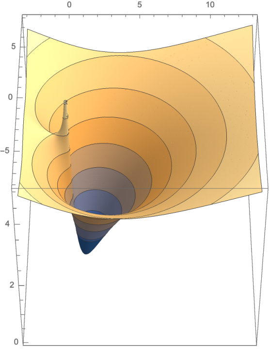
See Figure 3 for a plot of (the negative of)

We then recall that the function is a multiple of the Green’s function for the Laplacian on the plane, meaning that the function is harmonic away from the origin and that
where is a -measure at the origin. Thus, if we take the Laplacian of with an appropriate normalizing factor, we get the following nice result.
Proposition 5.
Recall that if is a strictly positive self-adjoint matrix, then we can take the logarithm of which is the self-adjoint matrix obtained by keeping the eigenvectors of fixed and taking the logarithm of the eigenvalues.
Proposition 6.
The function in (8) can also be computed as
| (9) |
or as
| (10) |
Here the logarithm is the self-adjoint logarithm of a positive self-adjoint matrix.
Note that in (9), the logarithm is undefined when is an eigenvalue of In (10), inserting guarantees that the logarithm is well defined for all but a singularity of at each eigenvalue still arises in the limit as approaches zero.
Proof.
An elementary result [24, Theorem 2.12] says that for any matrix we have . If is a strictly positive matrix, we may apply this result with (so that ) to get
or
Let us now apply this identity with whenever is not an eigenvalue of to obtain
where this last expression is the definition of
Continuity of the matrix logarithm then establishes (10). ∎
3.3. Definition and basic properties
To define the Brown measure of a general element in a tracial von Neumann algebra we use the obvious generalization of (10). We refer to Brown’s original paper [7] along with Chapter 11 of [34] for general references on the material in this section.
Theorem 7.
Let be a tracial von Neumann algebra and let be an arbitrary element of Define
| (11) |
for all and Then
| (12) |
exists as an almost-everywhere-defined subharmonic function. Furthermore, the quantity
| (13) |
where the Laplacian is computed in the distribution sense, is represented by a probability measure on the plane. We call this measure the Brown measure of and denote it by
The Brown measure of is supported on the spectrum of and has the property that
| (14) |
for all non-negative integers
See the original article [7] or Chapter 11 of the monograph [34] of Mingo and Speicher. We also note that the quantity is the logarithm of the Fuglede–Kadison determinant of ; see [13, 14]. It is important to emphasize that, in general, the moment condition (14) does not uniquely determine the measure After all, is an arbitrary nonempty compact subset of which could, for example, be a closed disk. To uniquely determine the measure, we would need to know the value of for all non-negative integers and There is not, however, any simple way to compute the value of in terms of the operator . In particular, unless is normal, this integral need not be equal to Thus, to compute the Brown measure of a general operator we actually have to work with the rather complicated definition in (11), (12), and (13).
We note two important special cases.
- •
Suppose is the space of all matrices and is the normalized trace, Then the Brown measure of any is simply the empirical eigenvalue distribution of which puts mass at each eigenvalue of
- •
If is normal, then the Brown measure of agrees with the measure defined in (7) using the spectral theorem.
3.4. Brown measure in random matrix theory
Suppose one has a family of random matrix models and one wishes to determine the large- limit of the empirical eigenvalue distribution of (Recall Definition 1.) One may naturally use the following three-step process.
Step 1. Construct a large- limit of as an operator in a tracial von Neumann algebra
Step 2. Determine the Brown measure of
Step 3. Prove that the empirical eigenvalue distribution of converges almost surely to as tends to infinity.
It is important to emphasize that Step 3 in this process is not automatic. Indeed, this can be a difficult technical problem. Nevertheless, this article is concerned with exclusively with Step 2 in the process (in situations where Step 1 has been carried out). For Step 3, the main tool is the Hermitization method developed in Girko’s pioneering paper [16] and further refined by Bai [1]. (Although neither of these authors explicitly uses the terminology of Brown measure, the idea is lurking there.)
There exist certain pathological examples where the limiting eigenvalue distribution does not coincide with the Brown measure. In light of a result of Śniady [38], we can say that such examples are associated with spectral instability, that is, matrices where a small change in the matrix produces a large change in the eigenvalues. Śniady shows that if we add to a small amount of random Gaussian noise, then eigenvalues distribution of the perturbed matrices will converge to the Brown measure of the limiting object. (See also the papers [19] and [12], which obtain similar results by very different methods.) Thus, if the original random matrices are somehow “stable,” adding this noise should not change the eigenvalues of by much, and the eigenvalues of the original and perturbed matrices should be almost the same. In such a case, we should get convergence of the eigenvalues of to the Brown measure of the limiting object.
The canonical example in which instability occurs is the case in which the deterministic matrix having ’s just above the diagonal and 0’s elsewhere. Then of course is nilpotent, so all of its eigenvalues are zero. We note however, that both and are diagonal matrices whose diagonal entries have values of 1 and only a single value of 0. Thus, when is large, is “almost unitary,” in the sense that and are close to the identity. Furthermore, for any positive integer we have that is again nilpotent, so that Using these observations, it is not hard to show that the limiting object is a “Haar unitary,” that is, a unitary element of a tracial von Neumann algebra satisfying for all positive integers The Brown measure of a Haar unitary is the uniform probability measure on the unit circle, while of course the eigenvalue distribution is entirely concentrated at the origin.
In Figure 4 we see that even under a quite small perturbation (adding times a Ginibre matrix), the spectrum of the nilpotent matrix changes quite a lot. After the perturbation, the spectrum clearly resembles a uniform distribution over the unit circle. In Figure 5, by contrast, we see that even under a much larger perturbation (adding times a Ginibre matrix), the spectrum of a GUE matrix changes only slightly. (Note the vertical scale in Figure 5.)
3.5. The case of the circular Brownian motion
We now record the Brown measure of the circular Brownian motion.
Proposition 8.
For any the Brown measure of is the uniform probability measure on the disk of radius centered at the origin.
Now, as we noted in Section 2.4, the -distribution of the circular Brownian motion at any time is the same as the -distribution of Thus, the proposition will follow if we know that the Brown measure of a circular element is the uniform probability measure on the unit disk. This result, in turn, is well known; see, for example, Section 11.6.3 of [34].
4. PDE for the circular law
The PDE methods developed in [10] were extended by Ho and Zhong [29] to the case of a free multiplicative Brownian motion with an arbitrary unitary initial distribution. Ho and Zhong also analyze [29, Section 3] the case of the free circular Brownian motion with an arbitrary self-adjoint initial condition. In this article, I explain how the proof in [29] works in the very special case of the free circular Brownian motion with an initial condition of 0.
The significance of this analysis is not so much that it gives another computation of the Brown measure of a circular element. Rather, it is a helpful warm-up case on the path to tackling more complicated problems, such as those in [10] and [29]. In this section and the two that follow, I will show how the PDE method applies in the case of the circular Brownian motion. Then in the last section, I will outline the case of the free multiplicative Brownian motion, leaving the details to [10].
We let be the circular Brownian motion (Section 2.4). Then, following the construction of the Brown measure in Theorem 7, we define, for each a function given by
| (15) |
for all and The Brown measure of will then be obtained by letting tend to zero, taking the Laplacian with respect to and dividing by The first main result—following [29, Section 3]—is that, for each satisfies a PDE in and
Theorem 9.
For each the function satisfies the first-order, nonlinear differential equation
| (16) |
subject to the initial condition
This result (with a more general initial condition) was established in Proposition 3.1 of [29]. We may now see the motivation for making a parameter rather than a variable for : since does not appear in the PDE (16), we can think of solving the same equation for each different value of with the dependence on entering only through the initial conditions.
On the other hand, we see that the regularization parameter plays a crucial role here as one of the variables in our PDE. Of course, we are ultimately interested in letting tend to zero, but since derivatives with respect to appear, we cannot merely set in the PDE.
Of course, the reader will point out that, formally, setting in (16) gives because of the leading factor of on the right-hand side. This conclusion, however, is not actually correct, because can blow up as approaches zero. Actually, it will turn out that is independent of when but not in general.
4.1. The finite- equation
In this subsection, we give a heuristic argument for the PDE in Theorem 9. Although the argument is not rigorous as written, it should help explain what is going on. In particular, the computations that follow should make it clear why the PDE is only valid after taking the large- limit.
4.1.1. The result
We introduce a finite- analog of the function in Theorem 9 and compute its time derivative. Let denote the Ginibre Brownian motion introduced in Section 1.3.
Proposition 10.
For each let
Then we have the following results.
- (1)
The time derivative of may be computed as
(17) - (2)
We also have
(18) - (3)
Therefore, if we set
we may rewrite the formula for as
(19) where is a “variance term” given by
The key point to observe here is that in the formula (17) for , we have the expectation value of the square of a trace. On the other hand, if we computed by taking the expectation value of both sides of (18) and squaring, we would have the square of the expectation value of a trace. Thus, there is no PDE for —we get an unavoidable covariance term on the right hand side of (19).
On the other hand, the Ginibre Brownian motion exhibits a concentration phenomenon for large Specifically, let us consider a family of random variables of the form
(Thus, for example, we might have ) Then it is known that (1) the large- limit of exists, and (2) the variance of goes to zero. That is to say, when is large, will be, with high probability, close to its expectation value. It then follows that will be close to (This concentration phenomenon was established by Voiculescu in [42] for the analogous case of the “GUE Brownian motion.” The case of the Ginibre Brownian motion is similar.)
Now, although the quantity
is not a word in and it is expressible—at least for large —as a power series in such words. It is therefore reasonable to expect—this is not a proof!—that the variance of will go to zero as goes to infinity, and the variance term in (19) will vanish in the limit.
4.1.2. Setting up the computation
We view as a real vector space of dimension and we use the following real-valued inner product :
| (20) |
The distribution of is the Gaussian measure of variance with respect to this inner product
where is a normalization constant and is the Lebesgue measure on This measure is a heat kernel measure. If we let denote the expectation value with respect to then we have, for any “nice” function,
| (21) |
where is the Laplacian on with respect to the inner product (20).
To compute more explicitly, we choose an orthonormal basis for over consisting of and where are skew-Hermitian and where We then introduce the directional derivatives and defined by
Then the Laplacian is given by
We also introduce the corresponding complex derivatives, and given by
which give
We now let denote a matrix-valued variable ranging over We may easily compute the following basic identities:
| (22) |
(Keep in mind that is skew-Hermitian.) We will also need the following elementary but crucial identity
| (23) |
where is the normalized trace, given by
See, for example, Proposition 3.1 in [9]. When applied to function involving a normalized trace, this will produce second trace.
Finally, we need the following formulas for differentiating matrix-valued functions of a real variable:
| (24) | ||||
| (25) |
The first of these is standard and can be proved by differentiating the identity The second identity is Lemma 1.1 in [7]; it is important to emphasize that this second identity does not hold as written without the trace. One may derive (25) by using an integral formula for the derivative of the logarithm without the trace (see, for example, Equation (11.10) in [27]) and then using the cyclic invariance of the trace, at which point the integral can be computed explicitly.
4.1.3. Proof of Proposition 10
We continue to let denote the expectation value with respect to the measure which is the distribution at time of the Ginibre Brownian motion so that
where the variable ranges over We apply the derivative using (25) and (22), giving
We then apply the derivative using (24) and (22), giving
We now sum on and apply the identity (23). After applying the heat equation (21) with we obtain
| (26) |
4.2. A derivation using free stochastic calculus
4.2.1. Ordinary stochastic calculus
In this section, I will describe briefly how the PDE in Theorem 9 can be derived rigorously, using the tools of free stochastic calculus. The proof will follow Section 3 of [29].
We begin by recalling a little bit of ordinary stochastic calculus, for the ordinary, real-valued Brownian motion. To avoid notational conflicts, we will let denote Brownian motion in the real line. This is a random continuous path satisfying the properties proposed by Einstein in 1905, namely that for any the increments
should be independent normal random variables with mean zero and variance At a rigorous level, Brownian motion is described by the Wiener measure on the space of continuous paths.
It is a famous result that, with probability one, the path is nowhere differentiable. This property has not, however, deterred people from developing a theory of “stochastic calculus” in which one can take the “differential” of denoted (Since is not differentiable, we should not attempt to rewrite this differential as ) There is then a theory of “stochastic integrals,” in which one can compute, for example, integrals of the form
where is some smooth function.
A key difference between ordinary and stochastic integration is that is not negligible compared to To understand this assertion, recall that the increments of Brownian motion have variance —and therefore standard deviation This means that in a short time interval the Brownian motion travels distance roughly Thus, if we may say that Thus, if is a smooth function, we may use a Taylor expansion to claim that
We may express the preceding discussion in the heuristically by saying
Rigorously, this line of reasoning lies behind the famous Itô formula, which says that
The formula means, more precisely, that (after integration)
where the first integral on the right-hand side is a stochastic integral and the second is an ordinary Riemann integral.
If we take, for example, then we find that
so that
This formula differs from what we would get if were smooth by the term on the right-hand side.
4.2.2. Free stochastic calculus
We now turn to the case of the circular Brownian motion Since is a limit of ordinary Brownian motion in the space of matrices, we expect that will be non-negligible compared to The rules are as follows; see [31, Lemma 2.5, Lemma 4.3]. Suppose and are processes “adapted to ,” meaning that and belong to the von Neumann algebra generated by the operators with Then we have
| (27) | ||||
| (28) | ||||
| (29) |
In addition, we have the following Itô product rule: if are processes adapted to , then
| (30) | ||||
| (31) |
Finally, the differential “” can be moved inside the trace
4.2.3. The proof
In the proof that follows, the Itô formula (27) plays the same role as the identity (23) plays in the heuristic argument in Section 4.1. We begin with a lemma whose proof is an exercise in using the rules of free stochastic calculus.
Lemma 11.
For each let us use the the notation
Then for each positive integer we have
Proof.
We first note that and since is a constant. We then compute by moving the inside the trace and then applying the product rule in (30) and (31). By (29), the terms arising from (30) will not contribute. Furthermore, by (28), the only terms from (31) that contribute are those where one goes on a factor of and one goes on a factor of
By choosing all possible factors of and all possible factors of we get terms. In each term, after putting the inside the trace, we can cyclically permute the factors until, say, the factor is at the end. There are then only distinct terms that occur, each of which occurs times. By (27), each distinct term is computed as
Since each distinct term occurs times, we obtain
which is equivalent to the claimed formula. ∎
We are now ready to give a rigorous argument for the PDE.
Proof of Theorem 9.
We continue to use the notation We first compute, using the operator version of (25), that
| (32) |
We note that the definition of in (15) actually makes sense for all with using the standard branch of the logarithm function. We note that for we have
| (33) |
Integrating with respect to gives
Thus, for we have
| (34) |
Assume for the moment that it is permissible to differentiate (34) term by term with respect to Then by Lemma 11, we have
| (35) |
Now, by [5, Proposition 3.2.3], the map is continuous in the operator norm topology; in particular, is a locally bounded function of From this observation, it is easy to see that the right-hand side of (35) converges locally uniformly in Thus, a standard result about interchange of limit and derivative (e.g., Theorem 7.17 in [37]) shows that the term-by-term differentiation is valid.
Now, in (35), we let and so that Then and go from 0 to and we get
(We may check that the power of in the denominator is and that the power of is ) Thus, moving the sums inside the traces and using (33), we obtain that
| (36) |
which reduces to the claimed PDE for by (32).
We have now established the claimed formula for for in the right half-plane, provided is sufficiently large, depending on and Since, also, we have, for sufficiently large
| (37) |
We now claim that both sides of (37) are well-defined, holomorphic functions of for in the right half-plane. This claim is easily established from the standard power-series representation of the inverse:
and a similar power-series representation of the logarithm. Thus, (37) actually holds for all in the right half-plane. Differentiating with respect to then establishes the desired formula (36) for for all in the right half-plane. ∎
5. Solving the equation
5.1. The Hamilton–Jacobi method
The PDE (16) in Theorem 9 is a first-order, nonlinear equation of Hamilton–Jacobi type. “Hamilton–Jacobi type” means that the right-hand side of the equation involves only and and not itself. The reader may consult Section 3.3 of the book [11] of Evens for general information about equations of this type. In this subsection, we describe the general version of this method. In the remainder of this section, we will then apply the general method to the PDE (16).
The Hamilton–Jacobi method for analyzing solutions to equations of this type is a generalization of the method of characteristics. In the method of characteristics, one finds certain special curves along which the solution is constant. For a general equation of Hamilton–Jacobi type, the method of characteristics in not applicable. Nevertheless, we may hope to find certain special curves along which the solution varies in a simple way, allowing us to compute the solution along these curves in a more-or-less explicit way.
We now explain the representation formula for solutions of equations of Hamilton–Jacobi type. A self-contained proof of the following result is given as the proof of Proposition 6.3 in [10].
Proposition 12.
Fix a function defined for in an open set and in Consider a smooth function on satisfying
| (38) |
for and Now suppose is curve in satisfying Hamilton’s equations:
with initial conditions
| (39) |
Then we have
| (40) |
and
| (41) |
We emphasize that we are not using the Hamilton–Jacobi formula to construct a solution to the equation (38); rather, we are using the method to analyze a solution that is assumed ahead of time to exist. Suppose we want to use the method to compute (as explicitly as possible), the value of for some fixed We then need to try to choose the initial position in (39)—which determines the initial momentum —so that We then use (40) to get an in-principle formula for
5.2. Solving the equations
The equation for in Theorem 9 is of Hamilton–Jacobi form with , with Hamiltonian given by
| (42) |
Since is only defined for we take open set in Proposition 12 to be That is to say, the Hamilton–Jacobi formula (40) is only valid if the curve remains positive for
Hamilton’s equations for this Hamiltonian then take the explicit form
| (43) | ||||
| (44) |
Following the general method, we take an arbitrary initial position , with the initial momentum given by
| (45) |
Theorem 13.
Proof.
Since the equation (44) for does not involve we may easily solve it for as
We may then plug the formula for into the equation (43) for giving
so that
Thus,
so that
Plugging in gives Recalling the expression (45) for gives the claimed formula for
6. Letting tend to zero
Recall that the Brown measure is obtained by first evaluating
and then taking times the Laplacian (in the distribution sense) of We record the result here and will derive it in the remainder of this section.
Theorem 14.
We have
| (48) |
The Brown measure is then absolutely continuous with respect to the Lebesgue measure, with density given by
| (49) |
That is to say, the Brown measure is the uniform probability measure on the disk of radius centered at the origin. The functions and are plotted for in Figure 6. On the left-hand side of the figure, the dashed line indicates the boundary of the unit disk.

6.1. Letting tend to zero: outside the disk
Our goal is to compute . Thus, in the Hamilton–Jacobi formalism, we want to try to choose so that the quantity
| (50) |
will be very close to zero. Since there is a factor of on the right-hand side of the above formula, an obvious strategy is to take itself very close to zero. There is, however, a potential difficulty with this strategy: If is small, the lifetime of the solution may be smaller than the time we are interested in. To see when the strategy works, we take the formula for the lifetime of the solution—namely —and take the limit as tends to zero.
Definition 15.
Thus, if the time we are interested in is larger than our simple strategy of taking will not work. After all, if and then the lifetime of the path is less than and the Hamilton–Jacobi formula (47) is not applicable. On the other hand, if the time we are interested in is at most the simple strategy does work. Figure 7 illustrates the situation.
Conclusion 16.
The simple strategy of letting approach zero works precisely when Equivalently, the simple strategy works when that is, when is outside the open disk of radius centered at the origin.
In the case that is outside the disk, we may then simply let approach zero in the Hamilton–Jacobi formula, giving the following result.
Proposition 17.
Suppose that is, that is outside the open disk of radius centered at 0. Then we may let tend to zero in the Hamilton–Jacobi formula (47) to obtain
| (51) |
Since the right-hand side of (51) is harmonic, we conclude that
That is to say, the Brown measure of is zero outside the disk of radius centered at 0.
6.2. Letting tend to zero: inside the disk
We now turn to the case in which the time we are interested in is greater than the small- lifetime of the solutions to (43)–(44). This case corresponds to that is, We still want to choose so that will approach zero, but we cannot let tend to zero, or else the lifetime of the solution will be less than Instead, we allow the second factor in the formula (46) for to approach zero. To make this factor approach zero, we make approach that is, should approach Note that since we are now assuming that the quantity is positive. This strategy is illustrated in Figure 8: When we obtain and if approaches from above, the value of approaches 0 from above.
Proposition 18.
Suppose that is, that is inside the closed disk of radius centered at 0. Then in the Hamilton–Jacobi formula (47), we may let approach from above, and we get
For we may then compute
Thus, inside the disk of radius the Brown measure has a constant density of
Proof.
6.3. On the boundary
Note that if both approaches are valid—and the two values of agree, with a common value of Furthermore, the radial derivatives of agree on the boundary: on the outside and on the inside, which have a common value of at Of course, the angular derivatives of are identically zero, inside, outside, and on the boundary.
Since the first derivatives of are continuous up to the boundary, we may take the distributional Laplacian by taking the ordinary Laplacian inside the disk and outside the disk and ignoring the boundary. (See the proof of Proposition 7.13 in [10].) Thus, we may compute the Laplacian of the two formulas in (48) to obtain the formula (49) for the Brown measure of
7. The case of the free multiplicative Brownian motion
7.1. Additive and multiplicative models
The standard GUE and Ginibre ensembles are given by Gaussian measures on the relevant space of matrices (Hermitian matrices for GUE and all matrices for the Ginibre ensemble). In light of the central limit theorem, these ensembles can be approximated by adding together large numbers of small, independent random matrices. We may therefore refer to these Gaussian ensembles as “additive” models.
It is natural to consider also “multiplicative” random matrix models, which can be approximated by multiplying together large numbers of independent matrices that are “small” in the multiplicative sense, that is, close to the identity. Specifically, if is a random matrix with a Gaussian distribution, we will consider a multiplicative version where the distribution of may be approximated as
| (52) |
Here is a positive parameter, the ’s are independent copies of and “Itô” is an Itô correction term. This correction term is a fixed multiple of the identity, independent of and (In the next paragraph, we will identify the Itô term in the main cases of interest.) Since the factors in (52) are independent and identically distributed, the order of the factors does not affect the distribution of the product.
The two main cases we will consider are those in which is distributed according to the Gaussian unitary ensemble or the Ginibre ensemble. In the case that is distributed according to the Gaussian unitary ensemble, the Itô term is In this case, the resulting multiplicative model may be described as Brownian motion in the unitary group which we write as The Itô correction is essential in this case to ensure that actually lives in the unitary group. In the case that is distributed according to the Ginibre ensemble, the Itô term is zero. In this case, the resulting multiplicative model may be described as Brownian motion in the general linear group , which we write as
7.2. The free unitary and free multiplicative Brownian motions
The large- limits of the Brownian motions and were constructed by Biane [3]. The limits are the free unitary Brownian motion and the free multiplicative Brownian motion, respectively, which we write as and The qualifier “free” indicates that the increments of these Brownian motions—computed in the multiplicative sense as or —are freely independent in the sense of Section 2.3. In the case of the convergence of to was conjectured by Biane [3] and proved by Kemp [31]. In both cases, we take the limiting object to be an element of a tracial von Neumann algebra
Since is unitary, we do not need to use the machinery of Brown measure, but can rather use the spectral theorem as in (7) to compute the distribution of denoted We emphasize that is, in fact, the Brown measure of but it easier to describe using the spectral theorem than to use the general Brown measure construction. The measure is a probability measure on the unit circle describing the large- limit of Brownian motion in the unitary group Biane computed the measure in [3] and established the following support result.
Theorem 19.
For the measure is supported on a proper subset of the unit circle:
By contrast, for all the closed support of is the whole unit circle.
In the physics literature, the change in behavior of the support of at is called a topological phase transition, indicating that the topology of changes from a closed interval to a circle.
The remainder of this article is devoted to recent results of the author with Driver and Kemp regarding the Brown measure of the free multiplicative Brownian motion We expect that the Brown measure of will be the limiting empirical eigenvalue distribution of the Brownian motion in the general linear group . Now, when is small, we may take in (52), so that (since the Itô correction is zero in this case),
Thus, when is small and is large, the eigenvalues of resemble a scaled and shifted version of the circular law. Specifically, the eigenvalue distribution should resemble a uniform distribution on the disk of radius centered at 1.
Figure 9 shows the eigenvalues of with and The eigenvalue distribution bears a clear resemblance to the just-described picture, with Nevertheless, we can already see some deviation from the small- picture: The region into which the eigenvalues are clustering looks like a disk, but not quite centered at 1, while the distribution within the region is slightly higher at the left-hand side of the region than the right. Figures 10 and 11, meanwhile, show the eigenvalue distribution of for several larger values of The region into which the eigenvalues cluster becomes more complicated as increases, and the distribution of eigenvalues in the region becomes less and less uniform. We expect that the Brown measure of the limiting object will be supported on the domain into which the eigenvalues are clustering.
7.3. The domains
We now describe certain domains in the plane, as introduced by Biane in [4, pp. 273-274]. It will turn out that the Brown measure of is supported on We use here a new the description of as given in Section 4 of [10]. For all nonzero we define
| (53) |
If we interpret as having the value 1 when in accordance with the limit
See Figure 12 for a plot of this function.
We then define the domains as follows.
Definition 20.
For each we define
Several examples of these domains were plotted already in Figures 9, 10, and 11. The domain is simply connected for and doubly connected for The change in behavior at occurs because has a saddle point at and because We note that a change in the topology of the region occurs at which is the same value of at which the topology of the support of Biane’s measure changes (Theorem 19).
7.4. The support of the Brown measure of
As we have noted, the domains were introduced by Biane in [4]. Two subsequent works in the physics literature, the article [18] by Gudowska-Nowak, Janik, Jurkiewicz, and Nowak and the article [32] by Lohmayer, Neuberger, and Wettig then argued, using nonrigorous methods, that the eigenvalues of should concentrate into for large The first rigorous result in this direction was obtained by the author with Kemp [26]; we prove that the Brown measure of is supported on the closure of
Now, we have already noted that is simply connected for but doubly connected for Thus, the support of the Brown measure of the free multiplicative Brownian motion undergoes a “topological phase transition” at precisely the same value of the time-parameter as the distribution of the free unitary Brownian motion (Theorem 19).
The methods of [26] explain this apparent coincidence, using the “free Hall transform” of Biane [4]. Biane constructed this transform using methods of free probability as an infinite-dimensional analog of the Segal–Bargmann transform for which was developed by the author in [21]. More specifically, Biane’s definition draws on the stochastic interpretation of the transform in [21] given by Gross and Malliavin [17]. Biane conjectured (with an outline of a proof) that is actually the large- limit of the transform in [21]. This conjecture was then verified by in independent works of Cébron [8] and the author with Driver and Kemp [9]. (See also the expository article [25].)
Recall from Section 7.2 that the distribution of the free unitary Brownian motion is Biane’s measure on the unit circle, the support of which is described in Theorem 19. A key ingredient in [26] is the function given by
| (54) |
This function maps the complement of the closure of conformally to the complement of the support of Biane’s measure:
| (55) |
(This map will also play a role in the results of Section 7.5; see Theorem 23.)
The key computation in [26] is that for outside we have
| (56) |
See Theorem 6.8 in [26]. Properties of the free Hall transform then imply that for outside the operator has an inverse. Indeed, the noncommutative norm of equals to the norm in of the function on the right-hand side of (56). This norm, in turn, is finite because is outside the support of whenever is outside The existence of an inverse to then shows that must be outside the support of
An interesting aspect of the paper [26] is that we not only compute the support of but also that we connect it to the support of Biane’s measure using the transform and the conformal map
7.5. The Brown measure of
We now describe the main results of [10]. Many of these results have been extended by Ho and Zhong [29] to the case of the free multiplicative Brownian motion with an arbitrary unitary initial distribution.
The first key result in [10] is the following formula for the Brown measure of (Theorem 2.2 of [10]).
Theorem 21.
For each the Brown measure is zero outside the closure of the region In the region the Brown measure has a density with respect to Lebesgue measure. This density has the following special form in polar coordinates:
for some positive continuous function The function is determined entirely by the geometry of the domain and is given as
where is the “outer radius” of the region at angle
See Figure 13 for the definition of Figure 14 for plots of the function , and Figure 15 for a plot of The simple explicit dependence of on is a major surprise of our analysis. See Corollary 22 for a notable consequence of the form of
Using implicit differentiation, it is possible to compute explicitly as a function of This computation yields the following formula for which does not involve differentiation:
where
| (57) |
and
See Proposition 2.3 in [10].

We expect that the Brown measure of will coincide with the limiting empirical eigenvalue distribution of the Brownian motion in This expectation is supported by simulations; see Figure 16.

We note that the Brown measure (inside ) can also be written as
Since the complex logarithm is given by we obtain the following consequence of Theorem 21.
Corollary 22.
The push-forward of the Brown measure under the complex logarithm has density that is constant in the horizontal direction and given by in the vertical direction.
In light of this corollary, we expect that for large the logarithms of the eigenvalues of should be approximately uniformly distributed in the horizontal direction. This expectation is confirmed by simulations, as in Figure 17.
We conclude this section by describing a remarkable connection between the Brown measure and the distribution of the free unitary Brownian motion. Recall the holomorphic function in (54) and (55). This map takes the boundary of to the unit circle. We ma then define a map
by requiring (a) that should agree with on the boundary of and (b) that should be constant along each radial segment inside as in Figure 18. (This specification makes sense because has the same value at the two boundary points on each radial segment.) We then have the following result, which may be summarized by saying that the distribution of free unitary Brownian motion is a “shadow” of the Brown measure of .
Theorem 23.
The push-forward of the Brown measure of under the map is Biane’s measure on Indeed, the Brown measure of is the unique measure on with the following two properties: (1) the push-forward of by is and (2) is absolutely continuous with respect to Lebesgue measure with a density having the form
in polar coordinates, for some continuous function
This result is Proposition 2.6 in [10]. Figure 19 shows the eigenvalues for after applying the map plotted against the density of Biane’s measure We emphasize that we have computed the eigenvalues of the Brownian motion in (in the two-dimensional region ) and then mapped these points to the unit circle. The resulting histogram, however, looks precisely like a histogram of the eigenvalues of the Brownian motion in
7.6. The PDE and its solution
We conclude this article by briefly outlining the methods used to obtain the results in the previous subsection.
7.6.1. The PDE
Following the definition of the Brown measure in Theorem 7, we consider the function
| (58) |
We then record the following result [10, Theorem 2.8].
Theorem 24.
Recall that in the case of the circular Brownian motion (the PDE in Theorem 9), the complex number enters only into the initial condition and not into the PDE itself. By contrast, the right-hand side of the PDE (59) involves differentiation with respect to the real and imaginary parts of
On the other hand, the PDE (59) is again of Hamilton–Jacobi type. Thus, following the general Hamilton–Jacobi method in Section 5.1, we define a Hamiltonian function from (the negative of) the right-hand side of (59), replacing each derivative of by a corresponding momentum variable:
| (61) |
We then consider Hamilton’s equations for this Hamiltonian:
| (62) |
Then, after a bit of simplification, the general Hamilton–Jacobi formula in (40) then takes the form
| (63) |
(See Theorem 6.2 in [10].)
The analysis in [10] then proceeds along broadly similar lines to those in Sections 5 and 6. The main structural difference is that because is now a variable in the PDE, the ODE’s in (62) now involve both and and the associated momenta. (That is to say, the vector in Proposition 12 is equal to ) The first key result is that the system of ODE’s associated to (59) can be solved explicitly; see Section 6.3 of [10]. Solving the ODE’s gives an implicit formula for the solution to (59) with the initial conditions (60).
We then evaluate the solution in the limit as tends to zero. We follow the strategy in Section 6. Given a time and a complex number we attempt to choose initial conditions and so that will be very close to zero and will equal (Recall that the initial momenta in the system of ODE’s are determined by the positions by (39).)
7.6.2. Outside the domain
As in the case of the circular Brownian motion, we use different approaches for outside and for in For outside we allow the initial condition in the ODE’s to approach zero. As it turns out, when is small and positive, remains small and positive for as long as the solution to the system exists. Furthermore, when is small and positive, is approximately constant. Thus, our strategy will be to take and
A key result is the following.
Proposition 25.
This result is Proposition 6.13 in [10]. Thus, the strategy in the previous paragraph will work—meaning that the solution continues to exist up to time —provided that is greater than The condition for success of the strategy is, therefore, In light of the characterization of in Definition 20, we make have the following conclusion.
Conclusion 26.
The simple strategy of taking and is successful precisely if or equivalently, if is outside
When this strategy works, we obtain a simple expression for by letting approach zero and approach in (63). Since approaches in this limit [10, Proposition 6.11], we find that
| (64) |
This function is harmonic (except at which is always in the domain ), so we conclude that the Brown measure of is zero outside See Section 7.2 in [10] for more details.
7.6.3. Inside the domain
For inside the simple approach in the previous subsection does not work, because when is outside and is small, the solutions to the ODE’s (62) will cease to exist prior to time (Proposition 25). Instead, we must prove a “surjectivity” result: For each and there exist—in principle— and giving and See Figure 20. Actually the proof shows that again belongs to the domain ; see Section 6.5 in [10].

We then make use of the second Hamilton–Jacobi formula (41), which allows us to compute the derivatives of directly, without having to attempt to differentiate the formula (63) for Working in logarithmic polar coordinates, and we find an amazingly simple expression for the quantity
inside namely,
| (65) |
(See Corollary 7.6 in [10].) This result is obtained using a certain constant of motion of the system of ODE’s, namely the quantity
in [10, Proposition 6.5].
If we evaluate this constant of motion at a time when the term vanishes. But if the second Hamilton–Jacobi formula (41) tells us that
Furthermore, is just computed in rectangular coordinates. A bit of algebraic manipulation yields an explicit formula for as in [10, Theorem 6.7], explaining the formula (65). To complete the proof (65), it still remains to address certain regularity issues of near as in Section 7.3 of [10].
Once (65) is established, we note that the formula for in (65) is independent of It follows that
that is, that is independent of inside Writing the Laplacian in logarithmic polar coordinates, we then find that
| (66) |
where term in the expression comes from differentiating (65) with respect to Since is independent of we can understand the structure of the formula in Theorem 21.
The last step in the proof of Theorem 21 is to compute Since is independent of —or, equivalently, independent of —inside the value of at a point in is the same as its value as we approach the boundary of along the radial segment through We show that is continuous over the whole complex plane, even at the boundary of (See Section 7.4 of [10].) Thus, on the boundary of the function will agree with the angular derivative of , namely
| (67) |
Thus, to compute at a point in we simply evaluate (67) at either of the two points where the radial segment through intersects (We get the same value at either point.)
References
- [1] Z. D. Bai, Circular law, Ann. Probab. 25 (1997), 494–529.
- [2] P. Biane, On the free convolution with a semi-circular distribution, Indiana Univ. Math. J. 46 (1997), 705–718.
- [3] P. Biane, Free Brownian motion, free stochastic calculus and random matrices. In Free Probability Theory (Waterloo, ON, 1995), 1–19. Fields Institute Communications 12. Providence, RI: American Mathematical Society, 1997.
- [4] P. Biane, Segal–Bargmann transform, functional calculus on matrix spaces and the theory of semi-circular and circular systems, J. Funct. Anal. 144 (1997), 232–286.
- [5] P. Biane and R. Speicher, Stochastic calculus with respect to free Brownian motion and analysis on Wigner space, Probab. Theory Related Fields 112 (1998), 373–409.
- [6] P. Bourgade and J. P. Keating, Quantum chaos, random matrix theory, and the Riemann -function. In Chaos, 125–168, Prog. Math. Phys., 66, Birkhäuser/Springer, Basel, 2013.
- [7] Brown, L. G. Lidskiĭ’s theorem in the type II case. In Geometric methods in operator algebras (Kyoto, 1983), 1–35, Pitman Res. Notes Math. Ser., 123, Longman Sci. Tech., Harlow, 1986.
- [8] G. Cébron, Free convolution operators and free Hall transform, J. Funct. Anal. 265 (2013), 2645–2708.
- [9] B. K. Driver, B. C. Hall, and T. Kemp, The large- limit of the Segal–Bargmann transform on , J. Funct. Anal. 265 (2013), 2585–2644.
- [10] B. K. Driver, B. C. Hall, and T. Kemp, The Brown measure of the free multiplicative Brownian motion, preprint arXiv:1903.11015 [math.PR].
- [11] L. C. Evans, Partial differential equations. Second edition. Graduate Studies in Mathematics, 19. American Mathematical Society, Providence, RI, 2010. xxii+749 pp.
- [12] O. Feldheim, E. Paquette, and O. Zeitouni, Regularization of non-normal matrices by Gaussian noise, Int. Math. Res. Not. IMRN 18 (2015), 8724–8751.
- [13] B. Fuglede and R. V. Kadison, On determinants and a property of the trace in finite factors, Proc. Nat. Acad. Sci. U. S. A. 37 (1951), 425–431.
- [14] B. Fuglede and R. V. Kadison, Determinant theory in finite factors, Ann. of Math. (2) 55 (1952), 520–530.
- [15] J. Ginibre, Statistical ensembles of complex, quaternion, and real matrices, J. Math. Phys. 6 (1965), 440–449.
- [16] V. L. Girko, The circular law. (Russian) Teor. Veroyatnost. i Primenen. 29 (1984), 669–679.
- [17] L. Gross and P. Malliavin, Hall’s transform and the Segal–Bargmann map. In Itô’s stochastic calculus and probability theory (N. Ikeda, S. Watanabe, M. Fukushima and H. Kunita, Eds.), 73–116, Springer, 1996.
- [18] E. Gudowska-Nowak, R. A. Janik, J. Jurkiewicz, and M. A. Nowak, Infinite products of large random matrices and matrix-valued diffusion, Nuclear Phys. B 670 (2003), 479–507.
- [19] A. Guionnet, P. M. Wood, and O. Zeitouni, Convergence of the spectral measure of non-normal matrices, Proc. Amer. Math. Soc. 142 (2014), 667–679.
- [20] M. C. Gutzwiller, Chaos in classical and quantum mechanics. Interdisciplinary Applied Mathematics, 1. Springer-Verlag, New York, 1990.
- [21] B. C. Hall, The Segal–Bargmann “coherent state” transform for compact Lie groups. J. Funct. Anal. 122 (1994), 103–151.
- [22] B. C. Hall, Harmonic analysis with respect to heat kernel measure, Bull. Amer. Math. Soc. (N.S.) 38 (2001), 43–78.
- [23] B. C. Hall, Quantum theory for mathematicians. Graduate Texts in Mathematics, 267. Springer, New York, 2013.
- [24] B. C. Hall, Lie groups, Lie algebras, and representations. An elementary introduction. Second edition. Graduate Texts in Mathematics, 222. Springer, 2015.
- [25] B. C. Hall, The Segal–Bargmann transform for unitary groups in the large- limit, preprint arXiv:1308.0615 [math.RT].
- [26] B. C. Hall and T. Kemp, Brown measure support and the free multiplicative Brownian motion, Adv. Math. 355 (2019), article 106771, 36 pp.
- [27] N. J. Higham, Functions of matrices. Theory and computation. Society for Industrial and Applied Mathematics (SIAM), Philadelphia, PA, 2008.
- [28] C.-W. Ho, The two-parameter free unitary Segal-Bargmann transform and its Biane-Gross-Malliavin identification, J. Funct. Anal. 271 (2016), 3765–3817.
- [29] C.-W. Ho and P. Zhong, Brown Measures of free circular and multiplicative Brownian motions with probabilistic initial point, preprint arXiv:1908.08150 [math.OA].
- [30] N. M. Katz and P. Sarnak, Zeroes of zeta functions and symmetry, Bull. Amer. Math. Soc. (N.S.) 36 (1999), 1–26.
- [31] T. Kemp, The large- limits of Brownian motions on , Int. Math. Res. Not., (2016), 4012–4057.
- [32] R. Lohmayer, H. Neuberger, and T. Wettig, Possible large- transitions for complex Wilson loop matrices, J. High Energy Phys. 2008, no. 11, 053, 44 pp.
- [33] M. L. Mehta, Random matrices. Third edition. Pure and Applied Mathematics (Amsterdam), 142. Elsevier/Academic Press, Amsterdam, 2004
- [34] J. A. Mingo and R. Speicher, Free probability and random matrices. Fields Institute Monographs, 35. Springer, New York; Fields Institute for Research in Mathematical Sciences, Toronto, ON, 2017.
- [35] H. L. Montgomery, The pair correlation of zeros of the zeta function. Analytic number theory (Proc. Sympos. Pure Math., Vol. XXIV, St. Louis Univ., St. Louis, Mo., 1972), pp. 181–193. Amer. Math. Soc., Providence, R.I., 1973.
- [36] A. Nica and R. Speicher, Lectures on the combinatorics of free probability. London Mathematical Society Lecture Note Series, 335. Cambridge University Press, Cambridge, 2006.
- [37] W. Rudin, Principles of mathematical analysis. Third edition. International Series in Pure and Applied Mathematics. McGraw-Hill Book Co., New York-Auckland-Düsseldorf, 1976.
- [38] P. Śniady, Random regularization of Brown spectral measure, J. Funct. Anal. 193 (2002), 291–313.
- [39] H.-J. Stöckmann, Quantum chaos. An introduction. Cambridge University Press, Cambridge, 1999.
- [40] T. Tao, Topics in random matrix theory. Graduate Studies in Mathematics, 132. American Mathematical Society, Providence, RI, 2012.
- [41] D. Voiculescu, Symmetries of some reduced free product -algebras. In “Operator algebras and their connections with topology and ergodic theory (Buşteni, 1983),” 556–588, Lecture Notes in Math., 1132, Springer, Berlin, 1985.
- [42] D. Voiculescu, Limit laws for random matrices and free products, Invent. Math. 104 (1991), 201–220.
- [43] E. Wigner, Characteristic vectors of bordered matrices with infinite dimensions. Ann. of Math. (2) 62 (1955), 548–564.