A Fat boundary-type method for localized nonhomogeneous material problems

Alex Viguerie Thanks: Department of Civil Engineering and Architecture, University of Pavia, Pavia, PV 27100, Italy(alexander.viguerie@unipv.it). Ferdinando Auricchio Thanks: Department of Civil Engineering and Architecture, University of Pavia, Pavia, PV 27100, Italy (auricchio@unipv.it). Silvia Bertoluzza Thanks: CNR Imati Enrico Magenes, Pavia, PV 27100 , Italy (silvia.bertoluzza@imati.cnr.it)

Abstract

Problems with localized nonhomogeneous material properties arise frequently in many applications and are a well-known source of difficulty in numerical simulations. In certain applications (including additive manufacturing), the physics of the problem may be considerably more complicated in relatively small portions of the domain, requiring a significantly finer local mesh compared to elsewhere in the domain. This can make the use of a uniform mesh numerically unfeasible. While nonuniform meshes can be employed, they may be challenging to generate (particularly for regions with complex boundaries) and more difficult to precondition. The problem becomes even more prohibitive when the region requiring a finer-level mesh changes in time, requiring the introduction of refinement and derefinement techniques. To address the aforementioned challenges, we employ a technique related to the Fat boundary method [1, 2, 20] as a possible alternative. We analyze the proposed methodology from a mathematical point of view and validate our findings on two-dimensional numerical tests.

1 Introduction

Problems with localized nonhomogeneous material properties are of great interest in engineering [3, 4, 5, 8, 9, 10, 11, 12, 14, 15, 16, 22, 23, 24, 25, 26, 27]. In such problems, the varying physical properties between the different regions result in potentially large modeling differences. In many instances, a material which comprises a relatively small portion of the domain may feature significantly more complex physics and, therefore, it may require a higher mesh resolution than in the remainder of the domain. Common examples of such problems with high industrial interest are thermal problems in additive manufacturing (where the nonlinear phase transformation phenomena occur only along a thin strip on the top of the domain)[3, 10, 11, 12, 14, 15, 16, 22, 23, 24, 25, 26, 27], or fluid flow problems through immersed membranes (where the flow properties change inside a subregion of the domain) [17, 18, 19, 21]. A simple diagram of such a physical situation is shown in Fig. 1.

While using fine mesh throughout the whole domain may give an acceptable numerical solution, the computational cost of such an approach may be prohibitive. In contrast, a mesh that is coarse in one region and fine in another, while computationally more attractive, may be difficult to generate and is also known to cause difficulties with preconditioning [5, 6, 7, 13]. Additionally, in some instances the boundary of the subregion may be geometrically complicated, or may change in time, requiring frequent remeshing or the use of complicated local refinement and derefinement techniques [12, 15, 22, 23, 24, 27].

We decided to approach such problems adopting a different methodology inspired by the Fat boundary method (see [1, 2, 20]), an algorithm originally designed to handle geometries with holes in which generating conformal meshes is difficult. The Fat boundary method works by solving problems on different meshes and coupling the different solutions by the introduction of point forces within the domain. In the present work, we develop a related technique that allows us to solve problems with localized nonhomogeneous features by using two separate meshes. In regions that require a higher mesh resolution, we solve the problem on a fine separate mesh; then, as in the Fat boundary method, we reinsert this solution on the coarse mesh as a forcing term. This approach can be viewed as a generalization of the Fat boundary method, since the subregions are not holes in the geometry but areas in which the material properties differ.

Refer to caption — Figure 1: Example physical situation. The domain features and imposed flux along one region and imposed temperature on the others. The material properties differ within the domain.

We structure the paper as follows. We first introduce the model problems and derive split-problem formulations, in which we express the model problems (originally defined on a single mesh) as a pair of problems on two different meshes with coupling conditions. Next, we use the split formulation to naturally derive two-level methods at both the continuous and discrete levels. We then present numerical examples of the proposed approach for both steady and unsteady problems and discuss the results. We conclude by discussing points for further improvement and future research directions.

2 Problem Splitting

In the following we focus on steady and unsteady thermal problems, which are often characterized by the presence of local features, such as a nonhomogeneous material inclusion or local nonlinear phase transition phenomena. Accordingly, in this section we formally derive split formulations for the study of such problems. The proposed formulations will then naturally form the basis for the two-level algorithm presented later in the work.

We consider a domain $\Omega$ with a subregion $\Omega_{-}\subset\Omega$ , as shown in Fig 2. Letting $\Omega_{+}=\Omega\setminus\overline{\Omega}_{-}$ , $\gamma=\partial\Omega_{-}$ , and denoting the unknown temperature field as $u$ , the steady thermal problem is given by:

\displaystyle\begin{split}-\nabla\cdot\left(\beta\nabla u\right)&=f\quad\text{in }\Omega{\color[rgb]{0,0,0}\setminus\gamma}\\ u&=T_{0}\quad\text{on }\Gamma_{D}\\ \beta\frac{\partial u}{\partial\bm{n}}&=q\quad\text{on }\Gamma_{N}\\ {\color[rgb]{0,0,0}[\![\beta\nabla u\cdot\bm{n}]\!]}&{\color[rgb]{0,0,0}=0\quad\text{on }\gamma}\\ {\color[rgb]{0,0,0}[\![u]\!]}&{\color[rgb]{0,0,0}=0\quad\text{on }\gamma}\end{split}

(2.1)

with the unsteady variant defined as:

\displaystyle\begin{split}\rho\frac{\partial u}{\partial t}-\nabla\cdot\left(\beta\nabla u\right)&=f\quad\text{in }\Omega\times\left[t_{0},\,t_{end}\right]\\ u&=T_{0}\quad\text{on }\Gamma_{D}\times\left[t_{0},\,t_{end}\right]\\ \beta\frac{\partial u}{\partial\bm{n}}&=q(t)\quad\text{on }\Gamma_{N}\times\left[t_{0},\,t_{end}\right]\\ u&=u_{0}\quad\text{at }t=t_{0}{\color[rgb]{0,0,0}.}\\ {\color[rgb]{0,0,0}[\![\beta\nabla u\cdot\bm{n}]\!]}&{\color[rgb]{0,0,0}=0\quad\text{on }\gamma}\ \\ {\color[rgb]{0,0,0}[\![u]\!]}&{\color[rgb]{0,0,0}=0\quad\text{on }\gamma}\end{split}

(2.2)

where $\partial u\big/\partial\bm{n}$ denotes the normal derivative, $q$ is a heat flux, $[\![\cdot]\!]$ denotes the jump across $\gamma$ , $\beta$ denotes the heat conductivity, defined as:

\displaystyle\beta:=\begin{cases}\beta_{+}\quad\text{in }\Omega_{+}\\ \beta_{-}\quad\text{in }\Omega_{-}\end{cases},

(2.3)

and $\rho$ denotes the heat capacity, defined as:

\displaystyle\quad\rho:=\begin{cases}\rho_{+}\quad\text{in }\Omega_{+}\\ \rho_{-}\quad\text{in }\Omega_{-}\end{cases}

(2.4)

In general, $\beta_{+}$ , $\beta_{-}$ , $\rho_{+}$ and $\rho_{-}$ are functions of time and space. However, as the constant-coefficient case greatly simplifies the mathematical formulation and analysis of the method, we will start by considering this simpler but important case, providing a more general analysis in an appendix at end of the present work.

As the methods discussed here bear a strong relationship to the previously discussed Fat boundary method, we follow the same notation used in [1, 2, 20] and denote the trace of $H^{1}\left(\Omega\right)$ on $\gamma$ as $H^{1/2}\left(\gamma\right)$ , with the corresponding dual spaces given by $H^{-1}\left(\Omega\right)$ and $H^{-1/2}\left(\gamma\right)$ respectively.

For $\eta\in H^{-1/2}\left(\gamma\right)$ , we define $\eta\delta_{\gamma}\in H^{-1}\left(\Omega\right)=H^{1}(\Omega)^{\prime}$ as the linear functional such that:

\displaystyle\int_{\Omega}\left(\eta\delta_{\gamma}\right)w=\int_{\gamma}\eta w\quad\quad\forall w\in H^{1}\left(\Omega\right),

(2.5)

and, in the spirit of the Fat boundary method, we propose to split Problem (2.1) with constant $\beta_{+}$ and $\beta_{-}$ into two subproblems as follows:

\displaystyle\begin{split}-\nabla\cdot\left(\beta_{+}\nabla{u}\right)&=f\big|_{\Omega_{+}}+\frac{\beta_{+}}{\beta_{-}}f\big|_{\Omega_{-}}+\left[\beta_{+}\frac{\partial\widetilde{u}}{\partial\bm{n}}\delta_{\gamma}-\beta_{-}\frac{\partial\widetilde{u}}{\partial\bm{n}}\delta_{\gamma}\right]\text{ in }\Omega\\ {u}&=T_{0}\text{ on }\Gamma_{D}\\ \beta_{+}\frac{\partial{u}}{\partial\bm{n}}&=q\text{ on }\Gamma_{N}\end{split}

(2.6)

and

\displaystyle\begin{split}-\nabla\cdot\left(\beta_{-}\nabla\widetilde{u}\right)&=f\text{ in }\Omega_{-}\\ \widetilde{u}&=u\text{ on }\gamma.\end{split}

(2.7)

We now prove a theorem, stating the equivalence between the model Problem (2.1) and Problems (2.6) and (2.7):

Theorem 2.1.

A temperature distribution $u$ solves Problem (2.1) with constant $\beta_{+}$ and $\beta_{-}$ if and only if the corresponding solution pair $(u,\widetilde{u})$ solves Problems (2.6) and (2.7).

Proof.

Let $u$ be a solution of (2.1). Define $\widetilde{u}$ as:

\widetilde{u}:=u|_{\Omega_{-}}.

(2.8)

This of course implies:

\displaystyle-\nabla\cdot\left(\beta_{-}\nabla\widetilde{u}\right)

\displaystyle=f\text{ in }\Omega_{-}.

(2.9)

Then for $u\in H^{1}\left(\Omega\right)$ and $\varphi\in C_{0}^{\infty}\left(\Omega\right)$ :

\displaystyle\begin{split}\int_{\Omega}\beta\nabla{u}\cdot\nabla{\varphi}&=\int_{\Omega}\beta_{+}\nabla{u}\cdot\nabla{\varphi}-\int_{\Omega_{-}}\beta_{+}\nabla u\cdot\nabla\varphi+\int_{\Omega_{-}}\beta_{-}\nabla u\cdot\nabla\varphi\\ &=\int_{\Omega}\beta_{+}\nabla{u}\cdot\nabla{\varphi}-\int_{\Omega_{-}}\beta_{+}\nabla\widetilde{u}\cdot\nabla\varphi+\int_{\Omega_{-}}\beta_{-}\nabla\widetilde{u}\cdot\nabla\varphi\end{split}

(2.10)

Since $u$ satisfies (2.1) weakly in $\Omega$ it follows from (2.10) that:

\displaystyle\int_{\Omega}\beta_{+}\nabla{u}\cdot\nabla{\varphi}-\int_{\Omega_{-}}\beta_{+}\nabla\widetilde{u}\cdot\nabla\varphi+\int_{\Omega_{-}}\beta_{-}\nabla\widetilde{u}\cdot\nabla\varphi

\displaystyle=\int_{\Omega}f\varphi\text{ in }\Omega_{-}.

(2.11)

In particular, $-\beta_{-}\Delta\widetilde{u}=f$ weakly in $\Omega_{-}$ (since $\beta_{-}$ is constant). Integrating the integrals in $\Omega_{-}$ on the right hand side of (2.10) by parts yields:

\displaystyle\begin{split}&-\int_{\Omega_{-}}\beta_{+}\nabla\widetilde{u}\cdot\nabla\varphi+\int_{\Omega_{-}}\beta_{-}\nabla\widetilde{u}\cdot\nabla\varphi\\ \quad{}&=\int_{\Omega_{-}}\beta_{+}\Delta\widetilde{u}\varphi-\int_{\gamma}\beta_{+}\frac{\partial\widetilde{u}}{\partial\bm{n}}\varphi-\int_{\Omega_{-}}\beta_{-}\Delta\widetilde{u}\varphi+\int_{\gamma}\beta_{-}\frac{\partial\widetilde{u}}{\partial\bm{n}}\varphi\\ &=-\int_{\Omega_{-}}\frac{\beta_{+}}{\beta_{-}}f\varphi-\int_{\gamma}\beta_{+}\frac{\partial\widetilde{u}}{\partial\bm{n}}\varphi+\int_{\Omega_{-}}f\varphi+\int_{\gamma}\beta_{-}\frac{\partial\widetilde{u}}{\partial\bm{n}}\varphi\end{split}

(2.12)

Combining (2.12) with (2.10) then gives:

\int_{\Omega}\beta_{+}\nabla{u}\cdot\nabla{\varphi}=\int_{\Omega_{+}}f\varphi+\frac{\beta_{+}}{\beta_{-}}\int_{\Omega_{-}}f\varphi+\beta_{+}\int_{\gamma}\frac{\partial\widetilde{u}}{\partial\bm{n}}\varphi-\beta_{-}\int_{\gamma}\frac{\partial\widetilde{u}}{\partial\bm{n}}\varphi,

(2.13)

and, after backward integration over the integral in $\Omega$ ,

-\nabla\cdot(\beta_{+}\nabla u)=f\big|_{\Omega_{+}}+\frac{\beta_{+}}{\beta_{-}}f\big|_{\Omega_{-}}+(\beta_{+}-\beta_{-})\frac{\partial\widetilde{u}}{\partial\bm{n}}\delta_{\gamma}\text{ in }\Omega.

(2.14)

which was to be shown.

Let us now assume that $(u,\widetilde{u})$ is a solution to the coupled problem. We start by proving that $\widetilde{u}=u$ in $\Omega_{-}$ . In fact, it is not difficult to verify that $u-\widetilde{u}$ solves the equation

-\nabla\cdot\beta_{-}\nabla(u-\widetilde{u})=0,\quad\text{in }\Omega_{-},\qquad u-\widetilde{u}=0,\quad\text{on }\gamma,

that has the unique solution $u-\widetilde{u}=0$ . As a consequence, one has that

-\nabla\cdot\beta u=f,\quad\text{in }\Omega\setminus\gamma.

On the other hand, $u$ verifies

[\![\beta^{+}\nabla u\cdot\bm{n}]\!]=(\beta^{+}-\beta^{-})\frac{\partial\widetilde{u}}{\partial\bm{n}}=(\beta^{+}-\beta^{-})\frac{\partial u}{\partial\bm{n}}.

This implies $[\![\beta\nabla u\cdot\bm{n}]\!]=0$ . ∎

For the unsteady thermal problem, we proceed with the same approach and split (2.2) into two subproblems as:

\displaystyle\begin{split}&\rho_{+}\frac{\partial u}{\partial t}+\left(\frac{\rho_{-}\beta_{+}}{\beta_{-}}-\rho_{+}\right)\frac{\partial\widetilde{u}}{\partial t}\big|_{\Omega_{-}}-\nabla\cdot\left(\beta_{+}\nabla{u}\right)\\ \quad{}&=f\big|_{\Omega_{+}}+\frac{\beta_{+}}{\beta_{-}}f\big|_{\Omega_{-}}+\left[\beta_{+}\frac{\partial\widetilde{u}}{\partial\bm{n}}\delta_{\gamma}-\beta_{-}\frac{\partial\widetilde{u}}{\partial\bm{n}}\delta_{\gamma}\right]\text{ in }\Omega\times\left[t_{0},\,t_{end}\right]\\ {u}&=T_{0}\text{ on }\Gamma_{D}\times\left[t_{0},\,t_{end}\right]\\ \beta_{+}\frac{\partial u}{\partial\bm{n}}&=q(t)\quad\text{on }\Gamma_{N}\times\left[t_{0},\,t_{end}\right]\\ \end{split}

(2.15)

and

\displaystyle\begin{split}\rho_{-}\frac{\partial\widetilde{u}}{\partial t}-\nabla\cdot\left(\beta_{-}\nabla\widetilde{u}\right)&=f\text{ in }\Omega_{-}(t)\times\left[t_{0},\,t_{end}\right]\\ \widetilde{u}&=u\text{ on }\gamma(t)\times\left[t_{0},\,t_{end}\right],\end{split}

(2.16)

which clearly need to be properly complemented by suitable initial conditions.

Theorem 2.2.

A temperature distribution $u(t)$ solves Problem (2.2) with constant $\beta_{+}$ , $\beta_{-}$ , $\rho_{+}$ and $\rho_{-}$ if and only if the corresponding solution pair $(u(t),\widetilde{u}(t))$ solves Problems (2.15) and (2.16).

Proof.

This proof strongly resembles the one adopted in Theorem 2.1. As previously, let $u(t)$ be a solution of (2.2). The dependence of $u$ and $\widetilde{u}$ on $t$ is assumed for the remainder of this proof, even if not explicitly noted. We again define:

\displaystyle\widetilde{u}:=u|_{\Omega_{-}}

(2.17)

Then for $u\in H^{1}\left(\Omega\right)$ and $\varphi\in C_{0}^{\infty}\left(\Omega\right)$ :

\displaystyle\begin{split}&\int_{\Omega}\rho\frac{\partial u}{\partial t}\varphi+\int_{\Omega}\beta\nabla{u}\cdot\nabla{\varphi}\\ \quad{}&=\int_{\Omega}\rho_{+}\frac{\partial u}{\partial t}\varphi-\int_{\Omega_{-}}\rho_{+}\frac{\partial u}{\partial t}\varphi+\int_{\Omega_{-}}\rho_{-}\frac{\partial u}{\partial t}\varphi\\ \quad{}&+\int_{\Omega}\beta_{+}\nabla{u}\cdot\nabla{\varphi}-\int_{\Omega_{-}}\beta_{+}\nabla u\cdot\nabla\varphi+\int_{\Omega_{-}}\beta_{-}\nabla u\cdot\nabla\varphi\\ \quad{}&=\int_{\Omega}\rho_{+}\frac{\partial u}{\partial t}\varphi-\int_{\Omega_{-}}\rho_{+}\frac{\partial\widetilde{u}}{\partial t}\varphi+\int_{\Omega_{-}}\rho_{-}\frac{\partial\widetilde{u}}{\partial t}\varphi\\ \quad{}&+\int_{\Omega}\beta_{+}\nabla{u}\cdot\nabla{\varphi}-\int_{\Omega_{-}}\beta_{+}\nabla\widetilde{u}\cdot\nabla\varphi+\int_{\Omega_{-}}\beta_{-}\nabla\widetilde{u}\cdot\nabla\varphi\\ \end{split}

(2.18)

Since $u$ satisfies (2.2) weakly in $\Omega$ , it follows from (2.18) that

\displaystyle\begin{split}&\int_{\Omega}\rho_{+}\frac{\partial u}{\partial t}\varphi-\int_{\Omega_{-}}\rho_{+}\frac{\partial\widetilde{u}}{\partial t}\varphi+\int_{\Omega_{-}}\rho_{-}\frac{\partial\widetilde{u}}{\partial t}\varphi\\ \quad{}&+\int_{\Omega}\beta_{+}\nabla{u}\cdot\nabla{\varphi}-\int_{\Omega_{-}}\beta_{+}\nabla\widetilde{u}\cdot\nabla\varphi+\int_{\Omega_{-}}\beta_{-}\nabla\widetilde{u}\cdot\nabla\varphi\\ \quad{}&=\int_{\Omega}f\varphi\text{ in }\Omega_{-},\end{split}

(2.19)

while definition (2.17) ensures:

\displaystyle-\beta_{-}\Delta\widetilde{u}=f-\rho_{-}\frac{\partial\widetilde{u}}{\partial t}\text{ in }\Omega_{-}.

(2.20)

Here we have used the fact that $\beta_{+}$ and $\beta_{-}$ are constant. Integration by parts and (2.20) then give:

\displaystyle\begin{split}&-\int_{\Omega_{-}}\beta_{+}\nabla\widetilde{u}\cdot\nabla\varphi+\int_{\Omega_{-}}\beta_{-}\nabla\widetilde{u}\cdot\nabla\varphi\\ \quad{}&=\int_{\Omega_{-}}\beta_{+}\Delta\widetilde{u}\varphi-\int_{\gamma}\beta_{+}\frac{\partial\widetilde{u}}{\partial\bm{n}}\varphi-\int_{\Omega_{-}}\beta_{-}\Delta\widetilde{u}\varphi+\int_{\gamma}\beta_{-}\frac{\partial\widetilde{u}}{\partial\bm{n}}\varphi\\ &=-\int_{\Omega_{-}}\frac{\beta_{+}}{\beta_{-}}f\varphi+\int_{\Omega_{-}}\frac{\rho_{-}\beta_{+}}{\beta_{-}}\frac{\partial\widetilde{u}}{\partial t}\varphi-\int_{\gamma}\beta_{+}\frac{\partial\widetilde{u}}{\partial\bm{n}}\varphi+\int_{\Omega_{-}}f\varphi-\int_{\Omega_{-}}\rho_{-}\frac{\partial\widetilde{u}}{\partial t}+\int_{\gamma}\beta_{-}\frac{\partial\widetilde{u}}{\partial\bm{n}}\varphi\end{split}

(2.21)

Combining (2.21) and (2.18) and simplifying gives:

\displaystyle\begin{split}&\int_{\Omega}\rho_{+}\frac{\partial u}{\partial t}\varphi+\int_{\Omega}\beta_{+}\nabla u\cdot\nabla\varphi\\ \quad{}&=\left(\rho_{+}-\frac{\rho_{-}\beta_{+}}{\beta_{-}}\right)\int_{\Omega_{-}}\frac{\partial\widetilde{u}}{\partial t}\varphi+\int_{\Omega_{+}}f\varphi+\frac{\beta_{+}}{\beta_{-}}\int_{\Omega_{-}}f\varphi+\beta_{+}\int_{\gamma}\frac{\partial\widetilde{u}}{\partial\bm{n}}\varphi-\beta_{-}\int_{\gamma}\frac{\partial\widetilde{u}}{\partial\bm{n}}\varphi\end{split}

(2.22)

which, after backward integration over $\Omega$ , implies:

\displaystyle\begin{split}&\rho_{+}\frac{\partial u}{\partial t}+(\frac{\rho_{-}\beta_{+}}{\beta_{-}}-\rho_{+})\frac{\partial\widetilde{u}}{\partial t}\big|_{\Omega_{-}}-\nabla\cdot(\beta_{+}\nabla u)\\ \quad{}&=f\big|_{\Omega_{+}}+\frac{\beta_{+}}{\beta_{-}}f\big|_{\Omega_{-}}+(\beta_{+}-\beta_{-})\frac{\partial\widetilde{u}}{\partial\bm{n}}\delta_{\gamma}\text{ in }\Omega\times\left[t_{0},\,t_{end}\right]\end{split}

(2.23)

which was to be shown.

Now suppose the pair $(u,\widetilde{u})$ solves Problem (2.15) and Problem (2.16). We seek to demonstrate that $u-\widetilde{u}$ solves the equation:

\displaystyle\begin{split}\rho_{+}\frac{\partial(u-\widetilde{u})}{\partial t}-\nabla\cdot\left(\beta_{+}\nabla(u-\widetilde{u})\right)&=0\text{ in }\Omega_{-}(t)\times\left[t_{0},\,t_{end}\right]\\ u-\widetilde{u}&=0\text{ on }\gamma(t)\times\left[t_{0},\,t_{end}\right]\end{split}

(2.24)

with initial condition $(u-\widetilde{u})(t_{0})=0$ . One may verify that (2.24) has a unique solution 0 in $\Omega_{-}(t)$ , and hence if $u-\widetilde{u}$ satisfies (2.24), $u=\widetilde{u}$ in $\Omega_{-}(t)$ .

For all $\varphi\in H_{0}^{1}(\Omega_{-})$ we have¹¹ 1 Note that as (2.24) is zero on the boundary, we may demand this on our test space as well without loss of generality.:

\displaystyle\begin{split}\rho_{+}\int_{\Omega_{-}}\frac{\partial\widetilde{u}}{\partial t}\varphi-\beta_{+}\int_{\Omega_{-}}\Delta\widetilde{u}\,\varphi&=\rho_{+}\int_{\Omega_{-}}\frac{\partial u}{\partial t}\varphi-\beta_{+}\int_{\Omega_{-}}\Delta u\varphi.\end{split}

(2.25)

From (2.20),

\displaystyle\begin{split}-\beta_{+}\int_{\Omega_{-}}\Delta\widetilde{u}\,\varphi&=\frac{\beta_{+}}{\beta_{-}}\int_{\Omega_{-}}f\varphi-\frac{\rho_{-}\beta_{+}}{\beta_{-}}\int_{\Omega_{-}}\frac{\partial\widetilde{u}}{\partial t}\varphi,\end{split}

(2.26)

which substituting into (2.25) and applying the definition of Problem (2.15) gives:

\displaystyle\begin{split}\left(\rho_{+}-\frac{\rho_{-}\beta_{+}}{\beta_{-}}\right)\int_{\Omega_{-}}\frac{\partial\widetilde{u}}{\partial t}\varphi+\frac{\beta_{+}}{\beta_{-}}\int_{\Omega_{-}}f\varphi&=\rho_{+}\int_{\Omega_{-}}\frac{\partial u}{\partial t}\varphi-\beta_{+}\int_{\Omega_{-}}\Delta u\varphi\\ \rho_{+}\int_{\Omega_{-}}\frac{\partial u}{\partial t}\varphi-\beta_{+}\int_{\Omega_{-}}\Delta u\varphi&=\rho_{+}\int_{\Omega_{-}}\frac{\partial u}{\partial t}\varphi-\beta_{+}\int_{\Omega_{-}}\Delta u\varphi\end{split}

(2.27)

establishing $\widetilde{u}-u=0$ in $\Omega_{-}$ . As in the proof of Theorem 2.1,

\displaystyle[\![\beta^{+}\nabla u\cdot\bm{n}]\!]=(\beta^{+}-\beta^{-})\frac{\partial\widetilde{u}}{\partial\bm{n}}=(\beta^{+}-\beta^{-})\frac{\partial u}{\partial\bm{n}},

(2.28)

implying $[\![\beta\nabla u\cdot\bm{n}]\!]=0$ and hence the result. ∎

When $\beta$ is non-constant, the splitting of the steady problem (2.1) is given by:

\displaystyle\begin{split}&-\nabla\cdot\left(\beta_{+}\nabla{u}\right)\\ \quad{}&=f\big|_{\Omega_{+}}+\frac{\beta_{+}}{\beta_{-}}f\big|_{\Omega_{-}}+\frac{\beta_{+}}{\beta_{-}}\nabla\widetilde{u}\cdot\nabla\beta_{-}\big|_{\Omega_{-}}-\nabla\widetilde{u}\cdot\nabla\beta_{+}\big|_{\Omega_{-}}+\left(\beta_{+}-\beta_{-}\right)\frac{\partial\widetilde{u}}{\partial\bm{n}}\delta_{\gamma}\text{ in }\Omega\\ {u}&=T_{0}\text{ on }\Gamma_{D}\\ \beta_{+}\frac{\partial{u}}{\partial\bm{n}}&=q\text{ on }\Gamma_{N}\end{split}

(2.29)

and

\displaystyle\begin{split}-\nabla\cdot\left(\beta_{-}\nabla\widetilde{u}\right)&=f\text{ in }\Omega_{-}\\ \widetilde{u}&=u\text{ on }\gamma.\end{split}

(2.30)

Similarly, for Problem (2.2) with non-constant $\beta$ and $\rho$ , the splitting reads:

\displaystyle\begin{split}&\rho_{+}\frac{\partial u}{\partial t}+\left(\frac{\rho_{-}\beta_{+}}{\beta_{-}}-\rho_{+}\right)\frac{\partial\widetilde{u}}{\partial t}\big|_{\Omega_{-}}\\ \quad{}&-\nabla\cdot\left(\beta_{+}\nabla{u}\right)=f\big|_{\Omega_{+}}+\frac{\beta_{+}}{\beta_{-}}f\big|_{\Omega_{-}}+\frac{\beta_{+}}{\beta_{-}}\nabla\widetilde{u}\cdot\nabla\beta_{-}\big|_{\Omega_{-}}\\ \quad{}&-\nabla\widetilde{u}\cdot\nabla\beta_{+}\big|_{\Omega_{-}}+\left(\beta_{+}-\beta_{-}\right)\frac{\partial\widetilde{u}}{\partial\bm{n}}\delta_{\gamma}\text{ in }\Omega\times[t_{0},\,t_{end}]\\ {u}&=T_{0}\text{ on }\Gamma_{D}\times[t_{0},\,t_{end}]\\ \beta_{+}\frac{\partial{u}}{\partial\bm{n}}&=q(t)\text{ on }\Gamma_{N}\times[t_{0},\,t_{end}]\\ \end{split}

(2.31)

and

\displaystyle\begin{split}\rho_{-}\frac{\partial\widetilde{u}}{\partial t}-\nabla\cdot\left(\beta_{-}\nabla\widetilde{u}\right)&=f\text{ in }\Omega_{-}\\ \widetilde{u}&=u\text{ on }\gamma,\end{split}

(2.32)

which must be also equipped with suitable initial conditions.

Theorem 2.3.

A temperature distribution $u$ solves Problem (2.1) for $\beta_{-}\neq 0\in\Omega_{-}$ ,
$\frac{\beta_{+}}{\beta_{-}}\in H^{1}(\Omega_{-})$ if and only if the corresponding solution pair $(u,\widetilde{u})$ solves Problems (2.29) and (2.30).

Theorem 2.4.

A temperature distribution solves Problem (2.2) for $\beta_{-}\neq 0\in\Omega_{-}$ ,
$\frac{\beta_{+}}{\beta_{-}}\in H^{1}(\Omega_{-})$ , $\frac{\rho_{-}\beta_{+}}{\beta_{-}}\in H^{1}(\Omega_{-})$ if and only if the corresponding solution pair $(u,\widetilde{u})$ solves Problems (2.31) and (2.32).

Proofs of Theorems 2.3 and 2.4 are similar to those shown previously but somewhat more involved. They are provided in an appendix at the end of this work.

3 Two-Level Method

We will now use the coupled formulations (2.6)-(2.7) and (2.15)-(2.16) introduced in the previous section to derive two-level methods for solving the steady (2.1) and unsteady (2.2) thermal problems.

Focusing initially on steady problems, we propose to solve (2.6) and (2.7) adopting an iterative scheme using an approach similar to the one proposed in [1, 2, 20] and detailed in the following algorithm:

Algorithm 3.1.

The two-level algorithm for Problem (2.1) is given by:

Step 1: Obtain initial temperature distribution $u^{0}$ by solving on the entire domain $\Omega$ :

\displaystyle\begin{split}-\nabla\cdot\left(\beta_{+}\nabla u^{0}\right)&=f\text{ in }\Omega\\ u^{0}&=T_{0}\text{ on }\Gamma_{D}\\ \beta_{+}\frac{\partial u^{0}}{\partial\bm{n}}&=q\text{ on }\Gamma_{N}\end{split}

(3.1)

Step k: perform the following 4 steps:

k.1 Obtain intermediate temperature distribution $\widetilde{u}^{k}$ by solving on the subdomain $\Omega_{-}$ :

\displaystyle\begin{split}-\nabla\cdot\left(\beta_{-}\nabla\widetilde{u}^{k}\right)&=f\text{ in }\Omega_{-}\\ \widetilde{u}^{k}&=u^{k-1}\text{ on }\gamma\\ \end{split}

(3.2)

k.2 Obtain the temperature distribution $\widehat{u}^{k}$ by solving on the entire domain $\Omega$ :

\displaystyle\begin{split}-\nabla\cdot\left(\beta_{+}\nabla\widehat{u}^{k}\right)&=f\big|_{\Omega_{+}}+\frac{\beta_{+}}{\beta_{-}}f\big|_{\Omega_{-}}+\left[\beta_{+}\frac{\partial\widetilde{u}^{k}}{\partial\bm{n}}\delta_{\gamma}-\beta_{-}\frac{\partial\widetilde{u}^{k}}{\partial\bm{n}}\delta_{\gamma}\right]\text{ in }\Omega\\ \widehat{u}^{k}&=T_{0}\text{ on }\Gamma_{D}\\ \beta_{+}\frac{\partial\widehat{u}^{k}}{\partial\bm{n}}&=q\text{ on }\Gamma_{N}\end{split}

(3.3)

k.3 Perform a relaxation step to obtain a temperature distribution $u^{k}$ :

\displaystyle u^{k}=\theta\widehat{u}^{k}+\left(1-\theta\right)u^{k-1},\quad\theta\in(0,\,1].

(3.4)

k.4 Check convergence. If met, terminate iteration. Otherwise repeat step k.

We note that the influence of $\beta_{-}$ is introduced by the forcing term in step k.2.

Under-relaxation is used here, as this algorithm is iterative in nature and can suffer from instability, particularly when $\beta_{-}>>\beta_{+}$ . The convergence analyses for the related methods shown in [1, 2, 20] suggest that the relaxation step k.3 is important for stability and convergence, with a way to optimally select $\theta$ under specific assumptions demonstrated in [20]. A similar analysis for Algorithm 3.1 is an important subject for future work.

For the unsteady problem (2.2), we introduce a time-discrete algorithm, based on a backward Euler method. Since at each time step we must use an iterative scheme, to avoid confusion, we use the index $n$ to denote the time steps and $k$ to indicate the iterates within a time step. With this notation, the algorithm reads:

Algorithm 3.2.

The two-level algorithm for Problem (2.2) at a time step $t_{n}$ is given by:

Step 1: Obtain initial temperature distribution $u_{n}^{0}$ at time $t_{n}$ by solving on the entire domain $\Omega$ :

\displaystyle\begin{split}\frac{\rho_{+}}{\Delta t}\left(u_{n}^{0}-u_{n-1}\right)-\nabla\cdot\left(\beta_{+}\nabla u_{n}^{0}\right)&=f_{n}\text{ in }\Omega\\ u_{n}^{0}&=T_{0}\text{ on }\Gamma_{D}\\ \beta_{+}\frac{\partial u_{n}^{0}}{\partial\bm{n}}&=q_{n}\text{ on }\Gamma_{N}\end{split}

(3.5)

Step k consists of the following 4 steps:

k.1 Obtain intermediate temperature distribution $\widetilde{u}^{k}$ by solving on the subdomain $\Omega_{-}$ :

\displaystyle\begin{split}\frac{\rho_{-}}{\Delta t}\left(\widetilde{u}_{n}^{k}-u_{n-1}\right)-\nabla\cdot\left(\beta_{-}\nabla\widetilde{u}_{n}^{k}\right)&=f_{n}\text{ in }\Omega_{-}\\ \widetilde{u}_{n}^{k}&=u_{n}^{k-1}\text{ on }\gamma\\ \end{split}

(3.6)

k.2 Obtain the temperature distribution $\widehat{u}_{n}^{k}$ by solving on the entire domain $\Omega$ :

\displaystyle\begin{split}&\frac{\rho_{+}}{\Delta t}\left(\widehat{u}_{n}^{k}-u_{n-1}\right)-\nabla\cdot\left(\beta_{+}\nabla\widehat{u}_{n}^{k}\right)\\ \quad{}&=f_{n}\big|_{\Omega_{+}}+\frac{\beta_{+}}{\beta_{-}}f_{n}\big|_{\Omega_{-}}+\left[\beta_{+}\frac{\partial\widetilde{u}_{n}^{k}}{\partial\bm{n}}\delta_{\gamma}-\beta_{-}\frac{\partial\widetilde{u}_{n}^{k}}{\partial\bm{n}}\delta_{\gamma}\right]\\ \quad{}&+\left(\rho_{+}-\frac{\rho_{-}\beta_{+}}{\beta_{-}}\right)\left[\frac{1}{\Delta t}\left(\widetilde{u}_{n}^{k}-u_{n-1}\right)\bigg|_{\Omega_{-}}\right]\text{ in }\Omega\\ \widehat{u}_{n}^{k}&=T_{0}\text{ on }\Gamma_{D}\\ \beta_{+}\frac{\partial\widehat{u}_{n}^{k}}{\partial\bm{n}}&=q_{n}\text{ on }\Gamma_{N}\end{split}

(3.7)

k.3 Perform a relaxation step to obtain the temperature distribution $u_{n}^{k}$ :

\displaystyle u_{n}^{k}=\theta\widehat{u}_{n}^{k}+\left(1-\theta\right)u_{n}^{k-1},\quad\theta\in(0,\,1].

(3.8)

k.4 Check convergence. If met, terminate iteration. Otherwise repeat step k.

4 Finite Element formulations

We now present the algorithms outlined in Section 3 in variational formulations suitable for finite element analysis. Define $\mathcal{T}$ and $\mathcal{T}_{-}$ to be discretizations of $\Omega$ and $\Omega_{-}$ , respectively, with $X_{\Omega}$ and $X_{\Omega_{-}}$ suitable function spaces. In general $\mathcal{T}$ and $\mathcal{T}_{-}$ have different resolutions and need not be conformal to each other. For ease of exposition, we will refer to the discretization $\mathcal{T}$ of $\Omega$ as ‘global’ and denote its mesh size as $h$ , while we will refer to the discretization $\mathcal{T}_{-}$ of $\Omega_{-}$ as ‘local,’ denoting its mesh size as $h_{-}$ .

The variational formulation of Algorithm 3.1 is given by:

Algorithm 4.1.

Step 1: Find $u_{h}^{0}$ $\in$ $X_{\mathcal{T}}$ such that for all $v_{h}$ $\in$ $X_{\mathcal{T}}$ :

\displaystyle\begin{split}\beta_{+}\int_{\Omega}\nabla u_{h}^{0}\cdot\nabla v_{h}&=\int_{\Omega}f\,v_{h}+\int_{\Gamma_{N}}q\,v_{h}\emph{in}\Omega\\ u_{h}^{0}&=T_{0}\quad\emph{on}\Gamma_{D}\end{split}

(4.1)

Step k:

k.1 Find $\widetilde{u}_{h}^{k}$ $\in$ $X_{\mathcal{T}_{-}}$ such that for all $w_{h}$ $\in$ $X_{\mathcal{T}_{-}}$ :

\displaystyle\begin{split}\beta_{-}\int_{\Omega_{-}}\nabla\widetilde{u}_{h}^{k}\cdot\nabla w_{h}&=\int_{\Omega_{-}}f\,w_{h}\emph{in}\Omega_{-}\\ \widetilde{u}_{h}^{k}&=u_{h}^{k-1}\emph{on}\gamma\end{split}

(4.2)

k.2 Find $\widehat{u}_{h}^{k}$ $\in$ $X_{\mathcal{T}}$ such that for all $v_{h}$ $\in$ $X_{\mathcal{T}}$ :

\displaystyle\begin{split}\beta_{+}\int_{\Omega}\nabla\widehat{u}_{h}^{k}\cdot\nabla v_{h}&=\int_{\Omega_{+}}f\,v_{h}+\frac{\beta_{+}}{\beta_{-}}\int_{\Omega_{-}}f\,v_{h}+\int_{\Gamma_{N}}q\,v_{h}+\int_{\gamma}\left(\beta_{+}\frac{\partial\widetilde{u}_{h}^{k}}{\partial\bm{n}}-\beta_{-}\frac{\partial\widetilde{u}_{h}^{k}}{\partial\bm{n}}\right)v_{h}\emph{in}\Omega\\ \widehat{u}_{h}^{k}&=T_{0}\emph{on}\Gamma_{D}\end{split}

(4.3)

k.3 Relaxation step to obtain the temperature distribution $u^{k}$ :

\displaystyle u_{h}^{k}=\theta\widehat{u}_{h}^{k}+\left(1-\theta\right)u_{h}^{k-1},\quad\theta\in(0,\,1].

(4.4)

k.4 Check convergence. If met, terminate iteration. Otherwise repeat step k.

The variational formulation of (3.2) is similarly given by:

Algorithm 4.2.

Step 1: Find $u_{h,n}^{0}$ $\in$ $X_{\mathcal{T}}$ such that for all $v_{h}$ $\in$ $X_{\mathcal{T}}$ :

\displaystyle\begin{split}\frac{\rho_{+}}{\Delta t}\int_{\Omega}\left(u_{h,n}^{0}-u_{h,n-1}\right)+\beta_{+}\int_{\Omega}\nabla u_{h,n}^{0}\cdot\nabla v_{h}&=\int_{\Omega}f\,v_{h}+\int_{\Gamma_{N}}q\,v_{h}\emph{in}\Omega\\ u_{h,n}^{0}&=T_{0}\,\,\emph{on}\Gamma_{D}\end{split}

(4.5)

Step k:

k.1 Find $\widetilde{u}_{h,n}^{k}$ $\in$ $X_{\mathcal{T}_{-}}$ such that for all $w_{h}$ $\in$ $X_{\mathcal{T}_{-}}$ :

\displaystyle\begin{split}\frac{\rho_{-}}{\Delta t}\int_{\Omega_{-}}\left(\widetilde{u}_{h,n}^{k}-u_{h,n-1}\right)+\beta_{-}\int_{\Omega_{-}}\nabla\widetilde{u}_{h,n}^{k}\cdot\nabla w_{h}&=\int_{\Omega_{-}}f\,w_{h}\emph{in}\Omega_{-}\\ \widetilde{u}_{h,n}^{k}&=u_{h,n}^{k-1}\emph{on}\gamma\end{split}

(4.6)

k.2 Find $\widehat{u}_{h}^{k}$ $\in$ $X_{\mathcal{T}}$ such that for all $v_{h}$ $\in$ $X_{\mathcal{T}}$ :

\displaystyle\begin{split}&\frac{\rho_{+}}{\Delta t}\int_{\Omega}\left(\widehat{u}_{h,n}^{k}-u_{h,n-1}\right)v_{h}+\beta_{+}\int_{\Omega}\nabla\widehat{u}_{h,n}^{k}\cdot\nabla v_{h}\\ \quad{}&=\int_{\Omega_{+}}f\,v_{h}+\frac{\beta_{+}}{\beta_{-}}\int_{\Omega_{-}}f\,v_{h}+\int_{\Gamma_{N}}q\,v_{h}+\int_{\gamma}\left(\beta_{+}\frac{\partial\widetilde{u}_{h,n}^{k}}{\partial\bm{n}}-\beta_{-}\frac{\partial\widetilde{u}_{h,n}^{k}}{\partial\bm{n}}\right)v_{h}\\ \quad{}&+\left(\rho_{+}-\frac{\rho_{-}\beta_{+}}{\beta_{-}}\right)\frac{1}{\Delta t}\int_{\Omega_{-}}\left(\widetilde{u}_{h,n}^{k}-u_{h,n-1}\right)v_{h}\emph{in}\Omega\\ \widehat{u}_{h,n}^{k}&=T_{0}\emph{on}\Gamma_{D}\end{split}

(4.7)

k.3 Relaxation step to obtain final temperature distribution $u_{n}^{k}$ :

\displaystyle u_{h,n}^{k}=\theta\widehat{u}_{h,n}^{k}+\left(1-\theta\right)u_{h,n}^{k-1},\quad\theta\in(0,\,1].

(4.8)

k.4 Check convergence. If met, terminate iteration. Otherwise repeat step k.

Remark: Note on boundary conditions. We briefly address a practical concern regarding the implementation of Neumann boundary conditions when using the Algorithms 4.1 and 4.2. For problems where $\Gamma_{N}\cap\gamma\neq\emptyset$ , at first glance the Neumann boundary conditions in (4.3) and (4.7) may appear incorrect as we have:

\displaystyle\beta_{+}\frac{\partial u}{\partial\bm{n}}

\displaystyle=q\text{ on }\Gamma_{N}

(4.9)

while the corresponding condition in (2.1) is:

\displaystyle\beta_{-}\frac{\partial u}{\partial\bm{n}}

\displaystyle=q\text{ on }\Gamma_{N}.

(4.10)

One recalls quickly that for Problem (2.1)²² 2 The same argument holds for (2.2) without any loss of generality., a Neumann boundary condition is enforced naturally by the variational formulation. For generic function space $V$ , after integration by parts the variational formulation of (2.1) is given by: Find $u\in V$ such that for all $\varphi\in V$ :

\displaystyle\begin{split}\beta\int_{\Omega}\nabla u\cdot\nabla\varphi-\beta\int_{\Gamma_{N}}\frac{\partial u}{\partial\bm{n}}\varphi&=\int_{\Omega}f\varphi\emph{in}\Omega\\ u&=T_{0}\text{ on }\Gamma_{D}.\end{split}

(4.11)

The Neumann boundary condition:

\displaystyle\beta\,\frac{\partial u}{\partial\bm{n}}=q

(4.12)

is then enforced by simply replacing $\beta\displaystyle\frac{\partial u}{\partial\bm{n}}$ in (4.11) with $q$ , giving the problem: Find $u\in V$ such that for all $\varphi\in V$ :

\displaystyle\begin{split}\beta\int_{\Omega}\nabla u\cdot\nabla\varphi-\int_{\Gamma_{N}}q\,\varphi&=\int_{\Omega}f\varphi\\ u&=T_{0}\text{ on }\Gamma_{D}\end{split}

(4.13)

We now turn our attention to (4.3) and (4.7). Let $\widetilde{\gamma}=\gamma\backslash\Gamma_{N}$ , hence $\gamma=\widetilde{\gamma}\cup\Gamma_{N}$ . On the right hand side of (4.3) one then has the boundary integrals (the same argument also applies for (4.7)):

\displaystyle\begin{split}\int_{\Gamma_{N}}qv_{h}+\beta_{+}\int_{\Gamma_{N}}\frac{\partial\widetilde{u}_{h}^{k}}{\partial\bm{n}}v_{h}-\beta_{-}\int_{\Gamma_{N}}\frac{\partial\widetilde{u}_{h}^{k}}{\partial\bm{n}}v_{h}+\beta_{+}\int_{\widetilde{\gamma}}\frac{\partial\widetilde{u}_{h}^{k}}{\partial\bm{n}}v_{h}-\beta_{-}\int_{\widetilde{\gamma}}\frac{\partial\widetilde{u}_{h}^{k}}{\partial\bm{n}}v_{h}\end{split}

(4.14)

By the same reasoning as in (4.13), we enforce the condition:

\displaystyle\begin{split}-\int_{\Gamma_{N}}\beta_{+}\frac{\partial u_{h}^{k}}{\partial\bm{n}}v_{h}&=-\int_{\Gamma_{N}}\beta_{+}\frac{\partial\widetilde{u}_{h}^{k}}{\partial\bm{n}}v_{h}+\int_{\Gamma_{N}}\beta_{-}\frac{\partial\widetilde{u}_{h}^{k}}{\partial\bm{n}}v_{h}-\int_{\Gamma_{N}}qv_{h}\end{split}

(4.15)

As $\widetilde{u}_{h}^{k}=u_{h}^{k-1}$ on $\gamma$ , for a convergent scheme and $k$ sufficiently large, one has $\widetilde{u}_{h}^{k}\approx u_{h}^{k}$ , and (4.15) reduces to :

\displaystyle\begin{split}-\int_{\Gamma_{N}}\beta_{-}\frac{\partial\widetilde{u}_{h}^{k}}{\partial\bm{n}}v_{h}&=-\int_{\Gamma_{N}}qv_{h},\end{split}

(4.16)

consistent with (4.10)³³ 3 We acknowledge an abuse of notation, as at the continuous level all integrals over $\Gamma_{N}$ are zero since $m\left(\Gamma_{N}\right)=0$ . However, as this is not the case at the discrete level, and as this is of significant practical interest for those wishing to implement the outlined methods, we feel this presentation is justified in the interest of clarity..

5 Numerical Examples

We now seek to demonstrate the applicability of the discussed methods with a pair of two-dimensional numerical problems designed to test different aspects of the proposed approach. For both problems, we will refer to comparison solutions computed by solving the equations in a standard (i.e., no two-level treatment) way on a mesh $\mathcal{T}$ as monolithic solutions.

We investigate two problems:

1.

Steady Additive-type Problem. A steady-state problem inspired by additive manufacturing for which $\displaystyle{\gamma\cap\partial\Omega\neq\emptyset}$ . In this test we investigate the relationship between the global mesh size $h$ and the local mesh size $h_{-}$ . In particular, for fixed values of $h$ , we seek to observe the effect of refining $h_{-}$ on the error behavior.
2.

Unsteady Additive-type Problem. An unsteady problem adopting the same geometrical configuration as the previous test. Again, we will test several different refinement levels of $h_{-}$ for given $h$ . We are interested in observing the behavior of the method for unsteady problems in terms of both accuracy and temporal stability.

5.1 Steady Additive-type Problem

In this example we solve a steady thermal problem with the configuration shown in Fig. 3. We set $H=1.0$ , $L=1.0$ , $H_{-}=.05$ , $\beta_{+}=1.0$ , $\beta_{-}=20.0$ , $T_{0}=20$ , and $q$ defined as:

q=2000\text{ exp }\left(-\frac{(.1-x)^{2}}{.0004}\right).

The investigated geometry is common in additive manufacturing, where the physics within the thin topmost layer of the problem ( $\Omega_{-}$ ) is often different than in the remainder of the domain. We note that such problems from are an important potential application for the proposed method, since additive manufacturing is an active area of research [3, 10, 11, 12, 14, 15, 22, 23, 24, 27].

We seek to observe the relationship between the error, the global mesh level $h$ , and the local mesh level $h_{-}$ . In particular, we are interested in observing how the refinement of $h_{-}$ for a given level of $h$ affects the error behavior. This test is distinct from the one that will follow as it is steady problem; hence we will not consider any temporal effects and their impact on the methodology or the computed solution.

We first compute a reference solution $u_{ref}$ on a fine uniform mesh with $h=1/500$ . We compare with computed solutions on three global mesh levels: $h=1/20,\,1/40,$ and $1/80$ . For the $h=1/20$ and $h=1/40$ cases, we then compute monolithic solutions without the two-level method treatment as well as solutions using the two-level method for $h_{-}=1/80,\,/160$ , and $1/240$ . For the case $h=1/80$ , we compute two-level solutions only for $h_{-}=1/160$ and $h_{-}=1/240$ . We used $\mathbb{P}^{2}$ piecewise quadratic finite elements for all simulations.

We plot the error compared to the reference solution for each configuration in Fig. 4. Note that for each curve, the rightmost point simply corresponds to the solution obtained without using the two-level algorithm. The plotted figure shows that continued refinement of $h_{-}$ leads to improved error behavior for each level of $h$ . The test demonstrates that one only need refine the local mesh $\mathcal{T}_{-}$ in order to gain accuracy using this method. Additionally, the test further supports the findings of the previous one, as we again observe that the accuracy improvements do not become less pronounced as we refine the global mesh level.

5.2 Unsteady Additive-type Problem

In this example, we apply the time-dependent Algorithm 4.2 on a problem inspired by additive manufacturing using a configuration depicted in Fig. 5. The problem is designed to model the heating and cooling cycles of a material during the additive process. During each cycle, indicated with the letter $i$ , the material undergoes a heating phase in which a laser heats the top layer left-to-right, followed by a cooling phase. Problems in additive manufacturing are of particular interest for the proposed method, as along the upper portion the physics are generally more involved and require extra attention. This test is similar in its geometry to the previous test; however it is quite different from the physical point of view, as we are now considering an unsteady problem. We seek to analyze the stability and accuracy of the proposed approach when applied to the unsteady setting, and demonstrate its ability to properly resolve temporal effects.

For a heating/cooling cycle $i$ , we denote the beginning of the cycle (and hence the heating phase) as $t_{i,0}$ , the beginning of the cooling phase as $t_{i,\,cool}$ and the end of the cycle as $t_{i,\,end}$ . Using this notation, we define the time-dependent source term as:

\displaystyle q(x,t,t_{h,0})

\displaystyle=\begin{cases}2000\text{ exp }\left(-\frac{\left(10\left(t-t_{h,0}\right)-x\right)^{2}}{.0005}\right)\,\,\,\,\text{for }t\in\,[t_{i,0},\,t_{i,cool}]\\ 0\,\,\,\,\text{for }t\in\,[t_{i,cool},\,t_{i,end}].\\ \end{cases}

(5.1)

The proposed time-dependent heating source is designed to model the action of a laser heating the top material from left-to-right over a length of $.1$ seconds during a heating cycle, with the cooling cycle lasting $.07$ seconds. This process is illustrated in Fig. 6.

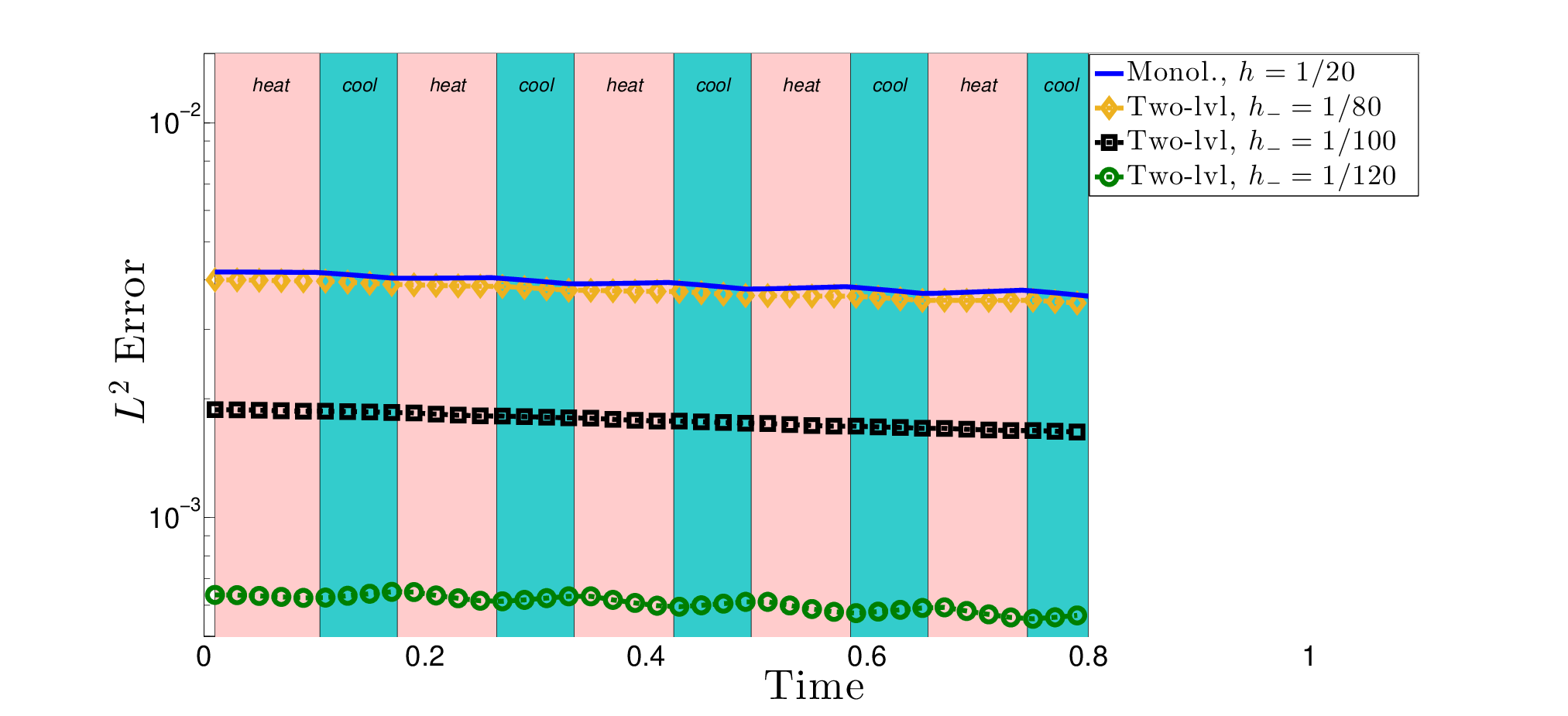
We set $T_{0}=20$ , $\beta_{+}=1.0$ , $\beta_{-}=20.0$ , $\rho_{+}=1.0$ , $\rho_{-}=5.0$ , and $\Delta t=.01$ . Our reference solution is computed on uniform fine mesh with $h=1/500$ . We then compute four solutions on a uniform global mesh with $h=1/20$ : a monolithic solution, and two-level solutions with $h_{-}=1/80,\,1/100,\,1/120$ . For all simulations, we discretize using $\mathbb{P}^{2}$ piecewise polynomial finite elements and simulate five full cycles.

We plot two relevant results. Figure 7 shows the temperature at different heights in time along the vertical line $x=.5$ , showing agreement between the two-level ( $h_{-}=1/120$ ) and reference solutions. We have colored the plot to indicate the heating and cooling phases. Figure 8 shows the relative $L^{2}$ error in time for the different solutions as compared to the reference. We observe that, although the two-level method does not give significant accuracy increases for $h_{-}=1/80$ , the performance improves noticeably as we refine $h_{-}$ . For $h_{-}=1/100$ and particularly $h_{-}=1/120$ , we significantly reduce the error when compared to the standard solution. We again emphasize that the same global mesh with $h=1/20$ was used for all simulations, and that the observed improvements result solely from refining the local mesh.

6 Conclusions

We have introduced a two-level approach for solving partial differential equations, related to the previously introduced Fat boundary method. This method is based on decomposing the problem into a split-problem formulation, then solving the two problems on different meshes in an iterative manner until convergence is achieved. It has shown particular promise for problems with prominent local characteristics, where some phenomena only occur on a (potentially small) portion of the mesh. Problems of this type occur in many areas of industrial interest, including additive manufacturing.

The proposed method contains many important and nontrivial mathematical concerns. While we have proved consistency with the original problem, a formal proof of convergence remains missing. In a similar vein, the dependance of the convergence on various parameters, including the under-relaxation parameter $\theta$ and for unsteady problems, the time step $\Delta t$ and temporal order of convergence, should be investigated. The algorithm described here also has important implications regarding the construction and application of preconditioners for the associated linear systems. We expect the outlined approach to be beneficial in this respect, as the split-problem formulation allows one to employ uniform (or quasi-uniform) meshes for the separate problems, mitigating much of the difficulty associated with preconditioning. However, this must be explored and confirmed in more detail.

For ease of presentation and mathematical analysis, we have restricted our attention in this work to cases in which $\beta_{-},\,\beta_{+},\,\rho_{-},$ and $\rho_{+}$ do not depend on the unknown $u$ . For nonlinear problems where some or all of these parameters may depend on $u$ , one must extend the approaches shown here. A natural example of such an extension is the Picard-type iterative method obtained by employing analogous two-level methods based on the splittings (2.29)-(2.32), and at an iteration $k$ , letting $\beta\left(u\right):=\beta\left(u^{k-1}\right)$ and $\rho\left(u\right):=\rho\left(u^{k-1}\right)$ . While some initial tests (not presented here) suggest this approach works, such a scheme must be analyzed and tested more rigorously. The development of a Newton-type scheme, where the nonlinear solver may converge more rapidly, is also worthy of further investigation.

From the engineering and industrial perspective, the proposed method must be further validated on more realistic problems. In particular, we intend to apply it to additive manufacturing problems of genuine engineering interest, in which we incorporate phase change and other such phenomena, in both two and three dimensions. As these problems are highly nonlinear in general, the concerns regarding the algorithm’s application to nonlinear problems is especially important.

7 Appendix: Proofs of Theorems 2.3 and 2.4

In this section, we provide proofs for Theorems 2.3 and 2.4. We note the extension of the splittings given by Problems 2.29 and 2.30 (steady) and Problems 2.31 and 2.32 (unsteady) to algorithms of the type shown in Section 3 then follow in the obvious way.

For fully nonlinear problems in which $\beta$ and/or $\rho$ are not simply non-constant but depend on the unknown temperature field $u$ , the following theorems are useful to establish the consistency of a single-step of some nonlinear iterative scheme (such as a Picard-type method). Proving the convergence of such a scheme, however, is beyond the scope of this work and an important subject for future research.

7.1 Proof of Theorem 2.3.

Proof.

Let $u$ be a solution of (2.1) where $\beta$ is understood to be non-constant. Define $\widetilde{u}$ as:

\displaystyle\widetilde{u}:=u|_{\Omega_{-}}.

(7.1)

(7.1) ensures $\widetilde{u}$ then satisfies (2.30) trivially by definition. Then for $u\in H^{1}\left(\Omega\right)$ and $\varphi\in C_{0}^{\infty}\left(\Omega\right)$ :

\displaystyle\begin{split}\int_{\Omega}\beta\nabla{u}\cdot\nabla{\varphi}&=\int_{\Omega}\beta_{+}\nabla{u}\cdot\nabla{\varphi}-\int_{\Omega_{-}}\beta_{+}\nabla u\cdot\nabla\varphi+\int_{\Omega_{-}}\beta_{-}\nabla u\cdot\nabla\varphi\\ &=\int_{\Omega}\beta_{+}\nabla{u}\cdot\nabla{\varphi}-\int_{\Omega_{-}}\beta_{+}\nabla\widetilde{u}\cdot\nabla\varphi+\int_{\Omega_{-}}\beta_{-}\nabla\widetilde{u}\cdot\nabla\varphi.\end{split}

(7.2)

We now prove a pair of brief lemmas which we will need to proceed.

Lemma 7.1.

Under the assumptions of the theorem, if $\beta_{-}\neq 0$ in $\Omega_{-}$ ,

\displaystyle-\nabla\cdot\left(\beta_{+}\nabla\widetilde{u}\right)=\frac{\beta_{+}}{\beta_{-}}f+\frac{\beta_{+}}{\beta_{-}}\nabla\widetilde{u}\cdot\nabla\beta_{-}-\nabla\widetilde{u}\cdot\nabla\beta_{+}\,\,\,\text{ in }\Omega_{-}.

(7.3)

Proof.

Since $u$ satisfies (2.1) weakly in $\Omega$ , it follows from (7.2) that

\int_{\Omega}\beta_{+}\nabla{u}\cdot\nabla{\varphi}-\int_{\Omega_{-}}\beta_{+}\nabla\widetilde{u}\cdot\nabla\varphi+\int_{\Omega_{-}}\beta_{-}\nabla\widetilde{u}\cdot\nabla\varphi=\int_{\Omega}f\varphi\,\,\,\text{ in }\Omega_{-}.

In particular, we have that:

\displaystyle-\nabla\cdot\left(\beta_{-}\nabla\widetilde{u}\right)=f\,\,\,\text{ in }\Omega_{-}.

(7.4)

We recall the product rule for the divergence of a product of a vector function $\bm{a}$ and a scalar function $b$ :

\displaystyle\nabla\cdot\left(b\bm{a}\right)

\displaystyle=b\Delta\bm{a}+\nabla b\cdot\bm{a}

(7.5)

Applying (7.5) and elementary manipulations to (7.4) gives:

\displaystyle\begin{split}-\beta_{+}\Delta\widetilde{u}&=\frac{\beta_{+}}{\beta_{-}}f+\frac{\beta_{+}}{\beta_{-}}\nabla\widetilde{u}\cdot\nabla\beta_{-}\end{split}

(7.6)

Adding and subtracting $\nabla\widetilde{u}\cdot\nabla\beta_{+}$ to (7.6), we then have:

\displaystyle\begin{split}-\beta_{+}\Delta\widetilde{u}-\nabla\widetilde{u}\cdot\nabla\beta_{+}+\nabla\widetilde{u}\cdot\nabla\beta_{+}&=\frac{\beta_{+}}{\beta_{-}}f+\frac{\beta_{+}}{\beta_{-}}\nabla\widetilde{u}\cdot\nabla\beta_{-}\\ -\nabla\cdot\left(\beta_{+}\nabla\widetilde{u}\right)&=\frac{\beta_{+}}{\beta_{-}}f+\frac{\beta_{+}}{\beta_{-}}\nabla\widetilde{u}\cdot\nabla\beta_{-}-\nabla\widetilde{u}\cdot\nabla\beta_{+}\end{split}

(7.7)

where the last line follows from applying (7.5) in reverse, completing the proof. ∎

Lemma 7.2.

Under the assumptions of the theorem, if $\beta_{-}\neq 0$ in $\Omega_{-}$ ,

\displaystyle\beta_{+}\Delta\widetilde{u}

\displaystyle=\frac{\beta_{+}}{\beta_{-}}\big[\nabla\cdot\left(\beta_{-}\nabla\widetilde{u}\right)-\nabla\beta_{-}\cdot\nabla\widetilde{u}\big]

(7.8)

Proof.

From (7.5):

\displaystyle\begin{split}\nabla\cdot\left(\beta_{+}\nabla\widetilde{u}\right)&=\nabla\beta_{+}\cdot\nabla\widetilde{u}+\beta_{+}\Delta\widetilde{u}\\ &=\nabla\beta_{+}\cdot\nabla\widetilde{u}+\frac{\beta_{+}}{\beta_{-}}\beta_{-}\Delta\widetilde{u}\\ &=\nabla\beta_{+}\cdot\nabla\widetilde{u}+\frac{\beta_{+}}{\beta_{-}}\bigg[\nabla\cdot\left(\beta_{-}\nabla\widetilde{u}\right)-\nabla\beta_{-}\cdot\nabla\widetilde{u}\bigg],\end{split}

(7.9)

where the last line follows from a second application of (7.5). This implies:

\displaystyle\begin{split}\nabla\beta_{+}\cdot\nabla\widetilde{u}+\beta_{+}\Delta\widetilde{u}&=\nabla\beta_{+}\cdot\nabla\widetilde{u}+\frac{\beta_{+}}{\beta_{-}}\bigg[\nabla\cdot\left(\beta_{-}\nabla\widetilde{u}\right)-\nabla\beta_{-}\cdot\nabla\widetilde{u}\bigg]\\ \beta_{+}\Delta\widetilde{u}&=\frac{\beta_{+}}{\beta_{-}}\bigg[\nabla\cdot\left(\beta_{-}\nabla\widetilde{u}\right)-\nabla\beta_{-}\cdot\nabla\widetilde{u}\bigg],\end{split}

(7.10)

establishing the lemma. ∎

Returning to the main theorem, integrating by parts the integrals in $\Omega_{-}$ on the right hand side of (7.2) yields:

\displaystyle\begin{split}&-\int_{\Omega_{-}}\beta_{+}\nabla\widetilde{u}\cdot\nabla\varphi+\int_{\Omega_{-}}\beta_{-}\nabla\widetilde{u}\cdot\nabla\varphi\\ \quad{}&=\int_{\Omega_{-}}\nabla\cdot\left(\beta_{+}\nabla\widetilde{u}\right)\varphi-\int_{\gamma}\beta_{+}\frac{\partial\widetilde{u}}{\partial\bm{n}}\varphi-\int_{\Omega_{-}}\nabla\cdot\left(\beta_{-}\nabla\widetilde{u}\right)\varphi+\int_{\gamma}\beta_{-}\frac{\partial\widetilde{u}}{\partial\bm{n}}\varphi\\ \end{split}

(7.11)

Which from (7.3) and (7.4) reduces to:

\displaystyle\begin{split}&-\int_{\Omega_{-}}\beta_{+}\nabla\widetilde{u}\cdot\nabla\varphi+\int_{\Omega_{-}}\beta_{-}\nabla\widetilde{u}\cdot\nabla\varphi\\ \quad{}&=\int_{\Omega_{-}}\left(1-\frac{\beta+}{\beta_{-}}\right)f\varphi-\int_{\Omega_{-}}\frac{\beta+}{\beta_{-}}\left(\nabla\widetilde{u}\cdot\nabla\beta_{-}\right)\varphi+\int_{\Omega_{-}}\left(\nabla\widetilde{u}\cdot\nabla\beta_{+}\right)\varphi+\int_{\gamma}\left(\beta_{-}-\beta_{+}\right)\frac{\partial\widetilde{u}}{\partial\bm{n}}\varphi\\ \end{split}

(7.12)

Combining (7.12) with (7.2) then gives:

\displaystyle\begin{split}&\int_{\Omega}\beta_{+}\nabla{u}\cdot\nabla{\varphi}\\ \quad{}&=\int_{\Omega_{+}}f\varphi+\int_{\Omega_{-}}\frac{\beta+}{\beta_{-}}f\varphi+\int_{\Omega_{-}}\frac{\beta+}{\beta_{-}}\left(\nabla\widetilde{u}\cdot\nabla\beta_{-}\right)\varphi\\ \quad{}&-\int_{\Omega_{-}}\left(\nabla\widetilde{u}\cdot\nabla\beta_{+}\right)\varphi+\int_{\gamma}\beta_{+}\frac{\partial\widetilde{u}}{\partial\bm{n}}\varphi-\int_{\gamma}\beta_{-}\frac{\partial\widetilde{u}}{\partial\bm{n}}\varphi,\end{split}

(7.13)

which after backward integration over $\Omega$ gives:

\displaystyle\begin{split}&-\nabla\cdot\left(\beta_{+}\nabla{u}\right)\\ \quad{}&=f\big|_{\Omega_{+}}+\frac{\beta_{+}}{\beta_{-}}f\big|_{\Omega_{-}}+\frac{\beta_{+}}{\beta_{-}}\nabla\widetilde{u}\cdot\nabla\beta_{-}\big|_{\Omega_{-}}-\nabla\widetilde{u}\cdot\nabla\beta_{+}\big|_{\Omega_{-}}+\left(\beta_{+}-\beta_{-}\right)\frac{\partial\widetilde{u}}{\partial\bm{n}}\delta_{\gamma}\text{ in }\Omega.\end{split}

(7.14)

which was to be shown.

Now let $(u,\widetilde{u})$ be a solution pair of the coupled problem. We seek to verify that $u=\widetilde{u}$ in $\Omega_{-}$ . This is equivalent to establishing that $u-\widetilde{u}$ satisfies the equation:

\displaystyle-\nabla\cdot\beta_{+}\nabla(u-\widetilde{u})=0,\quad\text{in }\Omega_{-},\qquad u-\widetilde{u}=0,\quad\text{in }\gamma,

(7.15)

which has unique solution zero. Note that $u=\widetilde{u}$ on $\gamma$ by hypothesis. For all $\varphi\in H_{0}^{1}(\Omega_{-})$ , we have⁴⁴ 4 Note that as (7.15) is zero on the boundary, we may demand this on our test space as well without loss of generality.:

$\displaystyle\int_{\Omega_{-}}\beta_{+}\nabla\left(\widetilde{u}-u\right)\cdot\nabla\varphi$	$\displaystyle=-\int_{\Omega_{-}}\nabla\cdot\left[\beta_{+}\nabla\left(\widetilde{u}-u\right)\right]\varphi$	(7.16)
	$\displaystyle=-\int_{\Omega_{-}}\nabla\cdot\left(\beta_{+}\nabla\widetilde{u}\right)\varphi+\int_{\Omega_{-}}\nabla\cdot\left(\beta_{+}\nabla u\right)\varphi$	(7.17)
$\displaystyle\begin{split}&=-\int_{\Omega_{-}}\nabla\beta_{+}\cdot\nabla\widetilde{u}\,\varphi-\int_{\Omega_{-}}\beta_{+}\Delta\widetilde{u}\,\varphi+\int_{\Omega_{-}}\nabla\cdot\left(\beta_{+}\nabla u\right)\varphi.\\ \end{split}$		(7.18)

By applying Lemma 7.2 to the middle term of (7.18), we then obtain:

\displaystyle\begin{split}&\int_{\Omega_{-}}\beta_{+}\nabla\left(\widetilde{u}-u\right)\cdot\nabla\varphi\\ &{}=-\int_{\Omega_{-}}\nabla\beta_{+}\cdot\nabla\widetilde{u}\,\varphi-\int_{\Omega_{-}}\nabla\cdot\left(\beta_{-}\nabla\widetilde{u}\right)\frac{\beta_{+}}{\beta_{-}}\varphi+\int_{\Omega_{-}}\frac{\beta_{+}}{\beta_{-}}\nabla\beta_{-}\cdot\nabla\widetilde{u}+\int_{\Omega_{-}}\nabla\cdot\left(\beta_{+}\nabla u\right)\varphi.\end{split}

(7.19)

Applying integration by parts to the second term on the right-hand side of (7.19), we observe that:

\displaystyle\begin{split}-\int_{\Omega_{-}}\nabla\cdot\left(\beta_{-}\nabla\widetilde{u}\right)\frac{\beta_{+}}{\beta_{-}}\varphi&=\int_{\Omega_{-}}\beta_{-}\nabla\widetilde{u}\cdot\nabla\left(\frac{\beta_{+}}{\beta_{-}}\varphi\right),\end{split}

(7.20)

with $\varphi\in H_{0}^{1}\left(\Omega_{-}\right)$ ensuring zero boundary terms. As $\widetilde{u}$ satisfies (2.30) weakly in $\Omega_{-}$ , this implies that for all $\varphi\in H^{1}(\Omega_{-})$ :

\displaystyle\int_{\Omega_{-}}\beta_{-}\nabla\widetilde{u}\cdot\nabla\varphi

\displaystyle=\int_{\Omega_{-}}f\,\varphi.

(7.21)

As $\beta_{+}/\beta_{-}\,\in H^{1}(\Omega_{-})$ , so too is $\frac{\beta_{+}}{\beta_{-}}\varphi\,\in H_{0}^{1}(\Omega_{-})$ and this together with (7.20) and (7.21) yields:

\displaystyle\begin{split}-\int_{\Omega_{-}}\nabla\cdot\left(\beta_{-}\nabla\widetilde{u}\right)\frac{\beta_{+}}{\beta_{-}}\varphi&=\int_{\Omega_{-}}f\,\frac{\beta_{+}}{\beta_{-}}\varphi.\end{split}

(7.22)

Substituting (7.22) into (7.19) then gives:

\displaystyle\begin{split}&\int_{\Omega_{-}}\beta_{+}\nabla\left(\widetilde{u}-u\right)\cdot\nabla\varphi\\ &{}=-\int_{\Omega_{-}}\nabla\beta_{+}\cdot\nabla\widetilde{u}\,\varphi+\int_{\Omega_{-}}f\,\frac{\beta_{+}}{\beta_{-}}\varphi+\int_{\Omega_{-}}\frac{\beta_{+}}{\beta_{-}}\nabla\beta_{-}\cdot\nabla\widetilde{u}\,\varphi+\int_{\Omega_{-}}\nabla\cdot\left(\beta_{+}\nabla u\right)\varphi.\end{split}

(7.23)

The definition of (2.29) ensures that for all $\varphi$ in $H_{0}^{1}(\Omega_{-})$ ,

\displaystyle\begin{split}-\int_{\Omega_{-}}\nabla\cdot\left(\beta_{+}\nabla u\right)\varphi&=\int_{\Omega_{-}}\frac{\beta_{+}}{\beta_{-}}f\,\varphi+\int_{\Omega}\frac{\beta_{+}}{\beta_{-}}\nabla\beta_{-}\cdot\nabla\widetilde{u}\,\varphi-\int_{\Omega_{-}}\nabla\beta_{+}\cdot\nabla\widetilde{u}\,\varphi.\end{split}

(7.24)

Substituting (7.24) into the last term on the right-hand side of (7.23) establishes:

\displaystyle\int_{\Omega_{-}}\beta_{+}\nabla\left(\widetilde{u}-u\right)\cdot\nabla\varphi

\displaystyle=0,

(7.25)

Since $u=\widetilde{u}$ in $\Omega_{-}$ , one may then easily verify that $u$ satisfies:

\displaystyle-\nabla\cdot\left(\beta\nabla u\right)

\displaystyle=f\qquad\text{in }\Omega/\penalty\gamma.

(7.26)

and that:

\displaystyle[\![\beta_{+}\nabla u\cdot\bm{n}]\!]=(\beta_{+}-\beta_{-})\frac{\partial\widetilde{u}}{\partial\bm{n}}=(\beta_{+}-\beta_{-})\frac{\partial u}{\partial\bm{n}},

(7.27)

implying that $[\![\beta\nabla\cdot\bm{n}]\!]=0$ , completing the proof. ∎

7.2 Proof of Theorem 2.4

Proof.

Let $u$ be a solution of (2.2) and define $\widetilde{u}$ as in (7.1). Then familiar arguments give: for $u\in H^{1}\left(\Omega\right)$ and $\varphi\in C_{0}^{\infty}\left(\Omega\right)$ :

\displaystyle\begin{split}&\int_{\Omega}\rho\frac{\partial u}{\partial t}\varphi+\int_{\Omega}\beta\nabla{u}\cdot\nabla{\varphi}\\ \quad{}&=\int_{\Omega}\rho_{+}\frac{\partial u}{\partial t}\varphi-\int_{\Omega_{-}}\rho_{+}\frac{\partial u}{\partial t}\varphi+\int_{\Omega_{-}}\rho_{-}\frac{\partial u}{\partial t}\varphi\\ \quad{}&+\int_{\Omega}\beta_{+}\nabla{u}\cdot\nabla{\varphi}-\int_{\Omega_{-}}\beta_{+}\nabla u\cdot\nabla\varphi+\int_{\Omega_{-}}\beta_{-}\nabla u\cdot\nabla\varphi\\ \quad{}&=\int_{\Omega}\rho_{+}\frac{\partial u}{\partial t}\varphi-\int_{\Omega_{-}}\rho_{+}\frac{\partial\widetilde{u}}{\partial t}\varphi+\int_{\Omega_{-}}\rho_{-}\frac{\partial\widetilde{u}}{\partial t}\varphi\\ \quad{}&+\int_{\Omega}\beta_{+}\nabla{u}\cdot\nabla{\varphi}-\int_{\Omega_{-}}\beta_{+}\nabla\widetilde{u}\cdot\nabla\varphi+\int_{\Omega_{-}}\beta_{-}\nabla\widetilde{u}\cdot\nabla\varphi\\ \end{split}

(7.28)

Since $u$ satisfies (2.2), from (7.28):

\displaystyle\begin{split}&\int_{\Omega}\rho_{+}\frac{\partial u}{\partial t}\varphi-\int_{\Omega_{-}}\rho_{+}\frac{\partial\widetilde{u}}{\partial t}\varphi+\int_{\Omega_{-}}\rho_{-}\frac{\partial\widetilde{u}}{\partial t}\varphi\\ \quad{}&+\int_{\Omega}\beta_{+}\nabla{u}\cdot\nabla{\varphi}-\int_{\Omega_{-}}\beta_{+}\nabla\widetilde{u}\cdot\nabla\varphi+\int_{\Omega_{-}}\beta_{-}\nabla\widetilde{u}\cdot\nabla\varphi\\ \quad{}&=\int_{\Omega}f\varphi\text{ in }\Omega,\end{split}

(7.29)

and in particular:

\displaystyle-\nabla\cdot\left(\beta_{-}\nabla\widetilde{u}\right)

\displaystyle=f-\rho_{-}\frac{\partial\widetilde{u}}{\partial t}\,\,\,\,\text{ in }\Omega_{-}.

(7.30)

After applying (7.5) to (7.31), multiply by $\beta_{+}$ and rearranging:

\displaystyle-\beta_{+}\Delta\widetilde{u}

\displaystyle=\frac{\beta_{+}}{\beta_{-}}f-\frac{\beta_{+}\rho_{-}}{\beta_{-}}\frac{\partial\widetilde{u}}{\partial t}+\frac{\beta_{+}}{\beta_{-}}\nabla\widetilde{u}\cdot\nabla\beta_{-}\,\,\,\,\text{ in }\Omega_{-}.

(7.31)

As done in (7.7), we add and subtract $\nabla\widetilde{u}\cdot\nabla\beta_{+}$ and apply (7.5), yielding:

\displaystyle-\nabla\cdot\left(\beta_{+}\nabla\widetilde{u}\right)

\displaystyle=\frac{\beta_{+}}{\beta_{-}}f-\frac{\rho_{-}\beta_{+}}{\beta_{-}}\frac{\partial\widetilde{u}}{\partial t}+\frac{\beta_{+}}{\beta_{-}}\nabla\widetilde{u}\cdot\nabla\beta_{-}-\nabla\widetilde{u}\cdot\nabla\beta_{+}\,\,\,\,\text{ in }\Omega_{-}.

(7.32)

Following the same approach as in the previous results, one integrates by parts the terms:

\displaystyle\begin{split}&-\int_{\Omega_{-}}\beta_{+}\nabla\widetilde{u}\cdot\nabla\varphi+\int_{\Omega_{-}}\beta_{-}\nabla\widetilde{u}\cdot\nabla\varphi\\ \quad{}&=\int_{\Omega_{-}}\nabla\cdot\left(\beta_{+}\nabla\widetilde{u}\right)\varphi-\int_{\gamma}\beta_{+}\frac{\partial\widetilde{u}}{\partial\bm{n}}\varphi-\int_{\Omega_{-}}\nabla\cdot\left(\beta_{-}\nabla\widetilde{u}\right)\varphi+\int_{\gamma}\beta_{-}\frac{\partial\widetilde{u}}{\partial\bm{n}}\varphi.\\ \end{split}

(7.33)

Substituting (7.31) and (7.32) into (7.33) above:

\displaystyle\begin{split}&-\int_{\Omega_{-}}\beta_{+}\nabla\widetilde{u}\cdot\nabla\varphi+\int_{\Omega_{-}}\beta_{-}\nabla\widetilde{u}\cdot\nabla\varphi\\ \quad{}&=\int_{\Omega_{-}}\left(1-\frac{\beta_{+}}{\beta_{-}}\right)f\varphi+\int_{\Omega_{-}}\left(\frac{\rho_{-}\beta_{+}}{\beta_{-}}-\rho_{-}\right)\frac{\partial\widetilde{u}}{\partial t}\\ \quad{}&-\int_{\gamma}\beta_{+}\frac{\partial\widetilde{u}}{\partial\bm{n}}\varphi+\int_{\Omega_{-}}\nabla\widetilde{u}\cdot\nabla\beta_{+}-\int_{\Omega_{-}}\frac{\beta_{+}}{\beta_{-}}\nabla\widetilde{u}\cdot\nabla\beta_{-}+\int_{\gamma}\beta_{-}\frac{\partial\widetilde{u}}{\partial\bm{n}}\varphi.\\ \end{split}

(7.34)

Combining (7.2) and (7.34):

\displaystyle\begin{split}&\int_{\Omega}\rho_{+}\frac{\partial u}{\partial t}\varphi+\int_{\Omega}\beta_{+}\nabla u\cdot\nabla\varphi\\ \quad{}&=\int_{\Omega_{-}}\left(\rho_{+}-\frac{\rho_{-}\beta_{+}}{\beta_{-}}\right)\frac{\partial\widetilde{u}}{\partial t}\varphi+\int_{\Omega_{+}}f\varphi+\int_{\Omega_{-}}\frac{\beta_{+}}{\beta_{-}}f\varphi\\ \quad{}&+\int_{\gamma}\beta_{+}\frac{\partial\widetilde{u}}{\partial\bm{n}}\varphi-\int_{\gamma}\beta_{-}\frac{\partial\widetilde{u}}{\partial\bm{n}}\varphi-\int_{\Omega_{-}}\nabla\widetilde{u}\cdot\nabla\beta_{+}+\int_{\Omega_{-}}\frac{\beta_{+}}{\beta_{-}}\nabla\widetilde{u}\cdot\nabla\beta_{-},\end{split}

(7.35)

which was to be shown.

To prove the other direction, we proceed as in the previous analyses: let $(u,\,\widetilde{u})$ solve (2.31) and (2.32) and show that $\widetilde{u}-u$ solves (2.24), after which backward integration over (7.35) gives the result.

For all $\varphi\in H_{0}^{1}(\Omega_{-}(t))$ :

\displaystyle\int_{\Omega_{-}}\rho_{+}\frac{\partial(\widetilde{u}-u)}{\partial t}\varphi-\int_{\Omega_{-}}\nabla\cdot\left[\beta_{+}\nabla(\widetilde{u}-u)\right]\varphi

\displaystyle=0

(7.36)

and hence:

\displaystyle\int_{\Omega_{-}}\rho_{+}\frac{\partial\widetilde{u}}{\partial t}\varphi-\int_{\Omega_{-}}\nabla\cdot\left(\beta_{+}\nabla\widetilde{u}\right)\varphi

\displaystyle=\int_{\Omega_{-}}\rho_{+}\frac{\partial u}{\partial t}\varphi-\int_{\Omega_{-}}\nabla\cdot\left(\beta_{+}\nabla u\right)\varphi

(7.37)

Applying (7.32) above:

\displaystyle\begin{split}&\int_{\Omega_{-}}\left(\rho_{+}-\frac{\beta_{+}\rho_{-}}{\beta_{-}}\right)\frac{\partial\widetilde{u}}{\partial t}\varphi+\int_{\Omega_{-}}\frac{\beta_{+}}{\beta_{-}}f\varphi-\int_{\Omega_{-}}\frac{\beta_{+}}{\beta_{-}}\nabla\widetilde{u}\cdot\nabla\beta_{-}\varphi+\int_{\Omega_{-}}\nabla\widetilde{u}\cdot\nabla\beta_{+}\varphi\\ {}&=\int_{\Omega_{-}}\rho_{+}\frac{\partial u}{\partial t}\varphi-\int_{\Omega_{-}}\nabla\cdot\left(\beta_{+}\nabla u\right)\varphi.\end{split}

(7.38)

From the definition of Problem (2.31), the left and right hand sides are equal, establishing $\widetilde{u}=u$ on $\Omega_{-}$ . We note that jump condition is satisfied for identical reasons as before, completing the proof. ∎

References

[1] S. Bertoluzza, M. Ismail, and B. Maury. The Fat boundary method: Semi-discrete scheme and some numerical experiments. In Domain Decomposition Methods in Science and Engineering, volume 40 of Lecture Notes in Computational Science and Engineering, pages 513–520. Springer Berlin Heidelberg, 2005.
[2] S. Bertoluzza, M. Ismail, and B. Maury. Analysis of the fully discrete fat boundary method. Numerische Mathematik, 118:49–77, 2011.
[3] C. Bruna-Russo, A. Gökhan Demir, and B. Previtali. Selective laser melting finite element modeling: Validation with high–speed imaging and lack of fusion defects prediction. Materials and Design, 156:143–153, 2018.
[4] F. Craveiro, H. Bartolo, and P. Bartolo. Functionally graded structures through building manufacturing. Advanced Materials Research, 683:775–778, 2013.
[5] K. Davey, S. Bounds, I. Rosindale, and M.T. Rasgado. A coarse preconditioner for multi-domain boundary element equations. Computers and Structures, 80(7–8):643–658, 2002.
[6] Q. Du, D. Wang, and L. Zhu. On mesh geometry and stiffness matrix conditioning for general finite element spaces. SIAM J. Numer. Anal., 47(2):1421–1444, 2009.
[7] Howard C Elman, David J Silvester, and Andrew J Wathen. Finite elements and fast iterative solvers: with applications in incompressible fluid dynamics. Oxford University Press (UK), 2014.
[8] F. Erdogan and M. Ozturk. Diffusion problems in bonded nonhomogenous materials with an interface cut. International Journal of Engineering Science, 30(10):1507–1523, 1992.
[9] X. Gao, L. Guo, and C. Zhang. Three-step multi-domain BEM solver for nonhomogenous material problems. Engineering Analysis with Boundary Elements, 31(12):965–973, 2007.
[10] D.D. Gu, W. Meiners, K. Wissenbach, and R. Poprawe. Laser additive manufacturing of metallic components: materials, processes, and mechanisms. International Materials Reviews, 57(3):133–164, 2012.
[11] Y. Huang, L.J. Yang, X.Z. Du, and Y.P. Yang. Finite element analysis of thermal behavior of metal powder during selective laser melting. International Journal of Thermal Sciences, 104:146–157, 2016.
[12] J. Irwin and P. Michaleris. A line heat input model for additive manufacturing. J. Manuf. Sci. Eng., 138(11), 2016.
[13] L. Kameski, W. Huang, and H. Xu. Conditioning of finite element equations with arbitrary anisotropic meshes. Math. Comput., 83:2187–2211, 2014.
[14] W. E. King, A. T. Anderson, R. M. Ferencz, N. E. Hodge, C. Kamath, S. A. Khairallah, and A. M. Rubenchik. Laser powder bed fusion additive manufacturing of metals; physics, computational, and materials challenges. Applied Physics Reviews, 2(4), 2015.
[15] S. Kollmannsberger, A. Ozcan, M. Carraturo, N. Zander, and E. Rank. A hierarchical computational model for moving thermal loads and phase changes with applications to selective laser melting. Computers and Mathematics with Applications, 75(5):1483–1497, 2018.
[16] N. Labonnote, A. Ronnquist, B. Manum, and P. Ruther. Additive construction: State-of-the-art, challenges and opportunities. Automation in Construction, 72(3):347–366, 2016.
[17] D.V. Le, J. White, J. Peraire, K.M. Lim, and B.C. Khoo. An implicit immersed boundary method for three-dimensinal fluid-membrane interactions. Journal of Computational Physics, 228:8427–8445, 2009.
[18] L. Lee and R.J. Leveque. An immersed interface method for incompressible Navier-Stokes equations. SIAM J. Sci. Comput., 25(3):832–856, 2003.
[19] R.J. Leveque and Z. Li. Immersed interface methods for Stokes flow with elastic boundaries or surface tension. SIAM J. Sci. Comput., 18(3):709–735, 1997.
[20] B. Maury. A Fat boundary method for the Poisson problem in a domain with holes. J. Sci. Comp., 16(3):319–339, 2001.
[21] J.R. Pacheco, A. Pacheco-Vega, T. Rodi, and R.E. Peck. Numerical simulations of heat transfer and fluid flow problems using an immersed-boundary finite-volume method on non-staggered grids. Numer. Heat Tr. B-Fund., 48:1–24, 2005.
[22] N. Patil, D. Pal, H. Khalid Rafi, K. Zeng, A. Moreland, A. Hicks, D. Beeler, and B. Stucker. A generalized feed forward dynamic adaptive mesh refinement and derefinement finite element framework for metal laser sintering–Part I: Formulation and algorithm development. Journal of Manufacturing Science and Engineering, 137(4), 2015.
[23] N. Patil, D. Pal, K.H. Kutty, K. Zeng, A. Moreland, A. Hicks, D. Beeler, and B. Stucker. A generalized feed forward dynamic adaptive mesh refinement and derefinement finite element framework for metal laser sintering–Part II: Nonlinear thermal simulations and validations. Journal of Manufacturing Science and Engineering, 138(6), 2016.
[24] D. Riedlbauer, P. Steinmann, and J. Mergheim. Thermomechanical finite element simulations of selective electron beam melting processes: Performance considerations. Comput. Mech., 54(1):109–122, 2014.
[25] M.A. Russell, A. Suoto-Iglesias, and T.I. Zohdi. Numerical simualtion of Laser Fusion Additive Manufacturing processes using the SPH method. Computer Methods in Applied Mechanics and Engineering, 341:163–187, 2018.
[26] S. Tammas-Williams and I. Todd. Design for additive manufacturing with site-specific properties in metals and alloys. Scripta Materiala, 135:105–110, 2017.
[27] Q. Wang, J. Li, M. Gouge, A.R. Nassar, P.P. Michaleris, and E.W. Reutzel. Physics-based multivariable modeling and feedback linearization control of melt-pool geometry and temperature in directed energy deposition. J. Manuf. Sci. Eng., 139(2), 2017.