YBC, a stellar bolometric corrections database with variable extinction coefficients: an application to PARSEC isochrones
Abstract
We present the YBC database of stellar bolometric corrections (BCs), available at http://stev.oapd.inaf.it/YBC. We homogenise widely-used theoretical stellar spectral libraries and provide BCs for many popular photometric systems, including the Gaia filters. The database can be easily extended to additional photometric systems and stellar spectral libraries. The web interface allows users to transform their catalogue of theoretical stellar parameters into magnitudes and colours of selected filter sets. The BC tables can be downloaded or also be implemented into large simulation projects using the interpolation code provided with the database. We compute extinction coefficients on a star-by-star basis, hence taking into account the effects of spectral type and non-linearity dependency on the total extinction. We illustrate the use of these BCs in PARSEC isochrones. We show that using spectral-type dependent extinction coefficients is quite necessary for Gaia filters whenever mag. BC tables for rotating stars and tables of limb-darkening coefficients are also provided.
Key Words.
Hertzsprung-Russell and C-M diagrams – dust, extinction – open clusters: individual: NGC 2425 – open clusters: individual: Melotte 221 Introduction
Bolometric corrections (BCs) are usually applied to the absolute magnitude of a star to obtain its bolometric absolute magnitude or luminosity, or conversely, to predict the magnitudes of a model star in a given set of filters. Most modern versions of BCs are usually based on theoretical stellar spectral libraries, e.g. Girardi et al. 2002; Casagrande & VandenBerg 2014; Casagrande & VandenBerg 2018a. In some cases empirical stellar spectral libraries are also used for this purpose, however, they require additional calibration from the theoretical atmosphere models and are always limited by the coverage of stellar spectral type and wavelength range (Sánchez-Blázquez et al. 2006; Rayner et al. 2009; Chen et al. 2014b). In practice, BCs are often provided along with, or can be easily computed from the spectral libraries obtained from the modelling of stellar atmospheres. In the present day, the widely used theoretical stellar spectral libraries include ATLAS9 (Castelli & Kurucz 2003) and PHOENIX (Allard et al. 2012) for generic types of stars, MARCS (Gustafsson et al. 2008) for cool or intermediate temperature stars, COMARCS for K/M/S/C stars (Aringer et al. 2009; Aringer et al. 2016; Aringer et al. 2019), and PoWR for Wolf-Rayet (WR) stars (Gräfener et al. 2002, and refs. therein). These libraries, with different solar abundance, offer large grids of models covering different stellar parameters (metallicity, and ). However, currently there is a lack of a single, homogeneous, public database to synthesise these libraries and provide BC tables for a large set of photometric systems.
One of the obvious advantages of having a homogeneous database for BCs would be to facilitate the comparison between stellar models and the observations. Indeed, besides the differences in the theoretical quantities such as and of various stellar models, additional deviations are often introduced from different authors using different BC tables. The possibility of testing the difference from those originally applied will become more critical with forthcoming facilities providing photometry of much higher precision: considering, for instance, the mag errors expected for Gaia sources with mag and CCD transits, for a nominal mission with perfect calibrations (Evans et al. 2018, see figure 9 in), and the systematic errors smaller than 0.005 mag planned for LSST single visits (Ivezić et al. 2019). Another aspect to consider is the different ways of handling the interstellar extinction in the models, which is especially crucial when using either UV filters (as in GALEX) or very broad passbands (such as the Gaia, TESS, and HST/WFC3/UVIS extremely wide filters). In these cases, fixed extinction coefficients are no longer valid and the effect of stellar spectral types becomes critical (Girardi et al. 2008).
In this work, we build a database where we assemble existing popular stellar spectral libraries to compute BC tables homogeneously for a wide variety of photometric systems. The web interface of this database provides a convenient way for the users to transform their theoretical stellar catalogues into magnitudes and colours, and hence to compare them with observations. It has the flexibility to choose different stellar spectral libraries, thus allowing their differences to be easily investigated. The extinction coefficients have been computed on a star-by-star basis, therefore the variation with spectral type has been taken into account. The non-linearity as a function of has been included, which is important for highly attenuated targets.
In this paper, we introduce the definitions of the BCs in section 2, the available stellar spectral libraries in section 3 and our C/Python code package in section 4. We compare some of our results with the literature in section 5. In section 6, we discuss the spectral type dependent extinction coefficients. Section 7 summarises the main results.
2 Bolometric corrections
In this section, we recall some basic relations concerning the bolometric correction which are necessary for the discussion. We refer the readers to Kurucz 1979, Bessell et al. 1998, and Girardi et al. 2002 for a more exhaustive discussion.
First, we recall the definition of magnitude. Assuming we (at earth) receive a radiation flux (or ) from a source, the magnitude in a certain filter band with transmission curve is
| (1) |
In this equation, is the flux of the reference spectrum and is the corresponding reference magnitude. These two quantities depend on the photometric system and will be discussed later. and denote the lower and upper wavelength limits of the filter transmission curve, respectively. The above equation is valid for present-day photon-counting devices (CCDs or IR arrays). For more traditional energy-integrating systems the above equation should be changed to
| (2) |
Depending on the reference spectra (or ), commonly used magnitude systems are:
- •
Vega magnitude systems. The spectrum of Vega ( Lyr) is used as the reference spectrum. The reference magnitudes are set so that Vega has a magnitude equal to, or slightly different from zero. By default, we use the latest Vega spectrum11 1 Currently it is alpha_lyr_stis_008.fits from ftp://ftp.stsci.edu/cdbs/current_calspec/. from the CALSPEC database (Bohlin et al. 2014).
- •
AB magnitude systems (Oke 1974). The reference spectrum has a constant value of . The reference magnitudes thus are set to 48.60 mag.
- •
Space Telescope (ST) magnitude systems (Laidler V. et al. 2005). The reference spectrum has a constant value of . The reference magnitudes thus are set to 21.10 mag.
- •
Gunn systems (Thuan & Gunn 1976). In these systems, F-type subdwarfs, in particular BD +17 4708, are taken as the reference stars instead of Vega.
Among these, the Vega and AB magnitude systems are the most widely adopted ones. At http://stev.oapd.inaf.it/cmd/photsys.html, the reader can check the information about the photometric systems supported.
Usually, synthetic spectral libraries provide the stellar flux at the stellar radius . This flux is related to the effective temperature of the star by
| (3) |
where is the Stefan-Boltzmann constant. By placing the star at 10 pc from the earth, the flux we receive is
where is the assumed extinction between the star and the observer. Therefore, the absolute magnitude for a photon-counting photometric system is
| (4) |
The definition of bolometric magnitude is
| (5) |
According to the IAU 2015 resolution (Mamajek et al. 2015), the absolute bolometric magnitude for the nominal solar luminosity ( W) is mag.
Given an absolute magnitude in a given filter band for a star of absolute bolometric magnitude , the bolometric correction is:
| (6) |
By combing equations (4), (5) and (6), we have
| (7) |
The advantage of using the above equation to compute BCs is that the stellar radius disappears. In some cases, the stellar spectral library is computed in plane-parallel geometry and there is no definition of a geometrical stellar radius (but the optical depth). Therefore, once (related to by equation (3)) for a star with given , and metallicity is provided, the corresponding can be derived.
The above definition of the BC is valid for present-day photon-counting devices (CCDs or IR arrays), while for energy-integrating systems the above equation should be changed to
| (8) |
For AB magnitude systems with photon-counting devices, we can either convert to and use equation (7), or use the following equation instead:
| (9) |
Similarly, the equation for AB magnitude system with energy-integrating devices is:
| (10) |
3 Stellar spectral libraries
In this section, we briefly describe the stellar spectral libraries currently supported in our database. We will continuously expand it with data from external sources or provided by our group.
3.1 ATLAS9 models
One of the most widely used stellar spectral libraries is the plane parallel models computed by Castelli & Kurucz 200322 2 http://wwwuser.oats.inaf.it/castelli/grids.html. with the ATLAS9 code (Kurucz 2014). These models are based on the solar abundances by Grevesse & Sauval 1998 and make use of an improved set of molecular absorption lines including TiO and , as well as absorption lines from quasi-molecular H-H and H-H+. The model grids are computed for from 3500 K to 50000 K, ( in cgs unit) from 0.0 dex to 5.0 dex and [M/H]=+0.5, +0.2, 0.0, 0.5, 1.0, 1.5, 2.0, 2.5, 3.5, 4 and 5.5.
3.2 PHOENIX models
The PHOENIX database (Allard & Hauschildt 1995; Allard et al. 1997) is another widely used stellar spectra library, especially for cool stars. The atmospheres of cool stars are dominated by molecular formation and by dust condensation at very low temperature. Both of these two phenomena can affect the spectral shape significantly. A suitable set of 1D, static spherical atmosphere spectral models accounting for the above effects has been provided in Allard et al. 2012. Among the different model suites of this database, we use the BT-Settl33 3 https://phoenix.ens-lyon.fr/Grids/BT-Settl/AGSS2009/. models for the coverage completeness in stellar parameters and for the wide usage in the literature. The BT-Settl models use the Asplund et al. 2009 solar abundances. They are provided for K , , and metallicities .
3.3 WM-basic models
For temperatures typical of O and B stars (19000 K60000 K) we have computed a library of models using the public code WM-basic (Pauldrach et al. 1986), as described in Chen et al. 2015. This allows us to consider both the effects of extended winds and those of non-LTE, because both effects may significantly affect the emergent spectra of hot stars. These models use the solar abundances of PARSEC (Bressan et al. 2012), which compiled the results from Grevesse & Sauval 1998, Caffau et al. 2011 and references therein. The model grids are computed for metallicities of , 0.0005, 0.001, 0.004, 0.008 and 0.02. covers the interval from 4.3 to 5 with a step of 0.025 dex, while goes from 2.5 to 6.0 with a step of 0.5 dex. For each and , models with three values of mass loss rate (, , and ) are computed if convergence is reached for them, as detailed in Chen et al. 2015.
3.4 PoWR models
Wolf-Rayet (WR) stars typically have wind densities one order of magnitude larger than those of massive O-type stars. Spectroscopically they are dominated by the presence of strong broad emission lines of helium, nitrogen, carbon and oxygen. They are subdivided into different sub-types, one with strong lines of helium and nitrogen (WN stars), another one with strong lines of helium and carbon (WC stars) and the third one with strong oxygen lines (WO stars). The PoWR44 4 http://www.astro.physik.uni-potsdam.de/~wrh/PoWR/powrgrid1.php. group has provided models for WR stars (Gräfener et al. 2002; Hamann & Gräfener 2004; Sander et al. 2012; Todt et al. 2015). These models adopt the solar abundances from Grevesse & Sauval 1998, and are computed for Milky Way, Large Magellanic Cloud (LMC), Small Magellanic Cloud (SMC), and sub-SMC metallicities. For each metallicity, late-type WN stars of different hydrogen fraction, early-type WN stars, and WC (except for SMC and sub-SMC at the moment) stars are computed. For a given spectral type and metallicity, the models are computed as a function of and the transformed radius (Schmutz et al. 1989) (which is a more important quantity than in these models dominated by stellar winds). The coverage in () and () changes with metallicity and spectral type. The transformed radius is defined as:
| (11) |
with , and being the hydro-static stellar radius, terminal velocity and mass loss rate, respectively. Notice that in the original definition of of PoWR, a multiplication factor is applied to the above equation, where is the clumping factor. For different types of WR models of PoWR, different clumping factors have been used. To facilitate the interpolation, we have divided the values from PoWR by this factor, therefore it disappears in the above equation.
3.5 COMARCS models
The local thermodynamic equilibrium (LTE) & chemical equilibrium without dust, spherical symmetric, hydrostatic COMARCS55 5 http://stev.oapd.inaf.it/atm.,66 6 http://stev.oapd.inaf.it/synphot/Cstars. database provides models for C, S, K and M type stars for modelling TP-AGB stars and other red giants (Aringer et al. 2009; Aringer et al. 2016; Aringer et al. 2019). The solar chemical composition is based on Caffau et al. 2009a; Caffau et al. 2009b. The carbon star grids cover a metallicity Z range from 0.001 to 0.016, from 2500 K to 4000 K and from 1 to 2, while the K/M star grids cover a metallicity range from 0.00016 to 0.14, from 2600 K to 4800 K and from 1 to 5.
3.6 DA white dwarf spectral libraries
Gaia DR2 parallaxes (Luri et al. 2018) allowed to place a quite significant number of white dwarfs into absolute magnitude versus colour diagrams, hence ensuring a wide interest in including these objects in isochrone-fitting methods. Therefore we include the Koester 2010 and Tremblay & Bergeron 2009 DA white dwarf libraries (downloaded from http://svo2.cab.inta-csic.es/theory/newov/) in our database. In these plane-parallel models LTE and hydro-static equilibrium are assumed. The library covers the range from 5000 K to 80000 K, ranges from 6.5 to 9.5.
3.7 ATLAS12 models with -enhancement
For studying the photometric properties of alpha-enhanced PARSEC stellar models, we have computed atmosphere models with the latest ATLAS12 code77 7 https://www.oact.inaf.it/castelli/castelli/sources/atlas12.html. with an updated line lists. These models have been used in Fu et al. 2018, and have been shown to improve the fitting to the Galactic Globular Cluster 47Tuc observations with HST ACS/WFC3. For the moment, we only computed these spectra for two metallicities corresponding to two 47 Tuc stellar populations (Fu et al. 2018), however, work is in progress to extend them to other metallicities together with the PARSEC alpha-enhanced stellar tracks. These models cover from 4000 K to 21000 K, and from 0.5 to 5. Below 10000 K, the step in is 100 K, while above the step is 200 K. The step in is 0.5 dex.
3.8 Spectra of rotating stars based on Kurucz models
In Girardi et al. 2019, we have computed a spectral library for rotating stars with a new approach. This approach takes into account the effect of the stellar surface effective temperature variation due to rotation – which results in the photometric differences when the star is observed from different angles – as well as the limb-darkening effect. This library is based on the spectral intensity library from Kurucz http://www.kurucz.havard.edu. The Kurucz models cover from 3500 K to 50000 K, from 0 to 5, and [M/H] from 5 to +1. The wavelength coverage is the same as that of ATLAS9 models, from 90.9 Å to 16 m.
3.9 Tables of limb-darkening coefficients
The limb-darkening effect is important to analyse light curves of eclipsing binaries and microlensing events, and for probing exoplanet atmospheres and spatially resolved stellar surfaces. Accurate empirical determination of limb-darkening coefficients through eclipsing binaries observations is not possible yet, mainly because of parameter degeneracies. Therefore, stellar atmosphere models are essential in these studies. Based on the spectral intensity library from the Kurucz website (http://www.kurucz.havard.edu), we computed the specific intensity as a function of , where is the angle between the line of sight and the surface normal, for each of the filter systems we have. Specific intensities have been computed for both photon-counting and energy-integrating detectors respectively as
| (12) |
and
| (13) |
We further computed the limb-darkening coefficients (, , and ) with the fitting relation proposed by Claret 2000:
| (14) |
These coefficients are provided mainly for a question of completeness. Indeed, they are computed homogeneously for all filter sets included in our database.


3.10 Stellar spectral library selection
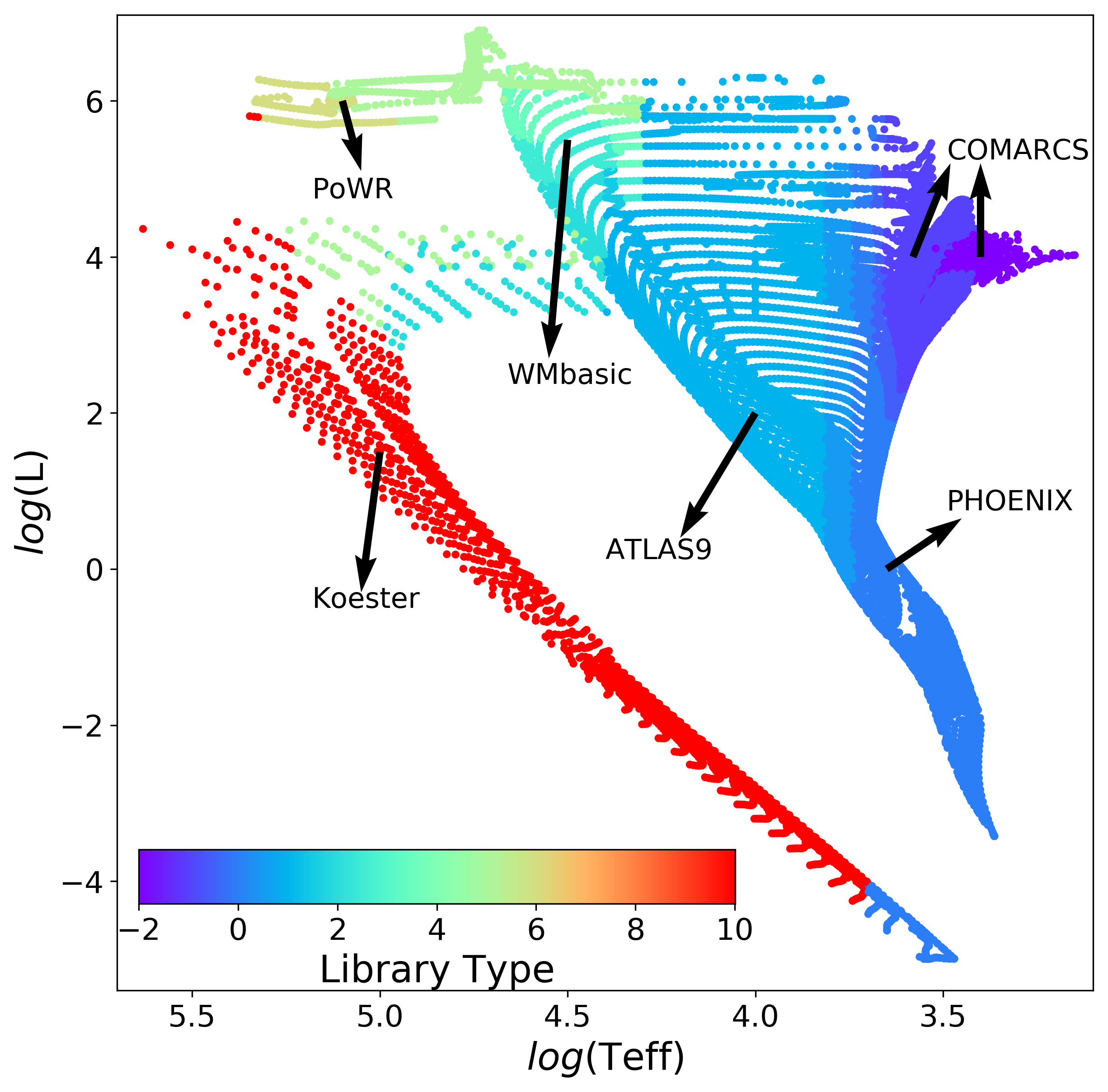
The above-described libraries can be used either combined or separately. The default library selection scheme is:
- 1)
ATLAS9 is used when K;
- 2)
PHOENIX is used when K;
- 3)
a smooth interpolation between the previous two when K;
- 4)
COMARCS M/S star library is used when and K and ;
- 5)
a smooth interpolation between PHOENIX and COMARCS M/S star library in the overlapping region between them;
- 6)
COMARCS C star library is used when and K and ;
- 7)
WM-basic libraries are used when K and the mass loss rate ;
- 8)
PoWR libraries are used when K or or , where represents the original surface hydrogen mass fraction;
- 9)
when PoWR libraries are selected and and , PoWR WC library is used;
- 10)
Koester WD library is used when and K.
The stellar surface chemical compositions are used in the above scheme, therefore they are required in the web interface (see Appendix A for more details). If the required chemical abundances are not provided by the user, a solar scaled abundance is used with the specified metallicity , which means all the relevant abundance ratios are the same as those in the Sun. As a test case we have applied the new bolometric corrections to the PARSEC V1.2s isochrones. In Figure 1, we show the isochrones with [M/H]=0 and for selected ages, in the standardised system from Bessell 1990, and in the Gaia DR2 passband as described in Maíz Apellániz & Weiler 2018 (the Gaia filters used in the following sections are also from this reference, unless specified otherwise). Different colours indicate the different stellar spectral libraries adopted, as specified in the caption.
Beside the above default scheme, we also offer some other options, such as ATLAS9 only, PHOENIX only, or a combination of them (with an adjustable transition region), etc. An issue concerns the difference in broad band CMDs between different libraries. We take the comparison between ATLAS9 and PHOENIX as an example to address this issue. In Figure 2 we show the differences between PHOENIX and ATLAS9 libraries in several CMDs, using the same PARSEC v1.2S isochrones of [M/H]=0.0 and ages log(age/yr)=8, 9 and 10. The difference between PHOENIX and ATLAS9 increases at decreasing . At the solar metallicity, the colour difference between these two atmosphere models can reach mag at the main sequence turn-off and mag at the giant branch in the V-(V-I) plane. For the lower main sequence stars, we have shown in our previous work (Chen et al. 2014a) that PHEONIX offers a better fitting compared to ATLAS9. Moreover, the PHOENIX library is computed with spherical geometry, making it preferable than ATLAS9 models especially for giants.
4 The code package and web interface
The design of this package is to make it transparent to the user, extensible to adopting new stellar spectral libraries, filter sets, and definitions of photometric systems.
The whole package is divided into three parts/steps. In the first step, the original stellar spectral libraries are assembled and re-sampled to FITS/HDF5 format files. In the second step, these files are used to compute bolometric corrections. In the third step, these BC tables are used in interpolation for stars of given stellar parameters. The code for the first and second steps is written in Python because the computational speed is not an issue and we only need to compute those tables once for all. Compared to C or Fortran, Python provides high-level libraries for manipulating tabular data (including ASCII, FITS and HDF5 formats). The third step is written in C language for a faster computational speed.
4.1 Assembled FITS/HDF5 files of spectra
In this step, the original spectra are assembled into FITS (Wells et al. 1981) and/or HDF5 (Koziol & Robinson 2018) format files. If the original spectra are in very high resolution, eg. the PHOENIX models contain wavelength points which are not necessary for the BC calculation except for narrow band filters, they are re-sampled into a lower resolution wavelength grid before assembling for computational speed and file size. The re-sampling is done with a modified version of SpectRes package (Carnall 2017), which preserves the integrated flux within each of the wavelength grids. After this step, the stellar spectral libraries are store in homogeneous file format and organisation. This step is necessary as the original stellar spectral libraries are provided in different formats. For example, the PHOENIX models are stored in a single ASCII file for each spectrum, while ATLAS9 models are stored in one single ASCII file for all the models of a given metallicity. Currently, the assembled spectra for non-rotating stars are stored in FITS format and can be easily viewed with TOPCAT (Taylor 2017), while the assembled spectra for rotating stars are stored in HDF5 format for their logically complexity.
4.2 Computing tables of BCs
In this step, the above-generated FITS format spectra are read to compute the BCs, for different filter sets available, according to equations (7) to (10). The BCs are first computed for the original grids. However, these original grids are usually not rectangular or uniformly distributed in the – () plane. For example, at high , usually the high models are missing due to the proximity to the Eddington limit. We always extend the grids in with neighbouring models of the same . Thereafter, these rectangular grids are re-sampled in – () plane with fixed steps. This re-sampling enables fast index searching for the interpolation when utilising the BC tables. These final BC tables are stored into FITS format files. BCs with different s are assembled in to the same file, therefore the reader can easily check some of the discussions presented in section 6 (such as Figure 4). Furthermore, this Python package provides an option to use “gnu-parallel” tool (Tange 2011) for computing tables for many different filter sets in parallel.
4.3 Interpolation scheme
After the BC tables are computed, users can use these tables with their own interpolation code, or a C code provided by us upon request. In summary, this code employs linear interpolations in , or , and . First, the BC tables in a specified filter set are loaded into the memory. An input star is then assigned a label according to its and (or for WRs), or also spectral type in the case of WRs. This label tells the code which libraries are assigned. If this star is in the transition region between two libraries, both libraries are selected. A weight is given according to the proximity of the star to each library. Within a library, the interpolation is done in the and grids of two neighbouring metallicities and then between the two metallicities. Because the and grids are pre-sampled at fixed grids, the interpolation in the and plane is very fast. For instance, with a computer of 3.6 GHz CPU, it takes less than 20 seconds for a catalogue of stars in the standard filters. The memory consumption is less than 20 Mby.
In the interpolation, there are issues concerning the metallicities used in different stellar spectral libraries. Different libraries were computed with different solar abundances and different -enhancement. Part of the difference presented in the figure 2 comes from the metallicity difference. Moreover, the isochrones or theoretical stars may have solar abundances and -enhancement different from the stellar atmosphere models. Currently, we only consider the total metallicities () for each of the libraries. The total metallicities are computed with their own solar abundances. Though different solar abundances and -enhancements affect the detailed spectral features, the broad-band BCs are less affected and the interpolation in the total metallicities can be taken as the first-order approximation. We have recorded the solar abundances and -enhancements information in the code and may consider these effects when a better interpolation scheme is defined. We are also computing atmosphere models with the same abundances as used for computing PARSEC tracks, with the ATLAS12 code. These models will ensure the consistency between the atmosphere models and PARSEC stellar models, and may also allow us the evaluate the above issues.
4.4 Web interface
We build an easy-to-use web interface (http://stev.oapd.inaf.it/YBC) for the users to directly convert any uploaded catalogue containing theoretical quantities into magnitudes and colours (not necessarily the PARSEC ones). More details about the web interface are provided in appendix A.
The above assembled spectral libraries, as well as the BC tables in different filters, can be downloaded at the “Spectral libraries” and the “BC tables” sections of this website, respectively.
5 Comparison with literature results
In this section, we compare our BCs derived from ATLAS9 models with those from some well-known studies on the temperature scales or bolometric corrections. It is intended mainly as a general consistency check, rather than a detailed comparison.
Ramírez & Meléndez 2005 provide empirical temperature scales for stars with K and . In the upper panels of Figure 3, we compare their and vs. relations with ours. They are consistent to within mag. We also plot the empirical relations for the dwarfs/sub-giants from Casagrande et al. 2010, which improve the comparison with the theoretical ones for the relatively hot stars, but behave oppositely for cooler stars. This may indicate that there are still some large uncertainties in determining the physical parameters for cool stars. Casagrande & VandenBerg 2014; Casagrande & VandenBerg 2018a; Casagrande & VandenBerg 2018b presented a code to compute the BCs based on the MARCS (Gustafsson et al. 2008) atmosphere models. In the middle panels of Figure 3, we show the comparison for both the and colours. We find a very good agreement between ours and theirs. Finally, in the bottom panels we compare our BCs with those based on 3D atmosphere models from Chiavassa et al. 2018. The agreement is also quite reasonable, except from some departure at low . This might implicate that the atmospheres of cool stars could be better modelled with 3D models.
The above comparisons indicate that there is a general agreement between theoretical BCs derived from different 1D models or 3D models (except for cool stars), while there is some non-negligible difference between 1D models and empirical relations or 3D ones, especially for cool stars, which deserves further investigation to solve the discrepancies.


6 Spectral type dependent extinction coefficients
Interstellar extinction is included into equations (7) and (8) using extinction curves computed with the ‘‘extinction’’88 8 https://extinction.readthedocs.io. Python routine, which includes most of the popular extinction laws in the literature. By default, our database is computed using Cardelli et al. 1989 plus O’Donnell 1994 extinction law (CCM+O94) with , to keep consistency with the CMD web-page. However, other extinction laws with different can be computed upon request. For example, we also include the extinction curve from Wang & Chen 2019 (private communication), in which they found a non-negligible discrepancy with that of Cardelli et al. 1989 along our Galaxy by using a large data-set of photometry from Gaia DR2 and other surveys. In the following discussion, if not specified, CCM+O94 is used.
The effect of extinction on each passband can be easily evaluated by looking at the quantity . For very narrow filters or for hypothetical monochromatic sources, the relationship between and would be linear. However, in the general case of a broad filter, where the stellar flux can change significantly within the filter wavelength range, the quantity will vary both as a function of spectral type, and as a function of the total . This can be seen in Figure 4, where we plot as a function of (=1, 2, and 3 mag) for the Gaia band (Maíz Apellániz & Weiler 2018), the Gaia colour and the WFC3/UVIS F218W magnitude (also see Girardi et al. 2008, for ACS filters), using the ATLAS9 spectral library. The grey open circles denote the models with fixed extinction coefficients at the filter centres, which are connected by the solid lines. At every the dispersion is caused by different and to a lesser extent also by (which cannot be seen in this figure, but is clear when checking the BC tables). At mag, there is already a mag difference in the Gaia band, mag in the Gaia colour, and mag in the F218W filter. Therefore, we suggest to use spectral-type dependent extinction coefficients for Gaia filters and UV filters whenever mag. This dispersion increases significantly with increasing . At mag, for instance, the dispersion is about 1 magnitude for the Gaia band. This means that spectral type dependent extinction coefficients are quite necessary, especially at large . Qualitatively speaking, fixed extinction coefficients would make hot stars bluer and cool stars redder compared to the case with variable extinction coefficients.
Furthermore, for a given spectrum and filter band, is not a linear function of . Figure 4 shows that at the effect brought by the non-linearity is mag in the Gaia colour for a solar type model. Therefore, a constant extinction coefficient (which could be derived by only computing the BCs with and mag) for all s is not applicable. To properly consider the effect of extinction, we compute the BC tables with [0, 0.5, 1, 2, 5, 10, 20] mag for each of the spectra in our database. These tables will be used for interpolation in , to derive BCs for any intermediate value of .
Here we show an example of isochrone fitting for NGC 2425 with Gaia DR2 data. The cluster is chosen because of its relatively large extinction and relatively old age. For this open cluster, Bossini et al. 2019 presented isochrone fitting parameters of mag, a true distance modulus DM0=12.644 mag, age=2.15 Gyr and dex. Our intention here is just to demonstrate the effect of variable extinction coefficients, rather than obtaining a perfect isochrone fitting. Therefore, we fix dex and the true distance modulus (12.644 mag) as in Bossini et al. 2019, and vary only the way the extinction is applied to isochrones, and their ages. The best-fitting isochrones with variable extinction coefficients based on Fitzpatrick & Massa 2007 and CCM+O94 extinction laws are plotted with red solid and blue dashed lines. The isochrone with FM07 extinction law has an 0.23 Gyr older age and 0.1 mag smaller extinction than that with CCM+O94 extinction law. The best-fitting isochrones with fixed extinction coefficients based on FM07 extinction law is plotted as the green dot-dashed line. It has an 0.16 Gyr older age and 0.25 mag smaller extinction. These numbers represent the uncertainties in isochrone fitting for an object with mag, when different extinction approaches are used. We also notice that our best fitting isochrone with FM07 extinction law predicts Gyr older age but similar extinction than that of Bossini et al. 2019, though we used the same PARSEC model set, atmosphere models. The extinction coefficients used in Bossini et al. 2019 (which is from Gaia Collaboration et al. 2018) are derived with FM07 extinction law. We plot the same isochrone as the red solid line but with the extinction coefficients from Bossini et al. 2019, which is shown as the black dotted line. They are quite similar, thus the large difference in age should be due to other sources. However, this is out of the scope of this work.


To further investigate the effect of using different extinction law, we plot the BC differences with FM07, CCM+O94 and that of Bossini et al. 2019 in Figure 6. In the range of , which comprises most of the NGC 2425 data, the colour difference between FM07 and CCM+O94 cases is about 0.41 mag, and it explains most of the differences in the derived physical parameters for isochrone fitting. the colour difference between FM07 and that of Bossini et al. 2019 cases is about 0.15 mag, to which some numerical errors might have contributed. Furthermore, at lower , there is a quite large dispersion in the BCs due to the variations in . We thus find that, for the stellar atmospheres adopted here, the effect of using different extinction law and the gravity dependency at low temperatures is not small and should be included in extinction parameterisation.
The above discussions imply that to derive the stellar/cluster age and extinction more accurately, BCs that take into account the spectral type are urgently needed, especially for objects with large extinction.
7 Summary and Conclusions
In this paper, we present a homogeneous database of bolometric corrections (YBC) for a large number of popular photometry systems, based on a variety of stellar spectral libraries we collected from the public domains, or computed in our previous works. In this database, the BC tables both without extinction and with extinctions until are computed. Therefore, our YBC database provides a more realistic way to fit isochrones with a spectral type dependent extinction, and allow users to choose the atmosphere models that best for their science needs. The YBC database and software package are incorporated into the PARSEC isochrones provided via the web interface CMD99 9 http://stev.oapd.inaf.it/cgi-bin/cmd..
A potential application of this database is to incorporate it into large simulation programs, with the interpolation routine provided. For example, we have implemented this database in to TRILEGAL for stellar population simulations (Girardi et al. 2005; Girardi 2016).
Our database can be also quite useful for stellar evolution model comparison. For example, people studying star clusters may fit stellar evolution models from different groups to the observation data. However, different groups may provide photometric magnitudes with BCs from different libraries. Through our package, they can convert theoretical quantities into photometric magnitudes of the same libraries.
Finally, we also show an example of the isochrone fitting to a younger cluster, Melotte 22, with the Gaia DR2 data in Fig. 7. It presents a quite well sampled main-sequence, spanning almost 3.5 magnitudes in colour. It can be seen that isochrones adopting the present BC tables describe very well the entire sequence, except perhaps for the reddest and faintest stars, which can be affected by larger photometric errors, as well as by uncertainties in pre-MS models and in their surface boundary conditions (Chen et al. 2015, see).
Work is ongoing to compute -enhanced evolutionary models with and without rotation with the PARSEC code. Meanwhile, we are also computing -enhanced stellar atmosphere models with ATLAS12 code, to extend the present database with -enhanced stellar spectral libraries. These spectral libraries will be incorporated in the web interface. We will also implement the MARCS atmosphere models (Gustafsson et al. 2008) into our database. BCs derived from 3D atmosphere models will also be included in the future.
Acknowledgements
We acknowledge the support from the ERC Consolidator Grant funding scheme (project STARKEY, G.A. n. 615604). We thank Dr. Angela Bragaglia and Dr. Diego Bossini for useful discussions on clusters. We thank Dr. Bengt Edvardsson for the help on MARCS atmosphere models. We thank Dr. Xiaodian Chen for kindly providing us the Python routine computing their extinction law. This research made use of Astropy,1010 10 http://www.astropy.org. a community-developed core Python package for Astronomy (Astropy Collaboration et al. 2013; Price-Whelan et al. 2018). We are grateful to the referee for useful suggestions.
References
- Allard & Hauschildt (1995) Allard, F. & Hauschildt, P. H. 1995, ApJ, 445, 433
- Allard et al. (1997) Allard, F., Hauschildt, P. H., Alexander, D. R., & Starrfield, S. 1997, ARA&A, 35, 137
- Allard et al. (2012) Allard, F., Homeier, D., Freytag, B., & Sharp, C. M. 2012, in EAS Publications Series, Vol. 57, EAS Publications Series, ed. C. Reylé, C. Charbonnel, & M. Schultheis, 3–43
- Aringer et al. (2016) Aringer, B., Girardi, L., Nowotny, W., Marigo, P., & Bressan, A. 2016, MNRAS, 457, 3611
- Aringer et al. (2009) Aringer, B., Girardi, L., Nowotny, W., Marigo, P., & Lederer, M. T. 2009, A&A, 503, 913
- Aringer et al. (2019) Aringer, B., Marigo, P., Nowotny, W., et al. 2019, MNRAS, 487, 2133
- Asplund et al. (2009) Asplund, M., Grevesse, N., Sauval, A. J., & Scott, P. 2009, ARA&A, 47, 481
- Astropy Collaboration et al. (2013) Astropy Collaboration, Robitaille, T. P., Tollerud, E. J., et al. 2013, A&A, 558, A33
- Bessell (1990) Bessell, M. S. 1990, PASP, 102, 1181
- Bessell & Brett (1988) Bessell, M. S. & Brett, J. M. 1988, PASP, 100, 1134
- Bessell et al. (1998) Bessell, M. S., Castelli, F., & Plez, B. 1998, A&A, 333, 231
- Bohlin et al. (2014) Bohlin, R. C., Gordon, K. D., & Tremblay, P.-E. 2014, PASP, 126, 711
- Bossini et al. (2019) Bossini, D., Vallenari, A., Bragaglia, A., et al. 2019, A&A, 623, A108
- Bressan et al. (2012) Bressan, A., Marigo, P., Girardi, L., et al. 2012, MNRAS, 427, 127
- Caffau et al. (2009a) Caffau, E., Ludwig, H. G., & Steffen, M. 2009a, Mem. Soc. Astron. Italiana, 80, 643
- Caffau et al. (2011) Caffau, E., Ludwig, H. G., Steffen, M., Freytag, B., & Bonifacio, P. 2011, Sol. Phys., 268, 255
- Caffau et al. (2009b) Caffau, E., Maiorca, E., Bonifacio, P., et al. 2009b, A&A, 498, 877
- Cardelli et al. (1989) Cardelli, J. A., Clayton, G. C., & Mathis, J. S. 1989, ApJ, 345, 245
- Carnall (2017) Carnall, A. C. 2017, arXiv e-prints, arXiv:1705.05165
- Casagrande et al. (2010) Casagrande, L., Ramírez, I., Meléndez, J., Bessell, M., & Asplund, M. 2010, A&A, 512, A54
- Casagrande & VandenBerg (2014) Casagrande, L. & VandenBerg, D. A. 2014, MNRAS, 444, 392
- Casagrande & VandenBerg (2018a) Casagrande, L. & VandenBerg, D. A. 2018a, MNRAS, 475, 5023
- Casagrande & VandenBerg (2018b) Casagrande, L. & VandenBerg, D. A. 2018b, MNRAS, 479, L102
- Castelli & Kurucz (2003) Castelli, F. & Kurucz, R. L. 2003, in IAU Symposium, Vol. 210, Modelling of Stellar Atmospheres, ed. N. Piskunov, W. W. Weiss, & D. F. Gray, A20
- Chen et al. (2015) Chen, Y., Bressan, A., Girardi, L., et al. 2015, MNRAS, 452, 1068
- Chen et al. (2014a) Chen, Y., Girardi, L., Bressan, A., et al. 2014a, MNRAS, 444, 2525
- Chen et al. (2014b) Chen, Y.-P., Trager, S. C., Peletier, R. F., et al. 2014b, A&A, 565, A117
- Chiavassa et al. (2018) Chiavassa, A., Casagrande, L., Collet, R., et al. 2018, A&A, 611, A11
- Claret (2000) Claret, A. 2000, A&A, 363, 1081
- Cohen et al. (2003) Cohen, M., Wheaton, W. A., & Megeath, S. T. 2003, AJ, 126, 1090
- Evans et al. (2018) Evans, D. W., Riello, M., De Angeli, F., et al. 2018, A&A, 616, A4
- Fitzpatrick & Massa (2007) Fitzpatrick, E. L. & Massa, D. 2007, ApJ, 663, 320
- Fu et al. (2018) Fu, X., Bressan, A., Marigo, P., et al. 2018, MNRAS, 476, 496
- Gaia Collaboration et al. (2018) Gaia Collaboration, Babusiaux, C., van Leeuwen, F., et al. 2018, A&A, 616, A10
- Girardi (2016) Girardi, L. 2016, Astronomische Nachrichten, 337, 871
- Girardi et al. (2002) Girardi, L., Bertelli, G., Bressan, A., et al. 2002, A&A, 391, 195
- Girardi et al. (2019) Girardi, L., Costa, G., Chen, Y., et al. 2019, MNRAS, 488, 696
- Girardi et al. (2008) Girardi, L., Dalcanton, J., Williams, B., et al. 2008, PASP, 120, 583
- Girardi et al. (2005) Girardi, L., Groenewegen, M. A. T., Hatziminaoglou, E., & da Costa, L. 2005, Astronomy and Astrophysics, 436, 895
- Gräfener et al. (2002) Gräfener, G., Koesterke, L., & Hamann, W.-R. 2002, A&A, 387, 244
- Grevesse & Sauval (1998) Grevesse, N. & Sauval, A. J. 1998, Space Sci. Rev., 85, 161
- Gustafsson et al. (2008) Gustafsson, B., Edvardsson, B., Eriksson, K., et al. 2008, A&A, 486, 951
- Hamann & Gräfener (2004) Hamann, W.-R. & Gräfener, G. 2004, A&A, 427, 697
- Ivezić et al. (2019) Ivezić, Ž., Kahn, S. M., Tyson, J. A., et al. 2019, ApJ, 873, 111
- Jordi et al. (2010) Jordi, C., Gebran, M., Carrasco, J. M., et al. 2010, A&A, 523, A48
- Koester (2010) Koester, D. 2010, Mem. Soc. Astron. Italiana, 81, 921
- Koziol & Robinson (2018) Koziol, Q. & Robinson, D. 2018, HDF5, [Computer Software] https://doi.org/10.11578/dc.20180330.1
- Kurucz (1979) Kurucz, R. L. 1979, ApJS, 40, 1
- Kurucz (2014) Kurucz, R. L. 2014, Model Atmosphere Codes: ATLAS12 and ATLAS9, ed. E. Niemczura, B. Smalley, & W. Pych, 39–51
- Laidler V. et al. (2005) Laidler V. et al. 2005, Synphot User’s Guide, Version 5.0
- Luri et al. (2018) Luri, X., Brown, A. G. A., Sarro, L. M., et al. 2018, A&A, 616, A9
- Maíz Apellániz (2006) Maíz Apellániz, J. 2006, AJ, 131, 1184
- Maíz Apellániz & Weiler (2018) Maíz Apellániz, J. & Weiler, M. 2018, A&A, 619, A180
- Mamajek et al. (2015) Mamajek, E. E., Torres, G., Prsa, A., et al. 2015, arXiv e-prints [arXiv:1510.06262]
- O’Donnell (1994) O’Donnell, J. E. 1994, ApJ, 422, 158
- Oke (1974) Oke, J. B. 1974, ApJS, 27, 21
- Pauldrach et al. (1986) Pauldrach, A., Puls, J., & Kudritzki, R. P. 1986, A&A, 164, 86
- Price-Whelan et al. (2018) Price-Whelan, A. M., Sipőcz, B. M., Günther, H. M., et al. 2018, AJ, 156, 123
- Ramírez & Meléndez (2005) Ramírez, I. & Meléndez, J. 2005, ApJ, 626, 465
- Rayner et al. (2009) Rayner, J. T., Cushing, M. C., & Vacca, W. D. 2009, ApJS, 185, 289
- Sánchez-Blázquez et al. (2006) Sánchez-Blázquez, P., Peletier, R. F., Jiménez-Vicente, J., et al. 2006, MNRAS, 371, 703
- Sander et al. (2012) Sander, A., Hamann, W.-R., & Todt, H. 2012, A&A, 540, A144
- Schmutz et al. (1989) Schmutz, W., Hamann, W.-R., & Wessolowski, U. 1989, A&A, 210, 236
- Tange (2011) Tange, O. 2011, ;login: The USENIX Magazine, 36, 42
- Taylor (2017) Taylor, M. 2017, ArXiv e-prints [arXiv:1707.02160]
- Thuan & Gunn (1976) Thuan, T. X. & Gunn, J. E. 1976, PASP, 88, 543
- Todt et al. (2015) Todt, H., Sander, A., Hainich, R., et al. 2015, A&A, 579, A75
- Tremblay & Bergeron (2009) Tremblay, P.-E. & Bergeron, P. 2009, ApJ, 696, 1755
- Wang & Chen (2019) Wang, S. & Chen, X. 2019, ApJ, 877, 116
- Wells et al. (1981) Wells, D. C., Greisen, E. W., & Harten, R. H. 1981, A&AS, 44, 363
Appendix A Usage of the web interface
The YBC web page stores a user-submitted web form into an input parameter file, feeds this file as well as the user uploaded data file to the C executable for obtaining the BCs, and saves the results into an ASCII file. The BCs will be appended to the end of each line of a user-uploaded data file. Finally, the web page sends this result file to the browser for the user to download.
Figure 8 shows the filter selection step of using the web interface. The list of filters come from that of CMD1111 11 http://stev.oapd.inaf.it/cgi-bin/cmd.. It includes most of the popular filter sets and is frequently expanded.

Figure 9 shows the library selection. In section a), the user has different options for low-intermediate effective temperature stars. For those options with two libraries, a text element will show, which specifies the transition between these two libraries. Section b) is for hot stars and section c) is for AGB stars.

In section 3 of the web interface, as shown in Figure 10, the user can specify the interstellar extinction. For the moment, only the Cardelli et al. 1989 extinction curve with the modification from O’Donnell 1994 is implemented, but we will soon add more options. Circumstellar dust for RSG and TP-AGB stars will also be considered in the next revision.

Then, the user can either specify the stellar parameters of a star (Figure 11) or upload the catalogue (Figure 12). In the case of uploading the catalogue, the user has to specify the column number of the stellar parameters. A 1Gby maximum uploading limit is enforced, and ASCII format is supported. The surface chemical compositions are used to select the proper stellar spectral library for the stars. If the required chemical abundances are not provided by the user, a solar scaled abundance is used with the specified metallicity , which means all the relevant abundance ratios are the same as those in the Sun.
Finally, as one clicks on the submit button, a catalogue is generated for download.

