MnLargeSymbols’164 MnLargeSymbols’171
A Conformal Three-Field Formulation for Nonlinear Elasticity:
From Differential Complexes to Mixed Finite Element Methods
Abstract
We introduce a new class of mixed finite element methods for D and D compressible nonlinear elasticity. The independent unknowns of these conformal methods are displacement, displacement gradient, and the first Piola-Kirchhoff stress tensor. The so-called edge finite elements of the operator is employed to discretize the trial space of displacement gradients. Motivated by the differential complex of nonlinear elasticity, this choice guarantees that discrete displacement gradients satisfy the Hadamard jump condition for the strain compatibility. We study the stability of the proposed mixed finite element methods by deriving some inf-sup conditions. By considering choices of simplicial conformal finite elements of degrees and , we show that choices are not stable as they do not satisfy the inf-sup conditions. We numerically study the stable choices and conclude that they can achieve optimal convergence rates. By solving several D and D numerical examples, we show that the proposed methods are capable of providing accurate approximations of strain and stress.
- Keywords.
-
Nonlinear elasticity; mixed finite element methods; inf-sup conditions; differential complex; finite element exterior calculus.
1 Introduction
Although modeling deformations of nonlinearly elastic solids is an old problem [1], designing stable computational methods for predicting nonlinear deformations in some modern engineering applications such as electroactive polymers and biological tissues is still a challenging task. A simple strategy is to extend well-performing computational methods of linearized elasticity to nonlinear elasticity, however, it is well-known that due to the occurrence of various unphysical instabilities, such extensions may have a very poor performance [2, 3].
It was shown that mixed finite element methods provide a useful framework for studying compressible and incompressible nonlinear elasticity [4]. Mixed finite element methods involve several independent unknowns and are usually defined as finite element methods which are based on a primal-dual problem or a saddle-point variational problem [5]. A different definition of mixed methods is methods that simultaneously approximate an unknown and some of its derivatives [6], see also [7, Chapter 7] for a general classification of finite element methods.
Different mixed methods exist for compressible nonlinear elasticity; For example, two-field methods based on the Hellinger-Reissner principle in terms of displacement and stress [4] and three-field methods based on the Hu-Washizu principle in terms of displacement, strain, and stress [8, 9]. Some potential advantages of mixed finite element methods in nonlinear elasticity include locking free behavior for thin solids and for the (near) incompressible regime, good performance for problems involving large bending, accurate approximations of strains and stresses, insensitivity to mesh distortions, and simple implementation of constitutive equations [4, 10]. On the other hand, a disadvantage of mixed methods is that they are computationally more expensive comparing to standard single-field methods as there are more degrees of freedom per element. Another disadvantage of mixed methods is that the well-posedness of the underlying mixed formulation is not necessarily inherited by its discretizations. This aspect of mixed methods is usually studied in the context of inf-sup conditions [5].
In this paper, we introduce a new class of conformal mixed finite element methods for D and D compressible nonlinear elasticity based on a three-field formulation in terms of displacement, displacement gradient, and the first Piola-Kirchhoff stress tensor. The main idea is to discretize the trial space of displacement gradients by employing finite elements suitable for the operator. This choice can be readily justified by using a mathematical structure called the differential complex of nonlinear elasticity [11, 12] and guarantees that the Hadamard jump condition for the strain compatibility is satisfied on the discrete level as well. A relation between the nonlinear elasticity complex and a well-known complex from differential geometry called the de Rham complex allows one to discretize the former by using finite element spaces suitable for the discretization of the latter. We employ these finite element spaces to derive finite element methods for nonlinear elasticity. We show that even for hyperelastic materials, the underlying weak form does not correspond to a saddle-point problem. However, the resulting finite element methods are still called mixed methods in the sense that displacement and its derivative are approximated simultaneously.
Similar ideas were employed in [9] to obtain a class of mixed finite element methods for D compressible nonlinear elasticity. In contrary to the present work, one can show that the underlying weak form of [9] is associated to a saddle-point of a Hu-Washizu-type functional for hyperelastic matrerials. Numerical examples suggested that the resulting finite element methods have good features such as optimal convergence rates, good bending performance, accurate approximations of strains and stresses, and the lack of the hourglass instability that may occur in non-conformal enhanced strain mixed methods [13]. However, those mixed methods suffer from at least two drawbacks: On the one hand, only a limited number of finite element choices lead to a stable method and on the other hand, and more importantly, their extension to D problems is hard.
In comparison to [9], the present mixed methods work well for both D and D problems and also are stable for broader choices of elements. For example, in [9] it was observed that only out of the possible choices of first-order and second-order triangular elements lead to stable methods while choices are stable in the present work. The main difference is among the test spaces of the constitutive relation: While curl-based spaces are used in the previous work, divergence-based spaces are employed in this work. It is not hard to see that in the formulation of [9], instead of seeking stresses in divergence-based spaces, they are implicitly sought in the intersection of curl-based and divergence-based spaces. The present formulation does not impose this unphysical restriction on stress.
We employ the general framework of [14, 15] for the Galerkin approximation of regular solutions of nonlinear problems to study the stability of the proposed methods. In particular, we write a sufficient inf-sup condition and two other weaker inf-sup conditions. By considering choices of simplicial finite elements of degrees and in D and D, the performance of mixed methods are studied. We show that choices are not stable as they violate the inf-sup conditions. Our numerical examples suggest that the proposed mixed methods are capable of attaining optimal convergence rates and approximate strains and stresses accurately.
This paper is organized as follows: In Section 2, we first briefly review the differential complex of nonlinear elasticity and then we introduce a mixed formulation for nonlinear elasticity. This formulation is then discretized by employing suitable conformal finite element spaces. In Section 3, a convergence analysis for regular solutions is presented and suitable inf-sup conditions are written. Also we rigorously show that some choices of simplicial finite elements do not satisfy these inf-sup conditions. By considering several D and D numerical examples, the performance of the proposed finite element methods is studied in Section 4. We present a numerical study of the inf-sup conditions as well. Some final remarks will be made in Section 5.
2 A Class of Mixed Finite Element Methods for Nonlinear Elasticity
The mixed finite element methods introduced in this work are closely related to the nonlinear elasticity complex. We begin with a brief description of this complex for D nonlinear elasticity and then, we employ this complex to introduce a mixed formulation for nonlinear elasticity. Mixed finite element methods are then defined by discretizing this mixed formulation by using suitable conformal finite element spaces. We assume and are respectively the Cartesian coordinates and the standard orthonormal basis of , . Since covariant and contravariant components of tensors are the same in , we will only use contravariant components of tensors. Also unless stated otherwise, we use the summation convention on repeated indices.
2.1 The Nonlinear Elasticity Complex
Let represent the reference configuration of a D elastic body with the boundary . The unit outward normal vector field of is denoted by and we assume , where and have disjoint interiors. A second-order tensor field on is said to be normal to , , if , for any vector parallel to . Similarly, is said to be parallel to if , for any vector normal to .
Given a vector field and a tensor field , one can define the operators , , and as
where “” denotes and is the standard permutation symbol. Suppose is the standard space of vector fields on (i.e. the space of vector fields such that their components and first derivatives of their components are square integrable) and let be the space of vector fields that vanish on . By , we denote the space of second-order tensor fields such that both and are of -class (i.e. have square integrable components). The space of tensor fields that are normal to is denoted by . Similarly, the space of second-order tensor fields with divergence is denoted by and indicates tensor fields that are parallel to .
It is possible to define continuous operators , , and that satisfy the relations , and . These facts are usually expressed by writing the differential complex
|
|
(2.1) |
The above complex is called the nonlinear elasticity complex as it describes the kinematics and the kinetics of nonlinearly elastic bodies in the following sense [11, 12]: Let be a deformation of and let be the associated displacement field. Then, the displacement gradient is , and , is the necessary condition for the compatibility of . On the other hand, , is the equilibrium equation in terms of the first Piola-Kirchhoff stress tensor . This equation is also the necessary condition for the existence of a stress function such that . By considering the D curl operator , one can also write similar results for D nonlinear elasticity. One can show that (2.1) provides a connection between solutions of certain partial differential equations and the topologies of and .
2.2 A Three-Field Mixed Formulation
Motivated by the complex (2.1), we write a mixed formulation for nonlinear elasticity in terms of the displacement , the displacement gradient , and the first Piola-Kirchhoff stress tensor . Let express the constitutive equation of the elastic body , . The boundary value problem of nonlinear elastostatics can be written as: Given a body force , a displacement of , and a traction vector field on , find such that
| (2.2a) | |||||||
| in B, | (2.2b) | ||||||
| (2.2c) | |||||||
| on Γ_1, | (2.2d) | ||||||
| on Γ_2. | (2.2e) | ||||||
To write a weak formulation for the above problem, we proceed as follows: Let “” denote the standard inner product of and let denote both the -inner product of vector fields , and the -inner product of tensor fields . By taking the -inner product of (2.2a) with an arbitrary and using Green’s formula
one concludes that
We also take the -inner product of (2.2b) and (2.2c) with arbitrary of -class and arbitrary of class and obtain the following mixed formulation for nonlinear elastostatics:
Given a body force , a displacement of , and a boundary traction vector field on , find such that , on and
| (2.3) | ||||||
Remark 1.
The mixed formulation (2.3) is different from that of [9, Equation (2.8)]: Here, test functions associated to the definition of the displacement gradient and the constitutive relation are respectively of classes and . In [9], test functions are employed for the constitutive relation and test functions for the definition of the displacement gradient. Later we will show that the mixed formulation of [9] imposes an unphysical constraint on stresses.
Remark 2.
For hyperelastic materials, the mixed formulation of [9] is a saddle-point problem associated to a Hu-Washizu-type functional. However, the mixed formulation (2.3) does not correspond to a stationary point of any functional with . To show this, let , where , , , and notice that the problem (2.3) can be written as: Find such that , , where
If (2.3) corresponds to a stationary point of , then , where is the (Fréchet) derivative of at in the direction of . Since the second derivative of has the symmetry [16], the first derivative of should satisfy , with
where is the elasticity tensor in terms of the displacement gradient and . However, it is easy to check that , and therefore, the formulation (2.3) does not correspond to a saddle-point of any functional. Despite this fact, we still call a finite element method based on (2.3) a mixed method in the general sense that displacement and its derivative are independent unknowns of this formulation; See the discussion of [7, Page 417] regarding definitions of mixed methods.
Remark 3.
In general, the response function of a nonlinearly elastic body is not a well-defined mapping , i.e. does not necessarily imply that [17]. Roughly speaking, this means that it is impossible to induce arbitrary continuous deformations in nonlinearly elastic bodies by using external loads. To study the well-posedness of the problem (2.3) by using approaches based on the implicit function theorem, it is sufficient to assume that the restriction is a well-defined mapping, where is an open subset of .
2.3 Mixed Finite Element Methods
The complex (2.1) has a close relation with a well-known complex from differential geometry called the de Rham complex [12]. One can employ this relation to obtain conformal mixed finite element methods for approximating solutions of (2.3) as follows. It was shown that the finite element exterior calculus (FEEC) provides a systematic method for discretizing the de Rham complex using finite element spaces [18, 19]. The relation between (2.1) and the de Rham complex allows one to obtain - and -conformal finite element spaces by using FEEC. For example, to obtain -conformal finite element spaces over a D body , we proceed as follows: Let the (row) vector field denote the -th row of the displacement gradient . One can write
where is the standard curl operator of vector fields. Consequently, can be identified with three copies of the standard curl space for vector fields, i.e. . On the other hand, the space of vector fields can be identified with a space of differential -forms, which can be discretized using FEEC. Thus, conformal finite element spaces for can be obtained by using three copies of conformal finite element spaces of differential -forms. Similarly, since , where is the divergence space of vector fields, one can obtain conformal finite element spaces for by using three copies of conformal finite element spaces for -forms. In D, by noting that and , one can obtain conformal finite element spaces for and by using two copies of conformal finite element spaces for -forms.

Let be a polyhedral domain with a simplicial mesh , i.e. is a triangular mesh in D and a tetrahedral mesh in D. The above discussion implies that one can associate a tensorial finite element space to any vectorial finite element space with . Similarly, for any -conformal finite element space , one obtains -conformal finite element space with . FEEC provides a systematic approach for obtaining finite element spaces and of arbitrary order. For example, Figure 1 shows conventional finite element diagrams of some -, -, and -conformal elements of degrees 1 and 2. Notice that for elements, some degrees of freedom are associated to tangent components of vectors fields along faces and edges, whereas degrees of freedom of elements are associated to normal components of vector fields along faces; See [20, Chapter 3] for more details about these elements.
Let , , be finite element spaces as described above and let . Also suppose is the canonical interpolation operators associated to the elements. Then, we consider the following mixed finite element methods for (2.3):
Given a body force , a displacement , and a boundary traction vector field on , find such that , on and
| (2.4a) | ||||||
| (2.4b) | ||||||
| (2.4c) | ||||||
Remark 4.
As mentioned earlier in Remark 3, generally speaking, the response function is not well-defined as a mapping . By considering simple piecewise polynomial deformation gradients, it is easy to see that is not necessarily well-defined as a mapping as well; For example, see [17, Section 4]. Thus, in general, we have in (2.4c). This equation simply defines the approximate stress as the unique -orthogonal projection of on . In the mixed methods introduced in [9, Section 3.2], is the -orthogonal projection of on , which means that , and therefore, unlike members of which can be discontinuous along internal faces of , is forced to be continuous on . The implicit assumption is unphysical and severely restricts the solution space of . As a consequence, it was observed that the extension of the finite element method of [9] to the D case is very challenging.
Remark 5.
In (2.4b), the approximate displacement gradient is defined as the unique -orthogonal projection of on , with , in general. The relation between the complex (2.1) and the de Rham complex allows to discretize (2.1) by using FEEC. In particular, the discrete de Rham complexes introduced in [18, Section 5.1] implies that (2.1) can be discretized as
|
|
where the finite element spaces are associated to one of the following choices of finite elements:
where is the Lagrange element of degree , is the -th degree Nédélec element of the -th kind [21], is the Brezzi-Douglas-Marini element of degree [22], is the Raviart-Thomas element of degree [23], and is the discontinuous element of degree , see Figure 1. Thus, if the finite element spaces are induced by or , , the mapping will be well-defined. For these choices of finite element spaces, we have as for , i.e. the projection of on is equal to itself.
3 Stability Analysis
We employ the general theory introduced in [14, 15] for the Galerkin approximation of nonlinear problems to study the convergence of solutions of (2.4) to regular solutions of the problem (2.3). This theory is summarized in the Appendix. In particular, we write a sufficient inf-sup condition and two other weaker inf-sup conditions. The former condition is a necessary and sufficient condition for the uniqueness of solutions of the linearization of (2.4). We mention a computational framework for studying these inf-sup conditions as well and rigorously show that certain choices of finite elements violate these inf-sup conditions. The following analysis is not valid for singular solutions, which may be studied based on the general approximation framework of [24].
3.1 A Sufficient Stability Condition
For simplicity and without loss of generality, we assume that in (2.3). To apply the theory of [14, 15], we write the problem (2.3) in the abstract form (A.1) as follows: Let , and let , where , , . Then, (2.3) can be stated as: Find such that
| (3.1) | ||||
To write an inf-sup condition for the stability of approximations of the above problem, we consider the bilinear form
| (3.2) |
where is the elasticity tensor in terms of the displacement gradient and . This bilinear form is the derivative of the mapping in (3.1), see (A.3).
Suppose , where the finite element spaces , , and were introduced in Section 2.3. Since is a -conformal finite element space with the approximability property, the conditions (i) and (ii) of the abstract theory of the Appendix are satisfied and therefore, close to a regular solution of (2.3), the discrete problem (2.4) has a unique solution that converges to as if the inf-sup condition (A.4) holds, that is, if there exists a mesh-independent number such that
| (3.3) |
where , , the bilinear form is given in (3.2), and , with
Notice that (3.3) depends on the material properties. If the abstract inf-sup condition (A.4) of the Appendix holds, then the discrete linear system (A.5) has a unique solution for any given data. Using the bilinear form (3.2), this linear system reads: Given , , and of -class, find such that
| (3.4a) | ||||||
| (3.4b) | ||||||
| (3.4c) | ||||||
Thus, if the material-dependent inf-sup condition (3.3) holds, the linear system (3.4) will have a unique solution for any input data , , and .
Following the computational framework discussed in the Appendix, to computationally investigate the inf-sup condition (3.3), we write its matrix form. Given a mesh of the body , let , , and be respectively the global shape functions of , , and and let denote the total number of degrees of freedom. Using the relations
one can write (3.4) in the matrix form
| (3.5) |
with
| (3.6) |
where the components of the above matrices and vectors are given by
By replacing the matrix of the inf-sup condition (A.6) with , one obtains the matrix form of (3.3) as
| (3.7) |
with , where the symmetric, positive definite matrix is given by
and the components of the symmetric, positive definite matrices , , and are
| (3.8) | ||||
The discussion of the Appendix then implies that the inf-sup condition (3.3) holds if and only if the smallest singular value of is positive and bounded from below by a positive number as , where is the unique symmetric, positive definite matrix that satisfies .
3.2 Weaker Stability Conditions
If the inf-sup condition (3.3) holds, then (3.4) will have a unique solution for any input data. In particular, (3.4a) must have a solution for any , or equivalently, the left-hand side of (3.4a) must define an onto mapping. This condition is equivalent to the following material-independent inf-sup condition: There exists such that
| (3.9) |
On the other hand, (3.4a) and (3.4c) must have a solution for any and , which means that the left-hand side of (3.4a) and (3.4c) should define an onto mapping. This latter condition can be stated by another inf-sup condition: There should be such that
| (3.10) |
with , and . The inf-sup conditions (3.9) and (3.10) are weaker than (3.3) in the sense that they are only necessary for the validity of (3.3).
The material-independent inf-sup condition (3.9) admits the matrix form
| (3.11) |
where is defined in (3.6). Let and be the unique symmetric and positive definite matrices such that , and , where and are given in (3.8). Then, (3.9) holds if and only if the smallest singular value of is positive. Similarly, the matrix form of (3.10) reads
| (3.12) |
with
where , , and are defined in (3.6). Suppose and are positive definite matrices that satisfy
where , , and were introduced in (3.8). The condition (3.10) holds if and only if the smallest singular value of is positive.
The inf-sup condition (3.11) is equivalent to the surjectivity of the linear mapping , that is, the matrix being full ranked. This result can be directly deduced from the structure of the matrix in (3.5) as well. As a consequence of the rank-nullity theorem, it is easy to see that is not full rank if . The upshot can be stated as follows.
The condition (3.12) is equivalent to the surjectivity of , that is, being full rank. Due to the rank-nullity theorem, this result does not hold if . Thus, one concludes that:
Notice that if the inf-sup condition (3.9) fails, then the discrete nonlinear problem (2.4) is not stable as it may not have any solution for some body forces and boundary tractions. Assume that is a polyhedral domain with a triangular (2D) or a tetrahedral (3D) mesh , which is geometrically conformal. Let , , and be respectively the number of vertices, edges, and faces of (in D, we have ). For the -dimensional elements , , and , , of Figure 1, it is straightforward to show that , , and . These relations imply the following corollary of Theorems 6 and 7.
Corollary 8.
Let and respectively be arbitrary - and -conformal finite elements. We have:
- 1.
- 2.
Remark 9.
In [10], a three-field formulation for linearized elasticity in terms of displacement, strain, and stress was introduced, which is similar to the system (3.4) but by using discontinuous -elements instead of - and -conformal elements. For that linear system, it was shown that the ellipticity of the elasticity tensor and the analogue of the inf-sup condition (3.9) in terms of finite element spaces are sufficient for the well-posedness [10, Theorem 5.2]. The inf-sup condition (3.3) is a stronger condition in the sense that it is both necessary and sufficient for the well-posedness of (3.4).
Remark 10.
The condition (3.9) is similar to the Babuška-Brezzi condition for the Stokes problem. For choices of finite elements that (3.9) fails, one can use strategies similar to those for the Babuška-Brezzi condition to enrich , e.g. employing bubble functions or using a finer mesh for , see [25, Chapter 4].
4 Numerical Results
To study the performance of the mixed finite element method (2.4), we employ the finite elements of Figure 1 and solve several D and D numerical examples in this section. Numerical simulations are performed by using FEniCS [20], which is an open-source platform with the high-level Python and C++ interfaces. For our simulations, we consider compressible Neo-Hookean materials with the stored energy function
where is the deformation gradient, , and , with . The constitutive equation in terms of then reads
Substituting in the above equation yields the constitutive equation in terms of the displacement gradient , where is the identity matrix. Moreover, the tensor in the bilinear form (3.2) becomes
Convention
To concisely refer to a choice of the elements of Figure 1 for the mixed finite element methods (2.4), we use the following convention: , , , and respectively denote , , , and . For example, denotes the choice .


4.1 Stability Analysis
We begin by numerically investigating the inf-sup conditions introduced earlier by using their matrix forms. Of course, the following numerical results are not mathematical proofs; Rather, they provide strong evidences for obtaining mathematical proofs.
As discussed earlier, the inf-sup conditions (3.9) and (3.10) are respectively equivalent to and being full rank. Therefore, to study the validity of these conditions, one can study the rank of the associated matrices. Due to Corollary 8, we already know that the choice for in D does not satisfy the inf-sup condition (3.9). Our numerical studies show that this choice does not satisfy (3.9) in D as well. Moreover, the choice does not satisfy (3.9) neither in D nor in D. For example, the left panel of Figure 2 depicts the ratio versus the maximum diameter of elements for the choices and calculated using unstructured meshes of the unit square and the unit cube. The matrix is not full rank in these cases since . It is interesting to note that unlike , we have for .
Corollary 8 implies that the choice for does not satisfy the inf-sup condition (3.10). Notice that unlike (3.9), the inf-sup condition (3.10) is material-dependent. Our numerical experiments suggest that for Neo-Hookean materials with regular deformations, all other choices of the elements of Figure 1 for satisfy (3.10).
The inf-sup condition (3.3) is sufficient for the convergence of solutions of (2.4) to regular solutions of (2.3). Our numerical results for Neo-Hookean materials discussed in the remainder of this section suggest that all choices of elements of Figure 1 for that satisfy the inf-sup conditions (3.9) and (3.10) also satisfy the inf-sup condition (3.3). As an example, the right panel of Figure 2 shows the values of the lower bound of the matrix form (3.7) for the choice of elements in D and D. Results are calculated using unstructured meshes of the unit square and the unit cube with the material parameters near the reference configuration, that is, . To approximate for each mesh, one can employ the smallest singular value of or equivalently, the square root of the smallest eigenvalue of , with . The results suggests that the values of are bounded from below as decreases and therefore, there is a lower bound that satisfies (3.3).
The validity of the material-dependent inf-sup conditions (3.3) and (3.10) is dependent to properties of the elasticity tensor . To rigorously study these inf-sup conditions, one needs to impose some additional restrictions on which are physically reasonable. The classical inequalities for [1, Section 51] and suitable assumptions on the stored energy functional such as polyconvexity [26] are relevant here.
| FEM | DoF | FEM | DoF | ||||||||||||
|---|---|---|---|---|---|---|---|---|---|---|---|---|---|---|---|
| 82 | 1.76e-2 | 1.21e-1 | 1.66e-1 | 146 | 1.82e-2 | 1.20e-1 | 1.61e-1 | ||||||||
| 274 | 4.26e-3 | 6.49e-2 | 9.22e-2 | 514 | 4.51e-3 | 6.24e-2 | 7.98e-2 | ||||||||
| 578 | 2.04e-3 | 4.76e-2 | 9.14e-2 | 1106 | 1.95e-3 | 4.19e-2 | 5.23e-2 | ||||||||
| 994 | 1.07e-3 | 3.30e-2 | 4.66e-2 | 1922 | 1.08e-3 | 3.15e-2 | 3.87e-2 | ||||||||
| 146 | 1.75e-2 | 1.21e-1 | 1.66e-1 | 210 | 1.82e-2 | 1.20e-1 | 1.61e-1 | ||||||||
| 514 | 4.26e-3 | 6.49e-2 | 9.22e-2 | 754 | 4.51e-3 | 6.24e-2 | 7.98e-2 | ||||||||
| 1106 | 2.04e-3 | 4.76e-2 | 9.14e-2 | 1634 | 1.95e-3 | 4.19e-2 | 5.23e-2 | ||||||||
| 1922 | 1.07e-3 | 3.30e-2 | 4.66e-2 | 2850 | 1.08e-3 | 3.15e-2 | 3.87e-2 | ||||||||
| 114 | 1.76e-2 | 1.21e-1 | 1.55e-1 | 194 | 1.83e-2 | 1.20e-1 | 1.62e-1 | ||||||||
| 386 | 4.25e-3 | 6.32e-2 | 7.63e-2 | 690 | 4.55e-3 | 6.23e-2 | 8.05e-2 | ||||||||
| 818 | 1.84e-3 | 4.24e-2 | 4.90e-2 | 1490 | 1.97e-3 | 4.18e-2 | 5.28e-2 | ||||||||
| 1410 | 1.02e-3 | 3.19e-2 | 3.65e-2 | 2594 | 1.09e-3 | 3.15e-2 | 3.91e-2 | ||||||||
| 178 | 1.76e-2 | 1.21e-1 | 1.55e-1 | 258 | 1.83e-2 | 1.20e-1 | 1.62e-1 | ||||||||
| 626 | 4.25e-3 | 6.32e-2 | 7.63e-2 | 930 | 4.55e-3 | 6.23e-2 | 8.05e-2 | ||||||||
| 1346 | 1.84e-3 | 4.24e-2 | 4.90e-2 | 2018 | 1.97e-3 | 4.18e-2 | 5.28e-2 | ||||||||
| 2338 | 1.02e-3 | 3.19e-2 | 3.65e-2 | 3522 | 1.09e-3 | 3.15e-2 | 3.91e-2 | ||||||||
| 114 | 1.76e-2 | 1.21e-1 | 1.66e-1 | 178 | 1.82e-2 | 1.20e-1 | 1.61e-1 | ||||||||
| 386 | 4.26e-3 | 6.49e-2 | 9.22e-2 | 626 | 4.51e-3 | 6.24e-2 | 7.98e-2 | ||||||||
| 818 | 2.04e-3 | 4.76e-2 | 9.14e-2 | 1346 | 1.95e-3 | 4.19e-2 | 5.23e-2 | ||||||||
| 1410 | 1.07e-3 | 3.30e-2 | 4.66e-2 | 2338 | 1.08e-3 | 3.15e-2 | 3.87e-2 | ||||||||
| 194 | 1.76e-2 | 1.21e-1 | 1.66e-1 | 258 | 1.82e-2 | 1.20e-1 | 1.61e-1 | ||||||||
| 690 | 4.26e-3 | 6.49e-2 | 9.22e-2 | 930 | 4.51e-3 | 6.24e-2 | 7.98e-2 | ||||||||
| 1490 | 2.04e-3 | 4.76e-2 | 9.14e-2 | 2018 | 1.95e-3 | 4.19e-2 | 5.23e-2 | ||||||||
| 2594 | 1.07e-3 | 3.30e-2 | 4.66e-2 | 3522 | 1.08e-3 | 3.15e-2 | 3.87e-2 | ||||||||
| 146 | 1.76e-2 | 1.21e-1 | 1.55e-1 | 226 | 1.83e-2 | 1.20e-1 | 1.62e-1 | ||||||||
| 498 | 4.25e-3 | 6.32e-2 | 7.63e-2 | 802 | 4.55e-3 | 6.23e-2 | 8.05e-2 | ||||||||
| 1058 | 1.84e-3 | 4.24e-2 | 4.90e-2 | 1730 | 1.97e-3 | 4.18e-2 | 5.28e-2 | ||||||||
| 1826 | 1.02e-3 | 3.19e-2 | 3.65e-2 | 3010 | 1.09e-3 | 3.15e-2 | 3.91e-2 | ||||||||
| 226 | 1.76e-2 | 1.21e-1 | 1.55e-1 | 306 | 1.83e-2 | 1.20e-1 | 1.62e-1 | ||||||||
| 802 | 4.25e-3 | 6.32e-2 | 7.63e-2 | 1106 | 4.55e-3 | 6.23e-2 | 8.05e-2 | ||||||||
| 1730 | 1.84e-3 | 4.24e-2 | 4.90e-2 | 2402 | 1.97e-3 | 4.18e-2 | 5.28e-2 | ||||||||
| 3010 | 1.02e-3 | 3.19e-2 | 3.65e-2 | 4194 | 1.09e-3 | 3.15e-2 | 3.91e-2 | ||||||||
| 210 | 1.30e-3 | 1.71e-2 | 2.40e-2 | 258 | 1.30e-3 | 1.71e-2 | 2.41e-2 | ||||||||
| 738 | 1.67e-4 | 4.44e-3 | 6.18e-3 | 914 | 1.66e-4 | 4.39e-3 | 6.18e-3 | ||||||||
| 1586 | 5.05e-5 | 2.04e-3 | 2.79e-3 | 1970 | 5.00e-5 | 2.00e-3 | 2.78e-3 | ||||||||
| 2754 | 2.19e-5 | 1.19e-3 | 1.60e-3 | 3426 | 2.14e-5 | 1.16e-3 | 1.59e-3 | ||||||||
| 242 | 1.30e-3 | 1.71e-2 | 2.40e-2 | 290 | 1.30e-3 | 1.71e-2 | 2.41e-2 | ||||||||
| 866 | 1.67e-4 | 4.43e-3 | 6.18e-3 | 1042 | 1.66e-4 | 4.39e-3 | 6.18e-3 | ||||||||
| 1874 | 5.05e-5 | 2.04e-3 | 2.79e-3 | 2258 | 5.00e-5 | 2.00e-3 | 2.78e-3 | ||||||||
| 3266 | 2.19e-5 | 1.19e-3 | 1.60e-3 | 3938 | 2.15e-5 | 1.16e-3 | 1.59e-3 | ||||||||
| 290 | 1.30e-3 | 1.71e-2 | 2.40e-2 | 338 | 1.30e-3 | 1.71e-2 | 2.41e-2 | ||||||||
| 1042 | 1.67e-4 | 4.43e-3 | 6.18e-3 | 1218 | 1.66e-4 | 4.39e-3 | 6.18e-3 | ||||||||
| 2258 | 5.05e-5 | 2.04e-3 | 2.79e-3 | 2642 | 5.00e-5 | 2.00e-3 | 2.78e-3 | ||||||||
| 3938 | 2.19e-5 | 1.19e-3 | 1.60e-3 | 4610 | 2.15e-5 | 1.16e-3 | 1.59e-3 |
4.2 Deformation of a D Plate
To studying the convergence rate of solutions, we consider a unit-square plate with the material parameters and solve (2.4) by employing the body force and the boundary conditions that induce the displacement field
| (4.1) |
where denotes the Cartesian coordinates in . We use Newton’s method to solve the resulting nonlinear systems. The linear system solved in each Newton iteration is similar to the linear system (3.4) where is replaced with the solution of the previous iteration. Therefore, the coefficient matrix of each Newton iteration is similar to the matrix of the inf-sup condition (3.7) and consequently, Newton iterations become singular if any of the inf-sup conditions introduced earlier (with the solution of the previous iteration instead of ) is not satisfied.
Table 1 shows -errors and the associated convergence rates of the mixed method (2.4) which are calculated by using the structured meshes in the first row of Figure 3 with different combinations of the D elements of degrees 1 and 2 of Figure 1. The convergence rate means the error is as , where is the maximum diameter of elements of a mesh. We observe that combinations out of possible combinations of the D elements of Figure 1 are stable. More specifically, the unstable cases include , , , and , . Following Corollary 8 and the results of Section 4.1, we already know that the cases and are unstable as they do not satisfy the inf-sup condition (3.9) and that and are unstable as they do not satisfy the inf-sup condition (3.10). Thus, the inf-sup conditions (3.9) and (3.10) are sufficient for studying the stability of this example.
Table 1 suggests that methods with the element for displacement have very close errors and convergence rates regardless of the degrees of their elements for and . A similar conclusion also holds for methods with the element . This suggests that the degree of the element for displacement has a significant effect on the overall performance of these mixed finite element methods. The optimal convergence rate (that is, the convergence rate of finite element interpolations of sufficiently smooth functions) of , and is while that of and is [5]. Table 1 shows that the convergence rates for displacement gradient and stress may not be optimal but the convergence rate of displacement is always optimal.

To compare the formulation of this paper with that of [9], we notice that the latter mixed formulation is stable only for out of possible combinations of the elements of Figure 1. A comparison between Table 1 and Table 3 of [9] suggests that the performance of , , and is nearly similar in these two formulations while the performance of , , , and is better using the formulation of this paper. As will be shown in the sequel, the main advantage of the present formulation is that unlike the formulation of [9] which is only stable in D, it is stable in both 2D and 3D.
For the brevity, we only consider the choices and to solve the other 2D examples of this section. To study the effect of mesh irregularities on the performance of these finite element methods, the -norm of errors corresponding to structured and unstructured meshes of Figure 3 are shown in Figure 4. These results suggest that comparing to the accuracy of approximate displacement and displacement gradient, mesh irregularities may have more impact on the accuracy of approximate stress. Notice that the slope of the curves in Figure 4 which are associated to the structured meshes are the convergence rates of Table 1.


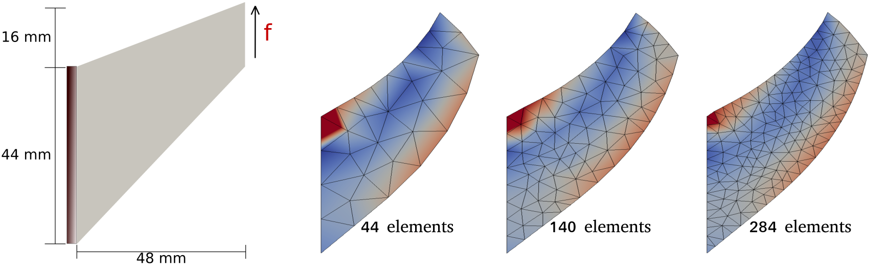
4.3 D Cook’s Membrane
Consider the D Cook’s membrane problem with the geometry shown in Figure 5. This example is usually used to study the performance in bending and in the near-incompressible regime [27]. The material properties are , and .
Figure 5 shows deformed configurations calculated using the element and the load . Colors in the deformed configurations depict the distribution of the Frobenius norm of stress . Figure 6 shows the convergence of the -norms of approximate solutions. Results are calculated using the elements and with two different loads of magnitudes and . These results suggest that the mixed formulation (2.4) can provide accurate approximations of stress in bending and in the near-compressible regime.

4.4 Inhomogeneous Compression
Enhanced strain methods are nonconformal three-field methods for small and finite deformations [8]. It is well-known that in some cases, these methods may become unstable due to the so-called hourglass instability [27]. One example for this type of instability is the inhomogeneous compression problem shown in Figure 7. The horizontal displacement at the top of the domain and the vertical displacement at the bottom are assumed to be zero and the material properties are the same as the previous example.
Deformed configurations of this problem associated to two different meshes which are calculated using the elements and the load are shown in Figure 7. Colors in the deformed configurations show the distribution of the Frobenius norm of stress. Figure 8 depicts the percentage of compression versus the number of elements for different loads . The compression level is calculated using the vertical displacement of the point of Figure 7, which is located at the midpoint of the top boundary. The results are consistent with those of [27]. Figure 9 shows the convergence of the -norm of solutions by refining meshes. We do not observe any numerical instability in our computations.

| FEM | DoF | FEM | DoF | ||||||||||||
|---|---|---|---|---|---|---|---|---|---|---|---|---|---|---|---|
| 735 | 1.82e-2 | 1.21e-1 | 1.67e-1 | 1887 | 1.86e-2 | 1.20e-1 | 1.61e-1 | ||||||||
| 4779 | 4.43e-3 | 6.35e-2 | 8.97e-2 | 13419 | 4.67e-3 | 6.23e-2 | 8.01e-2 | ||||||||
| 8943 | 2.79e-3 | 5.12e-2 | 7.28e-2 | 25593 | 2.96e-3 | 5.01e-2 | 6.36e-2 | ||||||||
| 1749 | 1.82e-2 | 1.21e-1 | 1.67e-1 | 2901 | 1.86e-2 | 1.20e-1 | 1.61e-1 | ||||||||
| 11775 | 4.43e-3 | 6.35e-2 | 8.97e-2 | 20415 | 4.67e-3 | 6.23e-2 | 8.01e-2 | ||||||||
| 22188 | 2.79e-3 | 5.12e-2 | 7.28e-2 | 38838 | 2.96e-3 | 5.01e-2 | 6.36e-2 | ||||||||
| 1455 | 1.83e-2 | 1.20e-1 | 1.57e-1 | 3399 | 1.86e-2 | 1.20e-1 | 1.63e-1 | ||||||||
| 9963 | 4.51e-3 | 6.26e-2 | 7.68e-2 | 24651 | 4.71e-3 | 6.23e-2 | 8.19e-2 | ||||||||
| 18843 | 2.84e-3 | 5.03e-2 | 6.05e-2 | 47193 | 2.99e-3 | 5.00e-2 | 6.51e-2 | ||||||||
| 2469 | 1.83e-2 | 1.20e-1 | 1.57e-1 | 4413 | 1.86e-2 | 2.00e-1 | 1.63e-1 | ||||||||
| 16959 | 4.51e-3 | 6.26e-2 | 7.68e-2 | 31647 | 4.71e-3 | 6.23e-2 | 8.19e-2 | ||||||||
| 32088 | 2.84e-3 | 5.03e-2 | 6.05e-2 | 60438 | 2.99e-3 | 5.00e-2 | 6.51e-2 | ||||||||
| 1029 | 1.82e-2 | 1.21e-1 | 1.67e-1 | 2181 | 1.86e-2 | 1.20e-1 | 1.61e-1 | ||||||||
| 6591 | 4.43e-3 | 6.35e-2 | 8.97e-2 | 15231 | 4.67e-3 | 6.23e-2 | 8.01e-2 | ||||||||
| 12288 | 2.79e-3 | 5.12e-2 | 7.28e-2 | 28938 | 2.96e-3 | 5.01e-2 | 6.36e-2 | ||||||||
| 2403 | 1.82e-2 | 1.21e-1 | 1.67e-1 | 3555 | 1.86e-2 | 1.20e-1 | 1.61e-1 | ||||||||
| 16179 | 4.43e-3 | 6.35e-2 | 8.97e-2 | 24819 | 4.67e-3 | 6.23e-2 | 8.01e-2 | ||||||||
| 30483 | 2.79e-3 | 5.12e-2 | 7.28e-2 | 47133 | 2.96e-3 | 5.01e-2 | 6.36e-2 | ||||||||
| 1749 | 1.83e-2 | 1.20e-1 | 1.57e-1 | 3693 | 1.86e-2 | 1.20e-1 | 1.63e-1 | ||||||||
| 11775 | 4.51e-3 | 6.26e-2 | 7.68e-2 | 26463 | 4.71e-3 | 6.23e-2 | 8.19e-2 | ||||||||
| 22188 | 2.84e-3 | 5.03e-2 | 6.05e-2 | 50538 | 2.99e-3 | 5.00e-2 | 6.51e-2 | ||||||||
| 3123 | 1.83e-2 | 1.20e-1 | 1.57e-1 | 5067 | 1.86e-2 | 1.20e-1 | 1.63e-1 | ||||||||
| 21363 | 4.51e-3 | 6.26e-2 | 7.68e-2 | 36051 | 4.71e-3 | 6.23e-2 | 8.19e-2 | ||||||||
| 40383 | 2.84e-3 | 5.03e-2 | 6.05e-2 | 68733 | 2.99e-3 | 5.00e-2 | 6.51e-2 | ||||||||
| 2475 | 1.30e-3 | 1.71e-2 | 2.41e-2 | 3987 | 1.30e-3 | 1.71e-2 | 2.40e-2 | ||||||||
| 17043 | 1.66e-4 | 4.37e-3 | 6.16e-3 | 28275 | 1.66e-4 | 4.34e-3 | 6.13e-3 | ||||||||
| 32283 | 8.65e-5 | 2.88e-3 | 4.33e-3 | 53883 | 8.54e-5 | 2.79e-3 | 3.94e-3 | ||||||||
| 3195 | 1.30e-3 | 1.71e-2 | 2.41e-2 | 4707 | 1.30e-3 | 1.70e-2 | 2.40e-2 | ||||||||
| 22227 | 1.66e-4 | 4.36e-3 | 6.16e-3 | 33459 | 1.66e-4 | 4.34e-3 | 6.13e-3 | ||||||||
| 42183 | 8.65e-5 | 2.88e-3 | 4.33e-3 | 63783 | 8.54e-5 | 2.79e-3 | 3.94e-3 | ||||||||
| 3849 | 1.30e-3 | 1.71e-2 | 2.41e-2 | 5361 | 1.30e-3 | 1.70e-2 | 2.40e-2 | ||||||||
| 26631 | 1.66e-4 | 4.36e-3 | 6.16e-3 | 37863 | 1.66e-4 | 4.34e-3 | 6.13e-3 | ||||||||
| 50478 | 8.65e-5 | 2.88e-3 | 4.33e-3 | 72078 | 8.54e-5 | 2.79e-3 | 3.94e-3 |


4.5 Deformation of a Cube
To study the convergence rates in the D case, we study the D analogue of the plate problem of Section 4.2. More specifically, we consider the unit cube with the material parameters and solve the mixed method (2.4) by using the body force and the boundary conditions that induce the displacement field
| (4.2) |
Table 2 shows -errors and convergence rates of the solutions of (2.4), which are calculated by using different combinations of the D elements of degrees 1 and 2 of Figure 1 and the structured meshes shown in the first row of Figure 10. Similar to the D plate example, one observes that the degree of the element for displacement has a significant effect on the overall performance of these mixed finite element methods. Moreover, Table 2 suggests that the convergence rates of displacement gradient and stress may not be optimal.
Our numerical results suggest that similar to D cases, combinations out of possible combinations of the D elements of Figure 1 are stable. The unstable cases are the same as those of D cases and are those that do not satisfy the inf-sup conditions (3.9) and (3.10). The extension of the mixed formulation (2.4) to the D case is straightforward. This is the main advantage of this formulation comparing to the mixed formulation of [9].
For the brevity, we consider the choices and in the remainder of this work. Figure 11 depicts the -errors of approximate solutions corresponding to the structured and unstructured meshes of Figure 10. The slopes of curves of the structured meshes are the convergence rates of Table 2. As the D case, these results suggest that mesh irregularities have more impact on the accuracy of approximate stresses.
4.6 A Near-Incompressible Cook-Type Beam
Next, we study the D analogue of Cook’s membrane under in-plane and out-of-plane loads. The geometry of this problem in the -plane is similar to that of the D case shown in Figure 5 with the thickness in the -direction, see Figure 12. We use the near-incompressible material properties of the D Cook’s membrane.
The configuration in the right panel of the first row of Figure 12 is the deformed configuration under a uniform load imposed at the right end of the beam in the -direction. The second row of Figure 12 shows two different angles of view of a deformed configuration due to the out-of-plane load in the -direction applied at the right end of the beam. These results are computed using and colors in the deformed configurations depict the distribution of the Frobenius norm of stress. Figure 13 shows the convergence of the -norms of finite element solutions associated to the above in-plane and out-of-plane loads. The elements and were used for these computations. Our results suggest that similar to the D case, the D mixed formulation (2.4) can provide accurate approximations of stress in bending and in the near-compressible regime.
5 Conclusion
We introduced a new mixed formulation for D and D nonlinear elasticity in terms of displacement, displacement gradient, and the first Piola-Kirchhoff stress tensor. We showed that even for hyperelastic solids, this formulation does not correspond to a stationary point of any functional, in general. For obtaining conformal mixed finite element methods based on this formulation, finite element spaces suitable for the and the operators are respectively employed for displacement gradient and stress. Discrete displacement gradients and stresses satisfy suitable jump conditions due to these choices.
We studied stability of these mixed finite element methods by writing suitable inf-sup conditions. We examined the performance of these methods for combinations of D and D simplicial elements of degree and and showed that combinations are not stable as they violate the inf-sup conditions. Several D and D numerical examples were solved to study convergence rates, the effect of mesh distortions, and the performance for bending problems and the near-incompressible regime. These examples suggest that it is possible to achieve the optimal convergence rates and obtain accurate approximations of strains and stresses. Moreover, we did not observe the hourglass instability that may occur in enhanced strain methods.
Appendix A An Abstract Theory for the Galerkin Approximation
In the following, we summarize the general framework for the Galerkin approximation of nonlinear problems introduced in [14, 15]. Let be a mapping, where and are Banach spaces with the norms and , respectively, and is the dual space of . Also let the linear operator be the (Fréchet) derivative of at , i.e. , . The goal is to approximate a regular solution of the problem , where regular means the derivative of at is “nonzero” in the sense that the linear mapping is one-to-one and onto. The relation is equivalent to
| (A.1) |
where , . Given finite element spaces and , a Galerkin approximation of the problem (A.1) reads: Find such that
| (A.2) |
To express sufficient conditions for the existence and the convergence of solutions of (A.2) as , we consider the bilinear form defined as
| (A.3) |
Then, one can show that the following result holds [15, Theorem 7.1]: Roughly speaking, for sufficiently small , the problem (A.2) has a unique solution in a neighborhood of a regular solution of (A.1) and as if: (i) Any element of can be approximated by as (approximibility); (ii) ; and (iii) There exists a mesh-independent number such that the following inf-sup condition holds:
| (A.4) |
It is also possible to write a priori and a posteriori estimates for the error [15, Theorem 7.1]. In particular, the a priori estimate provides an upper bound for which is proportional to . If the constant of the inf-sup condition is a mesh-dependent number such that as , then may converge poorly or diverge as even if the inf-sup condition holds for all meshes. Since is a regular solution of (A.1), the linearized problem
has a unique solution for any . The inf-sup condition (A.4) together with the condition (ii) imply that the discrete linear problem
| (A.5) |
also has a unique solution for any .
A simple approach to numerically investigate the inf-sup condition (A.4) is as follows: Let and respectively be global shape functions for and . Then, we have , , and , . We associate the vector () to () and define (). Assume that there exist symmetric and positive definite matrices and such that
By using the vectors and , the inf-sup condition (A.4) can be expressed in the matrix form
| (A.6) |
where the matrix is given by . Recall that the singular values of an arbitrary matrix are the square root of the eigenvalues of . Then, one can show that the inf-sup condition (A.4) holds if and only if the smallest singular value of is positive and bounded from below by a positive constant as [5, Proposition 3.4.5].
References
- Truesdell and Noll [1965] C. Truesdell and W. Noll. The Non-linear Field Theories of Mechanics. Springer, Berlin, 1965.
- Auricchio et al. [2013] F. Auricchio, L. da Veiga Beirao, C. Lovadina, A. Reali, R. L. Taylor, and P. Wriggers. Approximation of incompressible large deformation elastic problems: Some unresolved issues. Comput. Mech., 52:1153–1167, 2013.
- Auricchio et al. [2005] F. Auricchio, L. da Veiga Beirao, C. Lovadina, and A. Reali. A stability study of some mixed finite elements for large deformation elasticity problems. Comput. Methods Appl. Mech. Engrg., 194:1075–1092, 2005.
- Wriggers [2009] P. Wriggers. Mixed finite element methods - theory and discretization. In Mixed finite element technologies, pages 131–177. CISM Courses and Lectures, Springer-Verlag, Wien, 2009.
- Boffi et al. [2013] D. Boffi, F. Brezzi, and M. Fortin. Mixed Finite Element Methods and Applications. Springer-Verlag, Berlin, 2013.
- Oden [1972] J. T. Oden. Generalized conjugate functions for mixed finite element approximations of boundary value problems. In A. K. Aziz, editor, The Mathematical Foundations of the Finite Element Method with Applications to Partial Differential Equations, pages 629–669. Academic Press, New York, 1972.
- Ciarlet [1978] P. G. Ciarlet. The Finite Element Method for Elliptic Problems. North-Holland Publishing Co., Amsterdam, 1978.
- Simo and Armero [1992] J. C. Simo and F. Armero. Geometrically non-linear enhanced strain mixed methods and the method of incompatible modes. Int. J. Num. Methods Eng., 33:1413–1449, 1992.
- Angoshtari et al. [2017] A. Angoshtari, M. Faghih Shojaei, and A. Yavari. Compatible-Strain Mixed Finite Element Methods for 2D compressible nonlinear elasticity. Comput. Methods Appl. Mech. Engrg., 313:596–631, 2017.
- Reddy [2015] B. D. Reddy. Three-field mixed finite element methods in elasticity. In P. Wriggers and J. Schröder, editors, Advanced Finite Element Technologies, pages 53–68. Springer, Wien, 2015.
- Angoshtari and Yavari [2015] A. Angoshtari and A. Yavari. Differential complexes in continuum mechanics. Arch. Rational Mech. Anal., 216:193–220, 2015.
- Angoshtari and Yavari [2016] A. Angoshtari and A. Yavari. Hilbert complexes of nonlinear elasticity. Z. Angew. Math. Phys., 67:143, 2016.
- Wriggers and Reese [1996] P. Wriggers and S. Reese. A note on enhanced strain methods for large deformations. Comput. Methods Appl. Mech. Engrg., 135:201–209, 1996.
- Pousin and Rappaz [1994] J. Pousin and J. Rappaz. Consistency, stability, a priori and a posteriori errors for Petrov-Galerkin methods applied to nonlinear problems. Numer. Math., 69:213–231, 1994.
- Caloz and Rappaz [1997] G. Caloz and J. Rappaz. Numerical analysis for nonlinear and bifurcation problems. Handbook of numerical analysis, 5:487–637, 1997.
- Avez [1986] A. Avez. Differential Calculus. J. Wiley, New York, 1986.
- Angoshtari [2018] A. Angoshtari. On the impossibility of arbitrary deformations in nonlinear elasticity. Z. Angew. Math. Phys., 69:1, 2018.
- Arnold et al. [2010] D. N. Arnold, R. S. Falk, and R. Winther. Finite element exterior calculus: From Hodge theory to numerical stability. Bul. Am. Math. Soc., 47:281–354, 2010.
- Arnold et al. [2006] D. N. Arnold, R. S. Falk, and R. Winther. Finite element exterior calculus, homological techniques, and applications. Acta Numerica, 15:1–155, 2006.
- Logg et al. [2012] A. Logg, K. A. Mardal, and G. Wells. Automated Solution of Differential Equations by the Finite Element Method: The FEniCS Book, volume 84. Springer Science & Business Media, 2012.
- Nédélec [1986] J. C. Nédélec. A new family of mixed finite elements in . Numer. Math., 50:57–81, 1986.
- Brezzi et al. [1985] F. Brezzi, J. Douglas, Jr., and L. D. Marini. Two families of mixed finite elements for second order elliptic problems. Numer. Math., 47:217–235, 1985.
- Raviart and Thomas [1977] P. A. Raviart and J. M. Thomas. A mixed finite element method for 2nd order elliptic problems. In Mathematical aspects of finite element methods (Proc. Conf., Consiglio Naz. delle Ricerche (C.N.R.), Rome, 1975), pages 292–315. Vol. 606 of Lecture Notes in Mathematics, Springer, Berlin, 1977.
- Brezzi et al. [1981] F. Brezzi, J. Rappaz, and P. A. Raviart. Finite dimensional approximation of nonlinear problems. Simple bifurcation points. Numer. Math., 38:1–30, 1981.
- Ern and Guermond [2004] A. Ern and J. Guermond. Theory and Practice of Finite Elements. Springer-Verlag, New York, 2004.
- Ciarlet [1988] P. G. Ciarlet. Mathematical Elasticity, Vol I, Three Dimensional Elasticity. Elsevier, Amsterdam, 1988.
- Reese [2002] S. Reese. On the equivalence of mixed element formulations and the concept of reduced integration in large deformation problems. Int. J. Nonlin. Sci. Num., 3:1–33, 2002.