跳到论文正文
W Papers独立论文阅读器 arXiv:1910.08957 论文正文 计算阅读时间 · 0%
引用这篇论文根据当前论文元数据生成,正式投稿前建议核对。


License: arXiv.org perpetual non-exclusive license
arXiv:1910.08957v2 [math.CA] 19 Feb 2020

Asymptotic expansion of the modified exponential integral involving the Mittag-Leffler function

R. B. Paris Note: E-mail address: r.paris@abertay.ac.uk Affiliation: Division of Computing and Mathematics, Affiliation: Abertay University, Dundee DD1 1HG, UK
Abstract

We consider the asymptotic expansion of the generalised exponential integral involving the Mittag-Leffler function introduced recently by Mainardi and Masina [Fract. Calc. Appl. Anal. 21 (2018) 1156–1169]. We extend the definition of this function using the two-parameter Mittag-Leffler function. The expansions of the similarly extended sine and cosine integrals are also discussed. Numerical examples are presented to illustrate the accuracy of each type of expansion obtained.

MSC: 30E15, 30E20, 33E20, 34E05

Keywords: asymptotic expansions, exponential integral, Mittag-Leffler function, sine and cosine inegrals


1. Introduction

The complementary exponential integral Ein​(z)\hbox{Ein}(z) is defined by

Ein​(z)=∫0z1−e−tt​𝑑t=∑n=1∞(−)n−1​znn​n!(z∈𝐂)\hbox{Ein}(z)=\int_{0}^{z}\frac{1-e^{-t}}{t}\,dt=\sum_{n=1}^{\infty}\frac{(-)^{n-1}z^{n}}{nn!}\ \ \ (z\in\bf{C}) (1.1)

and is an entire function. Its connection with the classical exponential integral ℰ1​(z)=∫z∞t−1​e−t​𝑑t{\cal E}_{1}(z)=\int_{z}^{\infty}t^{-1}e^{-t}\,dt, valid in the cut plane |arg⁡z|<π|\arg\,z|<\pi, is [4, p. 150]

Ein​(z)=log⁡z+γ+ℰ1​(z),\hbox{Ein}(z)=\log\,z+\gamma+{\cal E}_{1}(z), (1.2)

where γ=0.5772156​…\gamma=0.5772156\dots is the Euler-Mascheroni constant.

In a recent paper, Mainardi and Masina [2] proposed an extension of Ein​(z)\hbox{Ein}(z) by replacing the exponential function in (1.1) by the one-parameter Mittag-Leffler function

Eα(z)=∑n=0∞znΓ⁡(α​n+1)(z∈𝐂,α>0),E_{\alpha}(z)=\sum_{n=0}^{\infty}\frac{z^{n}}{\Gamma(\alpha n+1)}\qquad(z\in{\bf C},\ \ \alpha>0),

which generalises the exponential function eze^{z}. They introduced the function for any α>0\alpha>0 in the cut plane |arg⁡z|<π|\arg\,z|<\pi

Einα​(z)=∫0z1−Eα​(−tα)tα​𝑑t=∑n=0∞(−)n​zα​n+1(α​n+1)​Γ​(α​n+α+1),\hbox{Ein}_{\alpha}(z)=\int_{0}^{z}\frac{1-E_{\alpha}(-t^{\alpha})}{t^{\alpha}}\,dt=\sum_{n=0}^{\infty}\frac{(-)^{n}z^{\alpha n+1}}{(\alpha n+1)\Gamma(\alpha n+\alpha+1)}, (1.3)

which when α=1\alpha=1 reduces to the function Ein​(z)\hbox{Ein}(z). A physical application of this function for 0≤α≤10\leq\alpha\leq 1 arises in the study of the creep features of a linear viscoelastic model; see [3] for details. An analogous extension of the generalised sine and cosine integrals was also considered in [2]. Plots of all these functions for α∈[0,1]\alpha\in[0,1] were given.

Here we consider a slightly more general version of (1.3) based on the two-parameter Mittag-Leffler function given by

Eα,β​(z)=∑n=0∞znΓ⁡(α​n+β)(z∈𝐂,α>0),E_{\alpha,\beta}(z)=\sum_{n=0}^{\infty}\frac{z^{n}}{\Gamma(\alpha n+\beta)}\qquad(z\in{\bf C},\ \alpha>0),

where β\beta will be taken to be real. Then the extended complementary exponential integral we shall consider is

Einα,β​(z)=∫0z1−Eα,β​(−tα)tα​𝑑t=∑n=1∞(−)n−1Γ⁡(α​n+β)​∫0ztα​n−α​𝑑t\hbox{Ein}_{\alpha,\beta}(z)=\int_{0}^{z}\frac{1-E_{\alpha,\beta}(-t^{\alpha})}{t^{\alpha}}\,dt=\sum_{n=1}^{\infty}\frac{(-)^{n-1}}{\Gamma(\alpha n+\beta)}\int_{0}^{z}t^{\alpha n-\alpha}dt
=z​∑n=0∞(−)n​zα​n(α​n+1)​Γ​(α​n+α+β)=z\sum_{n=0}^{\infty}\frac{(-)^{n}z^{\alpha n}}{(\alpha n+1)\Gamma(\alpha n+\alpha+\beta)}\hskip 56.9055pt (1.4)

upon replacement of n−1n-1 by nn in the last summation. When β=1\beta=1 this reduces to (1.3) so that Einα,1​(z)=Einα​(z)\hbox{Ein}_{\alpha,1}(z)=\hbox{Ein}_{\alpha}(z).

The asymptotic expansion of this function will be obtained for large complex zz with the parameters α\alpha, β\beta held fixed. We achieve this by consideration of the asymptotics of a related function using the theory developed for integral functions of hypergeometric type as discussed, for example, in [7, §2.3]. An interesting feature of the expansion of Einα,β​(x)\hbox{Ein}_{\alpha,\beta}(x) for x→+∞x\to+\infty when α∈(0,1]\alpha\in(0,1] is the appearance of a logarithmic term whenever α=1,12,13,…\alpha=1,\hbox{${\textstyle\frac{1}{2}}$},\hbox{${\textstyle\frac{1}{3}}$},\ldots\ . Similar expansions are obtained for the extended sine and cosine integrals in Section 4. The paper concludes with the presentation of some numerical results that demonstrate the accuracy of the different expansions obtained.

2. The asymptotic expansion of a related function for |z|→∞|z|\to\infty

To determine the asymptotic expansion of Einα,β​(z)\hbox{Ein}_{\alpha,\beta}(z) for large complex zz with the parameters α\alpha and β\beta held fixed, we shall find it convenient to consider the related function defined by

F⁡(χ):=∑n=0∞χn(α​n+γ)​Γ​(α​n+α+β)=∑n=0∞g⁡(n)​χnn!(χ∈𝐂),F(\chi):=\sum_{n=0}^{\infty}\frac{\chi^{n}}{(\alpha n+\gamma)\Gamma(\alpha n+\alpha+\beta)}=\sum_{n=0}^{\infty}g(n)\frac{\chi^{n}}{n!}\qquad(\chi\in{\bf C}), (2.1)

where

g⁡(n)=Γ⁡(n+1)(α​n+γ)​Γ​(α​n+α+β)=Γ⁡(α​n+γ)​Γ​(n+1)Γ⁡(α​n+γ+1)​Γ​(α​n+α+β).g(n)=\frac{\Gamma(n+1)}{(\alpha n+\gamma)\Gamma(\alpha n+\alpha+\beta)}=\frac{\Gamma(\alpha n+\gamma)\Gamma(n+1)}{\Gamma(\alpha n+\gamma+1)\Gamma(\alpha n+\alpha+\beta)}~.

The parameter γ>0\gamma>0, but will be chosen to have two specific values in Sections 3 and 4; namely, γ=1\gamma=1 and γ=1+α\gamma=1+\alpha. It will be shown that the asymptotic expansion of F⁡(χ)F(\chi) consists of an algebraic and an exponential expansion valid in different sectors of the complex χ\chi-plane.

The function F⁡(χ)F(\chi) in (2.1) is a case of the Wright function

Ψqp​(χ)=∑n=0∞∏r=1pΓ⁡(αr​n+ar)∏r=1qΓ⁡(βr​n+br)​χnn!,{}_{p}\Psi_{q}(\chi)=\sum_{n=0}^{\infty}\frac{\prod_{r=1}^{p}\Gamma(\alpha_{r}n+a_{r})}{\prod_{r=1}^{q}\Gamma(\beta_{r}n+b_{r})}\,\frac{\chi^{n}}{n!}, (2.2)

corresponding to p=q=2p=q=2. In (2.2) the parameters αr\alpha_{r} and βr\beta_{r} are real and positive and ara_{r} and brb_{r} are arbitrary complex numbers. We also assume that the αr\alpha_{r} and ara_{r} are subject to the restriction

αrn+ar≠0,−1,−2,…(n=0,1,2,…; 1≤r≤p)\alpha_{r}n+a_{r}\neq 0,-1,-2,\ldots\qquad(n=0,1,2,\ldots\ ;\,1\leq r\leq p)

so that no gamma function in the numerator in (2.2) is singular. The parameters associated11 1 Empty sums and products are to be interpreted as zero and unity, respectively. with Ψqp​(χ){}_{p}\Psi_{q}(\chi) are given by

κ=1+∑r=1qβr−∑r=1pαr,h=∏r=1pαrαr​∏r=1qβr−βr,\kappa=1+\sum_{r=1}^{q}\beta_{r}-\sum_{r=1}^{p}\alpha_{r},\qquad h=\prod_{r=1}^{p}\alpha_{r}^{\alpha_{r}}\prod_{r=1}^{q}\beta_{r}^{-\beta_{r}},
ϑ=∑r=1par−∑r=1qbr+12​(q−p),ϑ′=1−ϑ.\vartheta=\sum_{r=1}^{p}a_{r}-\sum_{r=1}^{q}b_{r}+\hbox{${\textstyle\frac{1}{2}}$}(q-p),\qquad\vartheta^{\prime}=1-\vartheta. (2.3)

The algebraic expansion of F⁡(χ)F(\chi) is obtained from the Mellin-Barnes integral representation [7, p. 56]

F⁡(χ)=12​π​i​∫c−∞​ic+∞​iΓ⁡(−s)​Γ​(1+s)​(χ​e∓π​i)s(α​s+γ)​Γ​(α​s+α+β)​𝑑s,|arg⁡(−χ)|<π⁡(1−12​α),F(\chi)=\frac{1}{2\pi i}\int_{c-\infty i}^{c+\infty i}\frac{\Gamma(-s)\Gamma(1+s)(\chi e^{\mp\pi i})^{s}}{(\alpha s+\gamma)\Gamma(\alpha s+\alpha+\beta)}\,ds,\qquad|\arg(-\chi)|<\pi(1-\hbox{${\textstyle\frac{1}{2}}$}\alpha),

where, with −γ/α<c<0-\gamma/\alpha<c<0, the integration path lies to the left of the poles of Γ⁡(−s)\Gamma(-s) at s=0,1,2,…s=0,1,2,\ldots but to the right of the poles at s=−γ/αs=-\gamma/\alpha and s=−k−1s=-k-1, k=0,1,2,…k=0,1,2,\ldots\,. The upper or lower sign is taken according as arg⁡χ>0\arg\,\chi>0 or arg⁡χ<0\arg\,\chi<0, respectively. It is seen that when α=γ/m\alpha=\gamma/m, m=1,2,…m=1,2,\ldots the pole at s=−ms=-m is double and its residue must be evaluated accordingly. Displacement of the integration path to the left when 0<α<20<\alpha<2 and evaluation of the residues then produces the algebraic expansion H⁡(χ​e∓π​i)H(\chi e^{\mp\pi i}), where

H⁡(χ)={π/αsin⁡γ​π/α​χ−γ/αΓ⁡(α+β−γ)+∑k=0∞(−)k​χ−k−1(γ−α⁡(k+1))​Γ​(β−α​k)(α≠γm)(−)m−1​χ−mΓ⁡(α+β−γ)​{mγ​log⁡χ−ψ⁡(α+β−γ)}+∑k=0∞k≠m−1(−)k​χ−k−1(γ−α⁡(k+1))​Γ​(β−α​k)(α=γm),H(\chi)=\left\{\begin{array}[]{ll}\!\!\!\displaystyle{\frac{\pi/\alpha}{\sin\gamma\pi/\alpha}}\,\displaystyle{\frac{\chi^{-\gamma/\alpha}}{\Gamma(\alpha+\beta-\gamma)}}+\sum_{k=0}^{\infty}\displaystyle{\frac{(-)^{k}\chi^{-k-1}}{(\gamma-\alpha(k+1))\Gamma(\beta-\alpha k)}}&(\alpha\neq\displaystyle{\frac{\gamma}{m}})\\ \\ \!\!\!\displaystyle{\frac{(-)^{m-1}\chi^{-m}}{\Gamma(\alpha+\beta-\gamma)}}\biggl\{\frac{m}{\gamma}\log\,\chi-\psi(\alpha+\beta-\gamma)\biggr\}+\mathop{\sum_{k=0}^{\infty}}_{\scriptstyle k\neq m-1}\displaystyle{\frac{(-)^{k}\chi^{-k-1}}{(\gamma-\alpha(k+1))\Gamma(\beta-\alpha k)}}&(\alpha=\displaystyle{\frac{\gamma}{m}}),\end{array}\right. (2.4)

and ψ\psi denotes the logarithmic derivative of the gamma function.

The exponential expansion associated with Ψqp​(χ){}_{p}\Psi_{q}(\chi) is given by [6, p. 299], [7, p. 57]

ℰ⁡(χ):=Xϑ​eX​∑j=0∞Aj​X−j,X=κ​(h​χ)1/κ,{\cal E}(\chi):=X^{\vartheta}e^{X}\sum_{j=0}^{\infty}A_{j}X^{-j},\qquad X=\kappa(h\chi)^{1/\kappa}, (2.5)

where the coefficients AjA_{j} are those appearing in the inverse factorial expansion

1Γ⁡(1+s)​∏r=1pΓ⁡(αr​n+ar)∏r=1qΓ⁡(βr​n+br)=κ​A0​(h​κκ)s​{∑j=0M−1cjΓ⁡(κ​s+ϑ′+j)+ρM​(s)Γ⁡(κ​s+ϑ′+M)}\frac{1}{\Gamma(1+s)}\,\frac{\prod_{r=1}^{p}\Gamma(\alpha_{r}n+a_{r})}{\prod_{r=1}^{q}\Gamma(\beta_{r}n+b_{r})}=\kappa A_{0}(h\kappa^{\kappa})^{s}\biggl\{\sum_{j=0}^{M-1}\frac{c_{j}}{\Gamma(\kappa s+\vartheta^{\prime}+j)}+\frac{\rho_{M}(s)}{\Gamma(\kappa s+\vartheta^{\prime}+M)}\biggr\} (2.6)

with c0=1c_{0}=1. Here MM is a positive integer and ρM​(s)=O​(1)\rho_{M}(s)=O(1) for |s|→∞|s|\rightarrow\infty in |arg⁡s|<π|\arg\,s|<\pi. The constant A0A_{0} is specified by

A0=(2​π)12​(p−q)​κ−12−ϑ​∏r=1pαrar−12​∏r=1qβr12−br.A_{0}=(2\pi)^{\frac{1}{2}(p-q)}\kappa^{-\frac{1}{2}-\vartheta}\prod_{r=1}^{p}\alpha_{r}^{a_{r}-\frac{1}{2}}\prod_{r=1}^{q}\beta_{r}^{\frac{1}{2}-b_{r}}.

The coefficients cjc_{j} are independent of ss and depend only on the parameters pp, qq, αr\alpha_{r}, βr\beta_{r}, ara_{r} and brb_{r}.

For the function F⁡(χ)F(\chi), we have

κ=α,h=α−α,ϑ=−α−β,A0=α−1.\kappa=\alpha,\quad h=\alpha^{-\alpha},\quad\vartheta=-\alpha-\beta,\quad A_{0}=\alpha^{-1}.

We are in the fortunate position that the normalised coefficients cjc_{j} in this case can be determined explicitly as cj=(α+β−γ)jc_{j}=(\alpha+\beta-\gamma)_{j}. This follows from the well-known (convergent) expansion given in [1], [7, p. 41]

1(α​s+γ)​Γ​(α​s+α+β)=∑j=0∞(α+β−γ)jΓ⁡(α​s+ϑ′+j)(ℜ(s)>−γ/α),\frac{1}{(\alpha s+\gamma)\Gamma(\alpha s+\alpha+\beta)}=\sum_{j=0}^{\infty}\frac{(\alpha+\beta-\gamma)_{j}}{\Gamma(\alpha s+\vartheta^{\prime}+j)}\qquad(\Re(s)>-\gamma/\alpha), (2.7)

to which, in the case of F⁡(χ)F(\chi), the ratio of gamma functions appearing on the left-hand side of (2.6) reduces. Then, with X=χ1/αX=\chi^{1/\alpha} we have from (2.5) the exponential expansion associated with F⁡(χ)F(\chi) given by

ℰ(χ)=1αχϑ/αexp[χ1/α]∑j=0∞(α+β−γ)jχ−j/α.{\cal E}(\chi)=\frac{1}{\alpha}\chi^{\vartheta/\alpha}\exp\,[\chi^{1/\alpha}]\,\sum_{j=0}^{\infty}\,(\alpha+\beta-\gamma)_{j}\,\chi^{-j/\alpha}. (2.8)

From [7, pp. 57–58], we then obtain the asymptotic expansion for |χ|→∞|\chi|\to\infty when 0<α<20<\alpha<2

F⁡(χ)∼{ℰ⁡(χ)+H⁡(χ​e∓π​i)|arg⁡χ|<12​π​αH⁡(χ​e∓π​i)|arg⁡(−χ)|<π⁡(1−12​α)F(\chi)\sim\left\{\begin{array}[]{ll}{\cal E}(\chi)+H(\chi e^{\mp\pi i})&|\arg\,\chi|<\hbox{${\textstyle\frac{1}{2}}$}\pi\alpha\\ \\ H(\chi e^{\mp\pi i})&|\arg(-\chi)|<\pi(1-\hbox{${\textstyle\frac{1}{2}}$}\alpha)\end{array}\right. (2.9)

and, when α=2\alpha=2,

F⁡(χ)∼ℰ⁡(χ)+ℰ⁡(χ​e∓2​π​i)+H⁡(χ​e∓π​i)|arg⁡χ|≤π.F(\chi)\sim{\cal E}(\chi)+{\cal E}(\chi e^{\mp 2\pi i})+H(\chi e^{\mp\pi i})\qquad|\arg\,\chi|\leq\pi. (2.10)

The upper and lower signs are chosen according as arg⁡χ>0\arg\,\chi>0 or arg⁡χ<0\arg\,\chi<0, respectively. It may be noted that the expansions ℰ⁡(χ​e∓2​π​i){\cal E}(\chi e^{\mp 2\pi i}) in (2.10) only become significant in the neighbourhood of arg⁡χ=±π\arg\,\chi=\pm\pi. When α>2\alpha>2, the expansion of F⁡(χ)F(\chi) is exponentially large for all values of arg⁡χ\arg\,\chi (see [7, p. 58]) and accordingly we omit this case as it is unlikely to be of physical interest.

Remark 2.1 The exponential expansion ℰ⁡(χ){\cal E}(\chi) in (2.9) continues to hold beyond the sector |arg⁡χ|<12​π​α|\arg\,\chi|<\hbox{${\textstyle\frac{1}{2}}$}\pi\alpha, where it becomes exponentially small in the sectors π​α≤|arg⁡χ|<12​π​α\pi\alpha\leq|\arg\,\chi|<\hbox{${\textstyle\frac{1}{2}}$}\pi\alpha when 0<α≤10<\alpha\leq 1. The rays arg⁡χ=±π​α\arg\,\chi=\pm\pi\alpha are Stokes lines, where ℰ⁡(χ){\cal E}(\chi) is maximally subdominant relative to the algebraic expansion H⁡(χ​e∓π​i)H(\chi e^{\mp\pi i}). On these rays, ℰ⁡(χ){\cal E}(\chi) undergoes a Stokes phenomenon, where the exponentially small expansion “switches off” in a smooth manner as |arg⁡χ||\arg\,\chi| increases [4, §2.11(iv)], with its value to leading order given by 12​ℰ​(χ)\hbox{${\textstyle\frac{1}{2}}$}{\cal E}(\chi); see [5] for a more detailed discussion of this point in the context of the confluent hypergeometric functions. We do not consider exponentially small contributions to F⁡(χ)F(\chi) here, except to briefly mention in Section 3 the situation pertaining to the case α=1\alpha=1.

3. The asymptotic expansion of Einα,β​(z)\hbox{Ein}_{\alpha,\beta}(z) for |z|→∞|z|\to\infty

The asymptotic expansion of Einα,β​(z)\hbox{Ein}_{\alpha,\beta}(z) defined in (1.4) can now be constructed from that of F⁡(χ)F(\chi) with the parameter γ=1\gamma=1. It is sufficient, for real α\alpha, β\beta, to consider 0≤arg⁡z≤π0\leq\arg\,z\leq\pi, since the expansion when arg⁡z<0\arg\,z<0 is given by the conjugate value. With χ=−zα=e−π​i​zα\chi=-z^{\alpha}=e^{-\pi i}z^{\alpha}, the exponentially large sector |arg⁡χ|<12​π​α|\arg\,\chi|<\hbox{${\textstyle\frac{1}{2}}$}\pi\alpha becomes |−π+α​arg⁡z|<12​π​α|-\pi+\alpha\arg\,z|<\hbox{${\textstyle\frac{1}{2}}$}\pi\alpha; that is

θ0<arg⁡z<θ0+π,θ0:=π2​α​(2−α).\theta_{0}<\arg\,z<\theta_{0}+\pi,\qquad\theta_{0}:=\frac{\pi}{2\alpha}(2-\alpha). (3.1)

On the boundaries of this sector the exponential expansion is of an oscillatory character. When 0<α<230<\alpha<\hbox{${\textstyle\frac{2}{3}}$}, we note that the exponentially large sector (3.1) lies outside the sector of interest 0≤arg⁡z≤π0\leq\arg\,z\leq\pi.

We define the algebraic and exponential asymptotic expansions

Hα,β​(z)={π/αsin⁡(π/α)​Γ​(α+β−1)+∑k=0∞(−)k​z1−α⁡(k+1)(1−α⁡(k+1))​Γ​(β−α​k)(α≠m−1)(−)m−1Γ⁡(α+β−1)​{log⁡z−ψ⁡(α+β−1)}+∑k=0∞k≠m−1(−)k​z1−α⁡(k+1)(1−α⁡(k+1))​Γ​(β−α​k)(α=m−1),H_{\alpha,\beta}(z)=\left\{\begin{array}[]{ll}\!\!\!\displaystyle{\frac{\pi/\alpha}{\sin(\pi/\alpha)\,\Gamma(\alpha+\beta-1)}}+\sum_{k=0}^{\infty}\displaystyle{\frac{(-)^{k}z^{1-\alpha(k+1)}}{(1-\alpha(k+1))\Gamma(\beta-\alpha k)}}&(\alpha\neq m^{-1})\\ \\ \!\!\!\displaystyle{\frac{(-)^{m-1}}{\Gamma(\alpha+\beta-1)}}\{\log\,z-\psi(\alpha+\beta-1)\}+\mathop{\sum_{k=0}^{\infty}}_{\scriptstyle k\neq m-1}\displaystyle{\frac{(-)^{k}z^{1-\alpha(k+1)}}{(1-\alpha(k+1))\Gamma(\beta-\alpha k)}}&(\alpha=m^{-1}),\end{array}\right. (3.2)

where m=1,2,…m=1,2,\ldots\,, and

ℰα,β(z)=(e−πi/αz)ϑαexp[e−πi/αz]∑j=0∞(α+β−1)j(e−πi/αz)−j{\cal E}_{\alpha,\beta}(z)=\frac{(e^{-\pi i/\alpha}z)^{\vartheta}}{\alpha}\,\exp\,[e^{-\pi i/\alpha}z]\sum_{j=0}^{\infty}(\alpha+\beta-1)_{j}(e^{-\pi i/\alpha}z)^{-j} (3.3)

where we recall that ϑ=−α−β\vartheta=-\alpha-\beta. Then the following result holds:

Theorem 1. Let mm be a positive integer, with α>0\alpha>0 and β\beta real and θ0=π⁡(2−α)/(2​α)\theta_{0}=\pi(2-\alpha)/(2\alpha). Then the following expansions hold for |z|→∞|z|\to\infty

Einα,β​(z)∼Hα,β​(z)(0≤arg⁡z≤π)\hbox{Ein}_{\alpha,\beta}(z)\sim H_{\alpha,\beta}(z)\qquad(0\leq\arg\,z\leq\pi) (3.4)

when 0<α<230<\alpha<\hbox{${\textstyle\frac{2}{3}}$}, and

Einα,β​(z)∼{Hα,β​(z)(0≤arg⁡z<θ0)z​ℰα,β​(z)+Hα,β​(z)(θ0≤arg⁡z≤π)\hbox{Ein}_{\alpha,\beta}(z)\sim\left\{\begin{array}[]{ll}H_{\alpha,\beta}(z)&(0\leq\arg\,z<\theta_{0})\\ \\ z{\cal E}_{\alpha,\beta}(z)+H_{\alpha,\beta}(z)&(\theta_{0}\leq\arg\,z\leq\pi)\end{array}\right. (3.5)

when 23≤α<2\hbox{${\textstyle\frac{2}{3}}$}\leq\alpha<2. Finally, when α=2\alpha=2 we have Ein2,β​(−z)=−Ein2,β​(z)\hbox{Ein}_{2,\beta}(-z)=-\hbox{Ein}_{2,\beta}(z) and it is therefore sufficient to consider 0≤arg⁡z≤12​π0\leq\arg\,z\leq\hbox{${\textstyle\frac{1}{2}}$}\pi. Then, from (2.10), we obtain the expansion when α=2\alpha=2

Ein2,β​(z)∼z⁡{ℰ2,β​(z)+ℰ2,β​(z​eπ​i)}+H2,β​(z)(0≤arg⁡z≤12​π).\hbox{Ein}_{2,\beta}(z)\sim z\{{\cal E}_{2,\beta}(z)+{\cal E}_{2,\beta}(ze^{\pi i})\}+H_{2,\beta}(z)\qquad(0\leq\arg\,z\leq\hbox{${\textstyle\frac{1}{2}}$}\pi). (3.6)

We note from Theorem 1 that when z→−∞z\to-\infty the value of Einα,β​(z)\hbox{Ein}_{\alpha,\beta}(z) is, in general, complex-valued.

In the case of main physical interest, when z=x>0z=x>0 is a real variable, we have the following expansion:

Theorem 2. When z=xz=x (>0)(>0) we have from Theorem 1 the expansions

Einα,β​(x)∼Hα,β​(x)\hbox{Ein}_{\alpha,\beta}(x)\sim H_{\alpha,\beta}(x) (3.7)

for 0<α<20<\alpha<2, and from (3.3) and (3.6) when α=2\alpha=2

Ein2,β​(x)∼H2,β​(x)−x−1−β​∑j=0∞(1+β)jxj​cos⁡[x−12​π​(β+j)]\hbox{Ein}_{2,\beta}(x)\sim H_{2,\beta}(x)-x^{-1-\beta}\sum_{j=0}^{\infty}\frac{(1+\beta)_{j}}{x^{j}}\,\cos\,[x-\hbox{${\textstyle\frac{1}{2}}$}\pi(\beta+j)] (3.8)

as x→+∞x\to+\infty.

It is worth noting that a logarithmic term is present in the asymptotic expansion of Einα,β​(x)\hbox{Ein}_{\alpha,\beta}(x) whenever α=1,12,13,…\alpha=1,\hbox{${\textstyle\frac{1}{2}}$},\hbox{${\textstyle\frac{1}{3}}$},\ldots\ .

3.1 The case α=1\alpha=1

The special case α=1\alpha=1 deserves further consideration. From (3.2) and (3.7) we obtain the expansion

Ein1,β​(x)∼1Γ⁡(β)​{log⁡x−ψ⁡(β)}−∑k=1∞(−x)−kk​Γ​(β−k)(x→+∞).\hbox{Ein}_{1,\beta}(x)\sim\frac{1}{\Gamma(\beta)}\{\log\,x-\psi(\beta)\}-\sum_{k=1}^{\infty}\frac{(-x)^{-k}}{k\,\Gamma(\beta-k)}\qquad(x\to+\infty). (3.9)

If β=1\beta=1, the asymptotic sum in (3.9) vanishes and

Ein1,1​(x)∼log⁡x+γ\hbox{Ein}_{1,1}(x)\sim\log\,x+\gamma (3.10)

for large xx. But we have the exact evaluation (compare (1.2))

Ein1,1​(x)=x​∑n=0∞(−x)n(n+1)2​n!=log⁡x+γ+ℰ1​(x)\hbox{Ein}_{1,1}(x)=x\sum_{n=0}^{\infty}\frac{(-x)^{n}}{(n+1)^{2}n!}=\log\,x+\gamma+{\cal E}_{1}(x)
∼logx+γ+e−xx∑j=0∞(−)j​j!xj(x→+∞)\hskip 68.28644pt\sim\log\,x+\gamma+\frac{e^{-x}}{x}\sum_{j=0}^{\infty}\frac{(-)^{j}j!}{x^{j}}\qquad(x\to+\infty) (3.11)

by [4, (6.12.1)]. The additional asymptotic sum appearing in (3.11) is exponentially small as x→+∞x\to+\infty and is consequently not accounted for in the result (3.10).

From Remark 2.1, it is seen that there are Stokes lines at arg⁡z=±π⁡(1−α)\arg\,z=\pm\pi(1-\alpha), which coalesce on the positive real axis when α=1\alpha=1. In the sense of increasing arg⁡z\arg\,z in the neighbourhood of the positive real axis, the exponential expansion ℰ1,β​(z){\cal E}_{1,\beta}(z) is in the process of switching on across arg⁡z=π⁡(1−α)\arg\,z=\pi(1-\alpha) and ℰ1,β​(z)¯\overline{{\cal E}_{1,\beta}(z)} (where the bar denotes the complex conjugate) is in the process of switching off across arg⁡z=−π⁡(1−α)\arg\,z=-\pi(1-\alpha). When α=1\alpha=1, this produces the exponential contribution

12​x​{ℰ1,β​(x)+ℰ1,β​(x)¯}=e−xxβ​cos⁡π​β​∑j=0∞(−)j+1​(β)jxj\hbox{${\textstyle\frac{1}{2}}$}x\{{\cal E}_{1,\beta}(x)+\overline{{\cal E}_{1,\beta}(x)}\}=\frac{e^{-x}}{x^{\beta}}\,\cos\pi\beta\,\sum_{j=0}^{\infty}\frac{(-)^{j+1}(\beta)_{j}}{x^{j}}

for large xx. Thus, the more accurate version of (3.9) should read

Ein1,β​(x)∼1Γ⁡(β)​{log⁡x−ψ⁡(β)}−∑k=1∞(−x)−kk​Γ​(β−k)−e−xxβ​cos⁡π​β​∑j=0∞(−)j​(β)jxj\hbox{Ein}_{1,\beta}(x)\sim\frac{1}{\Gamma(\beta)}\{\log\,x-\psi(\beta)\}-\sum_{k=1}^{\infty}\frac{(-x)^{-k}}{k\,\Gamma(\beta-k)}-\frac{e^{-x}}{x^{\beta}}\,\cos\pi\beta\,\sum_{j=0}^{\infty}\frac{(-)^{j}(\beta)_{j}}{x^{j}} (3.12)

as x→+∞x\to+\infty. When β=1\beta=1, this correctly reduces to (3.11).

When β=2\beta=2, we have [8]

Ein1,2​(x)=x​∑n=0∞(−x)n(n+1)2​(n+2)​n!=log⁡x−ψ⁡(2)+1x+ℰ1​(x)−e−xx\hbox{Ein}_{1,2}(x)=x\sum_{n=0}^{\infty}\frac{(-x)^{n}}{(n+1)^{2}(n+2)n!}=\log\,x-\psi(2)+\frac{1}{x}+{\cal E}_{1}(x)-\frac{e^{-x}}{x}
∼logx−ψ(2)+1x+e−xx∑j=1∞(−)j​j!xj(x→+∞).\hskip 11.38092pt\sim\log\,x-\psi(2)+\frac{1}{x}+\frac{e^{-x}}{x}\sum_{j=1}^{\infty}\frac{(-)^{j}j!}{x^{j}}\qquad(x\to+\infty).

This can be seen also to agree with (3.12) after a little rearrangement.

4. The generalised sine and cosine integrals

The sine and cosine integrals are defined by [4, §6.2]

Si​(z)=∫0zsin⁡tt​𝑑t,Cin​(z)=∫0z1−cos⁡tt​𝑑t.\hbox{Si}(z)=\int_{0}^{z}\frac{\sin t}{t}\,dt,\qquad\hbox{Cin}(z)=\int_{0}^{z}\frac{1-\cos t}{t}\,dt.

Mainardi and Masina [2] generalised these definitions by replacing the trigonometric functions by

sinα⁡(t)=tα​E2​α,α+β​(−t2​α)=∑n=0∞(−)n​t(2​n+1)​αΓ⁡(2​n​α+α+β),cosα⁡(t)=E2​α,β​(−t2​α)=∑n=0∞(−)n​t2​n​αΓ⁡(2​n​α+β)\sin_{\alpha}(t)=t^{\alpha}E_{2\alpha,\alpha+\beta}(-t^{2\alpha})=\sum_{n=0}^{\infty}\frac{(-)^{n}t^{(2n+1)\alpha}}{\Gamma(2n\alpha+\alpha+\beta)},\quad\cos_{\alpha}(t)=E_{2\alpha,\beta}(-t^{2\alpha})=\sum_{n=0}^{\infty}\frac{(-)^{n}t^{2n\alpha}}{\Gamma(2n\alpha+\beta)}

with β=1\beta=1 to produce

{Sinα​(z)=∫0zsinα⁡(t)tα​𝑑t=∑n=0∞(−)n​z2​n​α+1(2​n​α+1)​Γ​(2​n​α+α+1)Cinα​(z)=∫0∞1−cosα⁡(t)tα​dt=∑n=0∞(−)n​z2​n​α+α+1(2​n​α+α+1)​Γ​(2​n​α+2​α+1).\left\{\begin{array}[]{l}\hbox{Sin}_{\alpha}(z)={\displaystyle\int_{0}^{z}\displaystyle{\frac{\sin_{\alpha}(t)}{t^{\alpha}}}\,dt=\sum_{n=0}^{\infty}\displaystyle{\frac{(-)^{n}z^{2n\alpha+1}}{(2n\alpha+1)\Gamma(2n\alpha+\alpha+1)}}}\\ \\ \hbox{Cin}_{\alpha}(z)={\displaystyle\int_{0}^{\infty}\displaystyle{\frac{1-\cos_{\alpha}(t)}{t^{\alpha}}}\,dt=\sum_{n=0}^{\infty}\displaystyle{\frac{(-)^{n}z^{2n\alpha+\alpha+1}}{(2n\alpha+\alpha+1)\Gamma(2n\alpha+2\alpha+1)}}}~.\end{array}\right. (4.1)

Here we extend the definitions (4.1) by including the additional parameter β∈𝐑\beta\in{\bf R} in the Mittag-Leffler functions and consider the functions

{Sinα,β​(z)=z​∑n=0∞(−)n​z2​n​α(2​n​α+1)​Γ​(2​n​α+α+β)Cinα,β​(z)=z1+α​∑n=0∞(−)n​z2​n​α(2​n​α+α+1)​Γ​(2​n​α+2​α+β).\left\{\begin{array}[]{l}\hbox{Sin}_{\alpha,\beta}(z)={\displaystyle z\sum_{n=0}^{\infty}\displaystyle{\frac{(-)^{n}z^{2n\alpha}}{(2n\alpha+1)\Gamma(2n\alpha+\alpha+\beta)}}}\\ \\ \hbox{Cin}_{\alpha,\beta}(z)={\displaystyle z^{1+\alpha}\sum_{n=0}^{\infty}\displaystyle{\frac{(-)^{n}z^{2n\alpha}}{(2n\alpha+\alpha+1)\Gamma(2n\alpha+2\alpha+\beta)}}}~.\end{array}\right. (4.2)

The asymptotics of Sinα,β​(z)\hbox{Sin}_{\alpha,\beta}(z) and Cinα,β​(z)\hbox{Cin}_{\alpha,\beta}(z) can be deduced from the results in Section 2. However, here we restrict ourselves to determining the asymptotic expansion of these functions for large |z||z| in a sector enclosing the positive real zz-axis, where for 0<α<10<\alpha<1 they only have an algebraic-type expansion. We observe in passing that

Sinα,β​(z)=Ein2​α,β−α​(z).\hbox{Sin}_{\alpha,\beta}(z)=\hbox{Ein}_{2\alpha,\beta-\alpha}(z). (4.3)

Comparison of the series expansion for Sinα,β​(z)\hbox{Sin}_{\alpha,\beta}(z) with F⁡(χ)F(\chi) in Section 2, with the substitutions α→2​α\alpha\to 2\alpha, β→β−α\beta\to\beta-\alpha and γ=1\gamma=1 (or from the above identity combined with Theorems 1 and 2), produces the following expansion:

Theorem 3. For m=1,2,…m=1,2,\ldots and 0<α<10<\alpha<1 we have the algebraic expansions

Sinα,β​(z)\hbox{Sin}_{\alpha,\beta}(z)\hskip 369.88582pt
∼{π/(2​α)sin⁡(π/(2​α))​Γ​(α+β−1)+∑k=0∞(−)k​z1−2​α​(k+1)(1−2​α​(k+1))​Γ​(β−(2​k+1)​α)(α≠(2​m)−1)(−)m−1Γ⁡(α+β−1)​{log⁡z−ψ⁡(α+β−1)}+∑k=0∞k≠m−1(−)k​z1−2​α​(k+1)(1−2​α​(k+1))​Γ​(β−(2​k+1)​α)(α=(2​m)−1)\sim\left\{\begin{array}[]{ll}\displaystyle{\frac{\pi/(2\alpha)}{\sin(\pi/(2\alpha))\Gamma(\alpha\!+\!\beta\!-\!1)}}+\sum_{k=0}^{\infty}\displaystyle{\frac{(-)^{k}z^{1-2\alpha(k+1)}}{(1-2\alpha(k+1))\Gamma(\beta-(2k+1)\alpha)}}&(\alpha\neq(2m)^{-1})\\ \\ \displaystyle{\frac{(-)^{m-1}}{\Gamma(\alpha\!+\!\beta\!-\!1)}}\{\log\,z\!-\!\psi(\alpha\!+\!\beta\!-\!1)\}+\mathop{\sum_{k=0}^{\infty}}_{\scriptstyle k\neq m-1}\displaystyle{\frac{(-)^{k}z^{1-2\alpha(k+1)}}{(1-2\alpha(k+1))\Gamma(\beta-(2k+1)\alpha)}}&(\alpha=(2m)^{-1})\end{array}\right. (4.4)

as |z|→∞|z|\to\infty in the sector |arg⁡z|<π⁡(1−α)/(2​α)|\arg\,z|<\pi(1-\alpha)/(2\alpha).

A similar treatment for Cinα,β​(z)\hbox{Cin}_{\alpha,\beta}(z) shows that with the substitutions α→2​α\alpha\to 2\alpha, β→β\beta\to\beta and γ=1+α\gamma=1+\alpha we obtain the following expansion:

Theorem 4. For m=1,2,…m=1,2,\ldots and 0<α<10<\alpha<1 we have the algebraic expansions

Cinα,β​(z)\hbox{Cin}_{\alpha,\beta}(z)\hskip 369.88582pt
∼{π/(2​α)cos⁡(π/(2​α))​Γ​(α+β−1)+∑k=0∞(−)k​z1−(2​k+1)​α(1−(2​k+1)​α)​Γ​(β−2​α​k)(α≠(2​m−1)−1)(−)m−1Γ⁡(α+β−1)​{log⁡z−ψ⁡(α+β−1)}+∑k=0∞k≠m−1(−)k​z1−(2​k+1)​α(1−(2​k+1)​α)​Γ​(β−2​α​k)(α=(2​m−1)−1)\sim\left\{\begin{array}[]{ll}\displaystyle{\frac{\pi/(2\alpha)}{\cos(\pi/(2\alpha))\Gamma(\alpha\!+\!\beta\!-\!1)}}+\sum_{k=0}^{\infty}\displaystyle{\frac{(-)^{k}z^{1-(2k+1)\alpha}}{(1-(2k+1)\alpha)\Gamma(\beta-2\alpha k)}}&(\alpha\neq(2m-1)^{-1})\\ \\ \displaystyle{\frac{(-)^{m-1}}{\Gamma(\alpha\!+\!\beta\!-\!1)}}\{\log\,z\!-\!\psi(\alpha\!+\!\beta\!-\!1)\}+\mathop{\sum_{k=0}^{\infty}}_{\scriptstyle k\neq m-1}\displaystyle{\frac{(-)^{k}z^{1-(2k+1)\alpha}}{(1-(2k+1)\alpha)\Gamma(\beta-2\alpha k)}}&(\alpha=(2m-1)^{-1})\end{array}\right. (4.5)

as |z|→∞|z|\to\infty in the sector |arg⁡z|<π⁡(1−α)/(2​α)|\arg\,z|<\pi(1-\alpha)/(2\alpha).

The expansions of Sinα,β​(x)\hbox{Sin}_{\alpha,\beta}(x) and Cinα,β​(x)\hbox{Cin}_{\alpha,\beta}(x) as x→+∞x\to+\infty when 0<α<10<\alpha<1 follow immediately from Theorems 3 and 4.

As x→+∞x\to+\infty when α=1\alpha=1, the exponentially oscillatory contribution to Sin1,β​(x)\hbox{Sin}_{1,\beta}(x) can be obtained directly from (3.8) together with (4.3). In the case of Cin1,β​(x)\hbox{Cin}_{1,\beta}(x), we obtain from (2.5) with κ=2\kappa=2, h=14h=\hbox{${\textstyle\frac{1}{4}}$}, ϑ=−2−β\vartheta=-2-\beta, X=χ1/2X=\chi^{1/2} and A0=12A_{0}=\hbox{${\textstyle\frac{1}{2}}$} the exponential expansion

ℰ(χ)=12χϑ/2exp[χ1/2]∑j=0∞cjχ−j/2,χ=e−π​ix2,{\cal E}(\chi)=\frac{1}{2}\chi^{\vartheta/2}\exp\,[\chi^{1/2}]\sum_{j=0}^{\infty}c_{j}\chi^{-j/2},\qquad\chi=e^{-\pi i}x^{2},

with the coefficients cj=(β)jc_{j}=(\beta)_{j}. Then the exponential contribution to Cin1,β​(x)\hbox{Cin}_{1,\beta}(x) is

x2{ℰ(χ)+ℰ(χeπ​i)}=−x−β∑j=0∞(β)jxjcos[x−12π(β+j)](x→+∞).x^{2}\{{\cal E}(\chi)+{\cal E}(\chi e^{\pi i})\}=-x^{-\beta}\sum_{j=0}^{\infty}\frac{(\beta)_{j}}{x^{j}}\,\cos\,[x-\hbox{${\textstyle\frac{1}{2}}$}\pi(\beta+j)]\qquad(x\to+\infty).

Collecting together these results we finally obtain the following theorem.

Theorem 5. When α=1\alpha=1 and β\beta is real the following expansions hold:

Sin1,β​(x)∼π2​Γ​(β)−∑k=0∞(−)k​x−2​k−1(2​k+1)​Γ​(β−1−2​k)\hbox{Sin}_{1,\beta}(x)\sim\frac{\pi}{2\Gamma(\beta)}-\sum_{k=0}^{\infty}\frac{(-)^{k}x^{-2k-1}}{(2k+1)\Gamma(\beta-1-2k)}\hskip 113.81102pt
+x−β∑j=0∞(β)jxjsin[x−12π(β+j)]\hskip 170.71652pt+x^{-\beta}\sum_{j=0}^{\infty}\frac{(\beta)_{j}}{x^{j}}\,\sin\,[x-\hbox{${\textstyle\frac{1}{2}}$}\pi(\beta+j)] (4.6)

and

Cin1,β​(x)∼1Γ⁡(β)​{log⁡x−ψ⁡(β)}−∑k=1∞(−)k​x−2​k2​k​Γ​(β−2​k)\hbox{Cin}_{1,\beta}(x)\sim\frac{1}{\Gamma(\beta)}\,\{\log\,x-\psi(\beta)\}-\sum_{k=1}^{\infty}\frac{(-)^{k}x^{-2k}}{2k\Gamma(\beta-2k)}\hskip 93.89418pt
−x−β∑j=0∞(β)jxjcos[x−12π(β+j)]\hskip 170.71652pt-x^{-\beta}\sum_{j=0}^{\infty}\frac{(\beta)_{j}}{x^{j}}\,\cos\,[x-\hbox{${\textstyle\frac{1}{2}}$}\pi(\beta+j)] (4.7)

as x→+∞x\to+\infty.

When β>0\beta>0, it is seen that Sin1,β​(x)\hbox{Sin}_{1,\beta}(x) approaches the constant value π/(2​Γ​(β))\pi/(2\Gamma(\beta)) whereas Cin1,β​(x)\hbox{Cin}_{1,\beta}(x) grows logarithmically like log⁡(x)/Γ⁡(β)\log\,(x)/\Gamma(\beta) as x→+∞x\to+\infty.

5. Numerical results

In this section we present numerical results confirming the accuracy of the various expansions obtained in this paper. In all cases we have employed optimal truncation (that is truncation at, or near, the least term in modulus) of the algebraic and (when appropriate) the exponential expansions.

We first present results in the physically interesting case of 0<α≤10<\alpha\leq 1 and β=1\beta=1 considered in [2]. Table 1 shows the values22 2 In the tables we write the values as x⁡(y)x(y) instead of x×10yx\times 10^{y}. of the absolute relative error in the computation of Einα,1​(x)\hbox{Ein}_{\alpha,1}(x) from the asymptotic expansions in Theorem 2 for several values of xx and different α\alpha in the extended range 0<α≤20<\alpha\leq 2. The expansion for 0<α<20<\alpha<2 is given by the algebraic expansion in (3.7); this contains a logarithmic term for the values α=14,12,1\alpha=\hbox{${\textstyle\frac{1}{4}}$},\hbox{${\textstyle\frac{1}{2}}$},1. The progressive loss of accuracy when α>1\alpha>1 can be attributed to the presence of the approaching exponentially large sector, whose lower boundary is, from (3.1), given by θ0=π⁡(2−α)/(2​α)\theta_{0}=\pi(2-\alpha)/(2\alpha). In the final case α=2\alpha=2, the accuracy is seen to suddenly increase considerably. This is due to the inclusion of the (oscillatory) exponential contribution, which from (3.8), takes the form

Ein2,1​(x)∼12​π−1x−∑j=1∞j!xj+1​cos⁡(x−12​π​j)(x→+∞).\hbox{Ein}_{2,1}(x)\sim\frac{1}{2}\pi-\frac{1}{x}-\sum_{j=1}^{\infty}\frac{j!}{x^{j+1}}\,\cos(x-\hbox{${\textstyle\frac{1}{2}}$}\pi j)\qquad(x\to+\infty).

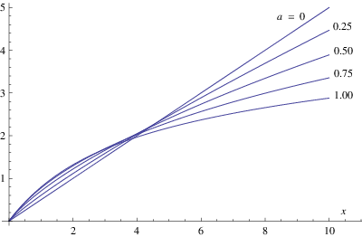
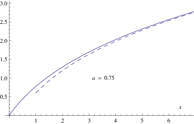
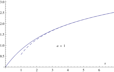
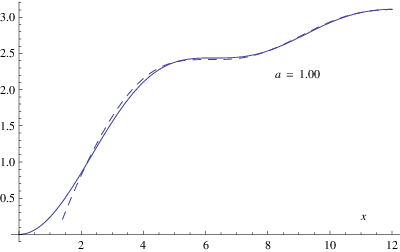
In Fig. 1 we show some plots of Einα,1​(x)\hbox{Ein}_{\alpha,1}(x) for values of α\alpha in the range 0<α≤10<\alpha\leq 1. In Fig. 2 the asymptotic approximations for two values of α\alpha are shown compared with the corresponding curves of Einα,1​(x)\hbox{Ein}_{\alpha,1}(x).

Table 1: The absolute relative error in the computation of Einα,β​(x)\hbox{Ein}_{\alpha,\beta}(x) from Theorem 2 for different values of α\alpha and xx when β=1\beta=1.
xx α=0.25\alpha=0.25 α=0.40\alpha=0.40 α=0.50\alpha=0.50 α=0.75\alpha=0.75 α=1.00\alpha=1.00
5 1.602​(−04)1.602(-04) 1.678​(−05)1.678(-05) 2.012​(−04)2.012(-04) 2.115​(−04)2.115(-04) 5.249​(−04)5.249(-04)
10 5.733​(−07)5.733(-07) 1.735​(−07)1.735(-07) 4.413​(−07)4.413(-07) 2.339​(−07)2.339(-07) 1.442​(−06)1.442(-06)
20 3.680​(−11)3.680(-11) 3.031​(−11)3.031(-11) 6.526​(−12)6.526(-12) 9.362​(−12)9.362(-12) 2.753​(−11)2.753(-11)
30 1.808​(−16)1.808(-16) 9.384​(−16)9.384(-16) 1.543​(−16)1.543(-16) 1.337​(−16)1.337(-16) 7.595​(−16)7.595(-16)
xx α=1.20\alpha=1.20 α=1.40\alpha=1.40 α=1.60\alpha=1.60 α=1.80\alpha=1.80 α=2.00\alpha=2.00
5 1.121​(−03)1.121(-03) 1.301​(−04)1.301(-04) 5.279​(−03)5.279(-03) 1.407​(−02)1.407(-02) 1.550​(−03)1.550(-03)
10 4.345​(−06)4.345(-06) 3.168​(−05)3.168(-05) 2.103​(−04)2.103(-04) 1.536​(−04)1.536(-04) 2.849​(−06)2.849(-06)
20 2.147​(−10)2.147(-10) 2.277​(−08)2.277(-08) 1.671​(−06)1.671(-06) 4.751​(−05)4.751(-05) 4.926​(−10)4.926(-10)
30 4.388​(−14)4.388(-14) 2.363​(−11)2.363(-11) 2.125​(−08)2.125(-08) 6.216​(−06)6.216(-06) 1.613​(−14)1.613(-14)

(aa)Refer to caption

Figure 1: Plots of Einα,1​(x)\hbox{Ein}_{\alpha,1}(x) for different values of α\alpha.

(aa)Refer to caption   (bb)Refer to caption

Figure 2: Plots of Einα,1​(x)\hbox{Ein}_{\alpha,1}(x) (solid curves) and the leading asymptotic approximation (dashed curves) for (aa) α=0.75\alpha=0.75 and (bb) α=1\alpha=1

Table 2 shows the values of the absolute relative error in the computation of Einα,β​(z)\hbox{Ein}_{\alpha,\beta}(z) from the asymptotic expansions in Theorem 1 for complex zz for values of α\alpha in the range 0<α≤20<\alpha\leq 2. It will noticed that there is a sudden reduction in the error when α=1\alpha=1 and θ=π/4\theta=\pi/4. In this case, the value of θ0=12​π\theta_{0}=\hbox{${\textstyle\frac{1}{2}}$}\pi and a more accurate treatment would include the exponentially small contribution z​ℰα,β​(z)z{\cal E}_{\alpha,\beta}(z). When this term is included we find the absolute relative error equal to 6.935×10−116.935\times 10^{-11}.

Table 2: The absolute relative error in the computation of Einα,β​(z)\hbox{Ein}_{\alpha,\beta}(z) from Theorem 1 for different α\alpha and θ\theta when z=20​ei​θz=20e^{i\theta} and β=1/3\beta=1/3.
θ\theta α=0.40\alpha=0.40 α=0.50\alpha=0.50 α=1.00\alpha=1.00 α=1.50\alpha=1.50 α=2.00\alpha=2.00
0 2.400​(−08)2.400(-08) 5.494​(−10)5.494(-10) 2.702​(−10)2.702(-10) 1.572​(−06)1.572(-06) 5.119​(−10)5.119(-10)
π/4\pi/4 2.553​(−08)2.553(-08) 1.820​(−09)1.820(-09) 1.142​(−07)1.142(-07) 1.202​(−08)1.202(-08) 8.204​(−08)8.204(-08)
π/2\pi/2 3.026​(−08)3.026(-08) 4.057​(−09)4.057(-09) 1.756​(−10)1.756(-10) 2.021​(−08)2.021(-08) 3.684​(−07)3.684(-07)
3​π/43\pi/4 3.897​(−08)3.897(-08) 8.028​(−09)8.028(-09) 1.423​(−09)1.423(-09) 2.320​(−07)2.320(-07) 8.204​(−08)8.204(-08)
π\pi 5.398​(−08)5.398(-08) 1.617​(−08)1.617(-08) 6.457​(−09)6.457(-09) 3.005​(−03)3.005(-03) 5.119​(−10)5.119(-10)

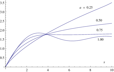
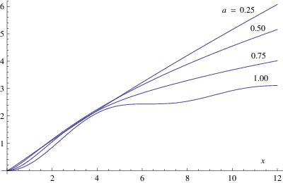
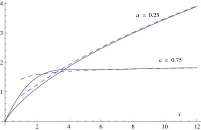
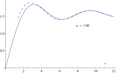
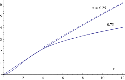
Finally, in Table 3 we present the error associated with the expansions of the generalised sine and cosine integrals Sinα,β​(x)\hbox{Sin}_{\alpha,\beta}(x) and Cinα,β​(x)\hbox{Cin}_{\alpha,\beta}(x) as x→+∞x\to+\infty given in Theorems 3–5. For Sinα,β​(x)\hbox{Sin}_{\alpha,\beta}(x), the logarithmic expansion in (4.4) arises for α=14\alpha=\hbox{${\textstyle\frac{1}{4}}$} and α=12\alpha=\hbox{${\textstyle\frac{1}{2}}$}; for Cinα,β​(x)\hbox{Cin}_{\alpha,\beta}(x) the logarithmic expansion in (4.5) arises for α=13\alpha=\hbox{${\textstyle\frac{1}{3}}$}. In Fig. 3 are shown plots33 3 We remark that the plot of Cinα​1​(x)\hbox{Cin}_{\alpha 1}(x) in Fig. 3(b) differs from that shown in Fig. 4 of [2]. of Sinα,1​(x)\hbox{Sin}_{\alpha,1}(x) and Cinα,1​(x)\hbox{Cin}_{\alpha,1}(x) for different α\alpha and in Fig. 4 the leading asymptotic approximations from the expansions in Theorem 5 are compared with the corresponding plots of these functions.

Table 3: The absolute relative error in the computation of Sinα,β​(x)\hbox{Sin}_{\alpha,\beta}(x) and Cinα,β​(x)\hbox{Cin}_{\alpha,\beta}(x) from Theorems 3–6 for different α\alpha and xx when β=4/3\beta=4/3 .
Sinα,β​(x)\hbox{Sin}_{\alpha,\beta}(x)
xx α=1/4\alpha=1/4 α=1/3\alpha=1/3 α=1/2\alpha=1/2 α=2/3\alpha=2/3 α=1\alpha=1
10 4.396​(−07)4.396(-07) 1.394​(−08)1.394(-08) 1.785​(−06)1.785(-06) 3.410​(−06)3.410(-06) 1.012​(−05)1.012(-05)
20 3.213​(−11)3.213(-11) 1.171​(−13)1.171(-13) 3.920​(−11)3.920(-11) 2.076​(−08)2.076(-08) 3.094​(−11)3.094(-11)
25 2.373​(−13)2.373(-13) 3.792​(−14)3.792(-14) 2.098​(−13)2.098(-13) 4.437​(−10)4.437(-10) 3.270​(−12)3.270(-12)
30 1.879​(−15)1.879(-15) 5.065​(−15)5.065(-15) 1.172​(−15)1.172(-15) 8.197​(−12)8.197(-12) 8.010​(−15)8.010(-15)
Cinα,β​(x)\hbox{Cin}_{\alpha,\beta}(x)
xx α=1/4\alpha=1/4 α=1/3\alpha=1/3 α=1/2\alpha=1/2 α=2/3\alpha=2/3 α=1\alpha=1
10 9.237​(−08)9.237(-08) 3.787​(−07)3.787(-07) 6.608​(−07)6.608(-07) 2.270​(−05)2.270(-05) 7.756​(−06)7.756(-06)
20 1.293​(−12)1.293(-12) 4.473​(−12)4.473(-12) 1.090​(−11)1.090(-11) 2.462​(−10)2.462(-10) 2.576​(−10)2.576(-10)
25 8.066​(−14)8.066(-14) 2.334​(−16)2.334(-16) 5.326​(−14)5.326(-14) 6.881​(−11)6.881(-11) 1.437​(−12)1.437(-12)
30 1.160​(−16)1.160(-16) 9.285​(−17)9.285(-17) 2.764​(−16)2.764(-16) 2.934​(−12)2.934(-12) 7.716​(−15)7.716(-15)

(aa)Refer to caption   (bb)Refer to caption

Figure 3: Plots of the generalised sine and cosine integrals (aa) Sinα,1​(x)\hbox{Sin}_{\alpha,1}(x) and (bb) Cinα,1​(x)\hbox{Cin}_{\alpha,1}(x) for α=0.25,0.50,0.75,1\alpha=0.25,0.50,0.75,1.

(aa)Refer to caption   (bb)Refer to caption

(cc)Refer to caption  (dd)Refer to caption

Figure 4: Plots of the generalised sine and cosine integrals (solid curves) and their leading asymptotic approximations (dashed curves) from Theorems 3, 4 and 5: (aa) Sinα,1​(x)\hbox{Sin}_{\alpha,1}(x) when α=0.25,0.75\alpha=0.25,0.75, (bb) Sinα,1​(x)\hbox{Sin}_{\alpha,1}(x) when α=1\alpha=1, (cc) Cinα,1​(x)\hbox{Cin}_{\alpha,1}(x) when α=0.25,0.75\alpha=0.25,0.75 and (dd) Cinα,1​(x)\hbox{Cin}_{\alpha,1}(x) when α=1\alpha=1.

References

  • [1] W.B. Ford, The Asymptotic Developments of Functions defined by Maclaurin Series, University of Michigan Studies, Scientific Series, Vol. 11, 1936.
  • [2] F. Mainardi and E. Masina, On modifications of the exponential integral with the Mittag-Leffler function. Fract. Calc. Appl. Anal. 21 (2018) 1156–1169.
  • [3] F. Mainardi, E. Masina and G. Spada, A generalization of the Becker model in linear viscoelasticity: Creep, relaxation and internal friction. Mechanics of Time-Dependent Materials, Publ. online 2 Feb. 2018. pp. 12 [arXiv:1707.05188].
  • [4] F.W.J. Olver, D.W. Lozier, R.F. Boisvert and C.W. Clark (eds.), NIST Handbook of Mathematical Functions, Cambridge University Press, Cambridge, 2010.
  • [5] R.B. Paris, Exponentially small expansions of the confluent hypergeometric functions, Appl. Math. Sci. 7 (2013) 6601–6609.
  • [6] R.B. Paris, Asymptotics of the special functions of fractional calculus, in Handbook of Fractional Calculus with Applications, Vol.1, (eds. A. Kochubei and Y. Luchko), pp. 297–325, De Gruyter, Berlin, 2019.
  • [7] R.B. Paris and D. Kaminski, Asymptotics and Mellin-Barnes Integrals, Cambridge University Press, Cambridge 2001.
  • [8] Wolfram Research, Inc., Mathematica, Version 7, Champaign, Illinois (2008).