Top-Down Shape Abstraction Based on Greedy Pole Selection
Abstract
Motivated by the fact that the medial axis transform is able to encode the shape completely, we propose to use as few medial balls as possible to approximate the original enclosed volume by the boundary surface. We progressively select new medial balls, in a top-down style, to enlarge the region spanned by the existing medial balls. The key spirit of the selection strategy is to encourage large medial balls while imposing given geometric constraints. We further propose a speedup technique based on a provable observation that the intersection of medial balls implies the adjacency of power cells (in the sense of the power crust).
We further elaborate the selection rules in combination with two closely related applications. One application is to develop an easy-to-use ball-stick modeling system that helps non-professional users to quickly build a shape with only balls and wires, but any penetration between two medial balls must be suppressed. The other application is to generate porous structures with convex, compact (with a high isoperimetric quotient) and shape-aware pores where two adjacent spherical pores may have penetration as long as the mechanical rigidity can be well preserved.
Index Terms:
Shape abstraction, medial surface, power crust, porous structure, ball-stick toy, power diagram.I Introduction
Shape abstraction draws much attention in computer vision and pattern recognition since it is closely related to shape recognition and shape understanding. One of the key motivations of shape abstraction is parsimony of description, i.e., an object could be described by relatively few primitives, each of which in turn requiring only a few parameters [1]. It is a hard yet fascinating problem [2].
Different from explaining objects with volumetric primitives based on learning techniques [1], in this paper, we study the problem of approximating the original enclosed volume using as few medial balls as possible motivated by the fact that the medial axis transform is able to encode nearly the complete shape, which approaches this problem motivated by the geometry.
It’s well known that the full set of medial balls defines the enclosed volume , and thus we intend to use a subset of representative medial balls to generate the shape abstraction of . In the discrete setting, the medial surface can be approximated by the Voronoi diagram w.r.t. a set of samples extracted from the boundary surface, while the medial balls can be replaced by polar balls centered at a subset of Voronoi vertices (also named as poles) [3, 4, 5]. We propose to progressively select new polar balls, in a top-down style, to enlarge the region occupied by the existing polar balls. The key point of selecting poles is to encourage large polar balls subject to given geometric constraints.
In implementation, we require an efficient proximity query technique to determine how a given polar ball intersects with a set of existing polar balls. Interestingly, we observe that there is a provably effective speedup technique that the intersection of polar balls implies the adjacency of power cells (in the sense of the power crust [4, 5, 6, 7, 8, 9]). Therefore, we maintain a dynamic power diagram w.r.t. a set of poles to support efficient proximity query rather than detect the intersection between polar balls in a brute-force manner. We further put forward two closely related applications including ball-stick modeling and porous structure generation.
Our contributions are three-fold:
- 1.
We propose a greedy selection strategy that approximates the enclosed volume with as few as possible polar balls.
- 2.
- 3.
We elaborate the selection rules in combination with two closely related applications and validate the uses and effectiveness of our algorithm, See Figure 1.

II Related Work
Medial surface. The medial axis transform (MAT), as a complete shape descriptor [10], is central to various applications such as shape recognition/manipulation and surface approximation [11]. Given a closed, oriented and bounded 2-manifold surface in , a ball inside the volume enclosed by is said to be maximal if no other ball in contains . In fact, the medial surface is formed by the locii of the centers of maximal balls inside . Furthermore, the union of maximal balls defines .
Generally the MAT problem doesn’t have a closed-form solution, and one has to seek for a numerical solution instead. The most popular technique is to initialize the medial surface using the Voronoi diagrams w.r.t. a set of sufficiently dense boundary samples and then prune spikes or optimize mesh tessellations based on various rules. There are many existing approaches on this side, such as -medial axis [12], quadratic error metric (QEM) based MAT [13], delta medial axis (DMA) [14], bending potential ratio (BPR) pruning [15], erosion thickness (ET) measure [16] and voxelization based pruning [17]. The simplified MAT, without doubt, cannot exactly recover the original boundary surface, and thus one has to control the error metric by computing the Hausdorff distance [18] or adaptively classifying geometric features [6].
The power crust [4, 5, 6, 7, 8, 9] also begins with Voronoi diagrams w.r.t. boundary samples, but uses a subset of Voronoi vertices as poles to generate MAT approximation by computing a power diagram w.r.t. poles. In fact, it builds an inverse transform from the MAT to the surface representation, and thus facilitates many applications such as surface reconstruction and surface offsetting. The theme of this paper, i.e. greedily selecting some poles for shape abstraction, is closely related to the power crust theory. We shall give the theoretical foundation in the next section.
Shape abstraction. Shape abstraction is an important research topic in computer vision and pattern recognition and central to shape recognition and shape understanding [1]. On some occasions it is also called shape averaging or shape simplification. Abstract shape representations may vary with different contexts. Curves [19], contours [20, 19], skeletons [21] and even black-and-white images [22] are all commonly used abstract shape representation forms. There is a large body of literature on how to approximate the given surface/volume using a set of shape primitives that include planar faces [23, 24], cylinders, spheres [25], tori [26], or even superquadrics [27], hyperquadrics [28] and blobby models [29]. An important application of shape abstraction is to help understand the 3D structure/layout of a given scene, as well as the spatial, functional, and semantic relationships between objects in the scene [30, 31]. Beside the above mentioned geometry based approaches, Gestalt principles can also serve as a guide to shape simplification and abstraction [32, 33], especially useful for automatically simplifying line drawings of architectural buildings [34, 35].
In this paper, we select as few medial balls as possible to approximate the original enclosed volume by the boundary surface, which is from a geometric perspective, rather than based on learning techniques [1]. We define a priority measure to encourage large medial balls while suppressing serious penetration between medial balls.
Easy modeling. Simple modeling tools are becoming popular nowadays - nonprofessional users can build their own favorite toys/products with a 3D printer. For example, Igarashi et al. [36] proposed an interactive system that supports constructing a 3D polygonal surface from the 2D silhouette. Mori et al. [37] introduced the physical simulation technique to help design original plush toys. They also introduced simple physical simulation to improve digital fabrication. Nealen et al. [38] proposed to design freeform surfaces with a collection of 3D curves. Users can not only use strokes as handles to control the geometry, but also add, remove, and deform these control curves easily. Igarashi et al. [39] introduced an interactive system named “Beady” to assist the design and construction of customized 3D beadwork. Attene et al. [40] proposed to approximate a 3D model with a set of planes, spheres and cylinders based on hierarchical face clustering, but they allow intersection between shape primitives. Besides, various easy modeling approaches are applied in education, art production, products design, and pattern recognition. Generally speaking, the convenience of easy modeling comes from at least two aspects: (1) an image, or a point cloud, or a 3D digital model as the hint and (2) intelligent/fast computation to facilitate real-time user interaction.
In fact, easy modeling with a set of penetration-free shape primitives of prescribed types is our main interest. One of our applications in this paper is to develop an easy-to-use ball-stick modeling system that helps children to quickly build a shape with only balls and wires. The key lies in how to approximately represent the enclosed volume by a set of penetration-free medial balls with various sizes (typically customized in advance).
Porous structure. Porous structures are ubiquitous in nature and widely used in our daily life because of nice physical properties. For example, porous solids have been proved to be good candidates as the carbon dioxide recycling sorbents [41, 42]. Porous structure design has drawn much attention in recent years especially with the innovation of the additive manufacturing technology. An important research topic is to reduce the material cost, as well as the weight, of a given object while providing a durable printed model that is resistant to impact and external forces [43]. Wang et al. [44] discussed cost-effective 3D printing by reinforcing a thin shell with skin-frame structures. Lu et al. [43] proposed a hollowing optimization algorithm based on the concept of honeycomb structure. Recently, Mao et al. [45] used hybrid structures for designing the support structure.
In fact, finite element analysis of stress is central to fabrication oriented design. For example, Stava et al. [46] suggested strengthening printed objects by hollowing, local thickening, and adding extra struts. There is a trend of addressing these issues based on topology optimization [47, 48, 49, 50]. Wu et al. [51] proposed a method to generate application-specific infill structures on rhombic cells so that the resultant structures can automatically satisfy manufacturing requirements on overhang-angle and wall-thickness. Groen et al. [52] introduced an efficient homogenization based approach to perform topology optimization of coated structures with orthotropic infill material. We refer to [47] for a survey.
Inspired by the structure of the spherical inverse opal, we notice that the convexity and compactness (high isoperimetric quotient) of pores are central to preserving mechanical rigidity. Therefore, in this paper, we proposed to use medial balls as primitives to generate pores but allow moderate penetration between neighboring pores (we add an additional partition board to separate neighboring pores). In implementation, our algorithm is based on a greedy selection strategy that gives a higher priority to those large medial balls but suppresses serious penetration between medial balls.
III Theoretical Background
III-A Voronoi diagram & power diagram

Voronoi diagramPower diagram
Voronoi diagrams are used to partition a given domain into regions based on the straight-line distance to a set of generators such that dominates the subregion (also called a cell):
| (1) |
Power diagrams can be viewed as an extension of Voronoi diagrams, where each generator is equipped with a weight to adjust the influence range. That is to say, by assuming the power distance between and the weighted generator to be , the cell dominated by becomes
| (2) |
A generator with a larger weight is more dominant, and when all the weights are equal, the power diagram reduces to a Voronoi diagram. Different from the Voronoi diagram, there may be some generators hidden from the power diagram, which means these generators have no corresponding dominant regions. In Figure 2, we show a Voronoi diagram and a power diagram respectively.
III-B Medial surface
![[Uncaptioned image]](1910.08954v3/MA_2d.png)
Suppose that is a closed, oriented and bounded 2-manifold surface in . By the term medial surface, we mean the loci given by the center of a moveable sphere inside that has at least two touching points with . The medial surface of , combined with the medial radius function , is called medial-axis transform (MAT), denoted by a pair .
III-C Feature-preserving sampling
Definition III.1.
Given a surface and a point , the local feature size (LFS) of , denoted by , is defined to be the distance between and the medial surface .
Definition III.2.
Let be a set of samples extracted from . If , there exists a sample such that , then is an -dense sample set. If , there exists a sample such that , then is an -LFS sample set.
III-D Inside/outside poles
![[Uncaptioned image]](1910.08954v3/poles.png)
In the discrete setting, the Voronoi diagrams w.r.t. a set of sufficiently dense boundary samples in are commonly used to initialize the medial surface. Given an -LFS sample set, each sample dominates a cell across (generally a sufficiently large box is used to make ’s cell to be closed). On either side of the surface, there is a cell vertex farthest from , respectively named an inside pole and an outside pole; See the inset figure. Each pole defines a polar ball , where is the sample point closest to .
Definition III.3.
The power crust is the boundary between the power diagram cells belonging to inside poles and power diagram cells belonging to outside poles.
The power crust is able to approximate the original boundary surface under the condition that the samples are sufficiently dense [5].
Lemma III.1.
Let and be respectively the inside and outside poles w.r.t. an -LFS sample set. When approaches 0, the power crust given by and approximates the surface .
It can be shown that the following observation naturally holds based on Lemma III.1. (More theoretical results are available in [5, 53, 54], and we organize them in Appendix A.)
Corollary III.1.1.
Let be the inside pole set w.r.t. an -LFS sample set. When approaches 0, the union of the polar balls
approximates the volume enclosed by .
Due to the approximation ability of polar balls, we make no distinction between polar balls and medial balls in later sections.
III-E Proximity query between polar balls
Corollary III.1.1 motivates us to use a subset of representative inside poles , or alternatively their corresponding polar balls , to generate the shape abstraction of the whole enclosed volume. For this purpose, we adopt a top-down pole selection strategy that encourages large polar balls while suppressing serious intersection between polar balls.
In implementation, we require an efficient proximity query technique to determine how a given polar ball intersects with a set of existing polar balls. In fact, there is a fundamental relationship between the proximity of polar balls and the proximity of power cells.
Lemma III.2.
Suppose that and are two balls in . If intersects the ball at a disk, for every point in the plane of the disk, has equal weighted distances to and , i.e. where the weight is set to be the squared radius.
In other words, under the condition that the polar ball intersects the ball at a disk, the disk must be coplanar with the equal-power plane w.r.t. and (each pole is equipped with a weight of the squared medial radius). We further observe that the power diagram is able to serve as an effective tool for polar-ball based dynamic proximity query, which is the following theorem.
Theorem III.3.
Let and be respectively the inside poles and the outside poles w.r.t. a sufficiently dense -LFS sample set on the surface . Suppose that we have a subset of inside polar balls centered at . For another inside pole , the statement that the polar ball centered at intersects with one of the existing polar balls implies that there exists such that ’s cell is neighboring to ’s cell in the power diagram w.r.t. .


(a)(b)
Proof.
We consider the power diagram w.r.t. where each pole is weighed by the square of the radius of its polar ball.
Suppose that the pole is defined based on some boundary sample point , which implies that is closer, or at least equally distant, to than any other poles belonging to . It is easy to verify that . Considering that is located outside/on the polar balls given by , the power distance between and any pole in is non-negative. Therefore, ’s cell is not empty (since the cell contains at least ). It can be further concluded that ’s cell is convex.
Now we assume that ’s cell is not neighboring to any cell given by , which implies that the boundary of ’s cell is formed by and the poles in . On one hand, we can see that for any point on the boundary of ’s cell (since has equal power distances to and some outside pole in ; but the power distance between and any outside pole in is non-negative), which implies that the polar ball centered at is totally inside ’s cell (note that for any point on the surface of the polar ball centered at ); See Figure 3(a). On the other hand, the equal-power plane between and any pole in cannot pass through ’s cell since doesn’t contribute to the boundary of ’s cell at all.
According to the given condition that ’s polar ball intersects with one of the polar balls given by , without loss of generality, we assume that ’s polar ball intersects with ’s polar ball, where . The two polar balls intersects at a disk and any point in this disk is located inside ’s polar ball and thus also inside ’s cell. However, the disk is coplanar with the equal-power plane between and , which shows that this equal-power plane is given by and a pole in but passes through ’s cell (see Figure 3(b)), which contradicts to the above assumption. ∎
Corollary III.3.1.
Let and be respectively the inside poles and the outside poles w.r.t. a sufficiently dense -LFS sample set on the surface . Suppose that we have two inside polar ball sets centered at with . The statement that ’s polar balls intersect with ’s polar balls implies that there exists two inside poles and such that ’s cell is neighboring to ’s cell in the power diagram w.r.t. .
IV Problem formulation
Suppose that we have obtained a full set of inside poles, i.e. , which define a set of medial-axis balls inside the volume enclosed by the surface . Our task is to develop a strategy on how to incrementally select some representative poles, generally just a few, to approximate the volume as far as possible under some specified geometric constraints.
In particular, we shall discuss the pole selection in detail in combination with two separate applications: (1) ball-stick toy design where we need to use a set of separate medial balls with various sizes, connected by wires, to convey the abstracted shape, and (2) porous structure generation where two spherical pores may have penetration but every pore must have a compact shape (with a high isoperimetric quotient). See Section V and Section VI respectively.
V Ball-Stick Toy Building

We first discuss the shape approximation application in ball-stick toy building. Many experts in teaching children found that modeling various shapes with some basic components, e.g., clay or magnetic sheets, have a very positive influence on intelligence development and can make children become more creative. Ball-stick toy design (see Figure 4), i.e. assembling balls and sticks (or wires) into a target shape, is one of the most popular educational games. We find that the technical principles behind the ball-stick toy design have a close relationship to the theme of this paper, i.e. medial ball based shape abstraction.
V-A Selection strategy

Let be the full set of inside poles. Technically speaking, we have to select a subset of polar balls, generally not many, centered at a pole set such that the union of balls roughly represents the enclosed volume of the input shape. Note that any penetration is not allowed between selected polar balls.
Initially, is an empty set. We have to select the largest polar ball and add the corresponding pole into . After that, we enlarge the set by repeatedly selecting a new inside pole . A natural idea is to use the following greedy strategy to incrementally enlarge until the selected medial balls, after connected, sufficiently resemble the entire shape; See Figure 5 for illustration.
| (3) |
We denote , and then Eq. (3) can be rewritten as
| (4) |
It’s easy to verify the following observation.
Theorem V.1.
Eq. (4) reports a non-increasing medial-radius sequence.
Based on Theorem V.1, we can stop the selection process until the medial radius is less than a prescribed tolerance . The pseudo-code of a naïve implementation is described in Algorithm 1.
repeat 2
for every pole in do 3
end for 4
end if 6
Algorithm 1 is not efficient because we have to check the intersection, one by one, between ’s medial ball and the existing medial balls given by . We shall discuss the speedup strategy int the following subsection.
V-B Algorithm speedup
Recall that during each iteration of Algorithm 1, we have to test if the top-priority pole popped from the priority queue is able to define a medial ball that doesn’t have penetration with those medial balls given by . The key of speeding up Algorithm 1 lies in how to quickly report those candidate poles in that are “sufficiently close” to such that penetration between medial balls may occur, rather than in a brute-force manner.
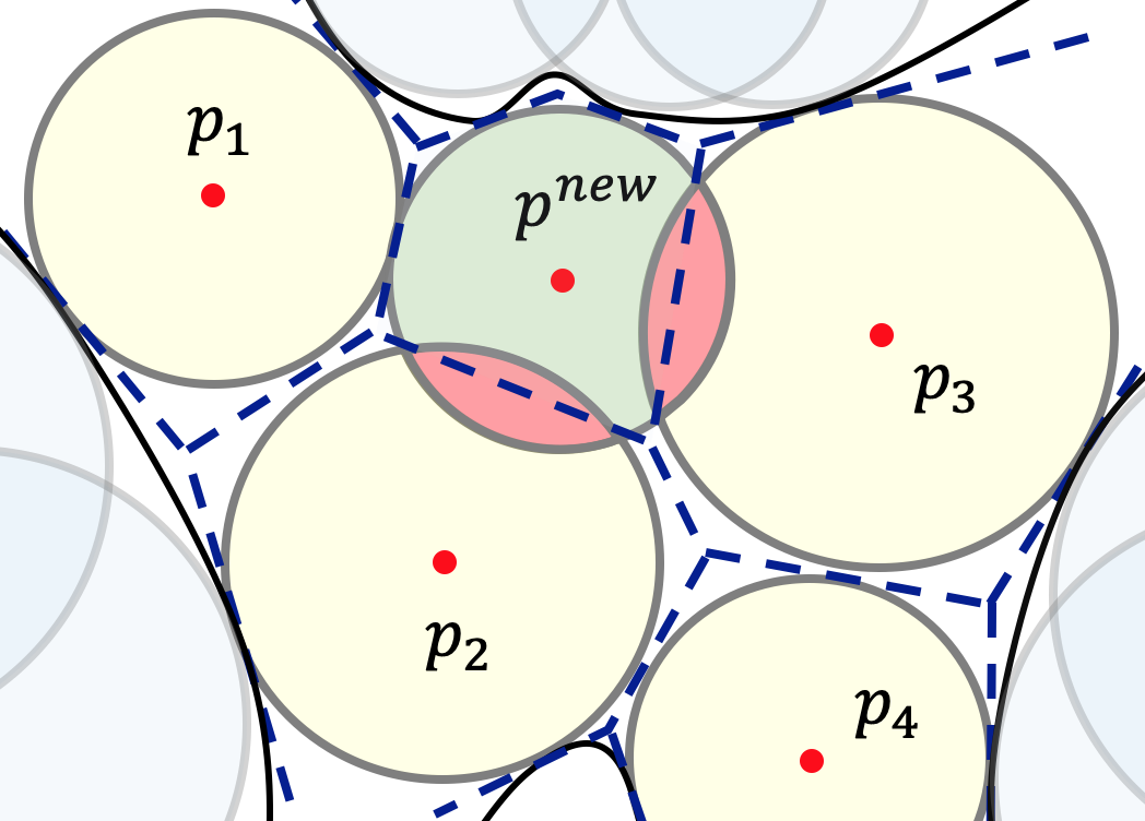
Theorem III.3 states that the intersection between medial balls implies the adjacency between power cells. Suppose that we maintain a dynamic power diagram throughout the algorithm. Now we update the power diagram to ( is the set of outside poles), which requires only a little cost due to the incremental change of partition configuration. As Figure 6 shows, the medial balls colored in yellow are defined by while the medial ball colored in green is given by that has a medial radius . We can see that ’s cell is neighboring to 3 existing poles, i.e. in . Theorem III.3 tells us ’s medial ball cannot intersect with those medial balls given by Therefore, it suffices to check the assertions one by one. If all the assertions are true, we accept as the next candidate and add it into ; Otherwise, we consider the next top-priority pole popped from the priority queue. Detailed performance contrast between the brute-force method and the accelerated version will be given in Section V-E.
V-C Connection between poles


We have to connect the balls with wires to consolidate the structure of the toy. Recall that each surface sampling point dominates a separate Voronoi cell restricted in the volume, and the union of the restricted Voronoi cells is said to be restricted Voronoi diagram (RVD). The RVD naturally induces a graph whose vertex set comprises the selected poles. The key idea of bridging the selected poles is to find a Steiner tree belonging to by taking each selected pole as a terminal. For this purpose, we have to define a weighting scheme such that the tree with the highest centredness can be found. In this paper, we define the weight of a pair of adjacent MA points as follows:
| (5) |
The parameter serves as a penalty to balance the two terms. The term is to select a path along which the medial radius changes slowly, the denominator is to keep the path away from the boundary surface, and the term is to select an as-short-as-possible path. After is fixed, we take the Steiner tree [55] of the graph as the final connection structure between poles, where the selected poles are taken as terminals; See Figure 7.
In fact, a Steiner tree is cycle free and thus can only be used to represent the skeleton of a genus-0 model. For a high-genus model, however, the skeleton is not a tree any more. We need to detect topology-aware loops first [56], and then with all the poles in , together with the topologically characteristic loops, as terminals, we compute a connection structure that is structurally conformal to the boundary shape. Details are available in Appendix B.
V-D Feature preserving

Generally speaking, it is hard to use a sequence of balls to approximate the sharp features that are important hints to understand shapes. To enable the ball-stick toy resemble the original input model as far as possible, we propose two strategies in the following.
Separation gaps. In Eq. (4), is a hard constraint to guarantee the separation between medial balls. In fact, we can further force the selected medial balls to be separated in a prescribed gap to facilitate the placement of wires.
| (6) |
A side effect is to push the medial balls to around the sharp features. In spite of the difference between Eq. (4) and Eq. (6), the speedup technique mentioned in Section V-B still works with only a slight modification (we just change the medial radius of temporarily from to before updating ).
Feature points. We further suggest adding significant feature points into the RVD-induced graph . Suppose that is located on the surface of the Voronoi cell of a certain sample point . We connect to any Voronoi vertex of ’s cell. In this way, we augment to . Similarly, we take the Steiner tree of to generate the final connection structure between selected poles and feature points; See Figure 8 for illustration.
V-E Evaluation

We implemented and experimented with our algorithm on a computer with a 64-bit version of macOS Mojave system, a 2.7 GHz Intel(R) Core(TM) i5 CPU and 16 GB memory. The coding language is C++. We employ the adaptive blue noise sampling approach [57] in the sampling step. For simplicity, we remesh the Teddy model, the Baby-Camel model and the Gorilla model into 60K triangles and set the number of samples to be 4K. Besides, the program terminates when the radius of the top-priority ball popped from the priority queue is less than of the bounding box size. The parameter in Eq. (6) is set to be of the bounding box size while the parameter in Eq. (5) is set to 3.
Our algorithm consists of four main operations. We use T1, T2, T3, T4 to respectively denote the four time costs:
- T1:
Compute Voronoi diagram w.r.t. boundary samples;
- T2:
Label inside and outside poles;
- T3:
Extract RVD w.r.t. boundary samples;
- T4:
Connect poles in .
The timing statistics (in seconds) for the models shown in Figure 7,8,9 are available in Table I, where the # Vertice denotes the number of boundary samples. In particular, we define 4 customized ball sizes, respectively 1.5cm, 2cm, 4.5cm, 5.5cm in diameter. Users can not only build their favorite ball-stick toys by reference to our generated results (see Figure 9), but also transform it into various poses (see the teaser figure).
| Models | Running Time (s) | ||||
|---|---|---|---|---|---|
| Name | V | T1 | T2 | T3 | T4 |
| Ostrich (2D) | 500 | 0.004 | 0.007 | 0.002 | 0.139 |
| Dinosaur (2D) | 500 | 0.005 | 0.007 | 0.003 | 0.127 |
| Teddy | 4000 | 6.12 | 3.34 | 1.72 | 0.42 |
| Baby Camel | 4000 | 6.19 | 2.86 | 2.99 | 0.525 |
| Kitten | 4000 | 6.33 | 3.25 | 0.98 | 0.24 |
| Gorilla | 4000 | 5.74 | 3.51 | 1.02 | 0.39 |

In the following, we use Figure 10 to show the performance contrast between the brute-force ball penetration detection strategy (Algorithm 1) and the accelerated strategy (Section V-B). The test is conducted on the Kitten model with 4K points being sampled.
Without doubt, when just a few poles are selected, the brute-force ball penetration detection strategy may be faster. But with the increasing of the number of selected poles, the accelerated strategy outperforms the naiv̈e one. As shown in Figure 10, when the number of selected poles exceeds , our accelerated method exhibits a conspicuous advantage.


(a) (b) (c) (d) (e)
VI Porous Structure Generation
![[Uncaptioned image]](1910.08954v3/SEM-images-of-the-nanocrystalline-Si-inverse-opal-structure-36.png)
In the following, we shall discuss the other application, i.e., how to generate porous structures. Porous structures are ubiquitous in nature due to their nice physical properties. Porous structure design is a fascinating yet challenging research topic in recent years, especially with the innovation of the additive manufacturing technology. As the inset figure shows, the spherical inverse opal is the most common processed and studied self-assembly structure [58]. Compared with other pore structures such as ellipsoids, plates and rods, the spherical inverse opal has better structural mechanical behavior. This motivates us to generate shape-aware spherical porous structures.
VI-A Requirements
We intend to select a set of medial balls to generate porous structures. Before we figure out detailed selection strategies, we made the following two experiments to make clear (1) whether spherical pores are better than pores of other types, and (2) to what degree the penetration between pores reduces the entire mechanical rigidity.

333 333 spherical pores ellipsoidal pores
As Figure 12 shows, we generate a spherical-pore structure and an ellipsoidal-pore structure respectively for the input cube model, and the pores in both configurations are of the same volume size. From the stress nephograms in ABAQUS, we can clearly see that spherical pores are able to better preserve the original mechanical rigidity, which is in line with our initial guess. Therefore we intend to select some representative medial-axis balls as basic primitives to compose the final pore structure.

(a) (b) (c)
Different from the ball-stick toy design, penetration between two medial balls should be allowed as long as the convexity/compactness of each pore is not seriously destroyed. In Figure 13, we show three configurations of pores, i.e. no penetration, moderate penetration and serious penetration. The stress nephograms show that the pore configuration shown in Figure 13(b) saves more material but can well preserve the entire mechanical rigidity. Therefore, we allow moderate intersection between medial balls, rather than enforce a hard constraint of being penetration-free.
VI-B Selection strategy
Based on the above experiments, we consider the selection strategy from two aspects. On one hand, we intend to encourage those large medial balls to be selected into , and on the other hand, we have to enforce a penalty on serious penetration, i.e.,
| (7) |
where is used to balance the two considerations. Similarly, we stop the selection process if the medial radius of is sufficiently small.
If is small, then there may be many thin pores generated due to lack of penalty on penetration; See Figure 11.
If , the to-be-selected pole must be located outside the existing balls. W.l.o.g, we take each surface sample point as a pole whose medial radius is 0. Obviously, all the sample points are located outside the existing medial balls. Therefore, it is easy to infer that
for any boundary sample point. This implies that under the selection criterion
the to-be-selected pole must meet or at least So must be located outside the existing balls. In our experiments, we set without any specification.
VI-C Implementation
In the following, we give a couple of key technical details of algorithm implementation.
Throughout the algorithm, we need to maintain two data structures. One is the priority queue where a pole has a priority of , and the other is a dynamic power diagram w.r.t. .
Imagine that is the newly selected pole that is ready to be added to . According to Eq. (7), the selection of possibly changes the priority of those poles in that are very close to (i.e., penetration occurs between ’s medial ball and ’s medial ball). We need to quickly identify these poles and update their priorities.
Once again, we employ Theorem III.3 to achieve this purpose. Let be the power diagram at this moment, where is the outside pole set. Let be a copy of . We repeatedly label and then remove a pole as long as ’s cell is neighboring to ’s cell in the up-to-date power diagram. We stop the process until ’s cell becomes isolated from those remaining poles in (i.e. the boundary of ’s cell is given by and the outside poles). So far, we have identified a set of poles in whose medial balls possibly intersect with ’s medial ball. We then update the priority of these identified poles. Finally we compute based on a light-weight update of and continue the next iteration.

We need to keep the pores away from the boundary surface in a proper gap. At the same time, a planar separator between neighboring pores is used to preserve rigidity. We introduce a parameter to achieve this purpose.
First, we filter out those inside poles whose medial radius is less than . We then reduce the medial radii of other inside poles by . In fact, the pore belonging to can be obtained by subtracting the medial ball by a sequence of equal-power planes, each of which is given by and a neighboring site (here “neighboring” means that penetration occurs between ’s medial ball and ’s medial ball). In order to guarantee the separator being of a -thickness, we move each equal-power plane in a distance of toward both sides upon penetration between medial balls occurs.
VI-D Evaluation
Our algorithm involves three main operations and we use T1, T2, T3 to respectively represent their time costs. T1: the time cost for computing Voronoi Diagram w.r.t. boundary samples; T2: the time cost for labeling inside and outside poles; T3: the time cost for computing the power diagram w.r.t. . We use totally five models for test; See section views of spherical-pore structures in Figure 14. From the timing statistics in Table II we can see that our algorithm runs in only tens of seconds for 4K samples. Note that generally T3 is related to the number of poles in , which accounts for why T3 is larger for the Fertility model than other models.
| Models | Running Time (s) | Weight Sav- ing Ratio | |||
| Name | V | T1 | T2 | T3 | |
| Kitten | 4000 | 5.91 | 2.11 | 6.62 | 62.85% |
| Fertility | 4000 | 6.09 | 3.23 | 20.67 | 57.71% |
| Horse | 4000 | 6.29 | 2.82 | 7.79 | 51.86% |
| Bunny | 4000 | 5.44 | 3.09 | 4.65 | 54.82% |
| Armodillo | 4000 | 5.95 | 2.65 | 12.43 | 46.95% |
| Item |
|
Honeycomb | ||
| Solid Vol (cm3) | 540.88 | 540.88 | ||
| Actual Material Vol (cm3) | 213.08 | 226.79 | ||
| Max Load (kN) | 0.64 | 0.49 | ||
|
3.00 | 2.16 |

In the following, we discuss how effective our priority update strategy is. Let be a newly selected pole. In fact, a naïve strategy of updating the priorities of the remaining poles is to detect the penetration between and all the poles in . By contrast, our accelerated strategy is to update the priorities of just a few surrounding inside poles, instead of detecting every unselected poles in a brute-force manner. We conducted a test on the Kitten model with 4K samples. The performance statistics are given in Figure 15.
In order to compare with the honeycomb-structure hollowing method [43], we generate two versions of the Kitten model to perform finite element analysis by enforcing a gravity load. The paramter configurations are as follows: Young’s modulus, Poisson’s ratio, mass density are respectively set to 2100, 0.31, 3. The resulting stress nephogram in ABAQUS shows that our spherical-pore Kitten model, in spite of larger weight saving ratio, owns a more uniform distribution of stress. See Figure 16. Note that red means that the stress is high, while blue stands for low stress. It can be seen that the maximum stress of the honeycomb structure occurs around the neck, amounting to 9.736Mpa, which is due to two facts: (a) the honeycomb cells’ surfaces have varying curvatures, and are much different from curvature-uniform spherical pores, and (b) the neck is the weakest part and thus should not be reduced too much in weight.

(a) Spherical pores(b) Honeycomb structure
We used a hydraulic testing machine to report the maximum pressure the model can withstand. We downloaded the honeycomb-structured Trophy model from the project page of [43]. Their theoretical weight saving rate is . For the comparison purpose, we generated a spherical-pore structure with a theoretical weight saving rate of by controlling the number of pores. With PLA+ as the 3D printing material (tensile strength: 60Mpa, bending strength: 87Mpa, bending modulus: 3642Pa), we used an FDM prototyping machine to print the two kinds of porous structures for pressure test. Detailed pressure statistics are available in Table III. Figure 17 captured the moments when the model breaks, and the values of compaction force at the breaking point are 0.64kN (ours) and 0.49kN (honeycomb-structured) respectively. Note that the significant difference in structure is that the honeycomb-structured model was hollowed even around the thin-neck parts, but our algorithm didn’t produce any spherical pores around the neck. Therefore we believe that our proposed algorithm has a big potential in the light-weight product design.

(a) Honeycomb structure(b) Spherical pores
VII Conclusion
In this paper, we studied the medial ball based shape abstraction problem, i.e., how to use as few medial balls as possible to approximate the original enclosed volume while imposing given geometric constraints. Our technical contribution is to propose a top-down selection strategy to encourage large medial balls while taking into account specific requirements. We develop an effective speedup technique based on a provable observation that the intersection of medial balls implies the adjacency of power cells (in the sense of the power crust).
We further explore the uses of our algorithm in combination with two closely related applications. In the ball-stick design application, our algorithm is able to help non-professional users to quickly build a shape with only balls and wires, where any penetration between two medial balls must be suppressed. In the porous structure generation application, however, moderate penetration between two adjacent spherical pores are allowed to maximize the ratio of material saving while preserving structural rigidity. We use both FEA and real physical tests to validate the effectiveness.
Acknowledgments
The authors would like to thank the anonymous reviewers for their valuable comments and suggestions. This work is supported by National Natural Science Foundation of China (61772016, 61772318) and Research Grant Council of Hong Kong (GRF 17263316).
References
- [1] S. Tulsiani, H. Su, L. J. Guibas, A. A. Efros, and J. Malik, “Learning shape abstractions by assembling volumetric primitives,” in CVPR. IEEE Computer Society, 2017, pp. 1466–1474.
- [2] D. L. Borges and R. B. Fisher, “Class-based recognition of 3D objects represented by volumetric primitives,” Image and Vision Computing, vol. 15, no. 8, pp. 655–664, 1997.
- [3] N. Amenta, M. Bern, and M. Kamvysselis, “A new Voronoi-based surface reconstruction algorithm,” in Proceedings of the 25th Annual Conference on Computer Graphics and Interactive Techniques. ACM, 1998, pp. 415–421.
- [4] N. Amenta, S. Choi, and R. K. Kolluri, “The power crust,” in Proceedings of the sixth ACM symposium on Solid modeling and applications. ACM, 2001, pp. 249–266.
- [5] ——, “The power crust, unions of balls, and the medial axis transform,” Computational Geometry, vol. 19, no. 2-3, pp. 127–153, 2001.
- [6] B. Miklos, J. Giesen, and M. Pauly, “Discrete scale axis representations for 3D geometry,” ACM Transactions on Graphics (TOG), vol. 29, no. 4, p. 101, 2010.
- [7] D. Attali and A. Montanvert, “Modeling noise for a better simplification of skeletons,” in International Conference on Image Processing. IEEE, 1996, pp. 13–16.
- [8] T. K. Dey and W. Zhao, “Approximating the medial axis from the Voronoi diagram with a convergence guarantee,” Algorithmica, vol. 38, no. 1, pp. 179–200, 2004.
- [9] J. Giesen, E. A. Ramos, and B. Sadri, “Medial axis approximation and unstable flow complex,” in Proceedings of the twenty-second annual symposium on Computational geometry. ACM, 2006, pp. 327–336.
- [10] H. Blum, “A transformation for extracting new descriptors of shape,” Models for Perception of Speech and Visual Forms, pp. 362–380, 1967.
- [11] E. C. Sherbrooke, N. M. Patrikalakis, and E. Brisson, “Computation of the medial axis transform of 3-d polyhedra,” in Proceedings of the third ACM symposium on Solid modeling and applications. ACM, 1995, pp. 187–200.
- [12] F. Chazal and A. Lieutier, “The “-medial axis”,” Graphical Models, vol. 67, no. 4, pp. 304–331, 2005.
- [13] P. Li, B. Wang, F. Sun, X. Guo, C. Zhang, and W. Wang, “Q-MAT: Computing medial axis transform by quadratic error minimization,” ACM Transactions on Graphics (TOG), vol. 35, no. 1, p. 8, 2015.
- [14] R. Marie, O. Labbani-Igbida, and E. M. Mouaddib, “The delta medial axis: a fast and robust algorithm for filtered skeleton extraction,” Pattern Recognition, vol. 56, pp. 26–39, 2016.
- [15] W. Shen, X. Bai, R. Hu, H. Wang, and L. J. Latecki, “Skeleton growing and pruning with bending potential ratio,” Pattern Recognition, vol. 44, no. 2, pp. 196–209, 2011.
- [16] Y. Yan, K. Sykes, E. Chambers, D. Letscher, and T. Ju, “Erosion thickness on medial axes of 3D shapes,” ACM Transactions on Graphics (TOG), vol. 35, no. 4, p. 38, 2016.
- [17] Y. Yan, D. Letscher, and T. Ju, “Voxel cores: Efficient, robust, and provably good approximation of 3D medial axes,” ACM Transactions on Graphics (TOG), vol. 37, no. 4, p. 44, 2018.
- [18] F. Sun, Y.-K. Choi, Y. Yu, and W. Wang, “Medial meshes for volume approximation,” arXiv:1308.3917, 2013.
- [19] R. Mehra, Q. Zhou, J. Long, A. Sheffer, A. Gooch, and N. J. Mitra, “Abstraction of man-made shapes,” ACM Transactions on Graphics (TOG), vol. 28, no. 5, p. 137, 2009.
- [20] N. Duta, A. K. Jain, and M.-P. Dubuisson-Jolly, “Learning 2D shape models,” in IEEE Computer Society Conference on Computer Vision and Pattern Recognition, vol. 2. IEEE, 1999, pp. 8–14.
- [21] O. K.-C. Au, C.-L. Tai, H.-K. Chu, D. Cohen-Or, and T.-Y. Lee, “Skeleton extraction by mesh contraction,” ACM Transactions on Graphics (TOG), vol. 27, no. 3, p. 44, 2008.
- [22] Y.-E. Lin, Y.-L. Yang, and H.-K. Chu, “Scale-aware black-and-white abstraction of 3d shapes,” ACM Transactions on Graphics (TOG), vol. 37, no. 4, p. 117, 2018.
- [23] J. Mccrae, N. J. Mitra, and K. Singh, “Surface perception of planar abstractions,” ACM Transactions on Applied Perception (TAP), vol. 10, no. 3, p. 14, 2013.
- [24] D. Cohen-Steiner, P. Alliez, and M. Desbrun, “Variational shape approximation,” ACM Transactions on Graphics (TOG), vol. 23, no. 3, pp. 905–914, 2004.
- [25] J.-M. Thiery, É. Guy, and T. Boubekeur, “Sphere-meshes: Shape approximation using spherical quadric error metrics,” ACM Transactions on Graphics (TOG), vol. 32, no. 6, p. 178, 2013.
- [26] A. Kaiser, J. A. Ybanez Zepeda, and T. Boubekeur, “A survey of simple geometric primitives detection methods for captured 3D data,” in Computer Graphics Forum. Wiley Online Library, 2018.
- [27] A. H. Barr, “Superquadrics and angle-preserving transformations,” IEEE Computer Graphics and Applications, vol. 1, no. 1, pp. 11–23, 1981.
- [28] A. J. Hanson, “Hyperquadrics: smoothly deformable shapes with convex polyhedral bounds,” Computer Vision, Graphics, and Image Processing, vol. 44, no. 2, pp. 191–210, 1988.
- [29] S. Muraki, “Volumetric shape description of range data using “blobby model”,” ACM SIGGRAPH, vol. 25, no. 4, pp. 227–235, 1991.
- [30] N. Mitra, M. Wand, H. R. Zhang, D. Cohen-Or, V. Kim, and Q.-X. Huang, “Structure-aware shape processing,” in ACM SIGGRAPH Asia. ACM, 2013, p. 1.
- [31] S. Biasotti, A. Cerri, A. Bronstein, and M. Bronstein, “Recent trends, applications, and perspectives in 3D shape similarity assessment,” in Computer Graphics Forum, vol. 35, no. 6. Wiley Online Library, 2016, pp. 87–119.
- [32] T. Løvset, D. M. Ulvang, T. C. Bekkvik, K. Villanger, and I. Viola, “Rule-based method for automatic scaffold assembly from 3D building models,” Computers & Graphics, vol. 37, no. 4, pp. 256–268, 2013.
- [33] M. Dang, D. Ceylan, B. Neubert, and M. Pauly, “Safe: Structure-aware facade editing,” in Computer Graphics Forum, vol. 33, no. 2. Wiley Online Library, 2014, pp. 83–93.
- [34] L. Nan, A. Sharf, K. Xie, T.-T. Wong, O. Deussen, D. Cohen-Or, and B. Chen, “Conjoining gestalt rules for abstraction of architectural drawings,” ACM Transactions on Graphics (TOG), vol. 30, no. 6, December 2011, 185:1-185:10.
- [35] J. Kratt, T. Niese, R. Hu, H. Huang, S. Pirk, A. Sharf, D. Cohen-Or, and O. Deussen, “Sketching in gestalt space : Interactive shape abstraction through perceptual reasoning,” Computer Graphics Forum, vol. 37, no. 6, pp. 188–204, 2018.
- [36] T. Igarashi, T. Igarashi, S. Matsuoka, and H. Tanaka, “Teddy: a sketching interface for 3d freeform design,” in Acm siggraph 2007 courses. ACM, 2007, p. 21.
- [37] Y. Mori and T. Igarashi, “Plushie: an interactive design system for plush toys,” ACM Transactions on Graphics (TOG), vol. 26, no. 3, p. 45, 2007.
- [38] A. Nealen, T. Igarashi, O. Sorkine, and M. Alexa, “FiberMesh: designing freeform surfaces with 3D curves,” ACM Transactions on Graphics (TOG), vol. 26, no. 3, p. 41, 2007.
- [39] Y. Igarashi, T. Igarashi, and J. Mitani, “Beady: interactive beadwork design and construction,” ACM Transactions on Graphics (TOG), vol. 31, no. 4, p. 49, 2012.
- [40] M. Attene, B. Falcidieno, and M. Spagnuolo, “Hierarchical mesh segmentation based on fitting primitives,” The Visual Computer, vol. 22, no. 3, pp. 181–193, 2006.
- [41] A.-H. Lu and G.-P. Hao, “Porous materials for carbon dioxide capture,” Annu. Rep. Prog. Chem., Sect. A: Inorg. Chem., vol. 109, pp. 484–503, 2013.
- [42] A. Jakus, N. Geisendorfer, P. Lewis, and R. Shah, “3D-printing porosity: A new approach to creating elevated porosity materials and structures,” Acta Biomaterialia, vol. 72, pp. 94–109, 2018.
- [43] L. Lu, A. Sharf, H. Zhao, Y. Wei, Q. Fan, X. Chen, Y. Savoye, C. Tu, D. Cohen-Or, and B. Chen, “Build-to-last: strength to weight 3D printed objects,” ACM Transactions on Graphics (TOG), vol. 33, no. 4, p. 97, 2014.
- [44] W. Wang, T. Y. Wang, Z. Yang, L. Liu, X. Tong, W. Tong, J. Deng, F. Chen, and X. Liu, “Cost-effective printing of 3D objects with skin-frame structures,” ACM Transactions on Graphics (TOG), vol. 32, no. 6, p. 177, 2013.
- [45] Y. Mao, L. Wu, D.-M. Yan, J. Guo, C. W. Chen, and B. Chen, “Generating hybrid interior structure for 3D printing,” Computer Aided Geometric Design, vol. 62, pp. 63–72, 2018.
- [46] O. Stava, J. Vanek, B. Benes, N. Carr, and R. Měch, “Stress relief: improving structural strength of 3D printable objects,” ACM Transactions on Graphics (TOG), vol. 31, no. 4, p. 48, 2012.
- [47] J. Liu, A. T. Gaynor, S. Chen, Z. Kang, K. Suresh, A. Takezawa, L. Li, J. Kato, J. Tang, C. C. Wang et al., “Current and future trends in topology optimization for additive manufacturing,” Structural and Multidisciplinary Optimization, pp. 1–27, 2018.
- [48] M. P. Bendsøe, “Topology optimization,” in Encyclopedia of Optimization. Springer, 2001, pp. 2636–2638.
- [49] M. Y. Wang, X. Wang, and D. Guo, “A level set method for structural topology optimization,” Computer Methods in Applied Mechanics and Engineering, vol. 192, no. 1-2, pp. 227–246, 2003.
- [50] G. Allaire, F. Jouve, and A.-M. Toader, “Structural optimization using sensitivity analysis and a level-set method,” Journal of Computational Physics, vol. 194, no. 1, pp. 363–393, 2004.
- [51] J. Wu, C. C. Wang, X. Zhang, and R. Westermann, “Self-supporting rhombic infill structures for additive manufacturing,” Computer-Aided Design, vol. 80, pp. 32–42, 2016.
- [52] J. Groen, J. Wu, and O. Sigmund, “Optimization and projection of coated structures with orthotropic infill material,” arXiv:1808.04740, 2018.
- [53] H. I. Choi, S. W. Choi, and H. P. Moon, “Mathematical theory of medial axis transform,” Pacific Journal of Mathematics, vol. 181, no. 1, pp. 57–88, 1997.
- [54] S. W. Choi and H.-P. Seidel, “Hyperbolic hausdorff distance for medial axis transform,” Graphical Models, vol. 63, no. 5, pp. 369–384, 2001.
- [55] M. R. Garey and D. S. Johnson, “The rectilinear steiner tree problem is np-complete,” SIAM Journal on Applied Mathematics, vol. 32, no. 4, pp. 826–834, 1977.
- [56] J. Erickson and K. Whittlesey, “Greedy optimal homotopy and homology generators,” in Proceedings of the sixteenth annual ACM-SIAM symposium on Discrete algorithms. Society for Industrial and Applied Mathematics, 2005, pp. 1038–1046.
- [57] S. Zhang, J. Guo, H. Zhang, X. Jia, D.-M. Yan, J. Yong, and P. Wonka, “Capacity constrained blue-noise sampling on surfaces,” Computers & Graphics, vol. 55, pp. 44–54, 2016.
- [58] D. Ma, Z. Cao, and A. Hu, “Si-Based anode materials for Li-Ion batteries: A mini review,” Nano-Micro Letters, vol. 6, no. 4, pp. 347–358, 2014.
![[Uncaptioned image]](1910.08954v3/Zhiyang.jpg) |
Zhiyang Dou is a 4th-year student in the School of Computer Science and Technology, Shandong University, China. His current research interests include geometric processing and computational geometry. |
![[Uncaptioned image]](1910.08954v3/Prof_Xin.png) |
Authors/Shiqing Xin is an associate professor within the school of computer science at Shandong University. He got Ph.D. at Zhejiang University (China) in 2009. After that,he worked as a research fellow at Nangyang Technological University (Singapore) for three years. His research interests include various geometry processing algorithms, especially geodesic computation approaches and Voronoi/power tessellation methods. During the past ten years, he published over 60 papers on famous journals/conferences, including IEEE TVCG, ACM TOG, etc. He got three Best Paper awards and many other academic awards. |
![[Uncaptioned image]](1910.08954v3/RuiXu.png) |
Authors/Rui Xu is a 3rd-year student in the School of Computer Science and Technology, Shandong University, China. His research interests include geometric processing and computational geometry. |
![[Uncaptioned image]](1910.08954v3/Prof_Xu.jpg) |
Jian Xu received bachelor’s, master’s and Ph.D. degrees in Ocean University of China, Tu-Braunschweig (Germany) and Catholic University of Leuven (Belgium) respectively. He is now a senior researcher of Ningbo Institute of Materials Technology and Engineering (Chinese Academy of Sciences), and professor of Dalian University of technology. Prof. Xu has been focusing on composite equipment development, composite process simulation, full-scale composite simulation and composite process development. Totally 35 papers were published. |
![[Uncaptioned image]](1910.08954v3/Prof_Zhou.jpg) |
Yuanfeng Zhou received the master’s and Ph.D. degrees from the School of Computer Science and Technology, Shandong University, Jinan, China, in 2005 and 2009, respectively. He held a post-doctoral position with the Graphics Group, Department of Computer Science, The University of Hong Kong, Hong Kong, from 2009 to 2011. He is currently a professor with the School of Software, Shandong University, where he is also a member of the GDIV Laboratory. His current research interests include geometric modeling, information visualization, and image processing. |
![[Uncaptioned image]](1910.08954v3/Prof_Chen.png) |
Shuangmin Chen is a lecturer within School of Information and Technology at Qingdao University of Science and Technology. She got her Ph.D. degree at Ningbo University in 2018, and worked as a research associate in 2009-2012 at Nangyang Technological University (Singapore). Her research interests focus on computer graphics and computational geometry. She got the Best Paper award of SPM 2017. During the past ten years, she published over 20 research papers on famous journals/conferences. |
![[Uncaptioned image]](1910.08954v3/Prof_Wang.png) |
Wenping Wang obtained his Ph.D. in Computer Science from University of Alberta in 1992. He is Chair Professor of Computer Science at University of Hong Kong. His research interests include computer graphics, computer visualization, computer vision, robotics, medical image processing, and geometric computing. He is associate editor of several premium journals, including Computer Aided Geometric Design (CAGD), Computer Graphics Forum (CGF), IEEE Transactions on Computers, and IEEE Computer Graphics and Applications, and has chaired over 20 international conferences, including Pacific Graphics 2012, ACM Symposium on Physical and Solid Modeling (SPM) 2013, SIGGRAPH Asia 2013, and Geometry Submit 2019. Prof. Wang received the John Gregory Memorial Award for his contributions in geometric modeling. He is an IEEE Fellow. |
![[Uncaptioned image]](1910.08954v3/Prof_Zhao.png) |
Xiuyang Zhao is currently a professor in School of Information Science and Engineering, University of Jinan, China. He received Ph.D. in computational material science from Shandong University, China, in 2006. From 2008 to 2010, he held a postdoctoral position in School of Software, Shandong University. His research interests include computer vision, computer graphics and CAGD. He is a member of several academic organizations and a reviewer for many famous international journals. |
![[Uncaptioned image]](1910.08954v3/Prof_Tu.png) |
Changhe Tu received the BSc, MEng, and Ph.D. degrees from Shandong University, China, in 1990, 1993, and 2003, respectively. He is a professor in School of Computer Science and Technology, Shandong University, China. His research interests are in the areas of computer graphics, 3D vision and computer aided geometric design. He has published over 100 papers in international journals and conferences. Currently he leads a CG-VIS group at Shandong University. |