Sub-Nyquist Sampling of Sparse and Correlated Signals in Array Processing

Automotive radar (AR) plays an indispensable role in the development of autonomous vehicles and advanced driver assistance systems (ADASs) [1]. Digital computation is deeply ingrained in modern signal processing algorithms behind ARs, and an efficient analog-to-digital conversion is of fundamental importance. This paper proposes a novel sampling architecture for the acquisition of a simultaneously sparse and correlated (S&C) signal ensemble at a sub-Nyquist rate. An S&C ensemble consists of multiple signals well-approximated by the linear combinations of a few latent signals that are also sparse in some transform domain. Such ensembles arise in various applications in array processing [2, 3], where it is easy to come across thousands of signals possibly spanning wide bandwidths [4, 5, 6] but with a lot of latent redundancies that can be well-approximated using S&C structure.

Acquiring such an ensemble of large number of signals plainly at the Nyquist rate in some applications including ADAS produces data on the order of several gigabits to terabits per second. Transferring such a humongous amount of data off-chip becomes a significant challenge, especially, for prolonged monitoring. In addition, the cost of an analog-to-digital converter (ADC) ramps up rapidly with increasing sampling rates, and the precision (quantization levels) of the collected samples also decreases with faster sampling rates. Moreover, for several on-chip applications, the power dissipation needs to be controlled, and a faster ADC always requires more power and leads to a larger dissipation. An on-the-fly, sub-Nyquist rate acquisition of such a spatially and temporally redundant signal ensemble is, therefore, of practical significance especially in modern ARs. It is important to note that the sub-Nyquist sampling is a challenging proposition as the signal sparsity, and correlation pattern among the signals is not known a priori, and hence cannot be leveraged to collect fewer, and strategically placed non-redundant spatial and temporal samples to design a sub-Nyquist sampling scheme.

Using Shannon-Nyquist sampling theorem, an ensemble of $M$ signals, each bandlimited to $W/2$ Hz can be acquired at $MW$ uniform samples per second. We show that if every signal in the ensemble is a superposition of underlying fewer number $R$ of signals (correlated) that have only $S$ active frequency components (sparse) then the ensemble can be acquired by sampling only at a much lower rate of roughly $RS$ samples per second, which is indeed a significant reduction of the sampling rate, especially when $R\ll M$, and $S\ll W$. We design a sampling architecture; shown in Figure 1, using simple-and-easy-to-implement components such as switches, and integrators for the preprocessing of analog signals. Each signal is then compressively sampled using a low-rate ADC.

Compressive sampling of spectrally sparse signals has been a topic of interest in recent years [7, 8, 9]. The signal reconstruction from a few samples is framed as a sparse-recovery problem from a limited number of measurements and is handled efficiently using an $\ell_{1}$ minimization program. Similarly, compressive sampling of correlated signals is studied in [3, 2, 10, 11, 12, 13]. In this case, the reconstruction of signal ensemble from a few samples is recast as a low-rank matrix recovery problem from a limited number of measurements, which is effectively solved using a nuclear-norm minimization program. In this paper, we show that compressive sampling of a simultaneously sparse and correlated signal ensemble boils down to recovering a simultaneously sparse and low-rank (S&L) matrix from a few linear measurements. A natural choice of solving an $\ell_{1}$ plus nuclear-norm minimization program, however, does not lead to S&L matrix recovery from an optimal number of measurements [14]. This problem obstructs the acquisition of S&C signal using low-rate ADCs.

Our Contributions: In this paper, we overcome this problem with a new signal reconstruction algorithm consisting of two steps: $\ell_{1}$ minimization followed by a least-squares program, to recover the S&L matrix from a near optimally few numbers of measurements. This result directly translates into S&C signal reconstruction at a sub-Nyquist rate. Specifically, we design an implementable sampling architecture to acquire an S&C signal ensemble at potentially well-below the Nyquist sampling rate, and a computationally efficient, and novel algorithm to recover the signal ensemble from the acquired compressive samples. We rigorously prove that the proposed algorithm can recover the S&C ensemble from an optimally fewer compressive samples, and give a formal statement of this result as a sampling theorem.

Organization of the paper: We start by introducing the signal structure more precisely in Section II. We briefly comment on the implementation aspect of the proposed sampling architecture in Section III. The samples collected using the ADCs are expressed as a linear transformation of the input signal ensemble in Section IV. Section V and VI present the signal reconstruction algorithm with numerical simulations in Section XI. A summary of the notations used in this paper is presented in Table [1] for convenience.

We consider an ensemble $\bm{X}_{c}(t)$ of $M$ continuous-time correlated and sparse signals $x_{1}(t),x_{2}(t),\ldots,x_{M}(t)$. By correlated, we mean that every signal in the ensemble can be approximated by the linear combination of underlying minimum number $R$ of a priori unknown signals $s_{1}(t),s_{2}(t),\ldots,s_{R}(t)$, that is, $x_{m}(t)\approx\sum_{r=1}^{R}A[m,r]s_{r}(t)$, where $A[m,r]$ are also unknown and are the entries of $\bm{A}\in\mathbb{R}^{M\times R}$. Denote the smaller ensemble of $s_{r}(t)$’s to be $\bm{S}_{c}(t)$. In the rest of the manuscript, we will think of $\bm{X}_{c}(t)$, and $\bm{S}_{c}(t)$ as matrices that contain the continuous time signals $x_{m}(t)$’s, and $s_{r}(t)$’s as their rows, respectively. This gives us the relation

$\displaystyle\bm{X}_{c}(t)\approx\bm{A}\bm{S}_{c}(t).$

(1)

The correlation structure is illustrated in Figure 2. Every signal $x_{m}(t)$ is bandlimited¹¹ 1 To avoid clutter, we also take $x_{m}(t)$ to be periodic and, therefore, only need to consider recovery in a finite window of time (We take this window to be $t\in[0,1)$ without loss of generality). However, the results can be extended to non-periodic signals using smooth functions to avoid edge effects due to windowing; for details, see [3, 2]. to $B$, and its DFT is

		$\displaystyle x_{m}(t)=\sum_{\omega\in\mathcal{W}}C[m,\omega]\mathrm{e}^{-\iota 2\pi\omega t},~\text{where}~$		(2)
		$\displaystyle~~t\in[0,1),~\text{and}~\mathcal{W}:=\{-B,\ldots,B\},$

where $C[m,\omega]$ is the $\omega$th Fourier coefficient of the $m$th signal $x_{m}(t)$, and also $C[m,-\omega]=C^{*}[m,\omega]$ as $x_{m}(t)$ are real. Define a support set of the non-zero Fourier coefficients of every $x_{m}(t)$ as $\Gamma_{m}:=\{\omega\in\mathcal{W}~|~C[m,\omega]\neq 0\}.$ By sparse, we mean that the joint frequency band $\Gamma:=\Gamma_{1}\cup\cdots\cup\Gamma_{M}$ is sparsely occupied, and the number of non-zero frequencies in the joint frequency band $\Gamma\subset\mathcal{W}$ are

$\displaystyle|\Gamma|\leq S.$

(3)

The signal ensemble $\bm{X}_{c}(t)$ is sparse in the sense of (3) and correlated in the sense of (1). Observe that by definition, $R$ can only be as big as $S$ in the worst case. To see this, observe from (3) that every signal in $\bm{X}_{c}(t)$ can be expressed as the linear combination of $S$ complex Fourier exponentials in the set $\{\mathrm{e}^{-\iota 2\pi\omega t/W}~|~\omega\in\Gamma\}$. Since $R$ is the minimum number of underlying signals spanning the signal space, we have $R\leq S$ without loss of generality. In other words, the correlation structure (1) is only non-redundant when $R$ is strictly smaller than $S$, as in this case the underlying signals $\bm{S}_{c}(t)$ are not the conventional Fourier exponentials, and present an additional structure not captured by (2) alone. We will see in Section X that in several applications in array processing $R$ is actually much smaller than $S$ and imposing the additional correlation structure leads to a reduction in the sampling rate that cannot be achieved by only imposing the spectral sparsity.

Every signal $x_{m}(t)$, bandlimited to $B$ Hz, can be captured perfectly by taking a $W=2B+1$ equally spaced samples per second (placed in the $m$th row of $M\times W$ matrix $\bm{X}$)— a total of $MW$ samples per second for all the signals in $\bm{X}_{c}(t)$. Let $\bm{F}$ be a $W\times W$ normalized DFT matrix with entries

$\displaystyle F[\omega,n]=\tfrac{1}{\sqrt{W}}\mathrm{e}^{\iota 2\pi\omega n},~\omega\in\mathcal{W},\ \text{and}\ n\in\{0,1,2,\ldots,W-1\}.$

(4)

We can write

$$\bm{X}=\bm{C}\bm{F}^{*},$$

(5)

where $C[m,\omega]$ in (2) are the entries of $M\times W$ matrix $\bm{C}$. Observe that $\bm{C}$ is only rank-$R$, and at most $S$-sparse along the row vectors. The low-rank structure is inherited from the correlations in (1), and row sparsity is derived from the sparsely occupied frequency band (3). Taking both of these structures into account means that $\bm{C}$ really only carries $RS$ degrees of freedom²² 2 The degrees of freedom in a rank-$R$ matrix with $S$-sparse rows are exactly $MR+RS-R^{2}$, which we will approximate by $RS$ in the manuscript; assuming a realistic case of $S\geq M$. Also note that $MR+RS-R^{2}$ is the number of unknowns, assuming the support of the non-zeros in the rows and a bases spanning the row, and column space of $\bm{C}$ were known in advance., which is much smaller than the number $MW$ of samples prescribed by Shannon. This is especially true in the case of $R\ll M$, and $S\ll W$. Sparse and low-rank (S&L) matrix $\bm{C}$ is all that is to be determined for the reconstruction $\bm{X}_{c}(t)$ in $t\in[0,1)$ from $\bm{X}$ using sinc interpolation.

The sub-Nyquist rate acquisition is accomplished by a careful preprocessing of the signals in analog prior to sampling. The ensemble $\bm{X}_{c}(t)$ is first processed by an analog-vector-matrix multiplier (AVMM) that takes the random linear combinations of $M$ input signals to produce $M$ outputs. This operation spreads signal energy across channels. Each signal is then modulated, which amounts to a pointwise multiplication of the signal with a random binary waveform, alternating at a rate $W$. Modulation disperses signal energy across frequency domain. The resultant signals are low-pass filtered (LPF), and a subset (top few) $M_{1}$ of $M$ output signals are sampled at a rate $\Omega<W$, and the remaining $M_{2}$ signals at a rate $\Delta<W$, where $M=M_{1}+M_{2}$.

A word about the implementation aspect: The AVMM blocks with hundreds of inputs and outputs with a bandwidth of tens to hundreds of megahertz have been built in the recent past [15, 16]. On the other hand very fast-rate modulators can be implemented using switching circuits. Modulators have already been employed in practically implementable architectures proposed for the compressive sampling of a different structured class of signals; namely, spectrally sparse signals; detail can be found in [7, 17] along with the discussions on the implementation aspects of the modulators. Low-pass filters can be easily implemented using integrators.

In this section, we present the discrete time formulation of the action of each of the architectural components on the input ensemble $\bm{X}_{c}(t)$. We use these models to express the compressive samples acquired by the ADCs as a linear transformation of the unknown S&L matrix $\bm{C}$.

Analog-vector-matrix multiplier mixes the signals by taking random linear combinations of $M$ input signals to produce $M$ outputs. Mathematically, the outputs of the AVMM are $\bm{A}\bm{X}_{c}(t)$, where we pick $\bm{A}$ to be an $M\times M$ random orthogonal matrix:

$\displaystyle\bm{A}^{*}\bm{A}=\bm{I}.$

(6)

We denote the signals in $\bm{A}\bm{X}_{c}(t)$ by $\tilde{x}_{1}(t),\ldots,\tilde{x}_{M}(t)$. Since mixing is a linear operation, the matrix of Fourier coefficients of $\bm{A}\bm{X}_{c}(t)$ is

$\displaystyle\widetilde{\bm{C}}:=\bm{A}\bm{C},$

(7)

where $\bm{C}$ is defined in (5). Modulator simply takes the analog signals $x_{m}(t)$ and returns the pointwise multiplication $x_{m}(t)b(t)$. We will take $b(t)$ to be a random binary $\pm 1$ waveform that is constant $b(t)=b[k]$ over a time interval $t\in[\tfrac{k-1}{W},\tfrac{k}{W})$, where $b[k]=\pm 1$ with equal probability. The sign changes of the binary waveforms in each of these intervals occur randomly, and independently. In other words, a modulator only shifts signal polarity from instant to instant. This will disperse the spectrum of the signals across the entire band $\mathcal{W}$. Modulator in every channel uses the same binary waveform. An $\Omega$-LPF-ADC block operates by integrating a signal over an interval $t\in[\tfrac{(n-1)}{\Omega},\tfrac{n}{\Omega}),\ n\in[\Omega]$, where, in general, we define the notation $[\Omega]:=\{1,2,3,\ldots,\Omega\}$. The resulting piecewise constant signal is sampled at a rate $\Omega$. In an exactly similar manner, we can also define $\Delta$-LPF-ADC block.

In the sampling architecture, $M$ signals at the output of the modulators are split into $M_{1}$ signals each of which is sampled using rate $\Omega$-LPF-ADC block, and each of the remaining $M_{2}$ signals is sampled via a rate $\Delta$-LPF-ADC block. Let $\bm{A}_{1}$, and $\bm{A}_{2}$ be the sub-matrices composed of the first $M_{1}$, and remaining $M_{2}$ rows of $\bm{A}$, respectively,

$\displaystyle\bm{A}=\begin{bmatrix}\bm{A}_{1}\\ \bm{A}_{2}\end{bmatrix}$

(8)

where $M_{1}+M_{2}=M$. Recall, we imagine $\bm{X}_{c}(t)$ as a matrix containing the continuous time signal $\{x_{m}(t)\}_{m}$ as its rows. Then $\bm{A}_{1}\bm{X}_{c}(t):=\{\tilde{x}_{1}(t),\ldots,\tilde{x}_{M_{1}}(t)\}$ are the top $M_{1}$ signals at the output of the AVMM. Each of these signals is multiplied by a binary waveform and the result is integrated over an interval of length $1/\Omega$, and the $n$th sample in the $m$th output signal is

$\displaystyle Y_{1}[m,n]=\int_{(n-1)/\Omega}^{n/\Omega}\tilde{x}_{m}(t)b(t)dt,\text{where}\ m\in[M_{1}],n\in[\Omega].$

As $b(t)$ is piecewise constant over intervals of length $1/W$, we can write the above integration as a summation

$$Y_{1}[m,n]=\sum_{\ell\sim\mathcal{B}_{n}}b[\ell]\int_{(\ell-1)/W}^{\ell/W}\tilde{x}_{m}(t)dt,\ m\in[M_{1}]\ n\in[\Omega],$$

(9)

where³³ 3 We are implicitly assuming here that $\Delta\geq\Omega$, the modification of the proof for $\Delta\leq\Omega$ will be clear by the end. To reduce the clutter, we assume $\Omega$ as a factor of $W$; the argument can easily be modified when it is not the case. $\mathcal{B}_{n}:=\{(n-1)W/\Omega+1,(n-1)W/\Omega+2,\ldots,nW/\Omega\},$ and $\ell\sim\mathcal{B}_{n}$ is a shorthand for $\ell$ taking all the values in $\mathcal{B}_{n}$. Define a matrix $\tilde{\bm{X}}$ whose entries are

	$\displaystyle\tilde{X}[m,\ell]$	$\displaystyle=\int_{(\ell-1)/W}^{\ell/W}\tilde{x}_{m}(t)dt$
		$\displaystyle=\sum_{\omega\in\mathcal{W}}\widetilde{C}[m,\omega]\left[\tfrac{e^{\iota 2\pi\omega/W}-1}{\iota 2\pi\omega}\right]e^{-\iota 2\pi\omega\ell/W},$		(10)

where the second equality follows by using DFT expansion, and $\widetilde{\bm{C}}$ are DFT coefficients of $\tilde{x}_{m}(t)$ defined in (7). Define an $W\times W$ diagonal matrix $\bm{T}$ with entries $T[\omega,\omega]=\left[(e^{\iota 2\pi\omega/W}-1)/\iota 2\pi\omega\right]$. Matrix $\bm{T}$ is invertible as $T[\omega,\omega]\neq 0$ for every $\omega\in\mathcal{W}$. In matrix form, (IV) becomes

$\displaystyle\tilde{\bm{X}}=\tilde{\bm{C}}\bm{T}\bm{F}^{*}=\bm{A}\bm{C}\bm{T}\bm{F}^{*}.$

(11)

Define an $(\alpha,\beta)$th entry of an $\Omega\times W$ matrix $\bm{P}_{\Omega,W}$ as follows

$\displaystyle P_{\Omega,W}[\alpha,\beta]=\begin{cases}1&\text{for every}\ (\alpha,\beta)\in(n,\mathcal{B}_{n})\ \text{and}\ n\in[\Omega]\\ 0&\text{otherwise}.\end{cases}$

(12)

In words, $\bm{P}_{\Omega,W}\bm{x}$ returns a length $\Omega$ vector by summing $W/\Omega$ adjacent entries of $\bm{x}$. In an exactly similar manner, we can also define $\bm{P}_{\Delta,W}$, and $\bm{P}_{\Delta,W}\bm{x}$ collapses $\bm{x}$ into a length $\Delta$ vector by summing $W/\Delta$ adjacent entries. Evidently, every entry of $\bm{Y}_{1}$ in (9) is the sum of the a few entries of a row of $\tilde{\bm{X}}$ scaled by binary numbers $b[\ell]$’s. In light of (11), equation (9) in matrix form is $\bm{Y}_{1}=\bm{A}_{1}\bm{C}\bm{T}\bm{F}^{*}\bm{D}^{*}\bm{P}_{\Omega,W}^{*},$ where $\bm{D}=\text{diag}(b[1],b[2],\ldots,b[W])$ is a diagonal matrix.

Samples collected in the bottom $M_{2}$ branches can be expressed in matrix form using the same approach; the only difference is that in place of a rate $\Omega$-LPF-ADC block, we now have a rate $\Delta$-LPF-ADC block. Samples in the bottom $M_{2}$ branches are collected in a $M_{2}\times\Delta$ matrix $\bm{Y}_{2}$ given by $\bm{Y}_{2}=\bm{A}_{2}\bm{C}\bm{T}\bm{F}^{*}\bm{D}^{*}\bm{P}^{*}_{\Delta,W}.$ To ease the notation, we define

$\displaystyle\bm{Q}_{1}$

$\displaystyle=\bm{P}_{\Omega,W}\bm{D}\bm{F},~\bm{Q}_{2}=\bm{P}_{\Delta,W}\bm{D}\bm{F},~\text{and}~\bm{H}=\bm{C}\bm{T}.$

(13)

Observe that $\bm{H}$ inherits rank-$R$, and $S$-sparse-rows structure from $\bm{C}$. Our objective of recovering the unknown $\bm{H}$ from a few linear measurements $\bm{Y}_{1}=\bm{A}_{1}\bm{H}\bm{Q}_{1}^{*},\ \bm{Y}_{2}=\bm{A}_{2}\bm{H}\bm{Q}_{2}^{*}$ leads to an under-determined system of equations. Among multiple candidates of solution, in this case, we choose the one with S&L structure. To enforce this, a natural way is to solve an $\ell_{1}$-plus-nuclear-norm penalized semidefinite program. In the general case of noisy measurements

$\displaystyle\bm{Y}_{1}=\bm{A}_{1}\bm{H}\bm{Q}_{1}^{*}+\bm{E}_{1},\ \bm{Y}_{2}=\bm{A}_{2}\bm{H}\bm{Q}_{2}^{*}+\bm{E}_{2},$

(14)

where the additive matrices $\bm{E}_{1}$, and $\bm{E}_{2}$ account for the bounded ($\|\bm{E}_{1}\|_{\operatorname{F}}\leq\delta_{1}$, and $\|\bm{E}_{2}\|_{\operatorname{F}}\leq\delta_{2}$) measurement noise, the semidefinite program becomes

		$\displaystyle\underset{\bm{H}}{\text{minimize}}~\|\bm{H}\|_{*}+\lambda\|\bm{H}\|_{1,2}$		(15)
		$\displaystyle\text{subject to}~\|\bm{Y}_{1}-\bm{A}_{1}\bm{H}\bm{Q}_{1}^{*}\|_{\operatorname{F}}\leq\delta_{1}$
		$\displaystyle\qquad\qquad\ \|\bm{Y}_{2}=\bm{A}_{2}\bm{H}\bm{Q}_{2}^{*}\|_{\operatorname{F}}\leq\delta_{2},$

where the $\ell_{1,2}$, and nuclear-norm penalties favor the column sparse, and low-rank solutions, respectively, and $\lambda\geq 0$ is a free parameter. However, the optimization program in (15), or any other objective involving a combination of both these norms does not yield an effective penalty for S&L matrices as it provably fails [14] whenever

$$\text{Total \# of measurements}\lesssim c\min(MS,RW).$$

In other words, one needs at least a sampling rate $\mathcal{O}(MS,RW)$ — which is much smaller than the Nyquist rate $MW$ but still potentially much larger than the optimal rate $RS$, derived from the underlying number $RS$ of unknowns in $\bm{H}$ — to have any possibility of signal recovery.

Moreover, the semidefinite program is computationally expensive, and it quickly becomes impractical to solve this for medium scale values of $M$, and $W$. The main reason is the unknowns in (15) scale with $MW$, and not with the actual number $RS$ of unknowns. We, therefore, devise a different approach to recover $\bm{H}$ by first cheaply finding the $R$ basis vectors for each of the row (left), and column (right) space, and following it up with a simple least squares program to recover the smaller $R\times R$ intermediate matrix.

Our strategy to solve for $\bm{H}$ relies on the observation that if the bases of the column and row space of $\bm{H}$ are known then its recovery reduces to solving a simple least squares program [10, 18]. In this section, we extract column and row space bases of $\bm{H}$ from the observed samples $\bm{Y}_{1}$, and $\bm{Y}_{2}$.

Verify using the definition in (12) that⁴⁴ 4 To avoid deviating from the main point, and to reduce the clutter, we restrict ourselves to the case when $\Omega$ is a factor of $\Delta$. Again modification to the general case is easy. $\bm{P}_{\Omega,\Delta}\bm{P}_{\Delta,W}=\bm{P}_{\Omega,W}$. The column measurements of $\bm{H}$ can be extracted from $\bm{Y}_{1}$, and $\bm{Y}_{2}$ in (14) as follows

	$\displaystyle\bm{Y}_{c}$	$\displaystyle=\bm{A}^{*}\begin{bmatrix}\bm{Y}_{1}\\ \bm{Y}_{2}\bm{P}_{\Omega,\Delta}^{*}\end{bmatrix}=\bm{A}^{*}\bm{A}\bm{H}\bm{Q}_{1}^{*}+\bm{A}^{*}\begin{bmatrix}\bm{E}_{1}\\ \bm{E}_{2}\bm{P}_{\Omega,\Delta}^{*}\end{bmatrix}$
		$\displaystyle=\bm{H}\bm{Q}_{1}^{*}+\bm{E}_{c},$		(16)

where last equality follows from the fact that $\bm{A}^{*}\bm{A}=\bm{I}$, and $\bm{E}_{c}:=\bm{A}^{*}\begin{bmatrix}\bm{E}_{1}\\ \bm{E}_{2}\bm{P}_{\Omega,\Delta}^{*}\end{bmatrix}$. Using the fact that $\|\bm{P}_{\Delta,\Omega}\|=\sqrt{\Delta/\Omega}$, it is easy to see that

$\displaystyle\|\bm{E}_{c}\|_{\operatorname{F}}\leq\|\bm{E}_{1}\|_{\operatorname{F}}+\sqrt{\frac{\Delta}{\Omega}}\|\bm{E}_{2}\|_{\operatorname{F}}\leq\delta_{1}+\delta_{2}\sqrt{\frac{\Delta}{\Omega}}.$

(17)

The name column-space measurements for $\bm{Y}_{c}$ comes from the fact that columns of the matrix $\bm{H}\bm{Q}_{1}^{*}$ are random linear combinations of the columns of $\bm{H}$, and hence serve as samples of column space of $\bm{H}$. Using a similar reasoning, $\bm{A}_{2}\bm{H}$ are the row-space measurements of $\bm{H}$. Unlike directly observing column measurements $\bm{H}\bm{Q}_{1}^{*}$ in $\bm{Y}_{c}$, we do not observe the row-space measurements $\bm{A}_{2}\bm{H}$ directly but only a random projection $\bm{Y}_{2}=\bm{A}_{2}\bm{H}\bm{Q}_{2}^{*}$ of the row-space measurements through an under-determined random projection operator $\bm{Q}_{2}$.

Recall that $\bm{H}$ has at most $S$-sparse rows with common support; please refer to the signal model in Section II. This means $\bm{A}_{2}\bm{H}$ also has at most $S$-sparse rows, and to recover an estimate of row-space measurements $\bm{A}_{2}\bm{H}$ from its under-determined set of linear observations $\bm{Y}_{2}$ in (14), we solve an $\ell_{1}$ minimization program:

$\displaystyle\bm{Y}_{r}:=$

$\displaystyle\underset{\bm{Z}\in\mathbb{C}^{M_{2}\times W}}{\text{argmin}}~\|\bm{Z}\|_{1}\ \text{subject to}\ \|\bm{Y}_{2}-\bm{Z}\bm{Q}_{2}^{*}\|_{\operatorname{F}}\leq\delta_{2},$

(18)

where the estimate $\bm{Y}_{r}$ is intended to be used as the row space measurements.

We now take the top $R$ left singular vectors $\bm{L}_{R}$ of $\bm{Y}_{c}$ in (V) as the basis of the column space of $\bm{H}$. The estimate $\hat{\bm{H}}$ of $\bm{H}$ is then formed as

$\displaystyle\hat{\bm{H}}=\bm{L}_{R}\bm{S}$

(19)

for an unknown $R\times W$ matrix $\bm{S}$, which is obtained by solving the following least-squares program using the row-space samples $\bm{Y}_{r}$ in (18) as follows

$\displaystyle\bm{S}:=\underset{\bm{Z}\in\mathbb{C}^{R\times W}}{\text{argmin}}~\|\bm{Y}_{r}-\bm{A}_{2}\bm{L}_{R}\bm{Z}\|^{2}_{\operatorname{F}}.$

(20)

A closed-form solution of this program is simply

$$\bm{S}=(\bm{A}_{2}\bm{L}_{R})^{\dagger}\bm{Y}_{r},$$

where $\dagger$ denotes the pseudo inverse.

Recall that $\bm{H}=\bm{C}\bm{T}$. Given the estimate of $\bm{H}$ in (19), an estimate of the Nyquist rate samples $\bm{X}$ in (5) is obtained using $\hat{\bm{X}}=\hat{\bm{H}}\bm{T}^{-1}\bm{F}^{*}$. The signal ensemble $\bm{X}_{c}(t)$ can then be determined using the conventional linear sinc interpolation.

Our results show that a sufficient compressive sampling rate to recover the signal ensemble also depends on the dispersion of signals across time. Since the compressive sampling rate is potentially far fewer than the Nyquist rate, the ADCs can end up sensing mostly zeros for a signal that is localized across time. Ideally, we want the signals to be well-dispersed across time to recover them from as few compressive samples as possible. This intuition is also supported by Theorem 1, which shows that the sufficient sampling rate scales with a coherence parameter $\mu_{0}^{2}$, defined below.

Let $\bm{H}=\bm{U}\bm{\Sigma}\bm{V}^{*}$ be the SVD of $\bm{H}$, and recall that the rows of $\bm{H}$ are the modified (low-pass filtered) frequency spectrum of the signals in the ensemble, respectively. The best rank-$R$ approximation of $\bm{H}$ is

$\displaystyle\bm{H}_{R}=\bm{U}_{R}\bm{\Sigma}_{R}\bm{V}_{R}^{*},$

(21)

where $\bm{U}_{R}$ are the top $R$ columns of $\bm{U}$, and $\bm{V}_{R}$ is defined similarly. $\bm{\Sigma}_{R}$ is the $R\times R$ matrix of top $R$ singular values. Our theoretical results show that the sampling rate scales with a coherence parameter defined as

$\displaystyle\mu_{0}^{2}:=\frac{W}{R}\|\bm{F}\bm{V}_{R}\|^{2}_{2\rightarrow\infty},$

(22)

where $\|\bm{F}\bm{V}_{R}\|_{2\rightarrow\infty}$ norm returns the maximum of the $\ell_{2}$-norms of the rows of $\bm{F}\bm{V}_{R}$, and $\bm{F}$ is defined in (4). The coherence can be best understood by relating $\mu_{0}^{2}$ to $\|\bm{H}_{R}\bm{F}^{*}\|_{2\rightarrow\infty}$ — the collective peak value of the signal ensemble across time. For a fixed energy ensemble, the smaller value of this quantity means a more dispersed across time and vice versa. It is easy to check that $1\leq\mu_{0}^{2}\leq W/R$. To see this, let $\bm{f}_{\ell}^{*}$ be the $\ell$th row of $\bm{F}$, we can write $\|\bm{F}\bm{V}_{R}\|^{2}_{2\rightarrow\infty}=\max_{\ell}\|\bm{f}_{\ell}^{*}\bm{V}_{R}\|_{2}^{2}$. This implies that

$\displaystyle W\mu_{0}^{2}\geq\frac{W}{R}\sum_{\ell=1}^{W}\|\bm{f}_{\ell}^{*}\bm{V}_{R}\|_{2}^{2}=\frac{W}{R}\|\bm{F}\bm{V}_{R}\|_{F}^{2}=W.$

This gives $\mu_{0}^{2}\geq 1$. In addition, $\|\bm{f}_{\ell}^{*}\bm{V}_{R}\|_{2}^{2}\leq\|\bm{V}_{R}\|^{2}\|\bm{f}_{\ell}\|_{2}^{2}\leq 1$, where $\|\cdot\|$ is the operator norm. This gives $\mu_{0}^{2}\leq W/R$. Smallest, and largest values correspond to perfectly flat, and very spiky signals across time, respectively.

Additional preprocessing using random filters to force signal diffusion across time can be added in the sampling architecture [2]. This leads to sampling rates that are independent of the coherence parameter $\mu_{0}^{2}$.

Let $\bm{H}_{R}$ be the best rank-$R$ approximation of $\bm{H}$ as in (21), and $(\bm{A}_{2}\bm{H})_{S}$ be the best $S$-row-sparse (all the rows are at most $S$-sparse) approximation of $\bm{A}_{2}\bm{H}$ in the conventional Frobenius norm. We now state a sampling theorem showing that the signal ensemble $\bm{X}_{c}(t)$ can be recovered exactly in the noiseless case and stably in the noisy case via the proposed reconstruction algorithm in Section VI.

Proof: We defer the proof of Theorem 1 to Section XIII.

Exploiting inherent signal structures such as spectral sparsity and correlation to achieve gains in sampling rate has been actively studied [7, 19, 2] after the advent of compressive sensing [20]. New sampling theorems proving the sub-Nyquist acquisition of spectrally-sparse signals have been rigorously established using the tools and ideas developed in the vast literature of sparse signal processing [21]. The central idea is to diffuse the analog signals with preprocessing before sampling at a lower rate. The analog preprocessing is handled in real time using implementable sampling architectures. In [7], authors propose a sampling architecture that modulates a signal of bandwidth $W/2$ but with only $S$ active frequency components, where $S\ll W$. This smears the information content across the entire bandwidth and enables a following ADC to operate at a sub-Nyquist rate of only $S\log^{\alpha}W$, where $\alpha$ is a known small constant. A digital post-processing using an $\ell_{1}$-minimization program provably reconstructs the original signal from the acquired compressive samples. Multiple spectrally sparse signals can also be mixed and acquired using a single low-rate ADC. From this information individual signals can be untangled and recovered using sparse digital post-processing. Similar ideas are extended, and actual sampling architectures are implemented on chip for multiband signals; see, for example, [22, 17, 23].

Correlation structure in an ensemble of signals has also been effectively used to lower the sufficient sampling rate potentially way below the Nyquist rate. In a nutshell, the proposed sampling schemes in [11, 12, 13, 3, 2, 10] can acquire the signal ensemble $\bm{X}_{c}(t)$ above at a rate of $RW\log^{\alpha}W$, which is potentially much smaller than the Nyquist rate $MW$ when $R\ll M$. The signal reconstruction problem in this case can be framed as a recovery of an $M\times W$ matrix of rank $R$ from an under-determined set of linear measurements, which can be effectively solved using a nuclear-norm penalized semidefinite program. Nuclear-norm penalty enforce low-rank structure on the unknown matrix, which effectively exploits the correlation in the signal ensemble. Implementable sampling architectures for individual, and multiplexed signals are presented in detail in [11, 13, 2], and [12, 3] along with a rigorous development of the related sampling theorems.

The prior art on signal reconstruction from sub-Nyquist rate samples mostly considers either sparse or correlated signal structure on the signal ensemble. We consider signal ensembles that are simultaneously sparse and correlated. We frame the signal reconstruction as a sparse-and-low-rank matrix recovery problem from an under-determined set of linear measurements. A naive extension of simply using the combination $\ell_{1}$ and nuclear norm penalties is not effective in this case as shown in [14]. A more detailed comparison with [14] was already discussed in Section IV. We develop a novel two-step recovery algorithm that solves an $\ell_{1}$ minimization program followed by a simple least squares program to recover a stable estimate of the ground truth from an optimal (within log factors) sampling rate of $RS\log^{\alpha}W$. Using earlier works [7, 3, 2] that can only take advantage of either sparse or correlation structure in the signal ensemble, one requires a sub-optimal sample rate $\min(RW,MS)\log^{\alpha}W$ to reconstruct the S&C ensemble $\bm{X}_{c}(t)$, whereas in comparison we only require a potentially much smaller rate $RS\log^{\alpha}W$ as $S\ll W$, and $R\ll M$. Moreover, we reconstruct the signal with a computationally much less expensive algorithm compared to the semidefinite program above.

One application area in which sparse and correlated signals play a central role is array processing. High-density arrays with hundreds to thousands of array elements are increasingly being employed in phased-array automotive radars [24, 25, 4, 5, 26]. Signals recorded by such massive numbers of sensors/array elements often have a lot of spatial and temporal redundancies that are well modeled by an S&C ensemble, which can then be exploited to obtain potentially significant reductions in the required sampling rate using the proposed sampling scheme. This leads to a reduction in the huge volume of data generated in the automotive radar application, less power dissipation, and comparatively cheaper, and more precise analog-to-digital converters.

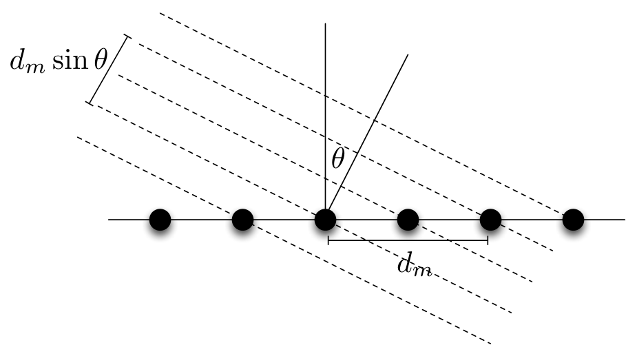
The central theme is that multiple signals are emitted from different locations. Each signal sparsely occupies a bandwidth $W$, and is modulated up to a carrier frequency $\omega_{c}$. A single tone signal $\mathrm{e}^{\iota 2\pi\omega t}$ arrives at multiple array elements record signals with different time shifts, determined by the spacing between array elements as illustrated in Figure 3. As an illustration, the signal arriving at the $m$th array element of an $M$-element array in the simple case of a single emitter is

$\displaystyle x_{m}(t)=\int_{\omega_{c}-W/2}^{\omega_{c}+W/2}\mathrm{e}^{-\iota 2\pi\omega d_{m}\sin\theta/c}\alpha_{m,\omega}\mathrm{e}^{\iota 2\pi\omega t}d\omega,$

(24)

where $\alpha_{m,\omega}\mathrm{e}^{-\iota 2\pi\omega d_{m}\sin\theta/c}:=a_{m}(\theta,\omega)$ is referred to as steering gain at the $m$th array element, where $\mathrm{e}^{-\iota 2\pi\omega d_{m}\sin\theta/c}$ is the phase shift caused in the $\omega$ frequency tone due to the arrival delay $\tau_{m}=d_{m}\sin\theta/c$, and $\alpha_{m,\omega}$ is the gain or strength of $\omega$ tone at $m$th array element. The integral simply aggregate the contributions of frequency components present in the entire bandwidth $W$. The signal ensemble $\bm{X}_{c}(t)$ is the stack of $x_{m}(t),1\leq m\leq M$ as its rows⁶⁶ 6 The elements of the rows are the samples $x_{m}(t_{\ell})$ in a given window of time.. This gives

$\displaystyle\bm{X}_{c}(t)=\int_{\omega_{c}-W/2}^{\omega_{c}+W/2}\bm{a}(\theta,\omega)\mathrm{e}^{\iota 2\pi\omega t}d\omega,$

where the length $M$ column $\bm{a}(\theta,\omega)$ is the steering vector. Evidently, $\bm{a}(\theta,\omega)\mathrm{e}^{\iota 2\pi\omega t}$ is a rank-one ensemble, where we think of the signal $\mathrm{e}^{\iota 2\pi\omega t}$ as a row vector obtained after eventual sampling across time $t$. The ensemble $\bm{X}_{c}(t)$ is obtained by integrating the rank-one ensembles over the narrow-band $W$. The conceptual approach is exactly the same even in the case of multiple emitters as the steering vector $\bm{a}(\bm{\theta},\omega)$ is now a function of multiple incident angles, stacked in a vector $\bm{\theta}$, due to wavefronts from different emitters. However, even in this case the quantity is $\bm{a}(\bm{\theta},\omega)\mathrm{e}^{\iota 2\pi\omega t}$ is still a rank-one ensemble.

The only question that remains to be determined is how the integration over the bandwidth $W$ increases the rank. The answer to this question depends on the density of the array elements compared to the bandwidth $W$. We will show that for narrow-band signals, and high-density arrays, the rank of $\bm{X}_{c}(t)$ remains low. Having an array with a large number of appropriately spaced elements can be very advantageous even when there are only a relatively small number of emitters present. Observing multiple delayed versions of a signal allows us to perform spatial processing, we can beamform to enhance or null out emitters at certain angles, and separate signals coming from different emitters. The resolution to which we can perform this spatial processing depends on the number of elements in the array (and their spacing). For high-density antenna arrays or narrow-band signals, the spatial sampling rate $1/\tau_{m}$ is much larger than the bandwidth $W$. This gives rise to very correlated steering vectors $\bm{a}(\theta,\omega)$. In the standard scenario, where the array elements are uniformly spaced $c/(2\omega_{c})$ along a line, we can make this statement more precise using classical results on spectral concentration [27, 28]. In this case, the steering vectors $\bm{a}(\theta,\omega)$ for $\omega\in[\omega_{c}\pm W/2]$ are equivalent to integer spaced samples of a signal whose (continuous-time) Fourier transform is bandlimited to frequencies in $(1\pm W/(2\omega_{c}))(\sin\theta)/2$, for a bandwidth less than $W/(2\omega_{c})$. Thus the dimension of the subspace spanned by $\{\bm{a}(\theta,\omega),~\omega\in[\omega_{c}\pm W/2]\}$ is, to within a very good approximation, $\approx MW\tau_{m}+1=MW/\omega_{c}+1$.

Figure 3(b) illustrates a particular example. The plot shows the (normalized) eigenvalues of the matrix

$$\bm{R}_{aa}=\int_{\omega_{c}-W/2}^{\omega_{c}+W/2}\bm{a}(\theta,\omega)\bm{a}(\theta,\omega)^{*}\,d\omega,$$

(25)

for the fixed values of $\omega_{c}=5$ GHz, $W=100$ MHz, $c$ equals the speed of light, $M=101$, and $\theta=\pi/4$. We have $MW/\omega_{c}+1=3.02$, and only $3$ of the eigenvalues are within a factor of $10^{4}$ of the largest one.

The correlated signal structure established on the input ensemble is well-known, and many spatial processing tasks, for instance, standard subspace methods [29, 30] for estimating the direction of arrival involve forming the spatial correlation matrix by averaging in time,

$$\bm{R}_{xx}=\frac{1}{L}\sum_{\ell=1}^{L}\bm{X}(t_{\ell})\bm{X}(t_{\ell})^{*}.$$

As the column space of $\bm{R}_{xx}$ should be $\bm{a}(\theta,\omega)$, we can correlate the steering vector for every direction to see which one comes closest to matching the principal eigenvector of $\bm{R}_{xx}$.

The main results of this paper do not give any guarantees about how well these spatial processing tasks can be performed. Rather, they say that the same correlation structure that makes these tasks possible can be used to lower the net sampling rate over time. The entire signal ensemble can be reconstructed from this reduced set of samples, and spatial processing can follow.

On the other hand, the spectral sparsity of the ensemble $\bm{X}_{c}(t)$ is controlled by the active frequencies in the bandwidth $W$, or, more precisely, the joint frequency band occupation of the emitters. It’s easy to imagine several scenarios in practice in automotive radars [31] where the frequency spectrum of the emitters is only sparsely occupied with a priori unknown support. Sparse frequency occupation can also be introduced, for example, when emitters transmit in disjoint frequency bands, and only a subset of the emitters are active at a given time.

It is fair, then, to say that the rank of the signal ensemble is a small constant time the number of narrow band emitters, and each array element can be easily imagined to be recording a very sparsely occupied signal spectrum.

In this section, we numerically simulate the reconstruction of S&L matrix $\bm{H}$ from the given measurements $\bm{Y}_{1}$, and $\bm{Y}_{2}$ in (14) using our proposed algorithm in Section VI. We form a synthetic S&L matrix $\bm{H}$ by multiplying a tall $M\times R$ dense, and a fat $R\times W$ sparse random matrix. The entries of these random matrices are independent Gaussian.

We numerically evaluate the reconstruction algorithm by computing the relative error between the estimate $\hat{\bm{H}}$ in (19), and the ground $\bm{H}$ as follows

$\displaystyle\text{relative error}:=\frac{\|\hat{\bm{H}}-\bm{H}\|_{F}}{\|\bm{H}\|_{F}}.$

(26)

In general, we declare a recovery $\hat{\bm{H}}$ as successful whenever its relative error from the ground truth is less than $10^{-3}$.

To facilitate the discussion, we also introduce the measures of sampling efficiency $\eta$, and compression factor $\gamma$ as follows

$\displaystyle\eta:=\frac{R(M+S-R)}{M_{1}\Omega+M_{2}\Delta}\ \text{and}\ \gamma:=\frac{M_{1}\Omega+M_{2}\Delta}{MW}.$

The sampling efficiency $\eta$ is a ratio of the actual number of degrees of freedom in the unknown S&L matrix $\bm{H}$, and the cumulative number $T=M_{1}\Omega+M_{2}\Delta$ of linear measurements in $\bm{Y}_{1}$ and $\bm{Y}_{2}$; see (14). In other words, sampling efficiency is the ratio between the minimum number of unknown parameters required to completely specify $\bm{X}_{c}(t)$ in $t\in[0,1)$ and the cumulative sampling rate of the proposed scheme. On the other hand, compression factor $\gamma$ is a ratio of the cumulative sampling rate and the Nyquist rate. Since $\eta$, and $\gamma$ are functions of multiple parameters; namely, $R$, $M$, $S$, $M_{1}$, $M_{2}$, $\Omega$, $\Delta$, and $W$. In our experiments, we will often vary $\eta$ by changing only one of these parameters such as $\Delta$, and fixing others, and use the notation $\eta(\Delta)$ to signify that $\eta$ is parametrized by $\Delta$ only while keeping others fixed to known values. Similarly, we will also use $\gamma(\Delta)$ or $\gamma(\Omega)$, etc.

The first set of experiments in Figure 4 shows that successful reconstruction of S&C signal ensemble can be numerically achieved using a rate much smaller than the Nyquist rate. For specific detail, please refer to the image caption.

The second set of experiments in Figure 5 show that the sampling efficiency $\eta(\Delta)$ vs. $S$ settles to $1/8$ after an initial small transition period. Similarly, the sampling efficiency $\eta(\Omega)$ vs. $R$ generally can be expected settles to as high as $1/4$ after an initial transition period. For more specific details on the experimental setup, please refer to the caption of the figure.

The third set of experiments in Figure 6 show phase transitions between compression factor $\gamma(\Omega)$ and sampling efficiency $\eta(R)$; and between compression factor $\gamma(\Delta)$ and sampling efficiency $\eta(S)$. The shade shows the probability of failure; black is the failure probability of 1. We see that in both phase transitions that as the sampling efficiency increases, the compression factor decreases for successful reconstruction. For more specific details on the experimental setup, please refer to the caption of the figure.

The fourth experiment concerns reconstruction in the presence of noise. Figure 7 plots SNR (dB) versus relative error (dB). The relative error of the reconstructed ensemble degrades gracefully with reducing SNR.

In this paper, we propose a novel and implementable sampling architecture for the acquisition of a simultaneously sparse and correlated signal ensemble at a sub-Nyquist rate. The sampling architecture has applications in automotive radars. We prove a sampling theorem showing exact and stable reconstruction of the acquired signals even when the sampling rate is smaller than the Nyquist rate by orders of magnitude. The result of the sampling theorem has been validated via numerical simulations.

Recall that $\bm{L}_{R}$ in (19) are the top-$R$ left singular vectors of $\bm{Y}_{c}$, and let $\bm{V}_{R}$ as in (21) be the top-$R$ right singular vectors of $\bm{H}$. The proof relies on the upper, and lower bounds on the maximum, and minimum singular values, $\sigma_{\max}$ and $\sigma_{\min}$, respectively, of the matrices $\bm{Q}_{1}\bm{V}_{R}$, and $\bm{A}_{2}\bm{L}_{R}$. Lemma 1 in [10] proves that for a fixed $\beta\geq 1$

$\displaystyle\sqrt{\frac{1}{2}}\leq\sigma_{\min}(\bm{Q}_{1}\bm{V}_{R})\leq\sigma_{\max}(\bm{Q}_{1}\bm{V}_{R})\leq\sqrt{\frac{3}{2}}$

(27)

with probability at least $1-\mathcal{O}(W^{-\beta})$ whenever $\Omega\geq c\beta\mu_{0}^{2}R\log^{2}W$. As for $\bm{A}_{2}\bm{L}_{R}$, recall that $\bm{A}$ in (8) was assumed to be a random orthogonal matrix in (6). The orthogonality of $\bm{A}$ has already been used in (V). Since $\bm{A}_{2}$ is a fat random matrix with orthogonal rows, we can write

$$\bm{A}_{2}=(\bm{G}\bm{G}^{*})^{-1/2}\bm{G},$$

where $\bm{G}$ is a standard Gaussian matrix; each entry is iid $\text{Normal}(0,1)$. The matrix $\bm{A}_{2}\bm{L}_{R}=(\bm{G}\bm{G}^{*})^{-1/2}\bm{G}\bm{L}_{R}$, and $\bm{G}\bm{L}_{R}\sim\bm{G}^{\prime}$, where $\bm{G}^{\prime}$ is an $M_{2}\times R$ standard Gaussian matrix. This simply means that

$$\sigma_{\max}(\bm{A}_{2}\bm{L}_{R})\leq\sigma_{\max}(\bm{G}^{\prime})\sigma_{\min}^{-1}(\bm{G}),$$

and

$$\sigma_{\min}(\bm{A}_{2}\bm{L}_{R})\geq\sigma_{\min}(\bm{G}^{\prime})\sigma_{\max}^{-1}(\bm{G}).$$

Using standard result in random matrix theory; see, for example, Corollary 5.35 in [32], the singular values of an $M_{2}\times R$ Gaussian matrix $\bm{G}^{\prime}$ obey

$$\sqrt{M_{2}/2}\approx\sigma_{\min}(\bm{G}^{\prime})\leq\sigma_{\max}(\bm{G}^{\prime})\leq\sqrt{2M_{2}}$$

with probability at least $1-\mathcal{O}(W^{-\beta})$ whenever $M_{2}\geq c(R+\beta\log W)$ for sufficiently large constant $c$. Similarly, we have that

$$\sqrt{M/2}\approx\sigma_{\min}(\bm{G})\leq\sigma_{\max}(\bm{G})\leq\sqrt{2M}$$

with probability at least $1-\mathcal{O}(W^{-\beta})$ whenever $M\geq c(M_{2}+\beta\log W)$. This directly implies that under the same conditions

$\displaystyle 0.5\sqrt{\frac{M_{2}}{M}}\leq\sigma_{\min}(\bm{A}_{2}\bm{L}_{R})\leq\sigma_{\max}(\bm{A}_{2}\bm{L}_{R})\leq 2\sqrt{\frac{M_{2}}{M}}.$

(28)

Equation (27), and (28) directly imply that pseudo inverses $(\bm{Q}_{1}\bm{V}_{R})^{\dagger}$, and $(\bm{A}_{2}\bm{L}_{R})^{\dagger}$ are well defined, where

$\displaystyle(\bm{Q}_{1}\bm{V}_{R})^{\dagger}=\big((\bm{Q}_{1}\bm{V}_{R})^{*}(\bm{Q}_{1}\bm{V}_{R})\big)^{-1}(\bm{Q}_{1}\bm{V}_{R})^{*},$

(29)

and similarly for $(\bm{A}_{2}\bm{L}_{R})^{\dagger}$.

References

- [1] S. M. Patole, M. Torlak, D. Wang, M. Ali, Automotive radars: A review of signal processing techniques, IEEE Signal Processing Magazine 34 (2) (2017) 22–35.
- [2] A. Ahmed, J. Romberg, Compressive sampling of ensembles of correlated signals, arXiv preprint arXiv:1501.06654 (2015).
- [3] A. Ahmed, J. Romberg, Compressive multiplexing of correlated signals, IEEE Trans. Inform. Theory 1 (2015) 479–498.
- [4] R. Sridharan, A. F. Pensa, Us space surveillance network capabilities, in: Image Intensifiers and Applications; and Characteristics and Consequences of Space Debris and Near-Earth Objects, Vol. 3434, International Society for Optics and Photonics, 1998, pp. 88–101.
- [5] P. Maskell, L. Oram, Sapphire: Canada’s answer to space-based surveillance of orbital objects, in: Advanced Maui Optical and Space Surveillance Conference, 2008.
- [6] E. G. Larsson, O. Edfors, F. Tufvesson, T. L. Marzetta, Massive Mimo for next generation wireless systems, IEEE communications magazine 52 (2) (2014) 186–195.
- [7] J. Tropp and J. Laska and M. Duarte and J. Romberg, and R. Baraniuk, Beyond nyquist: Efficient sampling of sparse bandlimited signals, IEEE Trans. Inform. Theory 56 (1) (2010) 520–544.
- [8] J. Laska and S. Kirilos and M. Duarte and T. Raghed and R. Baraniuk and Y. Massoud, Theory and implementation of an analog-to-information converter using random demodulation, in: Proc. IEEE Int. Symp. Circuits Syst., 2007, pp. 1959–1962.
- [9] K. Ding, Z. Meng, Z. Yu, Z. Ju, Z. Zhao, K. Xu, Photonic compressive sampling of sparse broadband rf signals using a multimode fiber, in: 2020 Asia Communications and Photonics Conference (ACP) and International Conference on Information Photonics and Optical Communications (IPOC), 2020, pp. 1–3.
- [10] A. Ahmed, Compressive acquisition and least squares reconstruction of correlated signals, IEEE Signal Processing Letters (2017).
- [11] A. Ahmed, J. Romberg, Compressive sampling of correlated signals, in: 2011 Conference Record of the Forty Fifth Asilomar Conference on Signals, Systems and Computers (ASILOMAR), IEEE, 2011, pp. 1188–1192.
- [12] A. Ahmed, J. Romberg, Compressive multiplexers for correlated signals, in: 2012 Conference Record of the Forty Sixth Asilomar Conference on Signals, Systems and Computers (ASILOMAR), IEEE, 2012, pp. 963–967.
- [13] A. Ahmed, J. Romberg, Compressive sampling in array processing, in: 2013 IEEE 5th International Workshop on Computational Advances in Multi-Sensor Adaptive Processing (CAMSAP), IEEE, 2013, pp. 192–195.
- [14] S. Oymak, A. Jalali, M. Fazel, Y. Eldar, B. Hassibi, Simultaneously structured models with application to sparse and low-rank matrices, IEEE Trans. Inform. Theory 61 (5) (2015) 2886–2908.
- [15] C. R. Schlottmann, P. E. Hasler, A highly dense, low power, programmable analog vector-matrix multiplier: The fpaa implementation, IEEE Journal on emerging and selected topics in circuits and systems 1 (3) (2011) 403–411.
- [16] R. Chawla, A. Bandyopadhyay, V. Srinivasan, P. Hasler, A 531 nw/mhz, 128/spl times/32 current-mode programmable analog vector-matrix multiplier with over two decades of linearity, in: Custom Integrated Circuits Conference, 2004. Proceedings of the IEEE 2004, IEEE, 2004, pp. 651–654.
- [17] M. Mishali and Y. Eldar, Blind multiband signal reconstruction: Compressed sensing for analog signals, IEEE Trans. Sig. Process. 57 (3) (2009) 993–1009.
- [18] N. Halko, P.-G. Martinsson, J. A. Tropp, Finding structure with randomness: Probabilistic algorithms for constructing approximate matrix decompositions, SIAM review 53 (2) (2011) 217–288.
- [19] J. Slavinsky, J. Laska, M. Davenport, R. Baraniuk, The compressive multiplexer for multi-channel compressive sensing, in: Proc. IEEE Int. Conf. Acoust., Speech, and Sig. Process. (ICASSP), Prague, Czech Republic, 2011, pp. 3980–3983.
- [20] E. J. Candès, M. B. Wakin, An introduction to compressive sampling, IEEE signal processing magazine 25 (2) (2008) 21–30.
- [21] J.-L. Starck, F. Murtagh, J. M. Fadili, Sparse image and signal processing: wavelets, curvelets, morphological diversity, Cambridge university press, 2010.
- [22] M. Mishali and Y. Eldar and O. Dounaevsky and E. Shoshan, Xampling: Analog to digital at sub-Nyquist rates, IET Circuits Devices Syst. 5 (1) (2011) 8–20.
- [23] F. Wang, J. Fang, H. Duan, H. Li, Phased-array-based sub-nyquist sampling for joint wideband spectrum sensing and direction-of-arrival estimation, IEEE Transactions on Signal Processing 66 (23) (2018) 6110–6123.
- [24] B.-H. Ku, P. Schmalenberg, S. Y. Kim, C.-Y. Kim, O. Inac, J. S. Lee, K. Shiozaki, G. M. Rebeiz, A 16-element 77–81-ghz phased array for automotive radars with50° beam-scanning capabilities, in: 2013 IEEE MTT-S International Microwave Symposium Digest (MTT), IEEE, 2013, pp. 1–4.
- [25] R. A. Alhalabi, G. M. Rebeiz, A 77-81-ghz 16-element phased-array receiver with50° beam scanning for advanced automotive radars [j], IEEE Transaction on Microwave Theory and Techniques 62 (11) (2014) 2823–2832.
- [26] J. G. Miller, A new sensor allocation algorithm for the space surveillance network, Military Operations Research (2007) 57–70.
- [27] D. Slepian, On bandwidth, Proceedings of the IEEE 64 (3) (1976) 292–300.
- [28] D. Slepian, Prolate spheroidal wave functions, fourier analysis and uncertainty v — the discete case, Bell Systems Tech. Journal 57 (1978) 1371–1430.
- [29] R. O. Schmidt, Multiple emitter location and signal parameter estimation, IEEE Trans. Antennas Propag. AP-34 (1986) 276–280.
- [30] R. Roy, T. Kailath, Esprit-estimation of signal parameters via rotational invariance techniques, IEEE Trans. Acoust., Speech, Sig. Process. 37 (7) (1989) 984–995.
- [31] G. Feinberg, S. Mulleti, E. Shoshan, Y. C. Eldar, Hardware prototype demonstration of a cognitive sub-nyquist automotive radar, Electronics Letters 55 (9) (2019) 556–558.
- [32] R. Vershynin, Compressed sensing: theory and applications, Cambridge University Press, 2012.
- [33] M. Rudelson, R. Vershynin, On sparse reconstruction from fourier and gaussian measurements, Commun. Pure Appl. Math. 61 (8) (2008) 1025–1045.