A Survey for High-Mass Eclipsing Binaries2019A Survey for High-Mass Eclipsing Binaries–9

F. Pozo Nuñez Thanks: E-mail: francisco.pozon@gmail.com Affiliation: Astronomisches Institut, Ruhr–Universität Bochum, Universitätsstraße 150, 44801 Bochum, Germany. Affiliation: Centrum Astronomiczne im. Mikolaja Kopernika, PAN, Bartycka 18, 00-716 Warsaw, Poland. R. Chini Affiliation: Astronomisches Institut, Ruhr–Universität Bochum, Universitätsstraße 150, 44801 Bochum, Germany. Affiliation: Instituto de Astronomía, Universidad Católica del Norte, Avenida Angamos 0610, Casilla 1280,Antofagasta, Chile. A. Barr Domínguez Affiliation: Centro de Investigación Multidisciplinario de la Araucanía, Facultad de Ingeniería, Universidad Autonoma de Chile, AvenidaAlemania 01090, Temuco, Chile. Ch. Fein Affiliation: Astronomisches Institut, Ruhr–Universität Bochum, Universitätsstraße 150, 44801 Bochum, Germany. M. Hackstein Affiliation: Astronomisches Institut, Ruhr–Universität Bochum, Universitätsstraße 150, 44801 Bochum, Germany. Pietrzyński Grzegorz Affiliation: Centrum Astronomiczne im. Mikolaja Kopernika, PAN, Bartycka 18, 00-716 Warsaw, Poland. M. Murphy Affiliation: Departamento de Física, Universidad Católica del Norte, Avenida Angamos 0610, Casilla 1280 Antofagasta, Chile

Accepted 2019 October 16. Received 2019 October 13; in original form 2019 March 01

Abstract

We report results from a search for Galactic high-mass eclipsing binaries. The photometric monitoring campaign was performed in Sloan $r$ and $i$ with the robotic twin refractor RoBoTT at the Universitätssternwarte Bochum in Chile and complemented by Johnson $UBV$ data. Comparison with the SIMBAD database reveals 260 variable high-mass stars. Based on well-sampled light curves we discovered 35 new eclipsing high-mass systems and confirm the properties of six previously known systems. For all objects, we provide the first light curves and determine orbital periods through the Lafler-Kinman algorithm. Apart from GSC 08173-0018 and Pismis 24-13 ( $P=19.47\,d$ and $20.14\,d$ ) and the exceptional short-period system TYC 6561-1765-1 ( $P=0.71\,d$ ), all systems have orbital periods between 1 and 9 days. We model the light curves of 26 systems within the framework of the Roche geometry and calculate fundamental parameters for each system component. The Roche lobe analysis indicates that 14 systems have a detached geometry while 12 systems have a semi-detached geometry; seven of them are near-contact systems. The deduced mass ratios $q=M_{2}/M_{1}$ reach from 0.4 to 1.0 with an average value of 0.8. The similarity of masses suggests that these high-mass binaries were created during the star formation process rather than by tidal capture.

Keywords:

stars: fundamental parameters – stars: formation – binaries: eclipsing – binaries: spectroscopic – Galaxy: open clusters and associations

1 Introduction

There is growing evidence that a large fraction of the total stellar population consists of binary and multiple stars (Duchêne & Kraus 2013). The role of such systems for astrophysics is tremendous because they provide the most accurate data about the basic stellar properties like mass, radius, luminosity, projected rotational velocity or abundances. At the same time, binary and multiple systems are crucial for studying gas dynamics, accretion processes, and interaction of stellar winds. Most notably, the formation of binaries and multiple systems remain major unsolved problems (e.g. Zinnecker 2003; Tokovinin 2008; Boss 2014). Interestingly, high-mass stars seem to have the highest multiplicity rate among all stars which increases the chance to be observed as eclipsing binary (EB) systems. As a consequence early-type EBs are not only a unique laboratory to study the formation and evolution of stars but – due to their brightness – they have even the potential for measuring accurate distances to nearby galaxies (e.g. Bonanos 2013).

During recent years many stars which were treated as singles for many decades turned out to be double or multiple systems when taking a closer look. This is true for the immediate solar neighbourhood ( $d<25$ pc) where well known F-type stars are found to form binary or hierarchical systems (Halbwachs et al. 2003; Fuhrmann & Chini 2012; Chini et al. 2013; Fuhrmann et al. 2017, e.g.), rising the multiplicity fraction for solar type stars to about 58%. For A-type stars, De Rosa et al. 2014 derive a companion star fraction of $68.9\pm 7$ %.

Recent surveys for O-type stars have revealed multiplicity fractions of 50% to more than 80%. (Chini et al. 2012; Sana et al. 2012; 2013A&A...550A.107S; Sota et al. 2014; Maíz Apellániz et al. 2016, e.g.) and led to the assumption that only a small fraction of stars above $20\,M_{\odot}$ are born as single stars. Multiplicity surveys for B-type stars are less frequent (Schöller et al. 2012; Chini et al. 2012; Dunstall et al. 2015, e.g.) but it seems that their properties such as period and mass-ratio follow those of O-type stars. Obviously, although the fraction of high-mass stars in a galaxy is a minor portion of the total stellar content their multiplicity fraction appears to be the highest among all stellar masses. This peculiarity is not yet understood and requires further investigation.

Eventually, orbital period and mass-ratio provide significant constraints on models of star formation and evolution. Thus, apart from knowing the masses of the components in a multiple system, orbital parameters are important to understand the formation of high-mass stars. The multiplicity surveys for high-mass stars have revealed mass ratios $q=M_{2}/M_{1}$ close to unity and typical periods of only a few days suggesting that the evolution of members of multiple systems must differ significantly from that of a single high-mass star. This holds for the formation scenarios (fragmentation, disk-instabilities), the evolution (mass-transfer, merging) and the corresponding final states (blue stragglers, X-ray binaries, gamma-ray bursts). 2013A&A...550A.107S estimated that more than 50% of the current O-star population will exchange mass with its companion within a binary system. Assuming a constant star formation rate, de Mink et al. 2014 found that 8% of a sample of early-type stars are the product of a merger event in a close binary system. In total they estimate that 30% of massive main-sequence stars are the product of binary interaction.

Concerning the formation of multiple high-mass stars the sequence of events, from the fragmentation of cloud cores to the dynamical interaction and orbit migration of stellar components, seems well established. Still, theoretical predictions for the formation of multiple systems and the evolution of their orbits into their present configuration of a tight inner binary and possibly a much more distant third component vary widely, depending on the initial conditions, physical processes involved or modelled and computational details. The most important aspects are briefly reviewed in the following:

•

Cascade fragmentation. Fragmentation is believed to be the dominant mechanism forming binary and multiple stars. Krumholz et al. 2007 present radiation-hydrodynamic simulations of collapse and fragmentation to investigate whether massive protostellar cores form a small or large number of protostars. Interestingly, it is found that radiation feedback from the first few accreting protostars inhibits the formation of further fragments within the cloud core. In other words, the majority of the collapsing mass accretes onto one or a few objects. In a second step, further fragmentation may occur in massive, self-shielding disks which are driven to gravitational instability by rapid accretion. Whether the accreting gas is transported to the central star or increases the mass of the fragment inside the disk depends on the model calculations. In any case these results demonstrate that massive cores with observed properties are not likely to fragment into many stars.
•

Accretion. Binary protostars produced by fragmentation during the isothermal cloud collapse have separations between $10^{2}$ and $10^{4}$ AU (e.g. Sterzik et al. 2003). The final properties of a multiple system will be determined by the ongoing accretion of gas. Numerous hydrodynamical simulations show that accretion leads to similar-mass components (Halbwachs et al. 2003; Söderhjelm 2007).
•

N-body dynamics. Calculations (e.g. Goodwin & Kroupa 2005 and references therein) show that it is not possible to reproduce the observed multiplicity fraction through the dynamical evolution of star clusters that are born with a single-star population. While dynamical interactions may disrupt many wide binaries they are neither able to pair stars efficiently nor to change the properties of close binaries significantly. Taking into account also the observed separations of multiple systems the authors argue that of every 100 star-forming cores in a molecular cloud about 60 will produce binaries while 40 will produce triple systems. Among the latter group 25 are long-lived hierarchical systems while 15 will decay into 15 binaries and 15 single stars - predominantly of low mass which will be ejected. Thus both observations and theory lead to the conclusion that star-forming cores must typically produce only 2 or 3 physically bound stars. This result is in contrast to many numerical simulations that predict the formation of $5-10$ stars per core.

Delgado-Donate et al. 2004 performed particle hydrodynamics and $N-$ body simulations of fragmenting cores. They find that 80% of the forming stars are members of multiples systems, with component separations between 1 and 1000 AU; this fraction is an increasing function of primary mass. The multiple systems consist of binaries and triples, where the mass ratio within binaries attain typical values of $0.5-1$ . With increasing time dynamics disrupt mostly wide and/or low-mass companions with low binding energies, but has little effect on the inner subsystems with high-mass components.
•

Dynamical interactions and orbital decay. The formation of close binary systems by dynamical interactions and orbital decay was studied by Bate et al. 2002. Their hydrodynamical star formation calculation shows that close binaries with separations $\leq 10$ AU need not be formed directly by fragmentation but could be the result of a combination of dynamical interactions in unstable multiple systems and the orbital decay of initially wider binaries. Orbital decay may be due to gas accretion and/or the interaction of a binary with its circum-binary disk. The interesting aspect of this scenario is the fact that close binaries with roughly equal-mass components are formed. This is because dynamical exchange interactions and the accretion of gas with high specific angular momentum drive mass ratios towards unity. Another consequence of dynamical interactions is the tendency that stars of higher mass should have a higher frequency of close companions.

Tokovinin 2008 compared the statistics of triple and quadruple stars. According to the observations the properties of multiple stars are not compatible with the dynamical decay of small clusters which would imply that $N-$ body dynamics is not the dominant process of their formation. In contrast, (cascade) fragmentation possibly followed by migration of inner and/or outer orbits could explain the observations of triple and quadruple stars.
•

Kozai cycles with tidal friction. Many binary stars have separations of only a few stellar radii. This implies that their orbits must have shrunk by $1-2$ orders of magnitude after their formation because the radius of a star also shrank considerably from its birth to the main sequence. Orbital shrinkage was investigated by Fabrycky & Tremaine 2007 who considered the effects of secular perturbations from a distant companion star (so-called Kozai cycles) and tidal friction. Kozai 1962 discovered that the amplitude of both the eccentricity and the inclination of the inner system oscillates – independent of the strength of the perturbation from the outer body. The oscillation amplitude only depends on the initial mutual inclination between inner and outer binaries; for the extreme case of an initial inclination of $90^{\circ}$ the maximum eccentricity becomes 1, i.e. the two inner bodies will collide. Separations less than a few stellar radii – as they may occur during some phase of a Kozai cycle – imply a tidal friction that drains energy from the orbit, reducing the semi-major axis even more. Fabrycky & Tremaine 2007 find that binaries with orbital periods of $0.1-10$ days are produced from binaries with much longer initial periods (10 to $\sim 10^{5}$ days). This result is consistent with the observation that short-period binaries are often accompanied by a third star.

The huge progress provided by spectroscopic and interferometric surveys can be complemented by photometric searches for high-mass EBs because they can provide system properties that are not accessible through spectroscopy alone due to the unknown inclination of the systems. Therefore, finding high-mass EBs is a major step ahead in our understanding of the properties of these exotic systems. Interestingly, to our knowledge, the literature describes only 18 high-mass EBs (Rauw et al. 2001, Freyhammer et al. 2001, Sana et al. 2003, Sana et al. 2006, Hillwig et al. 2006, Niemela et al. 2006, Barr Domínguez et al. 2013 (hereafter called Paper I), Kobulnicky et al. 2014, Kiminki et al. 2015, Mayer et al. 2017). The three high-mass EBs systems from Paper I – HD 319702 (O+B), CPD-51 8946 (O+B), and Pismis 24-1 (O+O) – were discovered in the framework of our long-term photometric Bochum Galactic Disk Survey (GDS; Hackstein et al. 2015, Kaderhandt et al. 2015).

The present paper reports the complete high-mass star results from the GDS which comprise 473 stars crudely classified as OB in the literature. Among those are 263 variable sources that we analyze for the presence of EBs on the basis of their light curves. For the detected EBs we complement the GDS standard photometry in Sloan $r$ and $i$ by new $UBV$ data and present photometric spectral types, light curves and periods for all systems.

Table 1: Characteristics of the observed high-mass eclipsing binaries.

No.	Name	RA	Dec	spectral designations	references
		J2000
1	CPD $-$ 24° 2836	07 45 33.18	-24 42 03.29	O9-B0	$a$
2	CPD $-$ 26° 2656	07 50 18.04	-27 15 03.40	B1:V:, OB:, B0V, B5V	$a,b,c,d$
3	TYC 6561-1765-1	07 52 20.09	-27 04 56.23	O9.5	$c$
4	CD $-$ 31° 5524	08 05 55.87	-31 48 30.62	OB, O9/9.5	$o,p$
5	CPD $-$ 42° 2880	08 44 26.45	-43 10 02.48	O9.5-B2	$a$
6	CPD $-$ 45° 3253	08 55 38.09	-46 21 38.47	B0:, OB⁰?, O9:	$a,e,f$
7	GSC 08156-03066	08 56 25.90	-48 24 35.47	OB⁰	$e$
8	GSC 08173-00182	09 09 53.72	-48 51 56.20	OB⁺	$e$
9	TYC 8175-685-1	09 22 39.17	-49 02 10.04	OB⁺	$e$
10	ALS 18551	10 58 17.00	-61 11 54.00	O4.5	$h$
11	CPD $-$ 39° 7292	17 13 24.46	-39 47 42.68	OB⁺, B1V, B1IIIn?	$i,j,k$
12	Pismis 24-4	17 24 40.49	-34 12 06.51	O9-B0?	$g$
13	CD $-$ 29° 14032	17 49 09.40	-29 14 33.20	B1III	$k$
14	SS 117	07 27 31.64	-13 38 41.30	OB^-	$l$
15	CD $-$ 33° 4174	07 48 38.55	-33 51 00.60	OB, OB⁺	$m,l$
16	CD $-$ 28° 5257	08 00 03.26	-28 50 25.91	O8, O9.5V	$d,n$
17	LS 1221	08 59 50.56	-47 24 31.39	OB^-, OB⁰	$o,e$
18	CD $-$ 51° 10200	16 28 09.45	-51 31 08.07	OB	$o$
19	GSC 07380-00198	17 36 15.59	-33 31 28.70	OB^-	$q$
20	ALS 17569	08 59 19.42	-48 19 51.50	OB?	$e$
21	HD 300214	09 45 25.92	-54 22 09.47	O, B7	$o,r$
22	TYC 8958-4232-1	10 58 45.47	-61 10 43.00	O5Ifp	$s$
23	HD 308974	11 41 31.39	-61 50 03.59	OB	$t$
24	CPD $-$ 54° 7198	16 12 27.00	-54 29 43.80	OB	$u$
25	HD 152200	16 53 51.63	-41 50 32.55	O9.7IV(n)	$s$
26	TYC 6265-2079-1	18 22 03.13	-15 46 21.98	OB, B3/B4	$v,w$
27	BD $-$ 024786	18 56 03.64	-02 37 35.36	OBe	$x$
28	ALS 15204	10 43 41.24	-59 35 48.18	O7.5V	$h$
29	V 467 Vel ^∗	08 43 49.81	-46 07 08.78	O6.5V	$h$
30	HD 92607 ^∗	10 40 12.43	-59 48 10.10	O9IV	$h$
31	CPD $-$ 59° 2603 ^∗	10 44 47.31	-59 43 53.23	O7.5V, B0V(n)	$y$
32	CPD $-$ 59° 2628 ^∗	10 45 08.23	-59 40 49.48	O9.5V, B0.5V(n)	$h$
33	CPD $-$ 59° 2635 ^∗	10 45 12.72	-59 44 46.17	O8V, O9.5V	$h$
34	V662 Car ^∗	10 45 36.32	-59 48 23.37	O5V, B0:V	$h$
35	EM Car ^∗	11 12 04.50	-61 05 42.94	O7.5V, O7.5V	$h,z$
36	HD 115071 ^∗	13 16 04.80	-62 35 01.47	O9.5III, B0Ib	$h$
37	HD 152219 ^∗	16 53 55.61	-41 52 51.47	O9.5III	$h$
38	CD $-$ 41° 11042 ^∗	16 54 19.85	-41 50 09.36	O9.2IV, B1:V	$h$
39	TYC 7370-460-1 ^∗	17 18 15.40	-34 00 05.94	O6V, O8V	$h$
40	HDE 323110 ^∗	17 21 15.79	-37 59 09.58	ON9Ia	$h,z$
41	Pismis 24-13 ^∗	17 24 45.79	-34 09 39.94	O6V	$h$

Notes: $a$ : Nordström 1975, $b$ : Lodén 1966, $c$ : Peton-Jonas 1981, $d$ : Reed & Fitzgerald 1983, $e$ : Muzzio & Orsatti 1977, $f$ : Slawson & Reed 1988, $g$ : Wang et al. 2007, $h$ : Maíz Apellániz et al. 2016, $i$ : Drilling 1991, $j$ : Dachs et al. 1982, $k$ : Vijapurkar & Drilling 1993, $l$ : Stephenson & Sanduleak 1977, $m$ : Orsatti 1992, $n$ : Crowther et al. 2006, $o$ : Stephenson & Sanduleak 1971, $p$ : Sundman et al. 1974, $q$ : Moffat et al. 1977, $r$ : Reed 2003, $s$ : Sota et al. 2014, $t$ : Lyngå 1969, $u$ : Drilling 1968, $v$ : Stephenson & Hobbs 1961, $w$ : Povich et al. 2009, $x$ : Nassau & Stephenson 1963, $y$ : Rauw et al. 2001, $z$ : Pojmanski 2003. ^∗ stars from the Galactic O-Star Catalogue (Maíz Apellániz et al. 2016) identified as EBs in the present work.

2 Observations

2.1 Sample selection

Refer to caption — Figure 1: Distribution of magnitudes (left) and amplitudes (right) for 263 variable high-mass stars in $r$ (blue) and $i$ (red).

The GDS comprises $\sim 16$ million stars of which $\sim 85.000$ are variable. The variability selection procedure was based on three methods: i) Stetson variability $J$ -index ( $J$ -method, Stetson 1996; ii) amplitude method ( $\delta_{\rm A}$ ) which corresponds to the difference between minimum and maximum brightness in the time series, and iii) standard deviation ( $\sigma_{\rm LC}$ ; SD-method) of the light curves. A full description of the identification of variable objects can be found in Hackstein et al. 2015. In brief, since the $\delta_{A}$ and SD methods are sensitive to the scatter in the light curves, they have to be determined as a function of brightness ( $m$ ). We therefore used a 5 $\sigma$ threshold applied to an $8^{th}$ degree polynomial fit $\sigma_{fit}(m)$ where $a_{fit}(m)$ was obtained from both $\delta_{A}-m$ and $\sigma_{\rm LC}-m$ diagrams, respectively. A source is considered as variable if the condition $\sigma_{\rm LC}>\sigma_{\rm fit}(m)+5\ \sigma_{\rm SD}$ is satisfied for the SD method or if $\delta_{A}>a_{fit}(m)+5\ \sigma_{\delta_{A}}$ is satisfied for the $\delta_{\rm A}$ method. In the case of the Stetson $J$ -index, a threshold value of $0.5$ was used (Fruth et al. 2012). Therefore, a source is considered as variable if the condition $|J|>0.5$ is satisfied. Due to systematic errors, the $J$ -index usually finds positive detections for objects with very low amplitudes, hence, an additional condition based on the $\delta_{\rm A}$ method was also introduced. Finally, a source is considered as variable if a variability flag is raised by at least one of the previous methods.

By matching all detected sources with the SIMBAD catalogue we found 473 O-type stars of which 263 are variable. The matching was performed using an optimal 3" search radius, which is a good compromise between the varying positional accuracies in the SIMBAD database and a minimisation of multiple matches. Figure 1 shows the distribution of magnitudes and variability amplitudes for 263 O-type stars.

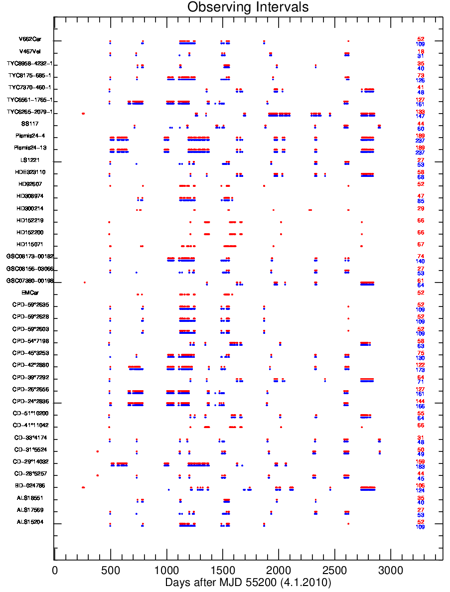
We performed a second match between the variable O-type stars that were previously identified in SIMBAD database (263) and the Galactic O-Star Catalogue (GOSC¹¹ 1 Here we use the latest 4.1 version of the catalogue (June 2018), which list 594 O-type stars. See https://gosc.cab.inta-csic.es/., Maíz Apellániz et al. 2016). We find a match with 83 sources, including two EBs from Paper I (Pismis 24-1 and HD 319702), with magnitudes ranging between $\sim 7-12$ mag and $\sim 9-14$ mag in the $r$ and $i$ filters, respectively. Figure 2 shows the distribution of magnitudes and variability amplitude for 83 identified GOSC stars. From the identified GOSC stars, we find that 25 sources show periodic variations among them 13 systems with well defined eclipses. Among all identified high-mass stars we found 41 EB systems (14%). After the light curves have been folded with the corresponding period, a system is considered as EB when it shows well-defined primary and secondary minima. Six EBs were known before and we confirm the previous results; the remaining 35 systems are new discoveries. The three sources from Paper I were omitted from this statistics. Table 1 lists the EBs and their positions. We present the observational time span of the EB systems in the Appendix (Figure 9).

2.2 Data

The GDS observations were performed with the 15 cm Robotic Bochum Twin Telescope (RoBoTT) of the Universitätssternwarte Bochum, located near Cerro Armazones in Chile. The high-mass stars from the present work comprehend observations obtained from 268 fields along the galactic plane between 2009 and 2018 (Hackstein et al. 2015). The photometric monitoring was conducted simultaneously in the Sloan $r$ (6230 Å) and $i$ (7616 Å) filters. For several stars, we performed additional single-epoch Johnson $UBV$ observations.

The data reduction was standardized, including bias, dark current, flatfield, astrometry and astrometric distortion corrections performed with IRAF²² 2 IRAF is distributed by the National Optical Astronomy Observatory, which is operated by the Association of Universities for Research in Astronomy (AURA) under cooperative agreement with the National Science Foundation. in combination with SCAMP (Bertin 2006) and SWARP (Bertin et al. 2002) routines.

The photometry was done with the DAOPHOT routine from IRAF, using an aperture radius of 4"; this choice maximized the signal-to-noise ratio and delivered the lowest absolute scatter for the fluxes. The brightness of the variable program stars was calculated relative to nearby non-variable reference stars located in the same field. The absolute photometric calibration was obtained from fluxes of about 20 standard stars (Landolt 2009) observed during the same nights as the science targets (see Paper I for more information).

The number of epochs during the monitoring campaign as well as the photometric $UBV$ results are summarized in the Appendix in Table 8.

3 Data analysis

3.1 Spectral types

Tab. 1 lists the existing spectral designations which are sometimes coarse or doubtful as described in the original literature; nevertheless, the sample includes only high-mass stars. Therefore, we also used the single-epoch $UBV$ data to obtain a photometric classification in parallel. For the identified sub-sample of GOSC stars, we used the spectral types as listed in the latest release of the catalogue. Fig. 3 corroborates that all objects are OB-type stars by their $UBV$ colors. When dereddening the stars via the reddening path $E_{U-B}/E_{B-V}$ = $0.72$ + $0.05E_{B-V}$ (Hiltner & Johnson 1956), we obtain spectral types from O9 to B7. The photometric solution for star No. 1 is not unique; given, however, the spectroscopic classification of O9-B0 (Nordström 1975) we prefer the earliest solution.

Generally one must note that in the case of a binary the observed colors are a combination of the flux contributions from two stars. Depending on the mass ratio $q=M_{2}/M_{1}$ of the components the combined colors will either agree with the colors of the primary ( $q=1$ ) or they will be redder ( $q<1$ ). In the latter case, the combined photometric spectral type will be later than the spectroscopic type of the primary. This problem will be discussed more thoroughly with the individual sources.

3.2 Light curve Modelling

The light curves were analysed assuming a standard Roche geometry based on the Wilson-Devinney (WD) code (Wilson & Devinney 1971, Wilson 1979, Wilson 1990). The modelling procedure is explained in detail in Paper I; here we describe only its main characteristics. First, the orbital periods were determined using the Lafler-Kinman algorithm (Lafler & Kinman 1965) which was later generalized and introduced as Phase Dispersion Minimization (PDM) by Stellingwerf 1978. The PDM is performed on a period range from 0.1 to $\sim 70$ days. The choice of the lower limit is a compromise between the minimum value of $\sim 0.14$ days obtained by Drake et al. 2014 for ultra-short period binaries from the Catalina Survey, and the short-period limit of $\sim 0.22$ days for contact binary systems reported by Rucinski 1992. The upper limit has a range of $13<P<119$ days and is dynamically calculated so that the analyzed maximum period should be $T/2$ , with $T$ the length of the time series for the particular light curve. We must note that any algorithm used to find the periods of EBs is sensitive to the total number of observations and time sampling of the light curves. An efficiency test performed on the PDM method is presented in Appendix A. Then, the effective temperature of the primary component was calculated for an adopted spectral type taking into account the spectral information (Tab. 1) and our $UBV$ data (Tab. 8) assuming all stars to be on the main sequence. For the conversion between spectral type and effective temperature we used the values from Theodossiou & Danezis 1991.

The symmetrical separation of the primary and secondary minimum eclipses for all stars in the present sample suggests that these systems have fairly circular orbits. We therefore assumed zero eccentricity and synchronous rotation for all model fits. In the case of circular orbits and synchronous rotation, the Roche equipotential ( $\Omega$ ) along with the mass ratio ( $q$ ) describe the surface structure or Roche lobe of both components in the EB system. The geometric classification of an EB, whether the system is detached, semi-detached, contact or overcontact, depends on $\Omega$ and the commonly used fill-out factor $f$ . The factor $f$ is expressed in terms of the inner ( $\Omega_{in}$ ) and outer ( $\Omega_{out}$ ) critical Roche equipotentials. For a detached system, the factor $f$ is defined by $f=(\Omega_{in}/\Omega)-1$ for $\Omega_{in}<\Omega$ , and will lie between $-1<f\leq 0$ . For a contact binary, $f$ takes the value $f=(\Omega_{in}-\Omega/\Omega_{in}-\Omega_{out})$ for $\Omega_{in}\geq\Omega$ , and will lie between $0\leq f\leq 1$ (Wilson 1979, Wilson 1990, but see also Leahy & Leahy 2015). For simplicity, and to be able to work with positive values, we defined the Roche Lobe Coefficient (RLC) $F=f+1$ which corresponds to the values listed in Table 3.

Table 2: EB systems without modelling.

No.	Name	$P$ [d]
14	SS 117	$2.00930\pm 0.00210$
15	CD $-$ 33° 4174	$4.47699\pm 0.00103$
16	CD $-$ 28° 5257	$1.50698\pm 0.00323$
17	LS 1221	$1.14928\pm 0.00042$
18	CD $-$ 51° 10200	$1.12509\pm 0.00063$
19	GSC 07380-00198	$7.64607\pm 0.00291$
20	ALS 17569	$5.26895\pm 0.00184$
21	HD 300214	$2.02429\pm 0.00022$
22	TYC 8958-4232-1	$5.10888\pm 0.00051$
23	HD 308974	$4.74915\pm 0.00021$
24	CPD $-$ 54° 7198	$4.29379\pm 0.00034$
25	HD 152200	$8.89365\pm 0.00081$
26	TYC 6265-2079-1	$3.67867\pm 0.00073$
27	BD $-$ 024786	$2.52880\pm 0.00124$
28	ALS 15204	$2.23266\pm 0.00030$

Notes: The numbers given in the first column correspond to the numbers used in Table 1.

Gravity-darkening coefficients $\beta_{1}=\beta_{2}=0.25$ and bolometric albedos $A_{1}=A_{2}=1.0$ were taken for early-type stars with radiative envelopes and hydrostatic equilibrium. We used a nonlinear square-root limb darkening law obtained at optical wavelengths (Diaz-Cordoves & Gimenez 1992) with limb darkening coefficients interpolated from tables of van Hamme 1993 at the given band pass. The best model was determined through repeated fits to the light curves until the minimum of $\chi^{2}$ was reached. During the fitting procedure the following adjustable parameters were optimized in each iteration: the effective temperature of the secondary star, the Roche lobe filling factors for the primary and secondary star, the inclination of the system and the photometric mass ratio ( $q$ ) using the $q-$ search method.

Since there are no spectroscopic mass ratios available for the systems in this study, we first searched for a reasonable starting value for $q$ . Adopting mass-ratios from 0.10 to 1.0 in steps of 0.05 we obtained light curve solutions; the resulting sum of the squared deviations ( $\chi^{2}$ ) for each value of $q$ was analysed. The value of $q$ corresponding to the minimum of $\chi^{2}$ obtained for each binary star was taken as the most plausible starting point for the mass-ratio. Figure. 4 shows as an example the relation between $\chi^{2}$ and $q$ for the star CPD -26° 2656. The lowest value of the residuals occurred at around $q=0.85$ . Once the starting point for the mass ratio was determined by the $q-$ search method, $q$ was taken as a free parameter along with the other parameters to obtain the final solution.

Table 3: Orbital solutions and system parameters.

Results	CPD -24° 2836	CPD -26° 2656	TYC 6561-1765-1	CPD -42° 2880	CPD -45° 3253	GSC 08156-03066	GSC 08173-00182
$P$ [d]	$1.02\pm 0.007$	$2.699\pm 0.007$	$0.712\pm 0.001$	$1.90\pm 0.009$	$6.68\pm 0.009$	$2.3318\pm 0.006$	$19.47\pm 0.009$
$T_{0}$	$55971.168507$	$55968.14481$	$55927.26512$	$55984.204734$	$56236.345903$	$56314.182400$	$56333.182049$
$M_{2}/M_{1}$	$0.416\pm 0.076$	$0.856\pm 0.102$	$0.753\pm 0.079$	$0.612\pm 0.083$	$0.624\pm 0.087$	$0.996\pm 0.096$	$0.714\pm 0.088$
$i$	$57\aas@@fstack{\circ}3\pm 2\aas@@fstack{\circ}1$	$79\aas@@fstack{\circ}7\pm 1\aas@@fstack{\circ}6$	$55\aas@@fstack{\circ}7\pm 1\aas@@fstack{\circ}7$	$64\aas@@fstack{\circ}8\pm 1\aas@@fstack{\circ}8$	$64\aas@@fstack{\circ}1\pm 2\aas@@fstack{\circ}1$	$52\aas@@fstack{\circ}4\pm 1\aas@@fstack{\circ}4$	$59\aas@@fstack{\circ}5\pm 1\aas@@fstack{\circ}7$
RLC(1)	$0.860\pm 0.011$	$0.650\pm 0.007$	$0.880\pm 0.009$	$0.730\pm 0.008$	$0.730\pm 0.012$	$0.932\pm 0.011$	$0.890\pm 0.013$
RLC(2)	$0.840\pm 0.010$	$0.740\pm 0.005$	$0.642\pm 0.005$	$0.720\pm 0.007$	$0.720\pm 0.012$	$0.928\pm 0.009$	$0.870\pm 0.012$
$T_{1}$ [K]	$29\,230$	$25\,570$	$18\,445$	$29\,230$	$29\,230$	$25\,570$	$18\,445$
$T_{2}$ [K]	$19\,520\pm 1510$	$23\,250\pm 1112$	$13\,150\pm 1180$	$22\,110\pm 1120$	$22\,250\pm 1302$	$24\,150\pm 1290$	$13\,920\pm 1260$
$\Delta D_{p}$	$7.5\%$	$33.5\%$	$6.0\%$	$8.5\%$	$9.0\%$	$10.0\%$	$12.5\%$
$\Delta D_{s}$	$5.5\%$	$28.5\%$	$5.0\%$	$5.5\%$	$6.0\%$	$9.0\%$	$10.5\%$

Notes: $P$ is the orbital period (in days) obtained from the PDM analysis; The reference time $T_{0}$ refers to the time of the primary eclipse (HJD-2400000); $M_{2}/M_{1}$ is the mass ratio; $i$ the orbital inclination. RLC(1) and RLC(2) are the Roche Lobe Coefficients, $T_{1}$ and $T_{2}$ are the effective temperatures, and $\Delta D_{p}$ and $\Delta D_{s}$ correspond to the amplitude of the minima for the primary and secondary component, respectively.

Table 4: continued

Results	TYC 8175-685-1	ALS 18551	CPD $-$ 39° 7292	Pismis 24-4	CD $-$ 29° 14032	CD $-$ 31° 5524	V 467 Vel
$P$ [d]	$3.4085\pm 0.009$	$1.360\pm 0.006$	$2.051\pm 0.004$	$4.29\pm 0.009$	$6.945\pm 0.009$	$3.2325\pm 0.008$	$2.753\pm 0.004$
$T_{0}$	$56316.345486$	$56749.08153$	$56557.08014$	$55827.095764$	$56183.05922$	$56318.310961$	$56402.10429$
$M_{2}/M_{1}$	$0.987\pm 0.094$	$1.000\pm 0.098$	$0.885\pm 0.061$	$0.982\pm 0.091$	$0.989\pm 0.091$	$0.9532\pm 0.089$	$0.732\pm 0.064$
$i$	$56\aas@@fstack{\circ}7\pm 1\aas@@fstack{\circ}9$	$59\aas@@fstack{\circ}\pm 1\aas@@fstack{\circ}8$	$52\aas@@fstack{\circ}3\pm 1\aas@@fstack{\circ}7$	$61\aas@@fstack{\circ}9\pm 1\aas@@fstack{\circ}6$	$60\aas@@fstack{\circ}8\pm 1\aas@@fstack{\circ}3$	$53\aas@@fstack{\circ}2\pm 1\aas@@fstack{\circ}8$	$65\aas@@fstack{\circ}7\pm 1\aas@@fstack{\circ}9$
RLC(1)	$0.993\pm 0.014$	$0.921\pm 0.008$	$0.999\pm 0.010$	$0.760\pm 0.009$	$0.762\pm 0.010$	$0.968\pm 0.010$	$0.790\pm 0.009$
RLC(2)	$0.990\pm 0.012$	$0.930\pm 0.009$	$0.984\pm 0.009$	$0.960\pm 0.008$	$0.738\pm 0.008$	$0.951\pm 0.010$	$0.840\pm 0.009$
$T_{1}$ [K]	$18\,445$	$41\,860$	$25\,570$	$29\,230$	$29\,230$	$25\,570$	$37\,870$
$T_{2}$ [K]	$18\,445\pm 1350$	$41\,460\pm 1234$	$18\,790\pm 1310$	$29\,230\pm 926$	$27\,850\pm 1190$	$18\,200\pm 1230$	$31\,640\pm 1740$
$\Delta D_{p}$	$14.5\%$	$12.0\%$	$15.4\%$	$14.5\%$	$6.1\%$	$10.3\%$	$17.3\%$
$\Delta D_{s}$	$13.5\%$	$12.0\%$	$10.3\%$	$14.5\%$	$5.9\%$	$8.2\%$	$11.2\%$

Table 5: continued

Results	HD 92607	CPD $-$ 59° 2603	CPD $-$ 59° 2628	CPD $-$ 59° 2635	V662 Car	EM Car	HD 115071
$P$ [d]	$1.2959\pm 0.0025$	$2.1529\pm 0.0095$	$1.4694\pm 0.01541$	$2.2998\pm 0.0051$	$1.4135\pm 0.01304$	$3.4143\pm 0.01023$	$2.7314\pm 0.00053$
$T_{0}$	$56324.256644$	$56328.37082$	$56358.01023$	$56376.216898$	$56344.277986$	$56324.286944$	$56411.094363$
$M_{2}/M_{1}$	$0.964\pm 0.090$	$0.896\pm 0.101$	$0.865\pm 0.064$	$0.876\pm 0.071$	$0.776\pm 0.059$	$0.816\pm 0.068$	$0.979\pm 0.092$
$i$	$55\aas@@fstack{\circ}8\pm 1\aas@@fstack{\circ}5$	$79\aas@@fstack{\circ}2\pm 1\aas@@fstack{\circ}7$	$73\aas@@fstack{\circ}4\pm 1\aas@@fstack{\circ}7$	$75\aas@@fstack{\circ}2\pm 1\aas@@fstack{\circ}6$	$74\aas@@fstack{\circ}3\pm 1\aas@@fstack{\circ}7$	$80\aas@@fstack{\circ}1\pm 1\aas@@fstack{\circ}8$	$56\aas@@fstack{\circ}8\pm 1\aas@@fstack{\circ}6$
RLC(1)	$0.972\pm 0.012$	$0.658\pm 0.007$	$0.960\pm 0.011$	$0.776\pm 0.010$	$0.963\pm 0.013$	$0.772\pm 0.010$	$0.880\pm 0.009$
RLC(2)	$0.952\pm 0.012$	$0.745\pm 0.008$	$0.950\pm 0.010$	$0.687\pm 0.008$	$0.954\pm 0.010$	$0.689\pm 0.009$	$0.640\pm 0.008$
$T_{1}$ [K]	$32\,882$	$35\,874$	$31\,884$	$34\,877$	$40\,862$	$35\,874$	$30\,789$
$T_{2}$ [K]	$31\,655\pm 1236$	$32\,220\pm 1360$	$30\,120\pm 1310$	$31\,090\pm 1186$	$31\,989\pm 1338$	$31\,130\pm 1368$	$30\,080\pm 1980$
$\Delta D_{p}$	$14.5\%$	$29.4\%$	$38.2\%$	$28.1\%$	$40.4\%$	$37.4\%$	$17.3\%$
$\Delta D_{s}$	$14.3\%$	$26.2\%$	$34.3\%$	$23.3\%$	$30.2\%$	$29.3\%$	$11.2\%$

Table 6: continued

Results	HD 152219	CD $-$ 41° 11042	TYC 7370-460-1	HDE 323110	Pismis 24-13
$P$ [d]	$4.24028\pm 0.00222$	$9.8972\pm 0.0052$	$2.52643\pm 0.017980$	$5.2052\pm 0.0156$	$20.1418\pm 0.00064$
$T_{0}$	$56552.987616$	$56555.025961$	$57163.310116$	$57174.301238$	$55779.07093$
$M_{2}/M_{1}$	$0.534\pm 0.086$	$0.973\pm 0.089$	$0.776\pm 0.059$	$0.726\pm 0.049$	$0.996\pm 0.121$
$i$	$65\aas@@fstack{\circ}4\pm 1\aas@@fstack{\circ}7$	$69\aas@@fstack{\circ}7\pm 1\aas@@fstack{\circ}7$	$80\aas@@fstack{\circ}3\pm 1\aas@@fstack{\circ}9$	$73\aas@@fstack{\circ}8\pm 1\aas@@fstack{\circ}8$	$51\aas@@fstack{\circ}9\pm 2\aas@@fstack{\circ}9$
RLC(1)	$0.842\pm 0.013$	$0.790\pm 0.009$	$0.820\pm 0.012$	$0.956\pm 0.015$	$0.914\pm 0.140$
RLC(2)	$0.793\pm 0.011$	$0.800\pm 0.010$	$0.790\pm 0.009$	$0.922\pm 0.013$	$0.910\pm 0.138$
$T_{1}$ [K]	$30\,789$	$32\,383$	$38\,867$	$31\,368$	$38\,867$
$T_{2}$ [K]	$25\,560\pm 1023$	$32\,000\pm 1017$	$32\,120\pm 1118$	$27\,169\pm 1146$	$37\,890\pm 3595$
$\Delta D_{p}$	$16.2\%$	$19.6\%$	$42.3\%$	$36.2\%$	$10.8\%$
$\Delta D_{s}$	$12.1\%$	$19.3\%$	$35.2\%$	$31.4\%$	$10.6\%$

4 Results and discussion

For 26 EBs the quality of the light curves allows a proper modelling. Apart from these 26 high-quality light curves, there are another 15 new systems where time sampling and amount of observations allow the determination of the orbital periods but not a proper modeling. Table 2 lists these systems and our results; the corresponding light curves are shown in Figure 16 in the Appendix E1. Despite the large scatter observed in the folded light curves, the EB nature of the systems is well defined. Other light curves for GOSC stars with doubtful EB nature are shown in the Appendix F in Figure 17. Their characteristics and photometric measurements are listed in Tables 7 and 9 respectively. Those systems are not considered further in our analysis.

As an example to illustrate the results of our modelling, we select here the EB system CPD $-$ 59° 2603. The remaining multiple high-mass systems are discussed in a similar way in Appendix B where we describe their properties obtained from the light curve analysis.

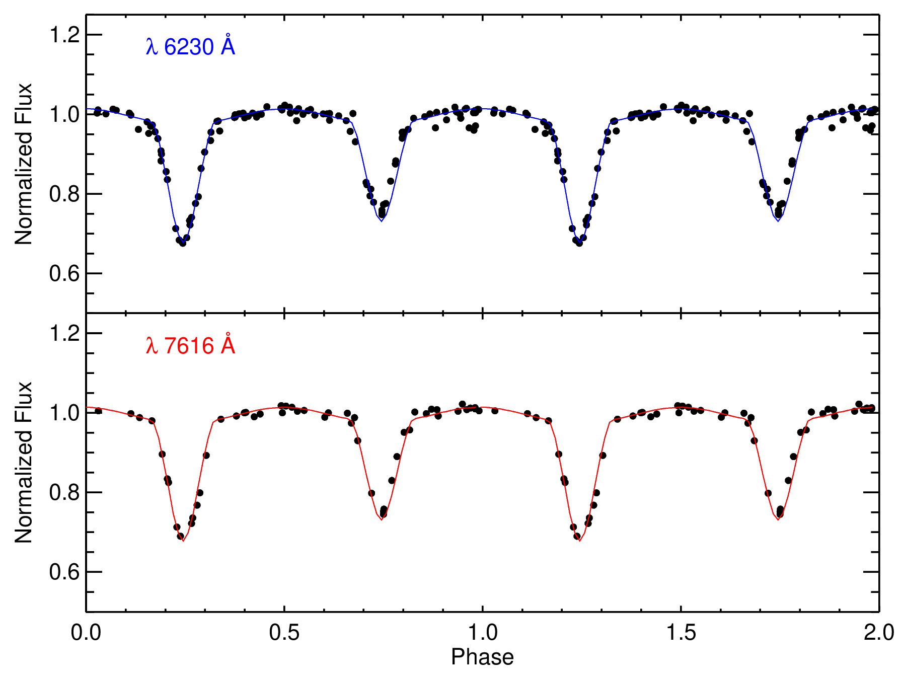
CPD $-$ 59° 2603 or V572 Car (ID:0211 GOSC) is a member of the open cluster Trumpler 16 in the Carina Complex (Rauw et al. 2001). Our PDM analysis yields a period of $2.15285\pm 0.00955642$ days, consistent with the spectroscopic period $2.15294\pm 0.00214$ days obtained by Rauw et al. 2001. A somewhat sparser monitoring of this object was carried out by Antokhin & Cherepashchuk 1993 between 1980-1991. By folding the spectroscopic period with the photometric data obtained by Antokhin & Cherepashchuk 1993, Rauw et al. 2001 derived a lower limit for the inclination ( $i\geq 77^{\circ}$ ) together with the masses for the EB system. This is the first time that a high quality sampled light curve is obtained for this source. We fixed the temperature of the primary star to $T_{1}=35874$ K corresponding to a spectral type O7.5 V (Rauw et al. 2001). The primary component fills up its Roche lobe at $\sim 66\%$ while the secondary at $\sim 75\%$ favouring a detached configuration with an orbital inclination $i=79.2^{\circ}\pm 1.7$ (Fig. 13). The inclination found here is consistent with the lower limit $i\geq 77^{\circ}$ reported by Rauw et al. 2001. We find an effective temperature of $T_{2}=32220$ K for the secondary star corresponding to a spectral type O9.5 V in agreement with the spectroscopic results. Figure. 5 shows the observed light curves in the Sloan $r$ and $i$ filters folded with the orbital period along with the best model.

The results obtained for all the EBs are summarized in Tab. 3; all light curves are displayed in Appendix D along with their best fit model.

4.1 Comparison with previous works

We compare the observed orbital parameters obtained in this work with previous results for high-mass EBs. Those systems are located in the associations Cassiopeia OB6 (Hillwig et al. 2006) and Cygnus OB2 (Kobulnicky et al. 2014, Kiminki et al. 2015), open clusters NGC 6231, in the Scorpious OB1 association (Sana et al. 2003, Sana et al. 2006, Mayer et al. 2017), and Trumpler 16 in the Carina OB1 association (Freyhammer et al. 2001, Niemela et al. 2006). In total there are 15 known periods from previous investigations. Our study yields 47 periods – including the three stars from Paper I. The orbital period distribution covers the range $0.71\leq P\leq 20.14$ days (Fig. 6). Only two objects have orbital periods larger than 10 days (GSC 08173-0018, $P=19.47$ ; Pismis 24-13, $P=20.14$ ) while seven objects exhibit orbital periods shorter than 2 days. The shortest periods are found for TYC 6561-1765-1 and CPD $-$ 24° 2836 with 0.71 and 1.02 days, respectively. Combining our results with the existing values, half of the periods concentrate around 2.4 and 4.8 days. As can be seen in Fig. 6, this bimodal distribution is already apparent in the individual data sets.

Using the rapid binary evolution code from Hurley et al. 2002, Söderhjelm & Dischler 2005 derived the theoretical expected distributions of maximum (primary) eclipse depths ( $\Delta m$ ) versus periods of EBs for different luminosities (their Fig. 8 with $\Delta m>0.1$ mag). In the case of B-type systems, the expected periods range from 0.175 to 65 days. However, for O-type systems no periods shorter than 1.44 days are expected ( $\log P\sim 0.16$ in their Fig. 8 and table A.1). As pointed out by Söderhjelm & Dischler 2005, the mean eclipse probabilities are only valid as long as the systems have similar properties i.e. similar radii, luminosities and orbit sizes. Moreover, their calculations have been carried out by neglecting tidal deformations, reflection effects and assuming zero limb-darkening coefficients. This would explain the fact that in our sample we find three O-type EBs (HD 92607; O9 IV+O9.5 V $P=1.29$ days, ALS 18551; O4.5 V+O4.5 V $P=1.36$ days, and V662 Car; O5 V+O9.5 V $P=1.41$ days) which are near-contact systems with periods shorter than the theoretical limit. CPD -59° 2628 (O9.5 V+O9.5 V) has a slightly larger period ( $P=1.46$ days) than the limit, but has also a near-contact configuration.

All systems from the present survey exhibit circular orbits ( $e=0$ ). This behaviour is a consequence of the short orbital periods because tidal forces will circularize the orbit before Roche lobe overflow (Hurley et al. 2002). A crude estimate of the orbit semi-major axis ( $a$ ) can be obtained from the orbital period by adopting the masses for the effective temperatures and spectral type of the components. We used the masses reported in Martins et al. 2005 for O-type stars and Levenhagen & Leister 2006 and Hohle et al. 2010 for B-type stars. We find a range of $7.52\leq a\leq 70.96\ R_{\odot}$ for B-type systems and $16.13\leq a\leq 122.57\ R_{\odot}$ for O-type systems.

The distribution of mass ratios $q=M_{2}/M_{1}$ is shown in Fig. 7. While the known mass ratios display a fairly uniform distribution between 0.05 and 0.95, the present distribution starts only at $q\sim 0.4$ ; 62% of the systems have mass ratios larger than 0.8. The average value is $q=0.8$ suggesting a large fraction of similar-mass binaries. It is likely that such systems were created during the star formation process rather than by random tidal capture. For instance, the small separation between the components ( $a<1.0$ AU) supports a Kozai cycle star formation scenario (Fabrycky & Tremaine 2007), although a third component could not yet be detected in our sample. One could also speculate that the small separation between the components is an indication for an advanced stage of interaction that could lead to a merger event. This is supported by the large fraction of semi-detached and near-contact systems observed in our sample. On the other hand, semi-detached systems with short periods could be the product of a post-interaction process. Nevertheless we note that the results from the present investigation are biased by the detection method, i.e. transits, which favor compact systems with large diameters of the components. A proper discrimination between different star formation scenarios is only possible after follow-up radial velocity measurements and accurate mass determinations. Fig. 8 corroborates previous results that there is no correlation between mass ratio and orbital period.

5 Conclusions

The current results improve the existing statistics for high-mass EBs significantly. The Roche lobe analysis of 26 systems indicates that 12 systems have a detached geometry while 14 systems have a semi-detached geometry; seven of them are near-contact systems. The high fraction of near-contact systems found in this work suggests that mass transfer will likely dominate their evolution and new contact binary systems will emerge. This agrees with results by Sana et al. 2012 who estimate that more than 70% of high-mass stars will exchange mass with a companion and 30% of them will turn into a binary merger.

Moreover, binary interaction can lead to a significant increase of the stellar rotation rates, and for which, fast rotators will often appear as single stars (de Mink et al. 2011). In that case, if the binary interaction is responsible for the high rotational velocities observed among O-type stars, their multiplicity fraction will be strongly affected. We are engaged in a spectroscopic follow-up study of this sample, in order to investigate the relationship between fast rotation and binary interaction as well as to determine the physical parameters and to track the evolutionary state of the individual systems.

Acknowledgements

We acknowledge support from the IdP II 2015 0002 64 and DIR/WK/2018/09 grants of the Polish Ministry of Science and Higher Education. This research made use of the NASA/IPAC Extragalactic Database (NED) which is operated by the Jet Propulsion Laboratory, California Institute of Technology, under contract with the National Aeronautics and Space Administration. This research has made use of the SIMBAD database, operated at CDS, Strasbourg, France. This research has made use of "Aladin sky atlas" developed at CDS, Strasbourg Observatory, France. We thank the anonymous referee for the constructive comments which contributed to improve this paper.

References

Antokhin & Cherepashchuk (1993) Antokhin, I. I., & Cherepashchuk, A. M. 1993, Astronomy Reports, 37, 152
Antokhin et al. (2008) Antokhin, I. I., Rauw, G., Vreux, J.-M., van der Hucht, K. A., & Brown, J. C. 2008, A&A, 477, 593
Antokhina et al. (2000) Antokhina, E. A., Moffat, A. F. J., Antokhin, I. I., Bertrand, J.-F., & Lamontagne, R. 2000, ApJ, 529, 463
Ardeberg & Maurice (1977) Ardeberg, A., & Maurice, E. 1977, A&AS, 28, 153
Barr Domínguez et al. (2013) Barr Domínguez, A., Chini, R., Pozo Nuñez, F., et al. 2013, A&A, 557, A13
Bate et al. (2002) Bate, M. R., Bonnell, I. A., & Bromm, V. 2002, MNRAS, 336, 705
Baume et al. (1999) Baume, G., Vázquez, R. A., & Feinstein, A. 1999, A&AS, 137, 233
Bertin et al. (2002) Bertin, E., Mellier, Y., Radovich, M., et al. 2002, Astronomical Data Analysis Software and Systems XI, 281, 228
Bertin (2006) Bertin, E. 2006, Astronomical Data Analysis Software and Systems XV, 351, 112
Boch & Fernique (2014) Boch, T., & Fernique, P. 2014, Astronomical Data Analysis Software and Systems XXIII, 485, 277
Boss (2014) Boss, A. P. 2014, American Astronomical Society Meeting Abstracts #223, 223, 214.01
Bonanos (2013) Bonanos, A. Z. 2013, Advancing the Physics of Cosmic Distances, 173
Chini et al. (2012) Chini, R., Hoffmeister, V. H., Nasseri, A., Stahl, O., & Zinnecker, H. 2012, MNRAS, 424, 1925
Chini et al. (2013) Chini, R., Barr, A., Buda, L. S., et al. 2013, Central European Astrophysical Bulletin, 37, 295
Crowther et al. (2006) Crowther, P. A., Hadfield, L. J., Clark, J. S., Negueruela, I., & Vacca, W. D. 2006, MNRAS, 372, 1407
Dachs et al. (1982) Dachs, J., Kaiser, D., Sherwood, W. A., & Nikolov, A. 1982, A&AS, 50, 261
Delgado-Donate et al. (2004) Delgado-Donate, E. J., Clarke, C. J., Bate, M. R., et al. 2004, MNRAS, 351, 617
de Mink et al. (2011) de Mink, S. E., Langer, N., & Izzard, R. G. 2011, Active OB Stars: Structure, Evolution, Mass Loss, and Critical Limits, 272, 531
de Mink et al. (2014) de Mink, S. E., Sana, H., Langer, N., Izzard, R. G., & Schneider, F. R. N. 2014, ApJ, 782, 7
De Rosa et al. (2014) De Rosa, R. J., Patience, J., Wilson, P. A., et al. 2014, MNRAS, 437, 1216
Denoyelle (1977) Denoyelle, J. 1977, A&AS, 27, 343
Diaz-Cordoves & Gimenez (1992) Diaz-Cordoves, J., & Gimenez, A. 1992, A&A, 259, 227
Drake et al. (2014) Drake, A. J., Djorgovski, S. G., García-Álvarez, D., et al. 2014, ApJ, 790, 157
Drilling (1968) Drilling, J. S. 1968, AJ, 73, 590
Drilling (1991) Drilling, J. S. 1991, ApJS, 76, 1033
Duchêne & Kraus (2013) Duchêne, G., & Kraus, A. 2013, ARA&A, 51, 269
Dunstall et al. (2015) Dunstall, P. R., Dufton, P. L., Sana, H., et al. 2015, A&A, 580, A93
Fabrycky & Tremaine (2007) Fabrycky, D., & Tremaine, S. 2007, ApJ, 669, 1298
Fang et al. (2012) Fang, M., van Boekel, R., King, R. R., et al. 2012, A&A, 539, A119
Feinstein (1963) Feinstein, A. 1963, PASP, 75, 492
Feinstein (1969) Feinstein, A. 1969, MNRAS, 143, 273
Feinstein & Vazquez (1989) Feinstein, A., & Vazquez, R. A. 1989, A&AS, 77, 321
Fitzgerald (1970) Fitzgerald, M. P. 1970, A&A, 4, 234
Fitzgerald (1987) Fitzgerald, M. P. 1987, MNRAS, 229, 227
Forte (1976) Forte, J. C. 1976, A&AS, 25, 271
Freyhammer et al. (2001) Freyhammer, L. M., Clausen, J. V., Arentoft, T., & Sterken, C. 2001, A&A, 369, 561
Fruth et al. (2012) Fruth, T., Kabath, P., Cabrera, J., et al. 2012, AJ, 143, 140
Fuhrmann & Chini (2012) Fuhrmann, K., & Chini, R. 2012, ApJS, 203, 30
Fuhrmann et al. (2017) Fuhrmann, K., Chini, R., Kaderhandt, L., & Chen, Z. 2017, ApJ, 836, 139
Gaia Collaboration (2018) Gaia Collaboration 2018, VizieR Online Data Catalog, 1345,
Gies et al. (2002) Gies, D. R., Penny, L. R., Mayer, P., Drechsel, H., & Lorenz, R. 2002, ApJ, 574, 957
Goodwin & Kroupa (2005) Goodwin, S. P., & Kroupa, P. 2005, A&A, 439, 565
Halbwachs et al. (2003) Halbwachs, J. L., Mayor, M., Udry, S., & Arenou, F. 2003, A&A, 397, 159
Hackstein et al. (2015) Hackstein, M., Fein, C., Haas, M., et al. 2015, Astronomische Nachrichten, 336, 590
Havlen (1972) Havlen, R. J. 1972, A&A, 17, 413
Heske & Wendker (1984) Heske, A., & Wendker, H. J. 1984, A&AS, 57, 205
Hillwig et al. (2006) Hillwig, T. C., Gies, D. R., Bagnuolo, W. G., Jr., et al. 2006, ApJ, 639, 1069
Hiltner & Johnson (1956) Hiltner, W. A., & Johnson, H. L. 1956, ApJ, 124, 367
Hohle et al. (2010) Hohle, M. M., Neuhäuser, R., & Schutz, B. F. 2010, Astronomische Nachrichten, 331, 349
Høg et al. (2000) Høg, E., Fabricius, C., Makarov, V. V., et al. 2000, A&A, 355, L27
Hur et al. (2012) Hur, H., Sung, H., & Bessell, M. S. 2012, AJ, 143, 41
Hurley et al. (2002) Hurley, J. R., Tout, C. A., & Pols, O. R. 2002, MNRAS, 329, 897
Kaderhandt et al. (2015) Kaderhandt, L., Barr Domínguez, A., Chini, R., et al. 2015, Astronomische Nachrichten, 336, 677
Kiminki et al. (2015) Kiminki, D. C., Kobulnicky, H. A., Vargas Álvarez, C. A., Alexander, M. J., & Lundquist, M. J. 2015, ApJ, 811, 85
Kobulnicky et al. (2014) Kobulnicky, H. A., Kiminki, D. C., Lundquist, M. J., et al. 2014, ApJS, 213, 34
Kozai (1962) Kozai, Y. 1962, AJ, 67, 591
Krumholz et al. (2007) Krumholz, M. R., Klein, R. I., & McKee, C. F. 2007, ApJ, 656, 959
Lafler & Kinman (1965) Lafler, J., & Kinman, T. D. 1965, ApJS, 11, 216
Landolt (1983) Landolt, A. U. 1983, AJ, 88, 439
Landolt (2009) Landolt, A. U. 2009, AJ, 137, 4186
Leahy & Leahy (2015) Leahy, D. A., & Leahy, J. C. 2015, Computational Astrophysics and Cosmology, 2, 4
Levenhagen & Leister (2006) Levenhagen, R. S., & Leister, N. V. 2006, MNRAS, 371, 252
Lodén (1966) Lodén, L. O. 1966, Arkiv for Astronomi, 4, 65
Lyngå (1969) Lyngå, G. 1969, Arkiv for Astronomi, 5, 181
McSwain et al. (2007) McSwain, M. V., Boyajian, T. S., Grundstrom, E. D., & Gies, D. R. 2007, ApJ, 655, 473
Maíz Apellániz et al. (2016) Maíz Apellániz, J., Sota, A., Arias, J. I., et al. 2016, ApJS, 224, 4
Martins et al. (2005) Martins, F., Schaerer, D., & Hillier, D. J. 2005, A&A, 436, 1049
Mayer et al. (2017) Mayer, P., Harmanec, P., Chini, R., et al. 2017, A&A, 600, A33
Massey & Johnson (1993) Massey, P., & Johnson, J. 1993, AJ, 105, 980
Massey et al. (2001) Massey, P., DeGioia-Eastwood, K., & Waterhouse, E. 2001, AJ, 121, 1050
Moffat & Vogt (1973) Moffat, A. F. J., & Vogt, N. 1973, A&AS, 10, 135
Moffat et al. (1977) Moffat, A. F. J., Fitzgerald, M. P., & Jackson, P. D. 1977, ApJ, 215, 106
Muzzio & Orsatti (1977) Muzzio, J. C., & Orsatti, A. M. 1977, AJ, 82, 474
Muzzio (1979) Muzzio, J. C. 1979, AJ, 84, 639
Nassau & Stephenson (1963) Nassau, J. J., & Stephenson, C. B. 1963, Hamburger Sternw. Warner & Swasey Obs.,
Nazé et al. (2005) Nazé, Y., Antokhin, I. I., Sana, H., Gosset, E., & Rauw, G. 2005, MNRAS, 359, 688
Neckel (1984) Neckel, T. 1984, A&A, 137, 58
Niemela et al. (2006) Niemela, V. S., Morrell, N. I., Fernández Lajús, E., et al. 2006, MNRAS, 367, 1450
Nordström (1975) Nordström, B. 1975, A&AS, 21, 193
Orsatti (1992) Orsatti, A. M. 1992, AJ, 104, 590
Peton-Jonas (1981) Peton-Jonas, D. 1981, A&AS, 45, 193
Pojmanski (2003) Pojmanski, G. 2003, Acta Astron., 53, 341
Povich et al. (2009) Povich, M. S., Churchwell, E., Bieging, J. H., et al. 2009, ApJ, 696, 1278
Rauw et al. (2001) Rauw, G., Sana, H., Antokhin, I. I., et al. 2001, MNRAS, 326, 1149
Reed & Fitzgerald (1983) Reed, B. C., & Fitzgerald, M. P. 1983, MNRAS, 205, 241
Reed (1990) Reed, B. C. 1990, AJ, 100, 737
Reed & Vance (1996) Reed, B. C., & Vance, S. J. 1996, AJ, 112, 2855
Reed (2003) Reed, B. C. 2003, AJ, 125, 2531
Reed (2005) Reed, B. C. 2005, AJ, 130, 1652
Rucinski (1992) Rucinski, S. M. 1992, AJ, 103, 960
Russeil et al. (2012) Russeil, D., Zavagno, A., Adami, C., et al. 2012, A&A, 538, A142
Sana et al. (2003) Sana, H., Hensberge, H., Rauw, G., & Gosset, E. 2003, A&A, 405, 1063
Sana et al. (2006) Sana, H., Gosset, E., & Rauw, G. 2006, MNRAS, 371, 67
Sana et al. (2008) Sana, H., Nazé, Y., O’Donnell, B., Rauw, G., & Gosset, E. 2008, New Astron., 13, 202
Sana et al. (2012) Sana, H., de Mink, S. E., de Koter, A., et al. 2012, Science, 337, 444
Sana et al. (2013) Sana, H., Le Bouquin, J.-B., Mahy, L., et al. 2013, A&A, 553, A131
Scargle (1982) Scargle, J. D. 1982, ApJ, 263, 835
Schild et al. (1983) Schild, R. E., Garrison, R. F., & Hiltner, W. A. 1983, ApJS, 51, 321
Schöller et al. (2012) Schöller, M., Correia, S., Hubrig, S., & Ageorges, N. 2012, Progress in Solar/Stellar Physics with Helio- and Asteroseismology, 462, 87
Schwarzenberg-Czerny (1999) Schwarzenberg-Czerny, A. 1999, ApJ, 516, 315
Slawson & Reed (1988) Slawson, R. W., & Reed, B. C. 1988, J. R. Astron. Soc. Canada, 82, 276
Söderhjelm & Dischler (2005) Söderhjelm, S., & Dischler, J. 2005, A&A, 442, 1003
Söderhjelm (2007) Söderhjelm, S. 2007, A&A, 463, 683
Sota et al. (2014) Sota, A., Maíz Apellániz, J., Morrell, N. I., et al. 2014, ApJS, 211, 10
Stephenson & Hobbs (1961) Stephenson, C. B., & Hobbs, R. W. 1961, AJ, 66, 186
Stephenson & Sanduleak (1971) Stephenson, C. B., & Sanduleak, N. 1971, Publications of the Warner & Swasey Observatory, 1,
Stephenson & Sanduleak (1977) Stephenson, C. B., & Sanduleak, N. 1977, ApJS, 33, 459
Stellingwerf (1978) Stellingwerf, R. F. 1978, ApJ, 224, 953
Stetson (1996) Stetson, P. B. 1996, PASP, 108, 851
Sterzik et al. (2003) Sterzik, M. F., Durisen, R. H., & Zinnecker, H. 2003, A&A, 411, 91
Sundman et al. (1974) Sundman, A., Loden, L. O., & Nordström, B. 1974, A&AS, 16, 445
Sung et al. (1998) Sung, H., Bessell, M. S., & Lee, S.-W. 1998, AJ, 115, 734
Theodossiou & Danezis (1991) Theodossiou, E., & Danezis, E. 1991, Ap&SS, 183, 91
Tokovinin (2008) Tokovinin, A. 2008, MNRAS, 389, 925
van Hamme (1993) van Hamme, W. 1993, AJ, 106, 2096
Vazquez et al. (1996) Vazquez, R. A., Baume, G., Feinstein, A., & Prado, P. 1996, A&AS, 116, 75
Vijapurkar & Drilling (1993) Vijapurkar, J., & Drilling, J. S. 1993, ApJS, 89, 293
Walborn (1987) Walborn, N. R. 1987, AJ, 93, 868
Wang et al. (2007) Wang, J., Townsley, L. K., Feigelson, E. D., et al. 2007, ApJS, 168, 100
Wenger et al. (2000) Wenger, M., Ochsenbein, F., Egret, D., et al. 2000, A&AS, 143, 9
Westerlund & Garnier (1989) Westerlund, B. E., & Garnier, R. 1989, A&AS, 78, 203
Wilson & Devinney (1971) Wilson, R. E., & Devinney, E. J. 1971, ApJ, 166, 605
Wilson (1979) Wilson, R. E. 1979, ApJ, 234, 1054
Wilson (1990) Wilson, R. E. 1990, ApJ, 356, 613
Wramdemark (1976) Wramdemark, S. 1976, A&AS, 23, 231
Zacharias et al. (2013) Zacharias, N., Finch, C. T., Girard, T. M., et al. 2013, AJ, 145, 44
Zinnecker (2003) Zinnecker, H. 2003, A Massive Star Odyssey: From Main Sequence to Supernova, 212, 80

Appendix A The performance of the PDM algorithm and the time span of the monitoring campaign

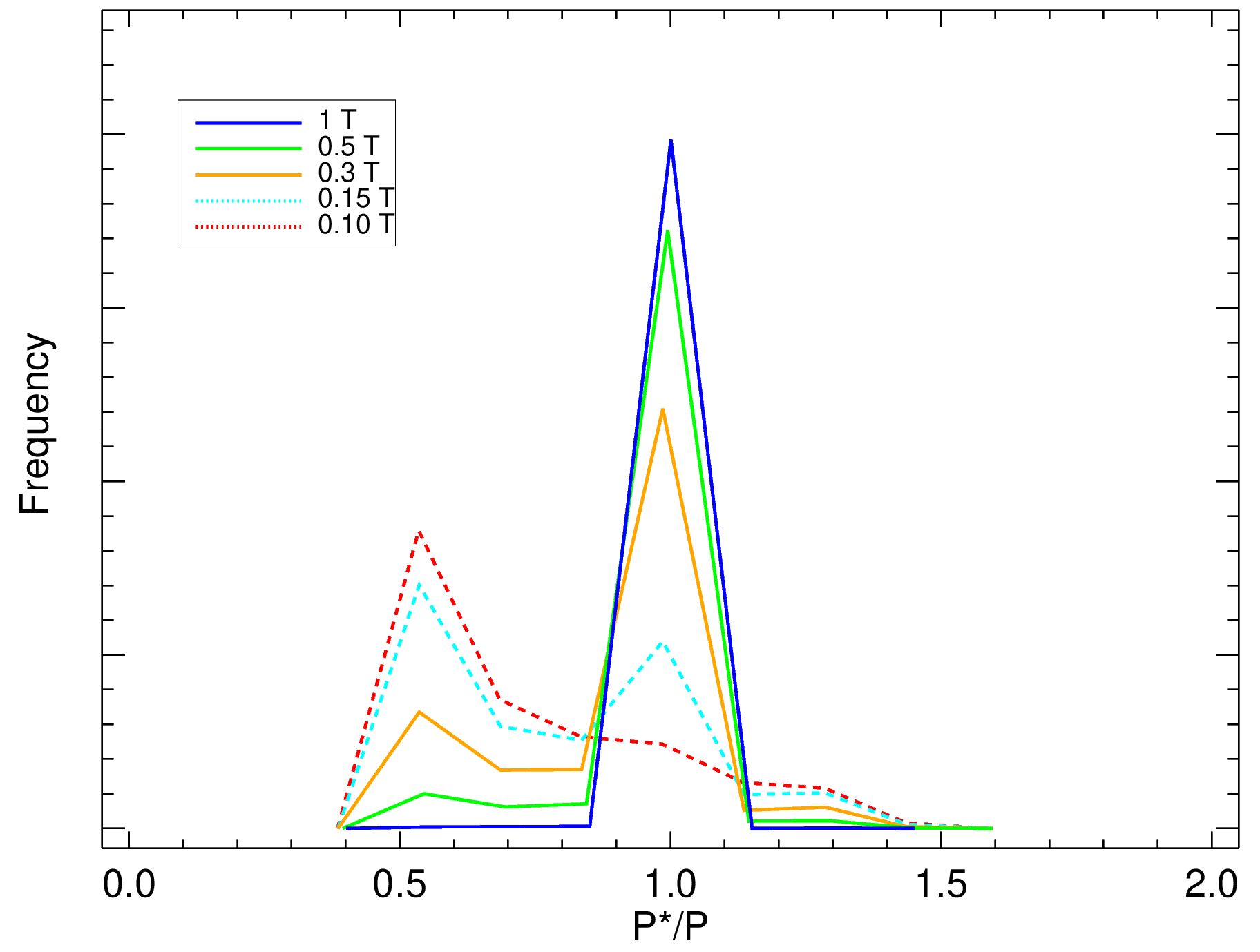
In order to test the efficiency of the PDM algorithm, and to identify potential biases with respect to the true period, we create 2000 randomly sampled light curves with different number of observations $T$ for the EBs CPD $-$ 59° 2603. We use the sloan $r$ light curve with a total of 109 data points and which yields a period $P=2.152851\pm 0.009556$ as determined in section 4. For each of the 2000 light curves, we calculate the period $P*$ using the PDM algorithm. The recovered $P*$ distributions are shown in Figure 10. We find that the algorithm performs reliable even when using only $\sim 30\%$ of the original data points (brown solid line). The centroid of the distributions are clearly biased to shorter periods if the amount of observations decrease to $\sim 15\%$ (magenta dotted line), although still the algorithm is able to recover the true period in about $40\%$ of the cases. The extreme situation can be seen if the amount of observations decrease by $\sim 90\%$ . For that case, the distribution is biased to almost half of the true period $P$ . As already mentioned in Paper 1, the reliability of the PDM to work with only a moderate number of data points is a crucial advantage over other algorithms that strongly depends on the amount of observations (e.g. Lomb-Scargle periodogram by Scargle 1982, analysis of variance by Schwarzenberg-Czerny 1999).

Appendix B Individual sources with EBs models

In the following, we discuss the multiple high-mass systems in more detail and describe their properties as obtained from the light curve analysis.

B.1 CPD $-$ 24° 2836

CPD $-$ 24° 2836 (CD $-$ 24° 5918, TYC 6544-559-1) was catalogued as O9-B0 by Nordström 1975 with the remark that the spectrum was "disturbed by overlap". The blue magnitude is given as $B=11.3$ . The Tycho-2 catalog (Høg et al. 2000) give photometric values $B=11.25$ and $V=11.17$ , while our photometry yields $B=11.40$ and $V=11.28$ . These differences might indicate a faint color variability. Our $UBV$ values yield a photometric spectral type of B7 V, significantly later than the classification from the objective prism observation. This large deviation may be due to both photometric errors and/or the indicated color variability. Additionally, a secondary of lower mass may enhance this effect. We therefore trust the spectroscopic classification and adopt a spectral type of B0 V with an effective temperature of $T_{1}=29230$ K.

The system shows well-defined eclipses favouring a detached configuration with an inclination $i=57.3^{\circ}$ where both components fill up their Roche lobes at about 86% and 83% (Fig. 11). The temperature of the secondary component is $T_{2}=19520$ K compatible with a spectral type B2.5 V.

B.2 CPD $-$ 26° 2656

The star CPD $-$ 26° 2656 (CD $-$ 26° 5070, TYC 6561-87-1) was classified as a double-lined binary (B1: V:) by Lodén 1966 displaying photometric variability; the quoted photometry is $U=10.64$ , $B=11.28$ , and $V=11.0$ . The star is also contained in the spectral survey of the Southern Milky Way (Nordström 1975) and listed there as No. 79; the blue magnitude is $B=11.2$ and the spectral classification is OB:. Peton-Jonas 1981 give a tentative spectral classification of B0 V based on the strength of H $\gamma$ and H $\delta$ . Eventually, Reed & Fitzgerald 1983 list the star as B5 V; the quoted photometry is $U=10.57$ , $B=11.18$ , and $V=10.95$ . Our own photometry yields $U=10.55$ , $B=11.18$ , and $V=10.95$ in agreement with the previous values and suggests a photometric spectral type of B1 V. Summarizing the spectroscopic results we prefer a B1-type star which agrees perfectly with its dereddened $UBV$ colors (Fig. 3). We therefore fixed the effective temperature of the primary star to $T_{1}=25570$ K.

The eclipsing nature of CPD $-$ 26° 2656 was already established by Pojmanski 2003 using data from the All Sky Automated Survey (ASAS II) catalogue of variable stars. The author determined a photometric period of $2.6990$ days and suggested a detached EB configuration; we obtain the same period. The light curves in both filters show similar variations with the primary and secondary minimum having different depths $\Delta D_{p}=\Delta D_{p,min}-\Delta D_{max}=33\%$ and $\Delta D_{s}=\Delta D_{s,min}-\Delta D_{max}=28\%$ . This can be interpreted by a temperature difference of the components. The model fit of the light curve yields an effective temperature of $T_{2}=23250$ K for the secondary component corresponding to a spectral type of about B2 V.

The primary component fills up its Roche lobe at $\sim 65\%$ while the secondary at $\sim 74\%$ favouring a detached configuration with an orbital inclination $i=79.7^{\circ}$ (Fig. 11).

B.3 TYC 6561-1765-1

TYC 6561-1765-1 was classified as O9.5 V: by Peton-Jonas 1981, their No. 1469; however, this designation was regarded as doubtful by the authors. The Tycho-2 catalog (Høg et al. 2000) give photometric values $B=12.30$ and $V=11.97$ . Our own photometry yields $B=12.52$ and $V=12.30$ suggesting some variability. Including our $U$ -value of 12.13 we obtain a photometric classification of B3 V. The photometric agreement with the Tycho-2 catalog leads us to fix the effective temperature of the primary star to $T_{1}=18445$ K.

The light curves in both filters show similar variations with amplitudes $\Delta D_{p}=6\%$ and $\Delta D_{s}=5\%$ for the primary and secondary minimum respectively. The primary component fills up its Roche lobe at $\sim 88\%$ while the secondary at $\sim 71\%$ favouring a detached configuration with an orbital inclination $i=55.7^{\circ}$ (Fig. 11). The model fit of the light curve yields an effective temperature of $T_{2}=13150$ K for the secondary component corresponding to a spectral type of about B7 V.

B.4 CD $-$ 31° 5524

The star CD $-$ 31° 5524 was originally classified as O9-9.5 by Nordström 1975, their No. 163. Orsatti 1992 provided $UBV$ photometry with $V=11.37$ and colors $B-V=0.26$ and $U-B=-0.52$ . Subsequent observations performed by Reed 1990 yield consistent photometric results with $V=11.40$ and colors $B-V=0.27$ and $U-B=-0.59$ ; the colors are compatible with a reddened B1 V. star (Fig. 3). We therefore fixed the effective temperature of the primary star to $T_{1}=25570$ K. The primary and secondary components fill up their Roche lobes to about 97% and 95%, respectively, favouring a near-contact configuration with an orbital inclination of $i=53.2^{\circ}$ . The 3D view of the Roche geometry of the system ( $\phi=0.54$ ) shows that most likely the future mass transfer will create a new contact binary system (Fig. 11).

B.5 CPD $-$ 42° 2880

Objective prism spectra of CPD $-$ 42° 2880 (TYC 7687-444-1, LS 1142) yield the classification O9.5-B2 (Nordström 1975), their No. 300, with a blue magnitude of $B=11.7$ . The Tycho-2 catalog (Høg et al. 2000) give photometric values $B=11.70$ and $V=11.17$ while Denoyelle 1977 give $U=11.53$ , $B=11.80$ , and $V=11.10$ . Our own photometry yields $U=11.53$ , $B=11.80$ , and $V=11.10$ in perfect accord with the previous values and suggests a photometric spectral type of B0 V. This agreement with the classification from the objective prism spectrum leads us to fix the effective temperature of the primary star to $T_{1}=29230$ K.

The system shows well-defined eclipses favouring a detached configuration, where both components fill up their Roche lobes at about 73% and 72%, respectively. The temperature of the secondary component is $T_{2}=22110$ K equivalent to a B2 V. As displayed in Fig. 11, the light curves show nearly identical amplitude variations with primary and secondary minimum eclipses at different depths ( $\Delta D_{p}=8\%$ , $\Delta D_{s}=6\%$ ). This behaviour is characteristic for an eclipsing binary with different effective temperatures; the primary minimum is due to the eclipse of the more luminous star by the less luminous companion. The primary and secondary minima are separated symmetrically by 0.6 in phase suggesting a circular orbit.

B.6 CPD $-$ 45° 3253

CPD $-$ 45° 3253 (CD $-$ 45° 4706, TYC 8152-206-1, LS 1207) was classified as B0: by Nordström 1975, their No. 373; the blue magnitude is listed as $B=12.0$ . This object is part of a survey searching for faint OB stars in the Vela region (Muzzio & Orsatti 1977). These authors derive a spectral designation of OB⁰, their star No. 36, and obtain photometric values of $B=12.01$ and $V=10.77$ . Slawson & Reed 1988 derive a spectral type of O9:, also based on objective-prism spectroscopy; furthermore they list photometric values of $B=11.99$ and $V=10.79$ . The Tycho-2 catalog (Høg et al. 2000) give photometric values $B=11.54$ and $V=10.62$ . Our own photometry yields $B=11.97$ and $V=10.88$ suggesting some variability. Including our $U$ -value of 12.31 we obtain a photometric classification of B3 V. As an average we fix the effective temperature of the primary star to $T_{1}=29230$ K, corresponding to a B0 V star.

The primary and secondary minimum eclipses are separated symmetrically by 0.11 in phase at depths of $\Delta D_{p}=9\%$ and $\Delta D_{s}=6\%$ . The best-fitting model favours a detached configuration with an inclination $i=64.1^{\circ}$ and requires that both components fill up their Roche lobes at about 73% and 72%, respectively (Fig. 12). Our calculations yield an effective temperature of $T_{2}=22250$ K for the secondary star suggesting that this new system is most likely composed of B0 V + B2 V.

B.7 GSC 08156-03066

GSC 08156-03066 is part of the survey of faint OB stars performed by Muzzio & Orsatti 1977, their star No. 4; the authors derived a spectral designation of OB⁰ and obtained photometric values of $B=13.16$ and $V=11.79$ . Muzzio & Orsatti 1977 provided $UBV$ photometry with $U=13.26$ , $B=13.01$ , and $V=11.78$ which is compatible with the previous values and suggests a photometric spectral type of B1 V. Our own photometry yields $U=13.32$ , $B=13.18$ , and $V=11.93$ indicating a spectral type of O9.5, slightly earlier than the classification by Muzzio & Orsatti 1977. While our $B-V$ color is consistent with the result obtained by Muzzio & Orsatti 1977, the $U-B$ color differs by 0.11 mag. We therefore prefer a spectral type B1 V with an effective temperature $T_{1}=25570$ K.

The system shows well-defined eclipses with a period of 2.3318 days. The amplitude variations for the primary and secondary minimum are $\Delta D_{p}=10\%$ and $\Delta D_{s}=9\%$ suggesting similar temperatures for both components. The temperature of the secondary component is $T_{2}=24150$ K suggesting a pair of two B1 V stars. As displayed in Fig. 12, the 3D view of the Roche geometry at phase $\phi=0.50$ shows that the system has a semi-detached geometry where both stars are close to filling their Roche lobes.

B.8 GSC 08173-00182

GSC 08173-00182 is also located in the Vela region. Muzzio & Orsatti 1977 give a classification of OB⁺ but claim it as doubtful (their No. 101). The photometric entries for this star are $B=14.24$ and $V=12.55$ . Our own photometry yields $B=14.40$ and $V=12.79$ suggesting some variability. Including our $U$ -value of 15.24 we obtain a photometric classification of B5 V. Taking into account that main sequence stars from the OB⁺ group tend to be of earlier spectral type we adopt a B3 V classification for the primary. This leaves us with an effective primary temperature of $T_{1}=18445$ K.

The primary and secondary minimum eclipses are separated symmetrically by 0.15 in phase. The model suggests a detached system (Fig. 12). The temperature of the secondary component is $T_{2}=13920$ K suggesting that this new system is most likely composed of B3 V + B6 V.

B.9 TYC 8175-685-1

The star TYC 8175-685-1 (ALS 17580) was classified as OB^- by Muzzio & Orsatti 1977, their No. 143; however, this designation was regarded as doubtful by the authors. The photometric values are $B=13.35$ and $V=12.24$ . Muzzio (1979) provided $UBV$ photometry with $U=13.55$ , $B=13.23$ , and $V=12.10$ which is compatible with the previous values. In the following we adopt a photometric spectral type of B3 V and fix the effective temperature to $T_{1}=18445$ K for the primary.

Using data from the ASAS II archive Pojmanski 2003 determined a photometric period of $3.4085$ days. Furthermore, he suggested that TYC 8175-685-1 forms an eclipsing contact (or almost contact) binary configuration. We obtain the identical photometric period as reported by Pojmanski 2003. The amplitude variations for the primary and secondary minimum eclipses are $\Delta D_{p}=14\%$ and $\Delta D_{s}=13\%$ , respectively, suggesting again similar temperatures for both components. This yields a B3 V + B3 V system.

As displayed in Fig. 12, the 3D view of the Roche geometry of the system ( $\phi=0.54$ ) shows that the system has a semi-detached (near-contact) geometry where both stars are close to filling their Roche lobes. Most likely the future mass transfer will create a new contact binary system.

B.10 ALS 18551

ALS 18551 is a member of the open cluster Collinder 228 and was originally classified as an O5 star by Wramdemark 1976 using photometric data. We notice that the ALS 18551 identification in SIMBAD (Wenger et al. 2000) is based on a relatively large distance to the given source ( $\sim$ 10.8"). The Website displays an image centred on the corresponding source coordinates based on Aladin Lite (Boch & Fernique 2014) which shows no recognizable object at the given position. Manual inspection of our coordinates shows a matching object in Aladin Lite. The SIMBAD coordinate is referenced by Wramdemark 1976. Therein, the object matches (epoch B1950) and the given plate image shows the correct source.

High-resolution spectroscopy (Maíz Apellániz et al. 2016) has detected a O4.5 V SB2 spectroscopic binary; however, no period has been published to date. From our light curves we obtain a photometric period of 1.360 days. We fixed $T_{1}=41860$ K according to the spectral type reported by Maíz Apellániz et al. 2016 and used the observational $T_{\rm eff}$ calibration by Martins et al. 2005 (his Table 4). The system shows well-defined eclipses favouring a near-contact configuration, where both components fill up their Roche lobes at about 93% and 92%, respectively (Fig. 12). The model fit of the light curve yields an effective temperature of the secondary star $T_{2}=41460$ K which is consistent with the spectroscopic results obtained by Maíz Apellániz et al. 2016. Here we confirm photometrically that the system is composed of two O4.5 V stars.

B.11 CPD $-$ 39° 7292

The star CPD $-$ 39° 7292 was first observed by Dachs et al. 1982 as part of a monitoring of luminous stars in the southern Milky Way. The reported photometric values are $U=11.33$ , $B=11.53$ , and $V=10.81$ ; the colors are compatible with a reddened B1 V (Fig. 3). Drilling (1991) give a classification of OB⁺ and provided $UBV$ photometry with $U=11.51$ , $B=11.74$ , and $V=10.96$ ; the colors are compatible with a reddened B0 V star (Fig. 3). Subsequent spectroscopic observations by Vijapurkar & Drilling 1993 yielded a spectral type B1 III n. Our own photometry yields $U=11.59$ , $B=11.88$ , and $V=11.01$ corresponding to a spectral type O5, significantly earlier than the spectroscopic and past photometric observations. Moreover, the three different photometric data sets indicate a color variability and therefore we prefer to adopt a spectral type B0V with an effective temperature of $T_{1}=25570$ K. The assumed spectral type is consistent with both previous photometric results (Dachs et al. 1982; Drilling 1991) and the spectroscopic results by Vijapurkar & Drilling 1993.

The amplitude variations for the primary and secondary minimum eclipses are $\Delta D_{p}=15\%$ and $\Delta D_{s}=10\%$ , which can be interpreted through the difference between the temperatures of the components. The primary and secondary components fills up their Roche lobe about 98% and 99% respectively, favouring a near-contact configuration with an orbital inclination of $i=52.5^{\circ}$ . The 3D view of the Roche geometry of the system ( $\phi=0.50$ ) shows that most likely future mass transfer will create a new contact binary system (Fig. 13).

B.12 Pismis 24-4

The star Pismis 24-4 belongs to the young open cluster Pismis 24 which resides within NGC 6357 in the Sagittarius spiral arm at a distance of 1.7 kpc (Fang et al. 2012). This well-studied region is known as a rich reservoir of young stars, containing several OB stars (Massey et al. 2001) and several shell-like H ii regions (Russeil et al. 2012).

Pismis 24-4 was classified as a O9-B0? by Wang et al. 2007; this tentative spectral type was inferred from a color-magnitude diagram by dereddening 2MASS colors to the 1 Myr pre-main sequence (pre-MS) isochrone. Moffat & Vogt 1973 presented the original $UBV$ photometry with $U=15.89$ , $B=15.36$ , and $V=13.93$ ; these colors are compatible with a reddened B3 V star. In the following we adopt a spectral type B0 V and fix the effective temperature of the primary to $T_{1}=29230$ K.

The light curves show that the primary and secondary minimum have the same amplitude variations ( $\sim 14\%$ ), characteristic for an eclipsing binary with equal effective temperatures. We therefore suggest that this new system is most likely composed of two B0 V stars. The primary component fills up its Roche lobe about 76% while the secondary about 96% favouring a semi-detached configuration with an orbital inclination of 61.9^∘. As displayed in Fig. 13, the 3D view of the Roche geometry of the system, $\phi=0.88$ shows a transitional evolutionary state of the system for which one of the stars is close to fill its Roche lobe.

B.13 CD $-$ 29° 14032

CD $-$ 29° 14032 was classified as B1 III by Vijapurkar & Drilling 1993. The Tycho-2 catalog (Høg et al. 2000) give photometric values $B=11.72$ and $V=11.96$ . Our own photometry yields $B=11.69$ and $V=11.05$ which suggest variability. Including our $U-$ value of 11.30 we obtain a photometric classification of O9.5 V. As an average we fix the effective temperature of the primary star to $T_{1}=29230$ K, corresponding to a B0 V star.

The system shows well-defined eclipses favouring a detached configuration (Fig. 13), where both components fill up their Roche lobes at about 76% and 73%, respectively. The best fit to the light curve yields a temperature of $T_{2}=26850$ K for the secondary component corresponding to a spectral type B1 V.

B.14 CPD $-$ 59° 2603

CPD $-$ 59° 2603 or V572 Car (ID:0211 GOSC) is a member of the open cluster Trumpler 16 in the Carina Complex (Rauw et al. 2001). We find a period of $2.152851\pm 0.009556$ days consistent with the spectroscopic period $2.15294\pm 0.00214$ days obtained by Rauw et al. 2001. A somewhat sparser monitoring of this object was carried out by Antokhin & Cherepashchuk 1993 between 1980-1991. By folding the spectroscopic period with the photometric data obtained by Antokhin & Cherepashchuk 1993, Rauw et al. 2001 derived a lower limit for the inclination ( $i\geq 77^{\circ}$ ) together with the masses for the EB system. This is the first time that a high quality sampled light curve is obtained for this source. We fixed the temperature of the primary star to $T_{1}=35874$ K corresponding to a spectral type O7.5 V (Rauw et al. 2001). The primary component fills up its Roche lobe at $\sim 66\%$ while the secondary at $\sim 75\%$ favouring a detached configuration with an orbital inclination $i=79.2^{\circ}\pm 1.7$ (Fig. 13). The inclination found here is consistent with the lower limit $i\geq 77^{\circ}$ reported by Rauw et al. 2001. We find an effective temperature of $T_{2}=32220$ K for the secondary star corresponding to a spectral type O9.5 V in agreement with the spectroscopic results.

B.15 CPD $-$ 59° 2628

CPD $-$ 59° 2628 has been catalogued by GOSC (ID:0218) with a spectral type of O9.5 V. Therefore, we fixed the temperature of the primary star to $T_{1}=31884$ K. The system shows well-defined eclipses with a period of $1.46\pm 0.015$ days as derived with the PDM algorithm. The amplitude variations for the primary and secondary minimum are $\Delta D_{p}=38\%$ and $\Delta D_{s}=34\%$ suggesting slightly different temperatures for both components. The primary component fills up its Roche lobe at $\sim 96\%$ , the secondary at $\sim 95\%$ favouring a near-contact configuration with an orbital inclination $i=73.4^{\circ}$ . We find an effective temperature of $T_{2}=30120$ K for the secondary star corresponding to a spectral type O9.5 V.

B.16 CPD $-$ 59° 2635

The GOSC (ID:0220) gives a spectral type O8 V; therefore we fixed the temperature of the primary star to $T_{1}=34877$ K. The primary component fills up its Roche lobe at $\sim 78\%$ , the secondary at $\sim 69\%$ favouring a detached configuration with an orbital inclination $i=75.2^{\circ}$ (Fig. 13). We find an effective temperature of $T_{2}=31090$ K for the secondary star corresponding to a spectral type O9.5 V.

B.17 V662 Car

The GOSC (ID:0226) gives a spectral type O5 V; therefore we fixed the temperature of the primary star to $T_{1}=40862$ K. The primary component fills up its Roche lobe at $\sim 96\%$ , the secondary at $\sim 95\%$ favouring a near-contact configuration with an orbital inclination $i=74.3^{\circ}$ (Fig. 13). We find an effective temperature of $T_{2}=31989$ K for the secondary star corresponding to a spectral type O9.5 V.

B.18 TYC 7370-460-1

The GOSC (ID:0375) gives a spectral type O6 V; therefore we fixed the temperature of the primary star to $T_{1}=38867$ K. The primary component fills up its Roche lobe at $\sim 82\%$ , the secondary at $\sim 79\%$ favouring a detached configuration with an orbital inclination $i=80.3^{\circ}$ (Fig. 13). We find an effective temperature of $T_{2}=32120$ K for the secondary star corresponding to a spectral type O9 V.

B.19 Pismis 24-13

The GOSC (ID:0398) gives a spectral type O6 V; therefore we fixed the temperature of the primary star to $T_{1}=38867$ K. The primary component fills up its Roche lobe at $\sim 91\%$ , the secondary at $\sim 91\%$ favouring a semi-detached configuration (near contact) with an orbital inclination $i=51.9^{\circ}$ (Fig. 13). We find an effective temperature of $T_{2}=37890$ K for the secondary star corresponding to a spectral type O6 V.

B.20 HDE 323110

We find a period of $5.20520\pm 0.0156351$ days. A period of 5.206898 days has been reported by Pojmanski 2003 with ASAS catalogue. The GOSC (ID:0391) gives a spectral type ON91Ia; therefore we fixed the temperature of the primary star to $T_{1}=31368$ K. The primary component fills up its Roche lobe at $\sim 96\%$ , the secondary at $\sim 92\%$ favouring a near-contact configuration with an orbital inclination $i=73.8^{\circ}$ (Fig. 13). We find an effective temperature of $T_{2}=27169$ K for the secondary star corresponding to a spectral type B1 V.

B.21 V 467 Vel

The GOSC (ID:0142) gives a spectral type O6.5 V; therefore we fixed the temperature of the primary star to $T_{1}=37870$ K. The amplitude variations for the primary and secondary minimum eclipses are $\Delta D_{p}=17\%$ and $\Delta D_{s}=11\%$ , which can be interpreted through the difference between the temperatures of the components. The best-fitting model favours a detached configuration with an inclination $i=65.7^{\circ}$ (Fig. 14). We find an effective temperature of $T_{2}=31640$ K for the secondary star suggesting that this system is most likely composed of O6.5 V + O9.5 V.

B.22 HD 92607

The GOSC (ID:0170) gives a spectral type O9 IV; therefore we fixed the temperature of the primary star to $T_{1}=32882$ K. The amplitude variations for the primary and secondary minimum eclipses are $\Delta D_{p}=14\%$ and $\Delta D_{s}=14\%$ , suggesting similar temperatures for both components. The primary component fills up its Roche lobe about 97%, the secondary about 95% favouring a near-contact configuration with an orbital inclination of 55.8^∘ (Fig. 14). We find an effective temperature of $T_{2}=31655$ K for the secondary star corresponding to a spectral type O9.5V.

B.23 EM Car

The GOSC (ID:0260) gives a spectral type O7.5 V; therefore we fixed the temperature of the primary star to $T_{1}=35874$ K. We find a period of $3.41430\pm 0.0102392$ . The same period of 3.4143 has been reported by Pojmanski 2003 with ASAS catalogue. The primary component fills up its Roche lobe at $\sim 77\%$ , the secondary at $\sim 69\%$ favouring a detached configuration with an orbital inclination $i=80.1^{\circ}$ (Fig. 14). We find an effective temperature of $T_{2}=31130$ K for the secondary star corresponding to a spectral type O9.5 V.

B.24 HD 115071

The GOSC (ID:0290) gives a spectral type O9.5 III; therefore we fixed the temperature of the primary star to $T_{1}=30789$ K. The primary component fills up its Roche lobe at $\sim 88\%$ , the secondary at $\sim 64\%$ favouring a semi- detached configuration with an orbital inclination $i=56.8^{\circ}$ (Fig. 14). We find an effective temperature of $T_{2}=30080$ K for the secondary star corresponding to a spectral type O9.5 III.

B.25 HD 152219

For HD 152219 we find a period of $4.24028\pm 0.00222341$ days which is identical to the spectroscopic period reported by Sana et al. 2006. These authors mention that eclipses are observed but their light curve does not have sufficient data to perform a more quantitative analysis. Our light curves shown very well defined eclipses. We fixed the temperature of the primary star to $T_{1}=30789$ K corresponding to a spectral type O9.5 III. The primary component fills up its Roche lobe at $\sim 84\%$ , the secondary at $\sim 79\%$ favouring a semi-detached configuration with an orbital inclination $i=65.4^{\circ}$ (Fig. 14). We find an effective temperature of $T_{2}=25560$ K for the secondary star corresponding to a spectral type B1 V.

B.26 CD $-$ 41° 11042

For CD $-$ 41° 11042 (V1034 Sco) the GOSC (ID:0351) gives a spectral type O9.2 IV; therefore we fixed the temperature of the primary star to $T_{1}=32383$ K. The primary component fills up its Roche lobe at $\sim 79\%$ , the secondary at $\sim 80\%$ favouring a semi-detached configuration with an orbital inclination $i=69.7^{\circ}$ (Fig. 14). We obtain an effective temperature of $T_{2}=32000$ K for the secondary star corresponding to a spectral type O9 IV.

Appendix C Individual notes for other sources from GOSC

Table 7: Characteristics of GOSC stars with doubtful eclipsing binary nature.

No.	Name	RA	Dec	spectral designations	references
		J2000
1	HD 52533 A	07 01 27.05	-03 07 03.28	O8.5IV	McSwain et al. 2007
2	HD 64315 AB	07 52 20.28	-26 25 46.69	O5.5V, O7V	–
3	HDE 303312	10 43 30.84	-59 29 23.80	O9.7IV	–
4	HD 93161 A	10 44 08.84	-59 34 34.49	O7.5V, O9V	Nazé et al. 2005
5	HD 93205	10 44 33.74	-59 44 15.46	O3.5V, O8V	Antokhina et al. 2000
6	ALS 18553	10 58 37.77	-61 08 00.35	O6II	–
7	THA 35 $-$ II $-$ 153	10 59 00.81	-61 08 50.24	O3.5I	–
8	HD 101131 AB	11 37 48.44	-63 19 23.51	O5.5V, O8:V	Gies et al. 2002
9	HD 101190	11 38 09.91	-63 11 48.61	O6IV	–
10	HD 101223	11 38 22.77	-63 12 02.80	O8V	–
11	HD 120678	13 52 56.41	-62 43 14.24	O9.5V	–
12	HD 152218	16 53 59.99	-41 42 52.83	O9IV, B0:V:	Sana et al. 2008

Notes: The two spectral types in column (5) indicate the existence of a secondary component in the unresolved spectrum from the GOSC. The references in column (6) correspond to previous studies carried out on the specific sources and which are not related to the information from the GOSC.

C.1 HD 52533 A

HD 52533 A or ALS 9251 (ID:0115 GOSC) shows an $i$ variability amplitude $\delta_{Ai}=0.3598$ mag. We find a period of $21.9652\pm 0.00267$ days but the eclipses are not well constrained (Fig. 17). McSwain et al. 2007 reported a period of $22.186\pm 0.0002$ days but light curves have not been published.

C.2 HD 64315 AB

HD 64315 AB or CPD $-$ 26° 2698 (ID:0129 GOSC) shows variability amplitudes $\delta_{Ar}=0.1098$ and $\delta_{Ai}=0.1091$ mag in $r$ and $i$ , respectively. We find a period of $23.4548\pm 0.000876$ days. The absence of a secondary eclipse suggest another type of variability.

C.3 HDE 303312

HDE 303312 or TYC 5322-2139-1 (ID:0175 GOSC). We find a period of $6.27386\pm 0.000653807$ days. A primary eclipse can be seen in the folded light curve (Fig. 17) with an amplitude variation $\Delta_{p}=15$ %. Probably the secondary component is too faint to be detected.

C.4 HD 93161 A

HD 93161 A or CPD $-$ 58° 2631A (ID:0193 GOSC) shows an amplitude variation $\delta_{Ai}=0.139$ mag. We find a period of $8.56620\pm 0.0006$ days but eclipses are not well constrained. Our photometric period is identical to the spectroscopic period $8.566\pm 0.004$ reported by Nazé et al. 2005.

C.5 HD 93205

HD 93205 or V* V560 Car (ID:0203 GOSC) shows a variability amplitude $\delta_{Ai}=0.032$ mag. A period of $6.08$ days has been reported by Antokhina et al. 2000. The authors measured a variability amplitude $\sim 0.02$ mag using a narrow-band continuum filter centered at $5140\pm 90$ Å at the Lowell 0.6 m telescope. We did not find any periodicity during the time span of our monitoring campaign.

C.6 ALS 18553

ALS 18553 (ID:0244 GOSC) shows variability amplitudes $\delta_{Ar}=0.090$ and $\delta_{Ai}=0.087$ mag. We find a period of $6.11892\pm 0.000290$ days. A primary eclipse can be seen in the folded light curve with an amplitude variation $\Delta_{p}=7$ % (Fig. 17). The secondary component is not detected.

C.7 THA35-II-153

THA35-II-153 (ID:0248 GOSC) shows variability amplitudes $\delta_{Ar}=0.219$ and $\delta_{Ai}=0.201$ mag. We find a period of $8.00419\pm 0.00114904$ days. A primary minimum is detected with an amplitude variation $\Delta_{p}=15$ %. A secondary minimum with amplitude $\Delta_{s}=5$ % is observed in $r$ with albeit larger scatter than in $i$ . The small amount of observations during the primary minimum and the large scatter observed in the secondary minimum does not allow us to classify this system as EB.

C.8 HD 101131 AB

The star HD 101131 AB or V* V1051 Cen (ID:0270 GOSC) is a member of the young open cluster IC 2944 (Walborn 1987). The system is classified as a doubled-lined spectroscopic binary with an elliptical orbit, and a period of $9.64659\pm 0.0051301$ (Gies et al. 2002). We obtain a period of $9.64659\pm 0.0051301$ days identical to the spectroscopic period reported by Gies et al. 2002. The primary minimum is well defined while the secondary has a smaller amplitude. Our light curves lack sufficient observations to perform further analysis.

C.9 HD 101190

HD 101190 or CPD $-$ 62° 2163 (ID:0272 GOSC) shows a variability amplitude $\delta_{Ai}=0.102$ mag. We find a period of $22.2565\pm 0.000393694$ days. The primary eclipse is well defined but the secondary has a smaller amplitude.

C.10 HD 101223

HD 101223 or CPD $-$ 62° 2171 (ID:0275 GOSC) shows a variability amplitude $\delta_{Ar}=0.095$ mag. We find a period of $2.66557\pm 0.000603550$ days. The primary and secondary minimum eclipses are well defined and separated symmetrically by 0.15 in phase (Fig. 17).

C.11 HD 120678

HD 120678 or CPD $-$ 62° 3703 (ID:0300 GOSC) shows a variability amplitude $\delta_{Ai}=0.184$ mag. We find a period of $17.3780\pm 0.000188527$ days. The primary minimum is not fully covered during the time span of our monitoring campaign and the secondary minimum has a larger scatter. We cannot conclude on the binary nature of the system.

C.12 HD 152218

HD 152218 or CPD $-$ 41° 7713 (ID:0342) is located at the core of the Sco OB 1 in the open cluster NGC 6231 (Sana et al. 2008). A spectroscopic period of 5.604 days has been reported by Sana et al. 2008. We find a period of $3.64521\pm 0.000338727$ which differs significantly from the spectroscopic period. The EB system appears to be detached but the eclipses are not well constrained. Therefore, we do not consider the system for further analysis.

Appendix D High-quality light curves

Appendix E Light curves for periodic systems without modelling

Appendix F Light curves for additional GOSC stars

Table 8: Photometric observations of high-mass eclipsing binaries.

No.	Name	No. of epochs		$U$	$B$	$V$	$r$	$i$	$\delta_{r}$	$\delta_{i}$	Spec. Type	$UBV$ references
		$r$	$i$	mag	mag	mag	mag	mag	mag	mag	(from $UBV$ )
1	SS 117	60	44	–	$12.30\pm 0.03$	$12.02\pm 0.06$	$11.85\pm 0.011$	$11.79\pm 0.012$	0.17	0.22	-	Zacharias et al. 2013
2	CPD $-$ 24° 2836	166	144	$11.17\pm 0.016$	$11.40\pm 0.008$	$11.28\pm 0.005$	$11.25\pm 0.011$	$11.35\pm 0.009$	0.10	0.10	B7	this work
3	CD $-$ 33° 4174	48	31	$12.41\pm 0.013$	$12.40\pm 0.013$	$11.28\pm 0.010$	$10.86\pm 0.009$	$10.36\pm 0.006$	0.07	0.07	-	Orsatti 1992
4	CPD $-$ 26° 2656	161	127	$10.55\pm 0.010$	$11.18\pm 0.007$	$10.95\pm 0.005$	$10.91\pm 0.010$	$10.94\pm 0.008$	0.42	0.42	B1	this work
5	TYC 6561-1765-1	161	127	$12.13\pm 0.017$	$12.52\pm 0.009$	$12.30\pm 0.008s$	$12.19\pm 0.011$	$12.26\pm 0.015$	0.11	0.12	B3	this work
6	CD $-$ 28° 5257	45	44	$10.90\pm 0.028$	$11.59\pm 0.022$	$11.34\pm 0.013$	$11.33\pm 0.011$	$11.31\pm 0.010$	0.21	0.22	-	Havlen (1972)
7	CD $-$ 31° 5524	49	50	$11.08\pm 0.020$	$11.67\pm 0.013$	$11.40\pm 0.010$	$11.35\pm 0.010$	$11.32\pm 0.011$	0.12	0.15	B0	Reed 2005
8	V 467 Vel ^∗	31	18	$10.60\pm 0.016$	$11.26\pm 0.011$	$10.88\pm 0.014$	$10.83\pm 0.008$	$10.71\pm 0.007$	0.21	0.20	O6	Drilling 1991
9	CPD $-$ 42° 2880	173	122	$11.53\pm 0.017$	$11.80\pm 0.012$	$11.10\pm 0.011$	$10.83\pm 0.010$	$10.62\pm 0.008$	0.12	0.10	B0	Denoyelle (1977)
10	CPD $-$ 45° 3253	130	75	$12.31\pm 0.028$	$11.97\pm 0.006$	$10.88\pm 0.005$	$10.25\pm 0.010$	$9.68\pm 0.007$	0.11	0.10	B3	this work
11	GSC 08156-03066	53	27	$13.32\pm 0.031$	$13.18\pm 0.012$	$11.93\pm 0.008$	$11.34\pm 0.009$	$10.69\pm 0.007$	0.12	0.11	O9.5	this work
12	ALS 17569	53	27	$14.96\pm 0.005$	$14.86\pm 0.010$	$14.08\pm 0.019$	$13.83\pm 0.022$	$13.51\pm 0.027$	0.17	0.21	-	Muzzio 1979
13	LS 1221	53	27	$12.75\pm 0.005$	$12.80\pm 0.010$	$11.85\pm 0.019$	$11.48\pm 0.009$	$11.04\pm 0.008$	0.10	0.08	-	Muzzio 1979
14	GSC 08173-00182	140	74	$15.24\pm 0.034$	$14.40\pm 0.021$	$12.79\pm 0.008$	$11.99\pm 0.009$	$11.15\pm 0.009$	0.15	0.14	B5	this work
15	TYC 8175-685-1	126	73	$13.55\pm 0.017$	$13.23\pm 0.015$	$12.10\pm 0.011$	$11.72\pm 0.010$	$11.21\pm 0.010$	0.15	0.16	B3	Muzzio & Orsatti 1977
16	HD 300214	–	29	$9.98\pm 0.017$	$9.75\pm 0.012$	$8.66\pm 0.011$	–	$7.77\pm 0.006$	–	0.06	-	Denoyelle (1977)
17	HD 92607 ^∗	–	52	$7.36\pm 0.013$	$8.23\pm 0.009$	$8.23\pm 0.012$	–	$8.36\pm 0.007$	–	0.17	O9	Forte (1976)
18	ALS 15204	109	52	$10.93$	$11.49$	$10.96\pm 0.010$	$10.20\pm 0.009$	$9.86\pm 0.009$	0.08	0.07	-	Hur et al. 2012
19	CPD $-$ 59° 2603 ^∗	109	52	$8.17\pm 0.020$	$8.96\pm 0.010$	$8.82\pm 0.010$	$8.83\pm 0.014$	$8.89\pm 0.007$	0.42	0.40	O9	Massey & Johnson 1993
20	CPD $-$ 59° 2628 ^∗	109	52	8.78	9.63	9.52	$9.56\pm 0.009$	$9.54\pm 0.008$	0.57	0.48	O9	Feinstein 1963
21	CPD $-$ 59° 2635 ^∗	109	52	8.31	9.08	9.31	$9.20\pm 0.011$	$9.17\pm 0.008$	0.37	0.33	O8	Feinstein 1963
22	V662 Car ^∗	109	52	12.74	12.70	12.10	$11.70\pm 0.010$	$11.24\pm 0.011$	0.50	0.48	B6	Antokhin et al. (2008)
23	ALS18551	40	35	$13.60\pm 0.032$	$13.76\pm 0.014$	$12.93\pm 0.009$	$10.23\pm 0.009$	$9.85\pm 0.010$	0.10	0.09	B0	this work
24	TYC 8958-4232-1	40	35	–	$11.56\pm 0.09$	$11.04\pm 0.09$	$10.23\pm 0.009$	$9.85\pm 0.010$	0.10	0.09	-	Høg et al. (2000)
25	EM Car ^∗	–	52	8.06	8.73	8.42	–	$8.36\pm 0.009$	–	0.48	O8	Feinstein 1969
26	HD 308974	85	47	–	$11.44\pm 0.07$	$11.11\pm 0.08$	$11.54\pm 0.010$	$11.73\pm 0.015$	0.06	0.06	-	Høg et al. (2000)
27	HD 115071 ^∗	–	67	$7.47\pm 0.015$	$8.20\pm 0.016$	$7.95\pm 0.024$	–	$7.98\pm 0.011$	–	0.10	O9.5	Westerlund & Garnier (1989)
28	CPD $-$ 54° 7198	63	58	$10.56\pm 0.021$	$10.99\pm 0.010$	$10.64\pm 0.010$	$10.62\pm 0.010$	$10.63\pm 0.010$	0.09	0.09	B2	this work
29	CD $-$ 51° 10200	64	55	$12.21\pm 0.010$	$12.39\pm 0.007$	$11.99\pm 0.007$	$10.76\pm 0.008$	$10.38\pm 0.008$	0.12	0.08	-	Fitzgerald 1987
30	HD 152200	–	66	$7.74\pm 0.066$	$8.49\pm 0.016$	$8.38\pm 0.010$	–	$8.53\pm 0.007$	–	0.09	-	Sung et al. 1998
31	HD 152219 ^∗	–	66	$6.95\pm 0.046$	$7.70\pm 0.035$	$7.54\pm 0.013$	–	$7.74\pm 0.009$	–	0.21	O9.5	Baume et al. (1999)
32	CD $-$ 41° 11042 ^∗	–	66	$7.73\pm 0.062$	$8.42\pm 0.018$	$8.23\pm 0.013$	–	$8.32\pm 0.007$	–	0.37	B1	Sung et al. 1998
33	CPD $-$ 39° 7292	71	64	$11.59\pm 0.017$	$11.88\pm 0.012$	$11.01\pm 0.005$	$10.68\pm 0.008$	$10.32\pm 0.008$	0.20	0.19	O5	this work
34	TYC 7370-460-1 ^∗	48	41	–	13.24	11.79	$11.17\pm 0.008$	$10.36\pm 0.007$	0.55	0.54	–	Høg et al. (2000)
35	HDE 323110 ^∗	68	58	$10.95\pm 0.021$	$10.83\pm 0.013$	$9.73\pm 0.020$	$9.25\pm 0.010$	$8.74\pm 0.008$	0.46	0.46	B1	Dachs et al. (1982)
36	Pismis 24-4	237	189	$15.89$	$15.36$	$13.93$	$13.21\pm 0.015$	$12.42\pm 0.017$	0.22	0.22	B3	Moffat & Vogt (1973)
37	Pismis 24-13 ^∗	237	189	14.60	14.29	12.84	$12.01\pm 0.011$	$11.18\pm 0.009$	0.13	0.13	O9.5	Neckel (1984)
38	GSC 07380-00198	64	61	$14.52$	$13.76$	$12.12$	$11.23\pm 0.008$	$10.35\pm 0.008$	0.19	0.21	-	Moffat et al. 1977
39	CD $-$ 29° 14032	183	159	$11.30\pm 0.027$	$11.69\pm 0.007$	$11.05\pm 0.007$	$10.95\pm 0.010$	$10.76\pm 0.009$	0.18	0.16	O9	this work
40	TYC 6265-2079-1	147	133	$11.30\pm 0.019$	$11.66\pm 0.006$	$10.96\pm 0.004$	$10.68\pm 0.009$	$10.33\pm 0.009$	0.19	0.18	-	Reed & Vance 1996
41	BD $-$ 024786	124	106	$12.16\pm 0.037$	$12.39\pm 0.008$	$11.57\pm 0.006$	$11.31\pm 0.009$	$10.89\pm 0.009$	0.17	0.18	O9	this work

Notes: Columns (10) and (11) correspond to the variability amplitude ( $\delta$ ) for filters $r$ and $i$ . The reported photometry correspond to the mean non-eclipsed magnitude. ^∗ stars from the Galactic O-Star Catalogue (Maíz Apellániz et al. 2016) identified as EBs in the present work.

Table 9: GOSC photometric observations of stars with doubtful eclipsing binary nature.

No.

Name

No. of epochs

U

B

V

r

i

\delta_{r}

\delta_{i}

Spec. Type

UBV

references

r

i

mag

(from

UBV

)

HD 52533 A

–

132

6.65\pm 0.010

7.61\pm 0.006

7.70\pm 0.005

–

8.03\pm 0.006

–

0.36

Landolt 1983

HD 64315 AB

8.67

9.46

9.25

9.18\pm 0.008

9.17\pm 0.005

0.11

Feinstein & Vazquez (1989)

HDE 303312

109

–

9.63

10.29

9.97

9.88\pm 0.008

9.82\pm 0.009

0.21

0.19

Vazquez et al. (1996)

HD 93161 A

–

8.01

8.76

8.56

–

7.76\pm 0.009

–

0.14

Vazquez et al. (1996)

HD 93205

–

6.90\pm 0.020

7.84\pm 0.010

7.76\pm 0.010

–

7.89\pm 0.009

–

0.04

Massey & Johnson 1993

ALS 18553

14.02\pm 0.036

14.04\pm 0.024

12.83\pm 0.016

12.27\pm 0.011

11.61\pm 0.014

0.09

0.07

Wramdemark (1976)

THA 35

-

-

153

–

13.57\pm 0.05

13.30\pm 0.08

12.03\pm 0.010

11.20\pm 0.012

0.22

0.15

–

Gaia Collaboration 2018

HD 101131 AB

–

6.28\pm 0.010

7.16\pm 0.009

7.14\pm 0.005

–

7.38\pm 0.015

–

0.15

Ardeberg & Maurice (1977)

HD 101190

–

6.46

7.31

7.27

–

7.53\pm 0.014

–

0.10

Schild et al. 1983

HD 101223

–

8.10\pm 0.010

8.86\pm 0.009

8.70\pm 0.005

8.72\pm 0.015

8.76\pm 0.009

0.09

0.04

Ardeberg & Maurice (1977)

HD 120678

–

7.29\pm 0.016

8.20\pm 0.011

8.14\pm 0.014

–

7.71\pm 0.011

–

0.18

Drilling 1991

HD 152218

–

7.03

7.76

7.59

–

7.70\pm 0.010

–

0.09

Heske & Wendker(1984)

Notes: Columns (10) and (11) correspond to the variability amplitude ( $\delta$ ) for filters $r$ and $i$ . The reported photometry correspond to the mean non-eclipsed magnitude.

A Survey for High-Mass Eclipsing Binaries2019A Survey for High-Mass Eclipsing Binaries–9

Abstract

Keywords:

1 Introduction

2 Observations

2.1 Sample selection

2.2 Data

3 Data analysis

3.1 Spectral types

3.2 Light curve Modelling

4 Results and discussion

4.1 Comparison with previous works

5 Conclusions

Acknowledgements

References

Appendix A The performance of the PDM algorithm and the time span of the monitoring campaign

Appendix B Individual sources with EBs models

B.1 CPD −- 24° 2836

B.2 CPD −- 26° 2656

B.3 TYC 6561-1765-1

B.4 CD −- 31° 5524

B.5 CPD −- 42° 2880

B.6 CPD −- 45° 3253

B.7 GSC 08156-03066

B.8 GSC 08173-00182

B.9 TYC 8175-685-1

B.10 ALS 18551

B.11 CPD −- 39° 7292

B.12 Pismis 24-4

B.13 CD −- 29° 14032

B.14 CPD −- 59° 2603

B.15 CPD −- 59° 2628

B.16 CPD −- 59° 2635

B.17 V662 Car

B.18 TYC 7370-460-1

B.19 Pismis 24-13

B.20 HDE 323110

B.21 V 467 Vel

B.22 HD 92607

B.23 EM Car

B.24 HD 115071

B.25 HD 152219

B.26 CD −- 41° 11042

Appendix C Individual notes for other sources from GOSC

C.1 HD 52533 A

C.2 HD 64315 AB

C.3 HDE 303312

C.4 HD 93161 A

C.5 HD 93205

C.6 ALS 18553

C.7 THA35-II-153

C.8 HD 101131 AB

C.9 HD 101190

C.10 HD 101223

C.11 HD 120678

C.12 HD 152218

Appendix D High-quality light curves

Appendix E Light curves for periodic systems without modelling

Appendix F Light curves for additional GOSC stars

B.1 CPD $-$ 24° 2836

B.2 CPD $-$ 26° 2656

B.4 CD $-$ 31° 5524

B.5 CPD $-$ 42° 2880

B.6 CPD $-$ 45° 3253

B.11 CPD $-$ 39° 7292

B.13 CD $-$ 29° 14032

B.14 CPD $-$ 59° 2603

B.15 CPD $-$ 59° 2628

B.16 CPD $-$ 59° 2635

B.26 CD $-$ 41° 11042