2019 \permissionAll Rights Reserved \trnumber
Machine Learning Systems
for Highly-Distributed and Rapidly-Growing Data
Abstract
The usability and practicality of any machine learning (ML) applications are largely influenced by two critical but hard-to-attain factors: low latency and low cost. Unfortunately, achieving low latency and low cost is very challenging when ML depends on real-world data that are highly distributed and rapidly growing (e.g., data collected by mobile phones and video cameras all over the world). Such real-world data pose many challenges in communication and computation. For example, when training data are distributed across data centers that span multiple continents, communication among data centers can easily overwhelm the limited wide-area network bandwidth, leading to prohibitively high latency and high cost.
In this dissertation, we demonstrate that the latency and cost of ML on highly-distributed and rapidly-growing data can be improved by one to two orders of magnitude by designing ML systems that exploit the characteristics of ML algorithms, ML model structures, and ML training/serving data. We support this thesis statement with three contributions. First, we design a system that provides both low-latency and low-cost ML serving (inferencing) over large-scale and continuously-growing datasets, such as videos. Second, we build a system that makes ML training over geo-distributed datasets as fast as training within a single data center. Third, we present a first detailed study and a system-level solution on a fundamental and largely overlooked problem: ML training over non-IID (i.e., not independent and identically distributed) data partitions (e.g., facial images collected by cameras varies according to the demographics of each camera’s location).
Acknowledgements.
I am grateful to everyone who enables me to pursue this challenging and exciting journey. First and foremost, I am indebted to my advisors, Phil Gibbons and Onur Mutlu, for their guidance, feedback, trust, and support throughout the years. I am incredibly fortunate to work with Phil, as his exemplary advice taught me various aspects of research. Phil guided me into a new research field when I had no clues, and he continuously provided valuable feedback in the most constructive and encouraging way. His passion for research gave me essential supports, especially when things are inevitably not working at times. His succinct writing and presentation were also great learning examples. Everything I learned from Phil will keep benefiting me in years to come. I am equally fortunate to have the opportunity to work with Onur. After leading me into CMU, Onur put tremendous trust in me and support me throughout the years. I learned greatly from Onur, especially in striving for fundamental research and the highest clarity in writing and presentation. I always remembered how Onur shaped my view on research by showing me Dr. Hamming’s “You and your research”. The talk is indeed an excellent blueprint for a research journey. Onur also provided resources and opportunities for fruitful collaborations with the SAFARI research group and industrial collaborators. All of these helped me greatly along the way. I am grateful to the members of my PhD committee: Greg Ganger, Ganesh Ananthanarayanan, and Brendan McMahan. Their valuable feedback and help brought this dissertation to complete. Over the years, Greg always gave me insightful feedback on countless occasions, and the research discussions with him gave me many different perspectives. Ganesh not only served in my PhD committee, but he was also my internship mentor in Microsoft Research. Ganesh guided me into a cutting-edge problem, which led to a central piece of the dissertation. I am also grateful to Brendan for all his time, efforts, and insightful comments that significantly improved many aspects of the dissertation. I want to give a big thank you to my internship mentors and industrial collaborators. Amar Phanishayee provided valuable feedback and vital support in the last few years of the journey. Eiman Ebrahimi taught me many research fundamentals when I interned in NVIDIA Research. Peter Bodik provided many important ideas and feedback when I was an intern in Microsoft Research. I also thank all the collaborators for their contributions and feedback: Victor Bahl, Niladrish Chatterjee, Steve Keckler, Gwangsun Kim, Mike O’Connor, Matthai Philipose, and Shivaram Venkataraman. I thank my fellow PhD students in the SAFARI group and the PDL group, for their support and friendship. Special thanks to Nandita Vijaykumar for her invaluable feedback and help throughout the years, Kevin Chang and Hongyi Xin for their friendship and experience sharing, Aaron Harlap for his help and friendship (and NBA rumors), Cui Henggang for his help on multiple parameter server systems, Dimitris Konomis for his proof on the Gaia work, Donghyuk Lee for his kind support, Vivek Seshadri for his acute tips and feedback, as well as Samira Khan, Gennady Pekhimenko, and Yoongu Kim for their valuable suggestions in the early years. I also thank all the peers for their discussions, feedback, and support: Yixin Luo, Amirali Boroumand, Rachata Ausavarungnirun, Saugata Ghose, Jinliang Wei, Vignesh Balaji, Rajat Kateja, Jin Kyu Kim, Chris Fallin, Jianyu Wang, Lavanya Subramanian, Justin Meza, Yang Li, Jeremie Kim, Damla Senol, and Minesh Patel. I benefited greatly from the PDL events, including the visit days and the retreats. These events connected me with many industrial collaborators who significantly influenced the course of my journey. Special thanks to all the people who made these events possible: Karen Lindenfelser, Joan Digney, Jason Boles, Chad Dougherty, Mitch Franzos, Garth Gibson, and Bill Courtright. I also thank the members and companies of the PDL Consortium, including Alibaba, Amazon, Datrium, Dell EMC, Facebook, Google, Hewlett Packard Labs, Hitachi, IBM Research, Intel Corporation, Micron, Microsoft Research, NetApp, Oracle Corporation, Salesforce, Samsung, Seagate Technology, and Two Sigma, for their interest, insights, feedback, and support. This research was supported in part by our industrial partners: Google, Huawei, Intel, Microsoft, NVIDIA, Samsung, Seagate, and VMWare. This research was also partially supported by NSF (grants 1212962, 1320531, 1409723), Intel STC on Cloud Computing (ISTC-CC), Intel STC on Visual Cloud Systems (ISTC-VCS), and the Dept of Defense under contract FA8721-05-C-0003. Lastly, my most important thank you goes to my family. None of these would have been possible without their inspiring encouragement, deep understanding, endless love, and ultimate support.Contents
List of Figures
List of Tables
Chapter 0 Introduction
The explosive advancement of machine learning (ML) has been the engine of many important applications such as image or video classification (e.g.,[59, 146, 94]), speech recognition (e.g., [19]), recommendation systems (e.g., [60]), and self-driving cars (e.g., [35]). At its core, an ML-driven application generally has two distinct phases: (i) training: the process of searching for the best model to describe or explain training data (e.g., finding the neural network model that can most accurately classify training images); and (ii) serving: using the pre-trained model to answer questions for an input data (e.g., predicting the object class of an input image). The success of both phases depends on two key factors: low latency and low cost.
Low latency is crucial for ML training and serving for three reasons. First, latency of ML training is a key bottleneck for many ML applications, as training an ML model can take days or even months. Second, low-latency training enables fast iterations of model/algorithm exploration, which is imperative for ML algorithm developers to find high-accuracy models. Third, the latency of ML serving largely determines the response time of an application, which is critical for user-facing applications. Other than low latency, low cost is equally important for ML applications. Both ML training and serving can process large-scale datasets, which require substantial computation and communication resources (e.g., thousands of GPUs or heavy communication via wireless networks). The cost of these resources can largely determine the practicality and feasibility of an ML application.
Achieving low-latency and low-cost ML is particularly challenging when ML depends on real-world, large-scale data. An example of this is the large-scale deployment of many emerging ML applications, such as image or video classification (e.g.,[94]), speech recognition (e.g., [19]), and topic modeling (e.g., [34]), by large organizations like Google, Microsoft, and Amazon. These data are generated at very rapid rates, all over the world. As a result, the most timely and relevant ML data are highly distributed and rapidly growing, which pose three major challenges for low-latency and low-cost ML:
- 1.
Computation challenge: Large and rapidly-growing data requires corresponding computation power to process, and achieving low latency is challenging when the data quantity (e.g., a large amount of videos, genomics data, or user activity) overwhelms the computation power of an ML training or serving system. While pre-processing data may reduce user-facing latency, it can lead to excess monetary cost to the system, especially when some data are not relevant. For example, searching for people in a particular camera in a large enterprise may involve pre-processing videos in all cameras, which requires drastically more machine time and thus more monetary cost in the cloud. Hence, how to tame latency and cost while dealing with rapidly-growing data is a fundamental challenge for many ML systems.
- 2.
Communication challenge: When ML data are highly distributed, massive communication overhead can drastically slow down an ML system and introduce substantial cost. For example, if training data are distributed in many data centers across multiple continents, communication among data centers can easily overwhelm the limited wide-area network (WAN) bandwidth, leading to prohibitively high latency. Furthermore, usage of WAN communication is very costly, and the cost of WAN communication can be much higher than the cost of machine time.
- 3.
Statistical challenge: Highly-distributed data are typically generated in different contexts, which can lead to significant differences in the distribution of the data across data partitions. For example, facial images collected by cameras will reflect the demographics of each camera’s location, and images of kangaroos will be collected only from cameras in Australia or zoos. Such non-IID data (i.e., not independent and identically distributed) pose a fundamental statistical challenge for ML training, because distributed ML systems assume each data partition is IID. Addressing the statistical challenge requires more frequent communication, which exacerbates the high-latency and high-cost problem associated with communication during training.
For ML training, despite a significant amount of work that aims to enable large-scale ML training applications (e.g., [28, 110, 46, 54, 75, 51, 167, 104, 162, 20, 52]), the vast majority of them assume that the training data is centralized within a data center and thus they do not address the challenge of highly-distributed data. Few recent works (e.g., [112, 109, 143]) that address the communication challenge of highly-distributed data do not address the statistical challenge directly. On the other hand, existing ML serving systems (e.g., [16, 22, 48, 49]) mostly focus on serving smaller querying data such as user preferences and images and they do not address the computation challenge of large, rapidly-growing data such as videos.
1 Thesis Statement
The goal of this dissertation is to enable low-latency and low-cost ML training and serving on highly-distributed and rapidly-growing data by proposing system-level solutions to tackle above challenges. Our approach can be summarized as the following thesis statement:
The latency and cost of ML training and serving on highly-distributed and rapidly-growing data can be improved by one to two orders of magnitude by designing ML systems that exploit the characteristics of ML algorithms, ML model structures, and ML training/serving data.
2 Overview of Our Approach
In line with the thesis statement, we take three directions to address the aforementioned challenges: (i) we design and build a system to provide both low-latency and low-cost ML serving over large-scale rapidly-growing datasets (e.g. videos); (ii) we design and build a low-latency and low-cost ML training system over geo-distributed datasets; and (iii) we characterize the fundamental problem of ML training over non-IID data partitions in detail, and we propose a system-level solution to this problem. We provide a brief overview of each direction in the rest of this section.
1 ML Serving over Large, Rapidly-Growing Datasets (e.g., Videos)
Large volumes of videos are continuously recorded from cameras deployed for traffic control and surveillance with the goal of answering “after the fact” queries: identify video frames with objects of certain classes (cars, bags) from many days of recorded video. While advancements in convolutional neural networks (CNNs) have enabled serving such queries with high accuracy, they are too expensive and slow. Current systems for serving such queries on large video datasets incur either high cost at video ingest time or high latency at query time. We present Focus, a system providing both low-cost and low-latency querying on large video datasets. Focus’ architecture flexibly and effectively divides the query processing work between ingest time and query time. At ingest time (on live videos), Focus uses cheap convolutional network classifiers (CNNs) to construct an approximate index of all possible object classes in each frame (to handle queries for any class in the future). At query time, Focus leverages this approximate index to provide low latency, but compensates for the lower accuracy of the cheap CNNs through the judicious use of an expensive CNN. Experiments on commercial video streams show that Focus is (up to ) cheaper than using expensive CNNs for ingestion, and provides (up to ) lower query latency than a state-of-the-art video querying system (NoScope [93]).
2 ML Training over Geo-Distributed Data
ML is widely used to derive useful information from large-scale data generated at increasingly rapid rates, all over the world. Unfortunately, it is infeasible to move all this globally-generated data to a centralized data center before running an ML algorithm over it—moving large amounts of training data over wide-area networks (WANs) can be extremely slow, and is also subject to the constraints of privacy and data sovereignty laws. To this end, we introduce a new, general geo-distributed ML training system, Gaia, that decouples the communication within a data center from the communication between data centers, enabling different communication and consistency models for each. We present a new ML synchronization model, Approximate Synchronous Parallel (ASP), whose key idea is to dynamically eliminate insignificant communication between data centers while still guaranteeing the correctness of ML algorithms. Our experiments on our prototypes of Gaia running across 11 Amazon EC2 global regions and on a cluster that emulates EC2 WAN bandwidth show that, compared to two two state-of-the-art distributed ML training systems, Gaia (1) significantly improves performance, by 1.8–53.5, (2) has performance within 0.94–1.40 of running the same ML algorithm on a local area network (LAN) in a single data center, and (3) significantly reduces the monetary cost of running the same ML algorithm on WANs, by 2.6–59.0.
3 The Non-IID Data Partition Problem for Decentralized ML
Many large-scale machine learning (ML) applications need to train ML models over decentralized datasets that are generated at different devices and locations. These decentralized datasets pose a fundamental challenge to ML because they are typically generated in very different contexts, which leads to significant differences in data distribution across devices/locations. In this work, we take a step toward better understanding this challenge, by presenting the first detailed experimental study of the impact of such non-IID data on the decentralized training of deep neural networks (DNNs). Our study shows that: (i) the problem of non-IID data partitions is fundamental and pervasive, as it exists in all ML applications, DNN models, training datasets, and decentralized learning algorithms in our study; (ii) this problem is particularly difficult for DNN models with batch normalization layers; and (iii) the degree of deviation from IID (the skewness) is a key determinant of the difficulty level of the problem. With these findings in mind, we present SkewScout, a system-level approach that adapts the communication frequency of decentralized learning algorithms to the (skew-induced) accuracy loss between data partitions. We also show that group normalization can recover much of the skew-induced accuracy loss of batch normalization.
3 Contributions
This dissertation makes the following contributions.
- 1.
We present a new architecture for low-cost and low-latency ML serving over large and rapidly-growing datasets (e.g., videos), based on a principled split of ingest and query functionalities. To this end, we propose techniques for efficient indexing with a cheap CNN at ingest time, while ensuring high recall and precision by judiciously using expensive CNNs at query time. We demonstrate that our proposed system provides a new design point for ML serving systems that trade off between ingest cost and query latency: our system is significantly cheaper than an ingest-heavy design and significantly faster than query-optimized systems.
- 2.
We propose a first general geo-distributed ML system that (1) differentiates the communication over a LAN from the communication over WANs to make efficient use of the scarce and heterogeneous WAN bandwidth, and (2) is general and flexible enough to deploy a wide range of ML algorithms while requiring no change to the ML algorithms themselves. Our system is based on a new, efficient ML synchronization model, Approximate Synchronous Parallel (ASP), for communication between parameter servers across data centers over WANs. ASP guarantees that each data center’s view of the ML model parameters is approximately the same as the “fully-consistent” view and ensures that all significant updates are synchronized in time. We prove that ASP provides a theoretical guarantee on algorithm convergence for a widely used ML algorithm, stochastic gradient descent. We build two prototypes of our proposed system on CPU-based and GPU-based ML systems, and we demonstrate their effectiveness over 11 globally distributed regions with three popular ML algorithms. We show that our system provides significant performance improvements over two state-of-the-art distributed ML systems [51, 52], and significantly reduces the communication overhead over WANs.
- 3.
We build a deep understanding on the problem of non-IID data partitions for decentralized learning by conducting a first detailed empirical study. To our knowledge, our study is the first to show that the problem of non-IID data partitions is a fundamental and pervasive challenge for decentralized learning. We then make a new observation showing that the challenge of non-IID data partitions is particularly problematic for DNNs with batch normalization, even under the most conservative communication approach. We discuss the root cause of this problem and we find that it can be addressed by using an alternative normalization technique. Third, we show that the difficulty level of this problem varies with the data skew. Finally, we design and evaluate SkewScout, a system-level approach that adapts the communication frequency to reflect the skewness in the data, seeking to maximize communication savings while preserving model accuracy.
4 Outline
The rest of the dissertation is organized as follows. Chapter 1 describes necessary backgrounds for ML training and serving systems. Chapter 2 discusses related work on low-latency and low-cost ML systems. Chapter 3 presents Focus [78], our system that provides both low-latency and low-cost ML serving (inferencing) over large-scale and rapidly-growing datasets, such as videos. Chapter 4 presents Gaia [80], our geo-distributed ML training system that makes ML training over geo-distributed datasets as fast as training within a single data center. Chapter 5 presents our study and solution on the problem of non-IID data partitions for decentralized learning [82]. Finally, Chapter 6 concludes the dissertation and presents future research directions.
Chapter 1 Background
We first introduce the architectures of widely-used distributed ML training systems, which serves as the background for our work on low-latency and low-cost ML training over geo-distributed data and arbitrarily skewed data partitions (Section 1). We then provide a brief overview of convolutional Neural Networks (CNN), the state-of-the-art approach to detecting and classifying objects in images, which serves as the background for our work on latency-latency and low-cost an ML serving system for video queries (Section 2).
1 Distributed ML Training Systems
While ML training algorithms have different types across different domains, almost all have the same goal—searching for the best model (usually a set of parameters) to describe or explain the input data [167]. For example, the goal of an image classification neural network is to find the parameters (of the neural network) that can most accurately classify the input images. Most ML training algorithms iteratively refine the ML model until it converges to fit the data. The correctness of an ML training algorithm is thus determined by whether or not the algorithm can accurately converge to the best model for its training data.
As the training data to an ML training algorithm is usually enormous, processing all training data on a single machine can take an unacceptably long time. Hence, the most common strategy to run a large-scale ML training algorithm is to distribute the training data among multiple worker machines, and have each machine work on a shard of the training data in parallel with other machines. The worker machines communicate with each other periodically to synchronize the updates from other machines. This strategy, called data parallelism [47], is widely used in many popular ML training systems (e.g., [28, 27, 110, 46, 167, 113, 20, 104]).
There are many distributed ML training systems, such as ones using the MapReduce [47] abstraction (e.g., MLlib [28] and Mahout [27]), ones using the graph abstraction (e.g., GraphLab [110] and PowerGraph [62]), and ones using the parameter server abstraction (e.g., Petuum [167] and TensorFlow [20]). Among them, the parameter server architecture provides a performance advantage over other systems for many ML applications and has been widely adopted in many distributed ML training systems.
Figure 1 illustrates the high-level overview of the parameter server (PS) architecture. In such an architecture, each parameter server keeps a shard of the global model parameters as a key-value store, and each worker machine communicates with the parameter servers to READ and UPDATE the corresponding parameters. The major benefit of this architecture is that it allows ML programmers to view all model parameters as a global shared memory, and leave the parameter servers to handle the synchronization.
Synchronization among workers in a distributed ML training system is a critical operation. Each worker needs to see other workers’ updates to the global model to compute more accurate updates using fresh information. However, synchronization is a high-cost operation that can significantly slow down the workers and reduce the benefits of parallelism. The trade-off between fresher updates and communication overhead leads to three major synchronization models: (1) Bulk Synchronous Parallel (BSP) [154], which synchronizes all updates after each worker goes through its shard of data; all workers need to see the most up-to-date model before proceeding to the next iteration, (2) Stale Synchronous Parallel (SSP) [75], which allows the fastest worker to be ahead of the slowest worker by up to a bounded number of iterations, so the fast workers may proceed with a bounded stale (i.e., old) model, and (3) Total Asynchronous Parallel (TAP) [126], which removes the synchronization between workers completely; all workers keep running based on the results of best-effort communication (i.e., each sends/receives as many updates as possible). Both BSP and SSP guarantee algorithm convergence [75, 53], while there is no such guarantee for TAP. Most state-of-the-art parameter servers implement both BSP and SSP (e.g., [75, 51, 167, 50, 104, 20, 52]).
2 Convolutional Neural Networks
Convolution Neural Networks (CNNs) are the state-of-the-art method for many computer vision tasks such as object detection and classification (e.g., [99, 146, 73, 127, 107]).

Figure 2 illustrates the architecture of a representative image classification CNN. Broadly, CNNs consist of different types of layers including convolutional layers, pooling layers and fully-connected layers. The output from the final layer of a classification CNN are the probabilities of all object classes (e.g., dog, flower, car), and the class with the highest probability is the predicted class for the object in the input image.
The output of the penultimate (i.e., previous-to-last) layer can be considered as “representative features” of the input image [99]. The features are a real-valued vector, with lengths between and in state-of-the-art classifier CNNs (e.g., [99, 142, 146, 73]). It has been shown that images with similar feature vectors (i.e., small Euclidean distances) are visually similar [99, 32, 125, 31].
Because inference using state-of-the-art CNNs is computationally expensive (and slow), there are two main techniques that have been developed to reduce the cost of inference. First, compression is a set of techniques that can dramatically reduce the cost of inference at the expense of accuracy. Such techniques include removing some expensive convolutional layers [142], matrix pruning [44, 70], and others [87, 130]. For example, ResNet18, which is a ResNet152 variant with only 18 layers is cheaper. Likewise, Tiny YOLO [127], a shallower variant of the YOLO object detector, is 5 cheaper than YOLOv2. Second, a more recent technique is CNN specialization [69], where the CNNs are trained on a subset of a dataset specific to a particular context, also making them much cheaper.
Chapter 2 Related Work
We discuss related work that are related to low-latency and low-cost ML systems on large-scale, highly-distributed data.
1 Distributed ML Training Systems with Centralized Data
There are many distributed ML systems that aim to enable large-scale ML applications (e.g., [28, 27, 110, 46, 54, 75, 51, 167, 50, 104, 105, 162, 20, 23, 96, 52, 65, 43, 126]). These systems successfully demonstrate their effectiveness on a large number of machines by employing various synchronization models and system optimizations. However, all of them assume that the network communication happens within a data center and do not tackle the challenges of highly-distributed data.
2 Distributed ML Training with Decentralized Data
Few recent works (e.g., [112, 109, 141, 150]) aim to enable low-latency ML training on highly-distributed, decentralized data. For example, federated learning [112] coordinates mobile devices to train an ML model using wireless networks while keeping training data in local devices. Their major focus is to reduce communication overhead among training nodes, and they either (i) assume the data partitions are IID or (ii) conduct only a limited study on non-IID data partitions. Some recent work [174, 143] investigates the problem of non-IID data partitions. For example, instead of training a global model to fit non-IID data partitions, federated multi-task learning [143] proposes training local models for each data partition while leveraging other data partitions to improve the model accuracy. However, this approach does not solve the problem for global models, which are essential when a local model is unavailable (e.g., a brand new partition without training data) or ineffective (e.g., a partition with too few training examples for a class, such as kangaroos in Europe). Zhao et al.’s study [174] discusses the problem of FederatedAveraging [112] over non-IID data partitions, but this study does not discuss the implication for other decentralized learning algorithms, ML applications, DNN models, and datasets.
3 Communication-Efficient ML Training Algorithms
A large body of prior work proposes ML training algorithms to reduce the dependency on intensive parameter updates to enable more efficient parallel computation (e.g., [88, 172, 176, 148, 116, 139, 173]). These work can be potentially useful in addressing the communication challenge of highly-distributed data. However, these ML algorithms are not general and their applicability depends on applications. Besides, they do not address the statistical challenge of non-IID data partitions as they assume the data partitions is IID. In contrast, our goal is to propose generic system-level solutions that do not require any changes to ML algorithms, and we aim to propose solutions that work on non-IID data partitions.
4 Low-Latency ML Serving Systems
Some prior work proposes ML serving systems to achieve low-latency responses (e.g., [16, 22, 48, 49, 93]). Among them, some works [22, 48] focus on linear ML models that are fast but often are less accurate than the computationally intensive models such as deep neural networks (DNNs). The ones that provide low-latency serving with DNNs [16, 49] mostly focus on serving smaller querying data such as user preferences and images and they do not address the computation challenge of massive data such as videos. Recent work [93] that addresses the latency of serving large-scale data like videos provides significantly improvement in latency, but the latencies are still slow (e.g., 5 hours to query a month-long video on a GPU, Chapter 3). Hence, a lot more efforts are needed to address the computation challenge of serving massive data in ML applications.
Chapter 3 ML Serving over Large, Rapidly-Growing Datasets: A Case Study of Video Queries
Cameras are ubiquitous, with millions of them deployed by public and private entities at traffic intersections, enterprise offices, and retail stores. Videos from these cameras are continuously recorded [5, 1], with the main purpose of answering “after-the-fact” queries such as: identify video frames with objects of certain classes (like cars or bags) from many days of recorded video. Because the results from these video analytics queries may be needed quickly in many use cases, achieving low latency is crucial.
Advances in convolutional neural networks (CNNs) backed by copious training data and hardware accelerators (e.g., GPUs [12]) have led to highly accurate results in tasks like object detection and classification of images. For instance, the ResNet classifier CNN [73], winner of the ImageNet challenge 2015 [133], surpasses human-level performance in classifying object classes on a public image dataset that has labeled ground truths [72].
Despite the accuracy of image classifier CNNs (like ResNet152) and object detectors (like YOLOv2 [127]), using them for video analytics queries is both expensive and slow. For example, even after using various motion detection techniques to filter out frames with no moving objects, using an object detector such as YOLOv2 [127] to identify frames with a given class (e.g., ambulance) on a month-long traffic video requires hours on a high-end GPU (NVIDIA P100 [12]) and costs over in the Azure cloud (Standard_NC6s_v2 instances). To achieve a query latency of say one minute on GPU hours of work would require tens of thousands of GPUs detecting objects in the video frames in parallel, which is two to three orders of magnitude more than what is typically provisioned (few tens or hundreds of GPUs) by traffic jurisdictions or retail stores. Recent work like NoScope [93] has significantly improved the filtering of frames by using techniques like lightweight binary classifiers for the queried class (e.g., ambulance) before running heavy CNNs. However, the latencies are still long, e.g., it takes 5 hours to query a month-long video on a GPU, in our evaluations. Moreover, videos from many cameras often need to be queried, which increases the latency and the GPU requirements even more.
The objective of our work is to enable low-latency and low-cost querying over large, continuously-growing video datasets.
A natural approach to enable low latency queries is doing most of the work at ingest-time, i.e., on the live video that is being captured. If object detection, using say YOLO, were performed on frames at ingest-time, queries for specific classes (e.g., ambulance) would involve only a simple index lookup to find video frames with the queried object class. There are, however, two main shortcomings with this approach. First, most of the ingest-time work may be wasteful because typically only a small fraction of recorded frames ever get queried [17], e.g., only after an incident that needs investigation. Second, filtering techniques that use binary classifiers (as in NoScope [93]) are ineffective at ingest-time because any of a number of object classes could be queried later and running even lightweight binary classifiers for many classes can be prohibitively expensive.
Objectives & Techniques. We present Focus, a system to support low-latency, low-cost queries on large video datasets. To address the above challenges and shortcomings, Focus has the following goals: provide low-cost indexing of multiple object classes in the video at ingest-time, achieve high accuracy and low latency for queries, and enable trade-offs between the cost at ingest-time and the latency at query-time. Focus takes as inputs from the user a ground-truth CNN (or “GT-CNN”, e.g., YOLO) and the desired accuracy of results that Focus needs to achieve relative to the GT-CNN. With these inputs, Focus uses three key techniques to achieve the above goals: an approximate indexing scheme at ingest-time using cheap CNNs, redundancy elimination by clustering similar objects, and a tunable mechanism for judiciously trading off ingest cost and query latency.
(1) Approximate indexing using a cheap ingest CNN. To make video ingestion cheap, Focus uses compressed and specialized versions of the GT-CNN that have fewer convolutional layers [142], use smaller image sizes, and are trained to recognize the classes specific to each video stream. The cheap ingest CNNs, however, are less accurate than the expensive GT-CNN, both in terms of recall and precision. We define recall as the fraction of frames in the video that contain objects of the queried class that were actually returned in the query’s results. Precision, on the other hand, is the fraction of frames in the query’s results that contain objects of the queried class.
Using a cheap CNN to filter frames upfront risks incorrectly eliminating frames. To overcome this potential loss in recall, Focus relies on an empirical observation: while the top (i.e., most confident) classification results of the cheap CNNs and expensive GT-CNN often do not match, the top result of the expensive CNN often falls within the top-K most confident results of the cheap CNN. Therefore, at ingest-time, Focus indexes each frame with the “top-K” results of the cheap CNN, instead of just the top result. To increase precision, at query-time, after filtering frames using the top-K index, we apply the GT-CNN and return only frames that actually contains the queried object class.
(2) Redundancy elimination via clustering. To reduce the query-time latency of using the expensive GT-CNN, Focus relies on the significant similarity between objects in videos. For example, a car moving across a camera will look very similar in consecutive frames. Focus leverages this similarity by clustering the objects at ingest-time. We classify only the cluster centroids with the GT-CNN at query-time, and assign the same class to all objects in the cluster. This considerably reduces query latency. Clustering, in fact, identifies redundant objects even across non-contiguous and temporally-distant frames.
(3) Trading off ingest cost vs. query latency. Focus intelligently chooses its parameters (including K and the cheap ingest-time CNN) to meet user-specified targets on precision and recall. Among the parameter choices that meet the accuracy targets, it allows the user to trade off between ingest cost and query latency. For example, using a cheaper ingest CNN reduces the ingest cost but increases the query latency as Focus needs to use a larger K for the top-K index to achieve the accuracy targets. Focus automatically identifies the “sweet spot” in parameters, which sharply improves one of ingest cost or query latency for a small worsening of the other. It also allows for policies to balance the two, depending on the fraction of videos the application expects to get queried.
In summary, Focus’ ingest-time and query-time operations are as follows. At ingest-time, Focus classifies the detected objects using a cheap CNN, clusters similar objects, and indexes each cluster centroid using the top-K most confident classification results, where K is auto-selected based on the user-specified precision, recall, and cost/latency trade-off point. At query-time, Focus looks up the ingest index for cluster centroids that match the class X requested by the user and classifies them using the GT-CNN. Finally, Focus returns all objects from the clusters that are classified as class X to the user.
Evaluation Highlights. We build Focus and evaluate it on fourteen 12-hour videos from three domains – traffic cameras, surveillance cameras, and news. We compare against two baselines: “Ingest-heavy”, which uses the heavy GT-CNN for ingest, and “NoScope”, a recent state-of-the-art video querying system [93]. We use YOLOv2 [127] as the GT-CNN. On average, across all the videos, Focus is (up to 92) cheaper than Ingest-heavy and (up to 607) faster than NoScope, all the while achieving 99% precision and recall. In other words, the latency to query a month-long video drops from hours to only minutes, at an ingest cost of /month/stream. Figure 1 also shows representative results with different trade-off alternatives for a surveillance video.
1 Characterizing Real-world Videos
We aim to support queries of the form: find all frames in the video that contain objects of class X. We identify some key characteristics of real-world videos towards supporting these queries: large portions of videos can be excluded (§1), only a limited set of object classes occur in each video (§2), and objects of the same class have similar feature vectors (§3). The design of Focus is based on these characteristics.
We analyze six 12-hour videos from three domains: traffic cameras, surveillance cameras, and news channels (§1 provides the details.) In this chapter, we use results from YOLOv2 [127], trained to classify 80 object classes based on the COCO [108] dataset, as the ground truth.
1 Excluding large portions of videos
We find considerable potential to avoid processing large portions of videos at query-time. Not all the frames in a video are relevant to a query because each query looks only for a specific class of objects. In our video sets, an object class occurs in only % of the frames on average, and even the most frequent object classes occur in no more than of the frames. This is because while there are usually some dominant classes (e.g., cars in a traffic camera, people in a news channel), most other classes are rare. Overall, the above data suggests considerable potential to speed up query latencies by indexing frames using the object classes. Also, in our experience, a system for querying videos is more useful for less frequent classes: querying for “ambulance” in a traffic video is more interesting than querying for something commonplace like “car”.
2 Limited set of object classes in each video
Most video streams have a limited set of objects because each video has its own context (e.g., traffic cameras can have automobiles, pedestrians or bikes, but not airplanes).
Figure 2 shows the cumulative distribution function (CDF) of the frequency of object classes in our videos (as classified by YOLOv2). We make two observations. First, of the most frequent object classes cover of the objects in all video streams. In fact, for some videos like Auburn and Jackson Hole we find that only object classes occur in the entire video. Thus, for each video stream, if we can automatically determine its most frequent object classes, we can train efficient CNNs specialized for these classes. Second, a closer analysis reveals that there is little overlap between the object classes among different videos. On average, the Jaccard index [149] (i.e., intersection over union) between the videos based on their object classes is only . This implies that we need to specialize CNNs for each video stream separately to achieve the most benefits.
3 Feature vectors for finding duplicate objects
Objects moving in the video often stay in the frame for several seconds; for example, a pedestrian might take 15 seconds to cross a street. Instead of classifying each instance of the same object across the frames, we would like to inexpensively find duplicate objects and only classify one of them using a CNN (and apply the same label to all duplicates). Thus, given duplicate objects, we would like only one CNN classification operation instead of .
Comparing pixel values across frames is an obvious technique to identify duplicate objects, however, this technique turns out to be highly sensitive to even small changes in the camera’s view of an object. Instead, feature vectors extracted from the CNNs (§2) are more robust because they are specifically trained to extract visual features for classification. We verify the robustness of feature vectors using the following analysis. In each video, for each object , we find its nearest neighbor using feature vectors from a cheap CNN (ResNet18) and compute the fraction of object pairs that belong to the same class. This fraction is over 99% in each of our videos, which shows the promise of using feature vectors from cheap CNNs to identify duplicate objects even across frames that are not temporally contiguous.
2 Overview of Focus
The goal of Focus is to index live video streams by the object classes occurring in them and enable answering “after-the-fact” queries later on the stored videos of the form: find all frames that contain objects of class X. Optionally, the query can be restricted to a subset of cameras and a time range. Such a query formulation is the basis for many widespread applications and could be used either on its own (such as for detecting all cars or bicycles in the video) or used as a basis for further processing (e.g., finding all collisions between cars and bicycles).
System Configuration. Focus is designed to work with a wide variety of current and future CNNs. The user (system administrator) provides a ground-truth CNN (GT-CNN), which serves as the accuracy baseline for Focus, but is far too costly to run on every video frame. Through a sequence of techniques, Focus provides results of nearly-comparable accuracy but at greatly reduced cost. In this chapter, we use YOLOv2 [127] as the default GT-CNN.
Because different applications require different accuracies, Focus permits the user to specify the accuracy target, while providing reasonable defaults. The accuracy target is specified in terms of precision, i.e., fraction of frames output by the query that actually contain an object of class X according to GT-CNN, and recall, i.e., fraction of frames that contain objects of class X according to GT-CNN that were actually returned by the query.

Architecture: Figure 3 overviews the Focus design. Focus is a system that runs on centralized servers (such as data centers) where live video streams are continuously recorded and transmitted from cameras.
- •
At ingest-time (left part of Figure 3), Focus classifies objects in the incoming video frames and extracts their feature vectors. For its ingest, Focus uses highly compressed and specialized alternatives of the GT-CNN model (IT in Figure 3). Focus then clusters objects based on their feature vectors (IT) and assigns to each cluster the top K most likely classes these objects belong to (based on classification confidence of the ingest CNN) (IT). It creates a top-K index, which maps each class to the set of object clusters (IT). The top-K index is the output of Focus’ ingest-time processing of videos.
- •
At query-time (right part of Figure 3), when the user queries for a certain class (QT), Focus retrieves the matching clusters from the top-K index (QT), runs the centroids of the clusters through GT-CNN (QT), and returns all frames from the clusters whose centroids were classified by GT-CNN as class (QT).
The top-K ingest index is a mapping between the object classes and the clusters. In particular, we create a mapping from each object class to the clusters with top K matching object classes. Separately, we store the mapping between clusters and their corresponding objects and frames. The structure of the index is:
object class cluster ID cluster ID [centroid object, in cluster, of objects]
We next explain how Focus’ key techniques keep ingest cost and query latency low while also meeting the user-specified recall and precision targets.
1) Top-K index via cheap ingesting: Focus makes indexing at ingest-time cheap by using compressed and specialized alternatives of the GT-CNN for each video stream. Compression of CNNs [142, 44, 70, 87] uses fewer convolutional layers and other approximations (§2), while specialization of CNNs [69, 140] uses the observation that a specific video stream contains only a small number of object classes and their appearance is more constrained than in a generic video (§2). Both optimizations are done automatically by Focus and together result in ingest-time CNNs that are up to cheaper than the GT-CNN.
The cheap ingest-time CNNs are less accurate, i.e., their top-most results often do not match the top-most classifications of GT-CNN. Therefore, to improve recall, Focus associates each object with the top-K classification results of the cheap CNN, instead of only its top-most result. Increasing K increases recall because the top-most result of GT-CNN often falls within the ingest-time CNN’s top-K results. At query-time, Focus uses the GT-CNN to remove objects in this larger set that do not match the class, to regain the precision lost by including the top-K.
2) Clustering similar objects. A high value of K at ingest-time increases the work done at query time, thereby increasing query latency. To reduce this overhead, Focus clusters similar objects at ingest-time using feature vectors from the cheap ingest-time CNN (§3). In each cluster, at query-time, we run only the cluster centroid through GT-CNN and apply the classified result from the GT-CNN to all objects in the cluster. Thus, a tight clustering of objects is crucial for high precision and recall.
3) Trading off ingest vs. query costs. Focus automatically chooses the ingest CNN, its K, and specialization and clustering parameters to achieve the desired precision and recall targets. These choices also help Focus trade off between the work done at ingest-time and query-time. For instance, to save ingest work, Focus can select a cheaper ingest-time CNN, and then counteract the resultant loss in recall by using a higher K and running the expensive GT-CNN on more objects at query time. Focus chooses its parameters so as to offer a sharp improvement in one of the two costs for a small degradation in the other cost. Because the desired trade-off point is application-dependent, Focus provides users with options: “ingest-optimized”, “query-optimized”, and “balanced” (the default). Figure 1 presents an example result.
3 Video Ingest & Querying Techniques
We describe the main techniques used in Focus: constructing approximate indexes with cheap CNNs at ingest-time (§1), specializing the CNNs to the specific videos (§2), and identifying similar objects and frames to save on redundant CNN processing (§3). §4 describes how Focus flexibly trades off ingest cost and query latency.
1 Approximate Index via Cheap Ingest
Focus indexes the live videos at ingest-time to reduce the query-time latency. We detect and classify the objects within the frames of the live videos using ingest-time CNNs that are far cheaper than the ground-truth GT-CNN. We use these classifications to index objects by class.
Cheap ingest-time CNN. As noted earlier, the user provides Focus with a GT-CNN. Optionally, the user can also provide other CNN architectures to be used in Focus’ search for cheap CNNs. Examples include object detector CNNs (which vary in their resource costs and accuracies) like YOLO [127] and Faster RCNN [128] that jointly detect the objects in a frame and classify them. Alternatively, objects can be detected separately using relatively inexpensive techniques like background subtraction [39], which are well-suited for static cameras, as in surveillance or traffic installations, and then the detected objects can be classified using object classification CNN architectures such as ResNet [73], AlexNet [99] and VGG [142].11 1 Focus is agnostic to whether object detection and classification are done together or separately. In practice, the set of detected object bounding boxes (but not their classifications!) remain largely the same with different ingest CNNs, background subtraction, and the GT-CNN.
Starting from these user-provided CNNs, Focus applies various levels of compression, such as removing convolutional layers and reducing the input image resolution (§2). This results in a large set of CNN options for ingest, {CheapCNN CheapCNNn}, with a wide range of costs and accuracies, out of which Focus picks its ingest-time CNN, CheapCNN.
Top-K Ingest Index. To keep recall high, Focus indexes each object using the top K object classes from the output of CheapCNN, instead of using just the top-most class. Recall from §2 that the output of the CNN is a list of classes for each object in descending order of confidence. We make the following empirical observation: the top-most output of the expensive GT-CNN for an object is often contained within the top-K classes output by the cheap CNN, for a small value of K.
Figure 4 demonstrates the above observation by plotting the effect of K on recall on one of our video streams from a static camera, lausanne (see §1). We explore many cheaper ResNet18 [73] models by removing one layer at a time with various input image sizes. The trend is the same among the CNNs we explore so we present three models for clarity: ResNet18, and ResNet18 with 4 and 6 layers removed; correspondingly to each model, the input images were rescaled to 224, 112, and 56 pixels, respectively. These models were also specialized to the video stream (more in §2). We make two observations.

First, we observe steady increase in recall with increasing K, for all three CheapCNNs. As the figure shows, all the cheap CNNs reach 99% recall when K 4. Note that all these models recognize 80 classes, so K 4 represents only 5% of the possible classes. Second, there is a trade-off between different models – typically, the cheaper they are, the lower their recall with the same K. However, we can compensate for the loss in recall in cheaper models using a larger K to reach a certain recall value. Overall, we conclude that by selecting the appropriate model and K, Focus can achieve the target recall.
Achieving precision. Focus creates the top-K index from the top-K classes output by CheapCNN for every object at ingest-time. While filtering for objects of the queried class using the top-K index (with the appropriate K) will have a high recall, this will lead to very low precision. Because we associate each object with K classes (while it has only one true class), the average precision is only . Thus, at query time, to improve precision, Focus determines the actual class of objects from the top-K index using the expensive GT-CNN and returns only the objects that match the queried class .
Skipping GT-CNN for high-confidence indexes. Focus records the prediction confidence along with the top-K results by CheapCNN. The system can skip invoking GT-CNN for the indexes with prediction confidence higher than a chosen threshold (Skip). Not invoking GT-CNN for these indexes can cause precision to fall if the threshold is too low. Hence, this parameter needs to be carefully selected to retain high precision.
Parameter selection. The selection of the cheap ingest-time CNN model (CheapCNN) and the K value (for the top-K results) has a significant influence on the recall of the output produced. Lower values of K reduce recall, i.e., Focus will miss frames that contain the queried objects. At the same time, higher values of K increase the number of objects to classify with GT-CNN at query time, and hence adds to the latency. §4 describes how Focus sets these parameters because they have to be jointly set with other parameters described in §2 and §3.
2 Video-specific Specialization of Ingest CNN
To further reduce the ingest cost, Focus specializes the ingest-time CNN model to each video stream. As §2 describes, model specialization [69] reduces cost by simplifying the task of CNNs. Specifically, model specialization takes advantage of two characteristics in real-world videos. First, most video streams have a limited set of object classes (§2). Second, objects in a specific stream are often visually more constrained than objects in general (say, in the COCO [108] dataset). The cars and buses that occur in a specific traffic camera have much less variability, e.g., they have very similar angle, distortion and size, compared to a generic set of vehicle images. Thus, classifying objects from a specific camera is a much simpler task than doing so from all cameras, resulting in cheaper ingest-time CNNs.
While specializing CNNs to specific videos has been attempted in computer vision research (e.g., [69, 140]), we explain its two key implications within Focus.
1) Lower K values. Because the specialized CNN classifies across fewer classes, they are more accurate, which enables Focus to achieved the desired recall with a much smaller K (for the top-K ingest index). We find that specialized models can usually use K 4 (Figure 4), much smaller compared to the typical K needed for generic cheap CNNs. A smaller K translates to fewer objects that have to be classified by GT-CNN at query time, thus reducing latency.
2) Most frequent classes. On each video stream, Focus periodically obtains a small sample of video frames and classifies their objects using GT-CNN to estimate the ground truth of the distribution of object classes for the video (similar to Figure 2). From this distribution, Focus selects the most frequently occurring object classes to retrain new specialized models. Because just a handful of classes often account for a dominant majority of the objects (§2), low values of usually suffice.
While Focus specializes the CNN towards the most frequently occurring classes, we also want to support querying of the less frequent classes. For this purpose, Focus includes an additional class called “OTHER” in the specialized model. Being classified as OTHER simply means not being one of the classes. At query time, if the queried class is among the OTHER classes of the ingest CNN’s index, Focus extracts all the clusters that match the OTHER class and classifies their centroids through the GT-CNN model.22 2 Specialized CNNs can be retrained quickly on a small dataset. Retraining is relatively infrequent and done once every few days. Also, because there will be considerably fewer objects in the video belonging to the OTHER class, we proportionally re-weight the training data to contain equal number of objects of all the classes.
The parameter (for each video stream) exposes the following trade-off. Using a small enables us to train a simpler model with cheaper ingest cost and lower query-time latency for the popular classes, but, it also leads to a larger fraction of objects falling in the OTHER class. As a result, querying for the OTHER class will be expensive because all those objects will have to be classified by the GT-CNN. Using a larger value of , on the other hand, leads to more expensive ingest and query-time models, but cheaper querying for the OTHER classes. We select in §4.
3 Redundant Object Elimination
At query time, Focus retrieves the objects likely matching the user-specified class from the top-K index and infers their actual class using the GT-CNN. This ensures precision of 100%, but could cause significant latency at query time. Even if this inference were parallelized across many GPUs, it would incur a large cost. Focus uses the following observation to reduce this cost: if two objects are visually similar, their feature vectors are also similar and they would likely be classified as the same class (e.g., cars) by the GT-CNN model (§3).
Focus clusters objects that are similar, invokes the expensive GT-CNN only on the cluster centroids, and assigns the centroid’s label to all objects in each cluster. Doing so dramatically reduces the work done by the GT-CNN classifier at query time. Focus uses the feature vector output by the previous-to-last layer of the cheap ingest CNN (see §2) for clustering. Note that Focus clusters the objects in the frames and not the frames as a whole.33 3 Recall from §1 that Focus’ ingest process either (i) employs an object detector CNN (e.g., YOLO) that jointly detects and classifies objects in a frame; or (ii) detects objects with background subtraction and then classifies objects with a classifier CNN (e.g. ResNet). Regardless, we obtain the feature vector from the CNNs for each object in the frame.
The key questions regarding clustering are how we cluster and when we cluster. We discuss both below.
Clustering Heuristic. We require two properties in our clustering technique. First, given the high volume of video data, it should be a single-pass algorithm to keep the overhead low, unlike most clustering algorithms, which are quadratic complexity. Second, it should make no assumption on the number of clusters and adapt to outliers in data points on the fly. Given these requirements, we use the following simple approach for incremental clustering, which has been well-studied in the literature [119, 41].
We put the first object into the first cluster , and we make the first object as the centroid of . To cluster a new object with a feature vector , we assign it to the closest cluster if the centroid of is at most distance away from , where is a distance threshold. However, if none of the clusters are within a distance , we create a new cluster with centroid at . We measure distance as the norm [8] between the cluster centroid feature vector and the object feature vector . To bound the time complexity for clustering, we keep the number of clusters actively being updated at a constant . We do this by sealing the smallest cluster when the number of clusters hits , but we keep growing the popular clusters (such as similar cars). This maintains the complexity as , which is linear in , the total number of objects. The value of has a very minor impact on our evaluation results, and we set as 100 in our evaluations.
Clustering can reduce precision and recall depending on the parameter . If the centroid is classified by GT-CNN as the queried class X but the cluster contains another object class, it reduces precision. If the centroid is classified as a class different than X but the cluster has an object of class X, it reduces recall. §4 discuss setting .
Clustering at Ingest vs. Query Time. Focus clusters the objects at ingest-time rather than at query-time. Clustering at query-time would involve storing all feature vectors, loading them for objects filtered from the ingest index and then clustering them. Instead, clustering at ingest time creates clusters right when the feature vectors are created and stores only the cluster centroids in the top-K index. This makes the query-time latency much lower and also reduces the size of the top-K index. We observe that the ordering of indexing and clustering operations is mostly commutative in practice and has little impact on recall and precision. We therefore use ingest-time clustering due to its latency and storage benefits.
4 Trading off Ingest Cost and Query Latency
Focus’ goals of high recall/precision, low ingest cost and low query latency are affected by its parameters: K, the number of top results from the ingest-time CNN to index an object; , the number of popular object classes we use to create a specialized model; CheapCNNi, the specialized ingest-time cheap CNN; Skip, the confidence threshold to skip invoking GT-CNN; and , the distance threshold for clustering objects.
Viable Parameter Choices. Focus first prunes the parameter choices to only those that meet the desired precision and recall targets. Among the five parameters, four parameters (K, , CheapCNNi, and ) impact recall; only and Skip impact precision. Focus samples a representative fraction of the video stream and classifies them using GT-CNN for the ground truth. Next, for each combination of parameter values, Focus computes the precision and recall (relative to GT-CNN’s outputs) achievable for each of the object classes, and selects only those combinations that meet the precision and recall targets.
Among the viable parameter choices that meet the precision and recall targets, Focus balances ingest- and query-time costs. For example, picking a more accurate CheapCNN will have higher ingest cost, but lower query cost because we can use a smaller K. Using a less accurate CheapCNN will have the opposite effect.
Pareto Boundary. Focus identifies “intelligent defaults” that sharply improve one of the two costs for a small worsening of the other cost. Figure 5 illustrates the tradeoff between ingest cost and query latency for one of our video streams. The figure plots all the viable “configurations” (i.e., parameter choices that meet the precision and recall targets) based on their ingest cost (i.e., cost of CheapCNN) and query latency (i.e., the number of clusters that need to be checked at query time according to and Skip).
We first extract the Pareto boundary [18], which is defined as the set of configurations among which we cannot improve one of the metrics without worsening the other. For example, in Figure 5, the yellow triangles are not Pareto optimal when compared to the points on the dashed line. Focus can discard all non-Pareto configurations because at least one point on the Pareto boundary is better than all non-Pareto points in both metrics.
Tradeoff Policies. Focus balances ingest cost and query latency (Balance in Figure 5) by selecting the configuration that minimizes the sum of ingest cost and query latency. We measure ingest cost as the compute cycles taken to ingest the video and query latency as the average time (or cycles) required to query the video on the object classes that are recognizable by the ingest CNN. By default, Focus chooses a Balance policy that equally weighs ingest cost and query latency. Users can also provide any other weighted function to optimize their goal.
Focus also allows for other configurations based on the application’s preferences and query rates. Opt-Ingest minimizes the ingest cost and is applicable when the application expects most of the video streams to not get queried (such as surveillance cameras), as this policy minimizes the amount of wasted ingest work. On the other hand, Opt-Query minimizes query latency but it incurs a larger ingest cost. More complex policies can be easily implemented by changing how the query latency cost and ingest cost are weighted in our cost function. Such flexibility enables Focus to fit a number of applications.
4 Implementation
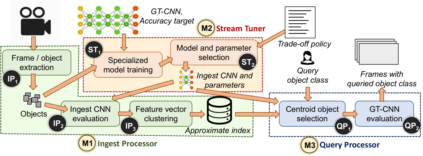
Because Focus targets large video datasets, a key requirement of Focus’ implementation is the ability to scale and distribute computation across many machines. To this end, we implement Focus as three loosely-coupled modules which handle each of its three key tasks. Figure 6 presents the architecture and the three key modules of Focus: the ingest processor (M1), the stream tuner (M2), and the query processor (M3). These modules can be flexibly deployed on different machines based on the video dataset size and the available hardware resources (such as GPUs). We describe each module in turn.
1 Ingest Processor
Focus’ ingest processor (M1) generates the approximate index (§1) for the input video stream. The work is distributed across many machines, with each machine running one worker process for each video stream’s ingestion. An ingest processor handles its input video stream with a four-stage pipeline: (i) extracting the moving objects from the video frames (IP1 in Figure 6), (ii) inferring the top-K indexes and the feature vectors of all detected objects with the ingest-time CNN (IP2 in Figure 6, §1), (iii) using the feature vector to cluster objects (IP3 in Figure 6, §3), and (iv) storing the top-K indexes of centroid objects in a database for efficient retrieval at query time.
An ingest processor is configured differently for static (fixed-angle) and moving cameras. For static cameras, we extract object boxes by subtracting each video frame from the background frame, which is obtained by averaging the frames in each hour of the video. We then index each object box with an ingest-time object classifier CNN. We accelerate the background subtraction with GPUs [14]. We use background subtraction for static cameras because running background subtraction with a cheap object classifier is much faster than running an ingest-time object detector CNN, and we find that both approaches have almost the same accuracy in detecting objects in static cameras. Hence, we choose the cheaper ingest option.
For moving cameras, we use a cheap, ingest-time object detector CNN (e.g., Tiny YOLO [127]) to generate the approximate indexes. We choose the object detection threshold (the threshold to determine if a box has an object) for the object detector CNN such that we do not miss objects in GT-CNN while minimizing spurious objects.
2 Stream Tuner
The stream tuner (M2) determines the ingest-time CNN and Focus’ parameters for each video stream (§4). It takes four inputs: the sampled frames/objects, the GT-CNN, the desired accuracy relative to the GT-CNN, and the tradeoff policy between ingest cost and query latency (§4). Whenever executed, the stream tuner: (i) generates the ground truth of the sampled frames/objects with the GT-CNN; (ii) trains specialized ingest-time CNNs based on the ground truth (ST1 in Figure 6); and (iii) selects the ingest-time CNN and Focus’ parameters (ST2 in Figure 6).
Focus executes the stream tuner for each video stream before launching the corresponding ingest processor. As the characteristics of video streams may change over time, Focus periodically launches the stream tuner to validate the accuracy of the selected parameters on sampled frames. The ingest-time CNN and the system parameters are re-tuned if necessary to meet the accuracy targets (e.g., [90]).
3 Query Processor
The task of the query processor is to return the video frames that contain the user’s queried object class. In response to a user query for class , the query processor first retrieves the centroid objects with matching approximate indexes (QP1 in Figure 6), and then uses the GT-CNN to determine the frames that do contain object class (QP2 in Figure 6, §1). The GT-CNN evaluation can be easily distributed across many machines, if needed.
We employ two optimizations to reduce the overhead of GT-CNN evaluation. First, we skip the GT-CNN evaluation for high-confidence indexes (§1). Second, we apply a query-specialized binary classifier [93] on the frames that need to be checked before invoking the GT-CNN. These two optimizations make the query processor more efficient by not running GT-CNN on all candidate centroid objects.
5 Evaluation
We evaluate our Focus prototype with more than 160 hours of videos from 14 real video streams that span traffic cameras, surveillance cameras, and news channels. Our main results are:
- 1.
- 2.
Focus provides a rich trade-off space between ingest cost and query latency. If a user wants to optimize for ingest cost, Focus is 65 cheaper on average (up to 96) than the Ingest-heavy baseline, while reducing query latency by 100 on average. If the goal is to optimize for query latency, Focus can achieve 202 (up to 698) faster queries than NoScope with 53 cheaper ingest. (§4).
1 Methodology
Software Tools. We use OpenCV 3.4.0 [13] to decode the videos into frames, and we feed the frames to our evaluated systems, Focus and NoScope. Focus runs and trains CNNs with Microsoft Cognitive Toolkit 2.4 [115], an open-source deep learning system. Our ingest processor (§1) stores the approximate index in MongoDB [11] for efficient retrieval at query time.
Video Datasets. We evaluate 14 video streams that span across traffic cameras, surveillance cameras, and news channels. We record each video stream for 12 hours to cover both day time and night time. Table 1 summarizes the video characteristics. We strengthen our evaluation by including down sampling (or frame skipping), one of the most straightforward approaches to reduce ingest cost and query latency, into our evaluation baseline. Specifically, as the vast majority of objects show up for at least one second in our evaluated videos, we evaluate each video at 1 fps instead of 30 fps. We find that the object detection results at these two frame rates are almost the same. Each video is split evenly into a training set and a test set. The training set is used to train video-specialized CNNs and select system parameters. We then evaluate the systems with the test set. In some figures, we show results for only eight representative videos to improve legibility.
| Type | Camera | Name | Description | |||
|---|---|---|---|---|---|---|
| auburn_c |
| |||||
| Traffic | Static | auburn_r |
| |||
| bellevue_d |
| |||||
| bellevue_r |
| |||||
| bend |
| |||||
| jackson_h |
| |||||
| jackson_ts |
| |||||
| Surveillance | Static |
|
| |||
|
| |||||
|
| |||||
| sittard |
| |||||
| News | Moving | cnn |
| |||
| foxnews |
| |||||
| msnbc |
|
Accuracy Target. We use YOLOv2 [127], a state-of-the-art object detector CNN, as our ground-truth CNN (GT-CNN): all objects detected by GT-CNN are considered to be the correct answers.44 4 We do not use the latest YOLOv3 or other object detector CNN such as FPN [107] as our GT-CNN because one of our baseline systems, NoScope, comes with the YOLOv2 code. Fundamentally, there is no restriction on the selection of GT-CNN for Focus. For each query, our default accuracy target is 99% recall and precision. To avoid overfitting, we use the training set of each video to explore system parameters with various recall/precision targets (i.e., 100%–95% with a 0.5% step), and we report the best system parameters that can actually achieve the recall/precision target on the test set. We also evaluate other recall/precision targets such as 97% and 95% (§5).
Baselines. We use baselines at two ends of the design spectrum: (1) Ingest-heavy, the baseline system that uses GT-CNN to analyze all frames at ingest time, and stores the results as an index for query; and (2) NoScope, a recent state-of-the-art querying system [93] that analyzes frames for the queried object class at query time. We also use a third baseline, Ingest-NoScope that uses NoScope’s techniques at ingest time. Specifically, Ingest-NoScope runs the binary classifiers of NoScope for all possible classes at ingest time, invokes GT-CNN if any of the binary classifiers cannot produce a high-confidence result, and stores the results as an index for query. To further strengthen the baselines, we augment all baseline systems with background subtraction, thus eliminating frames with no motion. As Focus is in the middle of the design spectrum, we compare Focus’ ingest cost with Ingest-heavy and Ingest-NoScope, and we compare Focus’ query latency with NoScope.
Metrics. We use two performance metrics. The first metric is ingest cost, the end-to-end machine time to ingest each video. The second metric is query latency, the end-to-end latency for an object class query. Specifically, for each video stream, we evaluate the object classes that collectively make up 95% of the detected objects in GT-CNN. We report the average query latency on these object classes. We do not evaluate the bottom 5% classes because they are often random erroneous results in GT-CNN (e.g., “broccoli” or “orange” in a traffic camera).
Both metrics include the time spent on all processing stages, such as detecting objects with background subtraction, running CNNs, clustering, reading and writing to the approximate index, etc. Similar to prior work [127, 93], we report the end-to-end execution time of each system while excluding the video decoding time, as the decoding time can be easily accelerated with GPUs or accelerators.
Experimental Platform. We run the experiments on Standard_NC6s_v2 instances on the Azure cloud. Each instance is equipped with a high-end GPU (NVIDIA Tesla P100), 6-core Intel Xeon CPU (E5-2690), 112 GB RAM, a 10 GbE NIC, and runs 64-bit Ubuntu 16.04 LTS.
2 End-to-End Performance
Static Cameras. We first show the end-to-end performance of Focus on static cameras when Focus aims to balance these two metrics (§4). Figure 7 compares the ingest cost of Focus and Ingest-NoScope with Ingest-heavy and the query latency of Focus with NoScope. We make three main observations.

First, Focus significantly improves query latency with a very small cost at ingest time. Focus achieves 162 speedup (on average) in query latency over NoScope with a very small ingest cost (57 cheaper than Ingest-heavy, on average), all the while retaining 99% recall and precision (not shown). Focus achieves two orders of magnitude speedup over NoScope because: (i) the ingest-time approximate indexing drastically narrows down the frames that need to be checked at query time; and (ii) the feature-based clustering further reduces the redundant work. In contrast, NoScope needs to go through all the frames at query time, which is especially inefficient for the object classes that appear infrequently. We conclude that Focus’ architecture provides a valuable trade-off between ingest cost and query latency.
Second, directly applying NoScope’s techniques at ingest time (Ingest-NoScope) does not save much cost over Ingest-heavy. There are two reasons for this: (1) While each binary classifier is relatively cheap, running multiple instances of binary classifiers (for all possible object classes) imposes non-trivial cost. (2) The system needs to invoke GT-CNN when any one of the binary classifiers cannot derive the correct answer. As a result, GT-CNN is invoked for most frames. Hence, the ingest cost of Focus is much cheaper than both, Ingest-heavy and Ingest-NoScope. This is because Focus’ architecture only needs to construct the approximate index at ingest time which can be done cheaply with an ingest-time CNN.
Third, Focus is effective across videos with varying characteristics. It makes queries 46 to 622 faster than NoScope with a very small ingest cost (35 to 92 cheaper than Ingest-heavy) among busy intersections (auburn_c, bellevue_d and jackson_h), normal intersections (auburn_r, bellevue_r, bend), a night street (jackson_ts), busy plazas (lausanne and sittard), a university street (oxford), and an aquarium (coral). The gains in query latency are smaller for some videos (auburn_r, bellevue_r, bend, and jackson_ts). This is because Focus’ ingest CNN is less accurate on these videos, and Focus selects more conservative parameters (e.g., a larger K such as 4–5 instead of 1–2) to attain the recall/precision targets. As a result, there is more work at query time for these videos. Nonetheless, Focus still achieves at least 40 speedup over NoScope in query latency. We conclude that the core techniques of Focus are general and effective on a variety of real-world videos.
Moving Cameras. We evaluate the applicability of Focus on moving cameras using three news channel video streams. These news videos were recorded with moving cameras and they change scenes between different news segments. For moving cameras, we use a cheap object detector (Tiny YOLO, which is 5 faster than YOLOv2 for the same input image size) as our ingest-time CNN. Figure 8 shows the end-to-end performance of Focus on moving cameras.

As the figure shows, Focus is effective in reducing query latency with only a modest ingest cost. Focus achieves a 49 speedup in query latency on average over NoScope, with ingest cost that is 5 cheaper than Ingest-heavy. We make two main observations. First, the ingest cost improvements on moving cameras (5) is lower than the ones on static cameras (57). This is because moving cameras require a detector CNN to detect objects, and it is more costly to run a cheap object detector (like Tiny YOLO) as opposed to using background subtraction to detect the objects and then classifying them using a cheap classifier CNN (like compressed ResNet18). Our design, however, does not preclude using much cheaper detectors than Tiny YOLO, and we can further reduce the ingest cost of moving cameras by exploring even cheaper object detector CNNs. Second, Focus’ techniques are very effective in reducing query latency on moving cameras. The approximate index generated by a cheap detector CNN significantly narrows down the frames that need to be checked at query time. We conclude that the techniques of Focus are general and can be applied to a wide range of object detection CNNs and camera types.
Averaging over both static and moving cameras, Focus’ ingest cost is 48 cheaper than Ingest-heavy and its queries are 125 faster than NoScope.
We now take a deeper look at Focus’ performance using representative static cameras.
3 Effect of Different Focus Components
Figure 9 shows the breakdown of query latency gains for two core techniques of Focus: (1) Approximate indexing, which indexes each object with the top-K results of the ingest-time CNN, and (2) Approximate indexing + Clustering, which adds feature-based clustering at ingest time to reduce redundant work at query time. We show the results that achieve at least 99% recall and precision. We make two observations.
First, approximate indexing is the major source of query latency improvement. This is because approximate indexing effectively eliminates irrelevant objects for each query and bypasses the query-time verification for high-confidence ingest predictions. As a result, only a small fraction of frames need to be resolved at query time. On average, approximate indexing alone is 114 faster than NoScope in query latency.
Second, clustering is a very effective technique to further reduce query latency. Using clustering (on top of approximate indexing) reduces the query latency by 195, significantly better than approximate indexing alone. We see that clustering is especially effective on surveillance videos (e.g., coral, lausanne, and oxford) because objects in these videos tend to stay longer in the camera (e.g., “person” on a plaza compared to “car” in traffic videos), and hence there is more redundancy in these videos. This gain comes with a negligible cost because we run our clustering algorithm (§3) on the otherwise idle CPUs of the ingest machine while the GPUs run the ingest-time CNN model.
4 Ingest Cost vs. Query Latency Trade-off
One of the important features of Focus is the flexibility to tune its system parameters to achieve different application goals (§4). Figure 10 (the zoom-in region of Figure 1) depicts three alternative settings for Focus that illustrate the trade-off space between ingest cost and query latency, using the oxford video stream: (1) Focus-Opt-Query, which optimizes for query latency by increasing ingest cost, (2) Focus-Balance, which is the default option that balances these two metrics (§4), and (3): Focus-Opt-Ingest, which is the opposite of Focus-Opt-Query. The results are shown relative to the Ingest-heavy and NoScope baselines. Each data label indicates its ingest cost is cheaper than Ingest-heavy, while its query latency is faster than NoScope.
As Figure 10 shows, Focus offers very good options in the trade-off space between ingest cost and query latency. Focus-Opt-Ingest is 90 cheaper than Ingest-heavy, and makes the query 403 faster than a query-optimized system (NoScope). On the other hand, Focus-Opt-Query reduces query latency even more (by 698) but it is still 53 cheaper than Ingest-heavy. As these points in the design space are all good options compared to the baselines, such flexibility enables a user to tailor Focus for different contexts. For example, a camera that requires fast turnaround time for queries can use Focus-Opt-Query, while a video stream that will be queried rarely would choose Focus-Opt-Ingest to reduce the amount of wasted ingest cost in exchange for longer query latencies.
Figure 11 shows the values for both Focus-Opt-Ingest (Opt-I) and Focus-Opt-Query (Opt-Q) for the representative videos. As the figure shows, the flexibility to make different trade-offs exists in most other videos. On average, Focus-Opt-Ingest is 65 (up to 96) cheaper than Ingest-heavy in ingest cost while providing 100 (up to 443) faster queries. Focus-Opt-Query makes queries 202 (up to 698) faster with a higher ingest cost (53 cheaper than Ingest-heavy). Note that there is no fundamental limitation on the spread between Focus-Opt-Query and Focus-Opt-Ingest as we can expand the search space for ingest-time CNNs to further optimize ingest cost at the expense of query latency (or vice versa). We conclude that Focus enables flexibly optimizing for ingest cost or query latency for application’s needs.
It is worth noting that the fraction of videos that get queried can affect the applicability of Focus, especially in the case where only a tiny fraction of videos gets queried. While Focus-Opt-Ingest can save the ingest cost by up to 96, it can be more costly than any purely query-time-only solution if the fraction of videos that gets queried is less than . In such a case, a user can still use Focus to significantly reduce query latency, but the cost of Focus can be higher than query-time-only solutions.
5 Sensitivity to Recall/Precision Target
Figure 12 illustrates Focus’ reduction in query latency compared to the baselines under different recall/precision targets. Other than the default 99% recall and precision target, we evaluate both Focus and NoScope with two lower targets, 97% and 95%.

We observe that with lower accuracy targets, the query latency improvement decreases slightly for most videos, while the ingest cost improvement does not change much (not graphed). The ingest cost is not sensitive to the accuracy target because Focus still runs similar ingest CNNs. NoScope can however apply more aggressive query-time optimization to reduce query latency given lower accuracy targets. This decreases Focus’ improvement over NoScope for several videos. On average, Focus is faster than NoScope in query latency by 195, 167, and 169 with recall/precision of 99%, 97%, and 95%, respectively. We conclude that Focus’ techniques can achieve significant improvements on query latency, irrespective of recall/precision targets.
6 Sensitivity to Object Class Numbers
We use the 1000 object classes in the ImageNet dataset [133] to study the sensitivity of Focus’ performance to the number of object classes (compared to the 80 default object classes in the COCO [108] dataset). Our result shows that Focus is 15 faster (on average) in query latency and 57 cheaper (on average) in ingest cost than the baseline systems, while achieving 99% recall and precision. We observe that the query latency improvements with 1000 object classes is lower than the ones with 80 object classes. The reason is that ingest-time CNNs are less accurate on more object classes, and we need to select a larger K to achieve the target recall. Nonetheless, the improvements of Focus are robust with more object classes as Focus is over one order of magnitude faster than the baseline systems when differentiating 1000 object classes.
6 Other Applications
Applications that leverage CNNs to process large and continuously growing data share similar challenges as Focus. Examples of such applications are:
1) Video and audio. Other than querying for objects, many emerging video applications are also based on CNNs, such as event detection (e.g., [169]), emotion recognition (e.g., [91]), video classification (e.g., [94]), and face recognition (e.g., [137]). Audio applications such as speech recognition (e.g., [21]) are also based on CNNs.
2) Bioinformatics and geoinformatics. Many bioinformatics and geoinformatics systems leverage CNNs to process a large dataset, such as anomaly classification in biomedical imaging (e.g., [106, 131]), information decoding in biomedical signal recordings (e.g., [145]), and pattern recognition in satellite imagery (e.g., [24, 45]).
Naturally, these applications need to answer user-specified queries, such as “find all brain signal recordings with a particular perception” or “find all audio recordings with a particular keyword”. Supporting these queries faces similar challenges to Focus, as a system either: (i) generates a precise index at ingest time, which incurs high cost; or (ii) does most of the heavy-lifting at query time, which results in high query latency. Hence, Focus’ architecture offers a low-cost and low-latency option: building an approximate index with cheap CNNs at ingest time and generating precise results based on the approximate index at query time. While the indexing structure may need to be adapted to different applications, we believe Focus’ architecture and techniques can benefit many of these emerging applications.
7 Summary
Answering queries of the form, find me frames that contain objects of class X, is an important workload on recorded video datasets. Such queries are used by analysts and investigators for various immediate purposes, and it is crucial to answer them with low latency and low cost. This chapter presents Focus, a system that flexibly divides the query processing work between ingest time and query time. Focus performs low-cost ingest-time analytics on live video that later facilitates low-latency queries on the recorded videos. At ingest time, Focus uses cheap CNNs to construct an approximate index of all possible object classes in each frame to retain high recall. At query time, Focus leverages this approximate index to provide low latency, but compensates for the lower precision by judiciously using expensive CNNs. This architecture enables orders-of-magnitude faster queries with only a small investment at ingest time, and allows flexibly trading off ingest cost and query latency. Our evaluations using real-world videos from traffic, surveillance, and news domains show that Focus reduces ingest cost on average by (up to ) and makes queries on average (up to ) faster compared to state-of-the-art baselines. We conclude that Focus’ architecture and techniques make it a highly practical and effective approach to querying large video datasets. We hope that the ideas and insights behind Focus can be applied to designing efficient systems for many other forms of querying on large and continuously-growing datasets in many domains, such as audio, bioinformatics, and geoinformatics.
Chapter 4 ML Training over Geo-Distributed Data
As Chapter § Machine Learning Systems
for Highly-Distributed and Rapidly-Growing Data discusses, many ML applications
analyze massive amounts of data from user activities, pictures,
videos, etc., which are generated at very rapid rates, all
over the world. Many large organizations, such as
Google [64], Microsoft [114], and
Amazon [25], operate tens of data centers globally to
minimize their service latency to end-users, and store massive
quantities of data all over the
globe [161, 124, 122, 165, 159, 68, 74, 84, 97, 160].
A commonly-used approach to run an ML application over such rapidly generated data is to centralize all data into one data center over wide-area networks (WANs) before running the ML application [40, 152, 103, 29]. However, this approach can be prohibitively difficult because: (1) WAN bandwidth is a scarce resource, and hence moving all data can be extremely slow [122, 40]. Furthermore, the fast growing rate of image and video generation will eventually saturate the total WAN bandwidth, whose growth has been decelerating for many years [151, 161]. (2) Privacy and data sovereignty laws in some countries prohibit transmission of raw data across national or continental borders [161, 160, 40].
This motivates the need to distribute an ML system across multiple data centers, globally. In such a system, large amounts of raw data are stored locally in different data centers, and the ML algorithms running over the distributed data communicate between data centers using WANs. Unfortunately, existing large-scale distributed ML systems [46, 167, 113, 110, 20, 104] are suitable only for data residing within a single data center. Our experiments using three state-of-the-art distributed ML systems (Bösen [162], IterStore [51], and GeePS [52]) show that operating these systems across as few as two data centers (over WANs) can cause a slowdown of 1.8–53.7 (see Section 2 and Section 5) relative to their performance within a data center (over LANs). Existing systems that do address challenges in geo-distributed data analytics [161, 124, 122, 159, 74, 84, 97, 40, 160] do not consider the broad class of important, sophisticated ML algorithms commonly run on ML systems — they focus instead on other types of computation, e.g., map-reduce or SQL.
Our goal in this chapter is to develop a geo-distributed ML system that (1) minimizes communication over WANs, so that the system is not bottlenecked by the scarce WAN bandwidth; and (2) is general enough to be applicable to a wide variety of ML algorithms, without requiring any changes to the algorithms themselves.
To achieve these goals, such a system needs to address two key challenges. First, to efficiently utilize the limited (and heterogeneous) WAN bandwidth, we need to find an effective communication model that minimizes communication over WANs but still retains the correctness guarantee for an ML algorithm. This is difficult because ML algorithms typically require extensive communication to exchange updates that keep the global ML model sufficiently consistent across data centers. These updates are required to be timely, irrespective of the available network bandwidth, to ensure algorithm correctness. Second, we need to design a general system that effectively handles WAN communication for ML algorithms without requiring any algorithm changes. This is challenging because the communication patterns vary significantly across different ML algorithms [148, 153, 129, 88, 118, 144]. Altering the communication across systems can lead to different tradeoffs and consequences for different algorithms [175].
In this chapter, we introduce Gaia, a new general, geo-distributed ML system that is designed to efficiently operate over a collection of data centers. Gaia builds on the widely used parameter server architecture (e.g., [75, 51, 167, 50, 104, 162, 46, 20, 23, 54]) that provides ML worker machines with a distributed global shared memory abstraction for the ML model parameters they collectively train until convergence to fit the input data. The key idea of Gaia is to maintain an approximately-correct copy of the global ML model within each data center, and dynamically eliminate any unnecessary communication between data centers. Gaia enables this by decoupling the synchronization (i.e., communication/consistency) model within a data center from the synchronization model between different data centers. This differentiation allows Gaia to run a conventional synchronization model [53, 162, 75] that maximizes utilization of the more-freely-available LAN bandwidth within a data center. At the same time, across different data centers, Gaia employs a new synchronization model, called Approximate Synchronous Parallel (ASP), which makes more efficient use of the scarce and heterogeneous WAN bandwidth. By ensuring that each ML model copy in different data centers is approximately correct based on a precise notion defined by ASP, we guarantee ML algorithm convergence.
ASP is based on a key finding that the vast majority of updates to the global ML model parameters from each ML worker machine are insignificant. For example, our study of three classes of ML algorithms shows that more than 95% of the updates produce less than a 1% change to the parameter value. With ASP, these insignificant updates to the same parameter within a data center are aggregated (and thus not communicated to other data centers) until the aggregated updates are significant enough. ASP allows the ML programmer to specify the function and the threshold to determine the significance of updates for each ML algorithm, while providing default configurations for unmodified ML programs. For example, the programmer can specify that all updates that produce more than a 1% change are significant. ASP ensures all significant updates are synchronized across all model copies in a timely manner. It dynamically adapts communication to the available WAN bandwidth between pairs of data centers and uses special selective barrier and mirror clock control messages to ensure algorithm convergence even during a period of sudden fall (negative spike) in available WAN bandwidth.
In contrast to a state-of-the-art communication-efficient synchronization model, Stale Synchronous Parallel (SSP) [75], which bounds how stale (i.e., old) a parameter can be, ASP bounds how inaccurate a parameter can be, in comparison to the most up-to-date value. Hence, it provides high flexibility in performing (or not performing) updates, as the server can delay synchronization indefinitely as long as the aggregated update is insignificant.
We build two prototypes of Gaia on top of two state-of-the-art parameter server systems, one specialized for CPUs [51] and another specialized for GPUs [52]. We deploy Gaia across 11 regions on Amazon EC2, and on a local cluster that emulates the WAN bandwidth across different Amazon EC2 regions. Our evaluation with three popular classes of ML algorithms shows that, compared to two state-of-the-art parameter server systems [51, 52] deployed on WANs, Gaia: (1) significantly improves performance, by 1.8–53.5, (2) has performance within 0.94–1.40 of running the same ML algorithm on a LAN in a single data center, and (3) significantly reduces the monetary cost of running the same ML algorithm on WANs, by 2.6–59.0.
1 Motivation
To further motivate our work, we discuss WAN bandwidth constraints and study the performance implications of running two state-of-the-art ML systems over WANs.
1 WAN Network Bandwidth and Cost
WAN bandwidth is a very scarce resource [100, 124, 161] relative to LAN bandwidth. Moreover, the high cost of adding network bandwidth has resulted in a deceleration of WAN bandwidth growth. The Internet capacity growth has fallen steadily for many years, and the annual growth rates have lately settled into the low-30 percent range [151].
To quantify the scarcity of WAN bandwidth between data centers, we measure the network bandwidth between all pairs of Amazon EC2 sites in 11 different regions (Virginia, California, Oregon, Ireland, Frankfurt, Tokyo, Seoul, Singapore, Sydney, Mumbai, and São Paulo). We use iperf3 [58] to measure the network bandwidth of each pair of different regions for five rounds, and then calculate the average bandwidth. Figure 1 shows the average network bandwidth between each pair of different regions. We make two observations.

First, the WAN bandwidth between data centers is 15 smaller than the LAN bandwidth within a data center on average, and up to 60 smaller in the worst case (for Singapore ↔ São Paulo). Second, the WAN bandwidth varies significantly between different regions. The WAN bandwidth between geographically-close regions (e.g., Oregon ↔ California or Tokyo ↔ Seoul) is up to 12 of the bandwidth between distant regions (e.g., Singapore ↔ São Paulo). As Section 2 shows, the scarcity and variation of the WAN bandwidth can significantly degrade the performance of state-of-the-art ML systems.
Another important challenge imposed by WANs is the monetary cost of communication. In data centers, the cost of WANs far exceeds the cost of a LAN and makes up a significant fraction of the overall cost [66]. Cloud service providers, such as Amazon EC2, charge an extra fee for WAN communication while providing LAN communication free of charge. The cost of WAN communication can be much higher than the cost of the machines themselves. For example, the cost of two machines in Amazon EC2 communicating at the rate of the average WAN bandwidth between data centers is up to 38 of the cost of renting these two machines [26]. These costs make running ML algorithms on WANs much more expensive than running them on a LAN.
2 ML System Performance on WANs
We study the performance implications of deploying distributed ML systems on WANs using two state-of-the-art parameter server systems, IterStore [51] and Bösen [162]. Our experiments are conducted on our local 22-node cluster that emulates the WAN bandwidth between Amazon EC2 data centers, the accuracy of which is validated against a real Amazon EC2 deployment (see Section 2 for details). We run the same ML application, Matrix Factorization [60] (Section 2), on both systems.
For each system, we evaluate both BSP and SSP as the synchronization model (Section 1), with four deployment settings: (1) LAN, deployment within a single data center, (2) EC2-ALL, deployment across 11 aforementioned EC2 regions, (3) V/C WAN, deployment across two data centers that have the same WAN bandwidth as that between Virginia and California (Figure 1), representing a distributed ML setting within a continent, and (4) S/S WAN, deployment across two data centers that have the same WAN bandwidth as that between Singapore and São Paulo, representing the lowest WAN bandwidth between any two Amazon EC2 regions.
Figure 2 shows the normalized execution time until algorithm convergence across the four deployment settings. All results are normalized to IterStore using BSP on a LAN. The data label on each bar represents how much slower the WAN setting is than its respective LAN setting for the given system, e.g., Bösen-BSP on EC2-ALL is 5.9 slower than Bösen-BSP on LAN.

As we see, both systems suffer significant performance degradation when deployed across multiple data centers. When using BSP, IterStore is 3.5 to 23.8 slower on WANs than it is on a LAN, and Bösen is 4.4 to 24.2 slower. While using SSP can reduce overall execution times of both systems, both systems still show significant slowdown when run on WANs (2.3 to 13.7 for IterStore, and 4.3 to 26.8 for Bösen). We conclude that simply running state-of-the-art distributed ML systems on WANs can seriously slow down ML applications, and thus we need a new distributed ML system that can be effectively deployed on WANs.
2 Our Approach: Gaia
We introduce Gaia, a general ML system that can be effectively deployed on WANs to address the increasing need to run ML applications directly on geo-distributed data. We identify two key challenges in designing such a system (Section 1). We then introduce the system architecture of Gaia, which differentiates the communication within a data center from the communication between different centers (Section 2). Our approach is based on the key empirical finding that the vast majority of communication within an ML system results in insignificant changes to the state of the global model (Section 3). In light of this finding, we design a new ML synchronization model, called Approximate Synchronous Parallel (ASP), which can eliminate the insignificant communication while ensuring the convergence and accuracy of ML algorithms. We describe ASP in detail in Section 4. Finally, Section 5 summarizes our theoretical analysis of how ASP guarantees algorithm convergence for a widely-used ML algorithm, stochastic gradient descent (SGD) (the full proof is in Appendix 4.A).
1 Key Challenges
There are two key challenges in designing a general and effective ML system on WANs.
Challenge 1. How to effectively communicate over WANs while retaining algorithm convergence and accuracy? As we see above, state-of-the-art distributed ML systems can overwhelm the scarce WAN bandwidth, causing significant slowdowns. We need a mechanism that significantly reduces the communication between data centers so that the system can provide competitive performance. However, reducing communication can affect the accuracy of an ML algorithm. A poor choice of synchronization model in a distributed ML system can prevent the ML algorithm from converging to the optimal point (i.e., the best model to explain or fit the input data) that one can achieve when using a proper synchronization model [38, 126]. Thus, we need a mechanism that can reduce communication intensity while ensuring that the communication occurs in a timely manner, even when the network bandwidth is extremely stringent. This mechanism should provably guarantee algorithm convergence irrespective of the network conditions.
Challenge 2. How to make the system generic and work for ML algorithms without requiring modification? Developing an effective ML algorithm takes significant effort and experience, making it a large burden for the ML algorithm developers to change the algorithm when deploying it on WANs. Our system should work across a wide variety of ML algorithms, preferably without any change to the algorithms themselves. This is challenging because different ML algorithms have different communication patterns, and the implication of reducing communication can vary significantly among them [148, 153, 129, 88, 118, 144, 175].
2 Gaia System Overview
We propose a new ML system, Gaia, that addresses the two key challenges in designing a general and effective ML system on WANs. Gaia is built on top the popular parameter server architecture, which is proven to be effective on a wide variety of ML algorithms (e.g., [75, 51, 167, 50, 104, 162, 46, 20, 23, 54]). As discussed in Section 1, in the parameter server architecture, all worker machines synchronize with each other through parameter servers to ensure that the global model state is up-to-date. While this architecture guarantees algorithm convergence, it also requires substantial communication between worker machines and parameter servers. To make Gaia effective on WANs while fully utilizing the abundant LAN bandwidth, we design a new system architecture to decouple the synchronization within a data center (LANs) from the synchronization across different data centers (WANs).
Figure 3 shows an overview of Gaia. In Gaia, each data center has some worker machines and parameter servers. Each worker machine processes a shard of the input data stored in its data center to achieve data parallelism (Section 1). The parameter servers in each data center collectively maintain a version of the global model copy (❶), and each parameter server handles a shard of this global model copy. A worker machine only READs and UPDATEs the global model copy in its data center.
To reduce the communication overhead over WANs, the global model copy in each data center is only approximately correct. This design enables us to eliminate the insignificant, and thus unnecessary, communication across different data centers. We design a new synchronization model, called Approximate Synchronous Parallel (ASP ❷), between parameter servers across different data centers to ensure that each global model copy is approximately correct even with very low WAN bandwidth. Section 4 describes the details of ASP. On the other hand, worker machines and parameter servers within a data center synchronize with each other using the conventional BSP (Bulk Synchronous Parallel) or SSP (Stale Synchronous Parallel) models (❸). These models allow worker machines to quickly observe fresh updates that happen within a data center. Furthermore, worker machines and parameter servers within a data center can employ more aggressive communication schemes such as sending updates early and often [53, 162] to fully utilize the abundant (and free) network bandwidth on a LAN.
3 Study of Update Significance
As discussed above, Gaia reduces the communication overhead over WANs by eliminating insignificant communication. To understand the benefit of our approach, we study the significance of the updates sent from worker machines to parameter servers. We study three classes of popular ML algorithms: Matrix Factorization (MF) [60], Topic Modeling (TM) [34], and Image Classification (IC) [101] (see Section 2 for descriptions). We run all the algorithms until convergence, analyze all the updates sent from worker machines to parameter servers, and compare the change they cause on the parameter value when the servers receive them. We define an update to be significant if it causes % change on the parameter value, and we vary , the significance threshold, between 0.01 and 10. Figure 4 shows the percentage of insignificant updates among all updates, for different values of .

As we see, the vast majority of updates in these algorithms are insignificant. Assuming the significance threshold is 1%, 95.2% / 95.6% / 97.0% of all updates are insignificant for MF / TM / IC. When we relax the significance threshold to 5%, 98.8% / 96.1% / 99.3% of all updates are insignificant. Thus, most of the communication changes the ML model state only very slightly.
It is worth noting that our finding is consistent with the findings of prior work [55, 57, 110, 171, 96] on other ML algorithms, such as PageRank and Lasso. These works observe that in these ML algorithms, not all model parameters converge to their optimal value within the same number iterations — a property called non-uniform convergence [168]. Instead of examining the convergence rate, we quantify the significance of updates with various significance thresholds, which provides a unique opportunity to reduce the communication over WANs.
4 Approximate Synchronous Parallel
The goal of our new synchronization model, Approximate Synchronous Parallel (ASP), is to ensure that the global model copy in each data center is approximately correct. In this model, a parameter server shares only the significant updates with other data centers, and ASP ensures that these updates can be seen by all data centers in a timely fashion. ASP achieves this goal by using three techniques: (1) the significance filter, (2) ASP selective barrier, and (3) ASP mirror clock. We describe them in order.
The significance filter. ASP takes two inputs from an ML programmer to determine whether or not an update is significant. They are: (1) a significance function and (2) an initial significance threshold. The significance function returns the significance of each update. We define an update as significant if its significance is larger than the threshold. For example, an ML programmer can define the significance function as the update’s magnitude relative to the current value (), and set the initial significance threshold to 1%. The significance function can be more sophisticated if the impact of parameter changes to the model is not linear, or the importance of parameters is non-uniform (see Section 3). A parameter server aggregates updates from the local worker machines and shares the aggregated updates with other data centers when the aggregated updates become significant. To ensure that the algorithm can converge to the optimal point, ASP automatically reduces the significance threshold over time (specifically, if the original threshold is , then the threshold at iteration of the ML algorithm is ).
ASP selective barrier. While we can greatly reduce the communication overhead over WANs by sending only the significant updates, the WAN bandwidth might still be insufficient for such updates. In such a case, the significant updates can arrive too late, and we might not be able to bound the deviation between different global model copies. ASP handles this case with the ASP selective barrier (Figure 5(a)) control message. When a parameter server receives the significant updates (❶) at a rate that is higher than the WAN bandwidth can support, the parameter server first sends the indexes of these significant updates (as opposed to sending both the indexes and the update values together) via an ASP selective barrier (❷) to the other data centers. The receiver of an ASP selective barrier blocks its local worker from reading the specified parameters until it receives the significant updates from the sender of the barrier. This technique ensures that all worker machines in each data center are aware of the significant updates after a bounded network latency, and they wait only for these updates. The worker machines can make progress as long as they do not depend on any of these parameters.


Mirror clock. The ASP select barrier ensures that the latency of the significant updates is no more than the network latency. However, it assumes that 1) the underlying WAN bandwidth and latency are fixed so that the network latency can be bounded, and 2) such latency is short enough so that other data centers can be aware of them in time. In practice, WAN bandwidth can fluctuate over time [77], and the WAN latency can be intolerably high for some ML algorithms. Worse still, the ASP selective barrier messages could experience long delay when the network packets are dropped on WAN. We need a mechanism to guarantee that the worker machines are aware of the significant updates in time, irrespective of the WAN bandwidth or latency.
We use the mirror clock (Figure 5(b)) to provide this guarantee. When each parameter server receives all the updates from its local worker machines at the end of a clock (e.g., an iteration), it reports its clock to the servers that are in charge of the same parameters in the other data centers. When a server detects its clock is ahead of the slowest server that shares the same parameters by a predefined threshold (data center staleness), the server blocks its local worker machines from reading its parameters until the slowest mirror server catches up. In the example of Figure 5(b), the server clock in Data Center 1 is , while the server clock in Data Center 2 is . As their difference reaches the predefined limit, the server in Data Center 2 blocks its local worker from reading its parameters. This mechanism is similar to the concept of SSP [75], but we use it only as the last resort to guarantee algorithm convergence.
5 Summary of Convergence Proof
In this section, we summarize our proof showing that a popular, broad class of ML algorithms are guaranteed to converge under our new ASP synchronization model. The class we consider are ML algorithms expressed as convex optimization problems that are solved using distributed stochastic gradient descent.
The proof follows the outline of prior work on SSP [75], with a new challenge, i.e., our new ASP synchronization model allows the synchronization of insignificant updates to be delayed indefinitely. To prove algorithm convergence, our goal is to show that the distributed execution of an ML algorithm results in a set of parameter values that are very close (practically identical) to the values that would be obtained under a serialized execution.
Let denote the objective function of an optimization problem, whose goal is to minimize . Let denote the sequence of noisy (i.e., inaccurate) views of the parameters, where is the index of each view over time. Let denote the value that minimizes . Intuitively, we would like to approach as . We call the difference between and regret. We can prove approaches as by proving that the average regret, as .
Mathematically, the above intuition is formulated with Theorem 1. The details of the proof and the notations are in Appendix 4.A.
Theorem 1.
(Convergence of SGD under ASP). Suppose that, in order to compute the minimizer of a convex function , with , convex, we use stochastic gradient descent on one component at a time. Suppose also that 1) the algorithm is distributed in data centers, each of which uses machines, 2) within each data center, the SSP protocol is used, with a fixed staleness of , and 3) a fixed mirror clock difference is allowed between any two data centers. Let , where the step size decreases as and the significance threshold decreases as . If we further assume that: and . Then, as , the regret and therefore .
3 Implementation
We introduce the key components of Gaia in Section 1, and discuss the operation and design of individual components in the remaining sections.
1 Gaia System Key Components
Figure 6 presents the key components of Gaia. All of the key components are implemented in the parameter servers, and can be transparent to the ML programs and the worker machines. As we discuss above, we decouple the synchronization within a data center (LANs) from the synchronization across different data centers (WANs). The local server (❶) in each parameter server handles the synchronization between the worker machines in the same data center using the conventional BSP or SSP models. On the other hand, the mirror server (❷) and the mirror client (❸) handle the synchronization with other data centers using our ASP model. Each of these three components runs as an individual thread.
2 System Operations and Communication
We present a walkthrough of major system operations and communication.
UPDATE from a worker machine. When a local server (❶) receives a parameter update from a worker machine, it updates the parameter in its parameter store (❹), which maintains the parameter value and its accumulated update. The local server then invokes the significance filter (❺) to determine whether or not the accumulated update of this parameter is significant. If it is, the significance filter sends a MIRROR UPDATE request to the mirror client (❸) and resets the accumulated update for this parameter.
Messages from the significance filter. The significance filter sends out three types of messages. First, as discussed above, it sends a MIRROR UPDATE request to the mirror client through the data queue (❼). Second, when the significance filter detects that the arrival rate of significant updates is higher than the underlying WAN bandwidth that it monitors at every iteration, it first sends an ASP Barrier (Section 4) to the control queue (❻) before sending the MIRROR UPDATE. The mirror client (❸) prioritizes the control queue over the data queue, so that the barrier is sent out earlier than the update. Third, to maintain the mirror clock (Section 4), the significance filter also sends a MIRROR CLOCK request to the control queue at the end of each clock in the local server.
Operations in the mirror client. The mirror client thread wakes up when there is a request from the control queue or the data queue. Upon waking up, the mirror client walks through the queues, packs together the messages to the same destination, and sends them.
Operations in the mirror server. The mirror server handles above messages (MIRROR UPDATE, ASP BARRIER, and MIRROR CLOCK) according to our ASP model. For MIRROR UPDATE, it applies the update to the corresponding parameter in the parameter store. For ASP BARRIER, it sets a flag in the parameter store to block the corresponding parameter from being read until it receives the corresponding MIRROR UPDATE. For MIRROR CLOCK, the mirror server updates its local mirror clock state for each parameter server in other data centers, and enforces the predefined clock difference threshold (Section 4).
3 Advanced Significance Functions
As we discuss in Section 4, the significance filter allows the ML programmer to specify a custom significance function to calculate the significance of each update. By providing an advanced significance function, Gaia can be more effective at eliminating the insignificant communication. If several parameters are always referenced together to calculate the next update, the significance function can take into account the values of all these parameters. For example, if three parameters , , and are always used as in an ML algorithm, the significance of , , and can be calculated as the change on . If one of them is 0, any change in another parameter, however large it may be, is insignificant. Similar principles can be applied to model parameters that are non-linear or non-uniform. For unmodified ML programs, the system applies default significance functions, such as the relative magnitude of an update for each parameter.
4 Tuning of Significance Thresholds
The user of Gaia can specify two different goals for Gaia: (1) speed up algorithm convergence by fully utilizing the available WAN bandwidth and (2) minimize the communication cost on WANs. In order to achieve either of these goals, the significance filter maintains two significance thresholds and dynamically tunes these thresholds. The first threshold is the hard significance threshold. The purpose of this threshold is to guarantee ML algorithm convergence. As we discuss in our theoretical analysis (Section 5), the initial threshold is provided by the ML programmer or a default system setting, and the significance filter reduces it over time. Specifically, the significance threshold decreases whenever the learning rate decreases. Every update whose significance is above the hard threshold is guaranteed to be sent to other data centers. The second threshold is the soft significance threshold. The purpose of it is to use underutilized WAN bandwidth to speed up convergence. This threshold is tuned based on the arrival rate of the significant updates and the underlying WAN bandwidth. When the user chooses to optimize the first goal (speed up algorithm convergence), the system lowers the soft significance threshold whenever there is underutilized WAN bandwidth. The updates whose significance is larger than the soft significance threshold are sent in a best-effort manner. On the other hand, if the goal of the system is to minimize the WAN communication costs, the soft significance threshold is not activated.
While the configuration of the initial hard threshold depends on how error tolerant each ML algorithm is, a simple and conservative threshold (such as 1%–2%) is likely to work in most cases. This is because most ML algorithms initialize their parameters with random values, and make large changes to their model parameters at early phases. Thus, they are more error tolerant at the beginning. As Gaia reduces the threshold over time, its accuracy loss is limited. Typically, the ML programmer selects the initial hard threshold by running Gaia locally with several values, and then selects the threshold value that can achieve target model accuracy (e.g., the accuracy of BSP) while minimizing network communication. An ML expert can choose a more aggressive threshold based on domain knowledge of the ML algorithm.
5 Overlay Network and Hub
While Gaia can eliminate the insignificant updates, each data center needs to broadcast the significant updates to all the other data centers. This broadcast-based communication could limit the scalability of Gaia when we deploy Gaia to many data centers. To make Gaia more scalable with more data centers, we use the concept of overlay networks [111].
As we discuss in Section 1, the WAN bandwidth between geographically-close regions is much higher than that between distant regions. In light of this, Gaia supports having geographically-close data centers form a data center group. Servers in a data center group send their significant updates only to the other servers in the same group. Each group has hub data centers that are in charge of aggregating all the significant updates within the group, and sending to the hubs of the other groups. Similarly, a hub data center broadcasts the aggregated significant updates from other groups to the other data centers within its group. Each data center group can designate different hubs for communication with different data center groups, so the system can utilize more links within a data center group. For example, the data centers in Virginia, California, and Oregon can form a data center group and assign the data center in Virginia as the hub to communicate with the data centers in Europe and the data center in Oregon as the hub to communicate with the data centers is Asia. This design allows Gaia to broadcast the significant updates with lower communication cost.
4 Methodology
1 Experiment Platforms
We use three different platforms for our evaluation.
Amazon-EC2. We deploy Gaia to 22 machines spread across 11 EC2 regions as we show in Figure 1. In each EC2 region we start two instances of type c4.4xlarge or m4.4xlarge [26], depending on their availability. Both types of instances have 16 CPU cores and at least 30GB RAM, running 64-bit Ubuntu 14.04 LTS (HVM). In all, our deployment uses 352 CPU cores and 1204 GB RAM.
Emulation-EC2. As the monetary cost of running all experiments on EC2 is too high, we run some experiments on our local cluster that emulates the computation power and WAN bandwidth of EC2. We use the same number of machines (22) in our local cluster. Each machine is equipped with a 16-core Intel Xeon CPU (E5-2698), an NVIDIA Titan X GPU, 64GB RAM, a 40GbE NIC, and runs the same OS as above. The computation power and the LAN speeds of our machines are higher than the ones we get from EC2, so we slow down the CPU and LAN speeds to match the speeds on EC2. We model the measured EC2 WAN bandwidth (Figure 1) with the Linux Traffic Control tool [10]. As Section 1 shows, our emulation platform gives very similar results to the results from our real EC2 deployment.
Emulation-Full-Speed. We run some of our experiments on our local cluster that emulates the WAN bandwidth of EC2 at full speed. We use the same settings as Emulation-EC2 except we do not slow down the CPUs and the LAN. We use this platform to show the results of deployments with more powerful nodes.
2 Applications
We evaluate Gaia with three popular ML applications.
Matrix Factorization (MF) is a technique commonly used in recommender systems, e.g., systems that recommend movies to users on Netflix (a.k.a. collaborative filtering) [60]. Its goal is to discover latent interactions between two entities, such as users and movies, via matrix factorization. For example, input data can be a partially filled matrix , where every entry is a user’s rating for a movie, each row corresponding to a user, and each column corresponding to a specific movie. Matrix factorization factorizes into factor matrices and such that their product approximates (i.e., ). Like other systems [71, 175, 51], we implement MF using the stochastic gradient descent (SGD) algorithm. Each worker is assigned a portion of the known entries in . The matrix is stored locally in each worker, and the matrix is stored in parameter servers. Our experiments use the Netflix dataset, a 480K-by-18K sparse matrix with 100M known entries. They are configured to factor the matrix into the product of two matrices, each with rank 500.
Topic Modeling (TM) is an unsupervised method for discovering hidden semantic structures (topics) in an unstructured collection of documents, each consisting of a bag (multi-set) of words [34]. TM discovers the topics via word co-occurrence. For example, “policy” is more likely to co-occur with “government” than “bacteria”, and thus “policy” and “government” are categorized to the same topic associated with political terms. Further, a document with many instances of “policy” would be assigned a topic distribution that peaks for the politics-related topics. TM learns the hidden topics and the documents’ associations with those topics jointly. Common applications for TM include community detection in social networks and news categorizations. We implement our TM solver using collapsed Gibbs sampling [67]. We use the Nytimes dataset [117], which has 100M words in 300K documents with a vocabulary size of 100K. Our experiments classify words and documents into 500 topics.
Image Classification (IC) is a task to classify images into categories, and the state-of-the-art approach is using deep learning and convolutional neural networks (CNNs) [101]. Given a set of images with known categories (training data), the ML algorithm trains a CNN to learn the relationship between the image features and their categories. The trained CNN is then used to predict the categories of another set of images (test data). We use GoogLeNet [146], one of the state-of-the-art CNNs as our model. We train GoogLeNet using stochastic gradient descent with back propagation [132]. As training a CNN with a large number of images requires substantial computation, doing so on CPUs can take hundreds of machines over a week [46]. Instead, we use distributed GPUs with a popular deep learning framework, Caffe [89], which is hosted by a state-of-the-art GPU-specialized parameter server system, GeePS [52]. Our experiments use the ImageNet Large Scale Visual Recognition Challenge 2012 (ILSVRC12) [133] dataset, which consists of 1.3M training images and 50K test images. Each image is labeled as one of the 1,000 pre-defined categories.
3 Performance Metrics and Algorithm Convergence Criteria
We use two performance metrics to evaluate the effectiveness of a globally distributed ML system. The first metric is the execution time until algorithm convergence. We use the following algorithm convergence criterion, based on guidance from our ML experts: if the value of the objective function (the objective value) in an algorithm changes by less than 2% over the course of 10 iterations, we declare that the algorithm has converged [71]. In order to ensure that each algorithm accurately converges to the optimal point, we first run each algorithm on our local cluster until it converges, and we record the absolute objective value. The execution time of each setting is the time it takes to converge to this absolute objective value.
The second metric is the cost of algorithm convergence. We calculate the cost based on the cost model of Amazon EC2 [26], including the cost of the server time and the cost of data transfer on WANs. We use the on-demand pricing of Amazon EC2 published for January 2017 as our cost model [26]. As the pricing might change over time, we provide the details of the cost model in Table 1. The CPU instance is c4.4xlarge or m4.4xlarge, depending on the availability in each EC2 region. The GPU instance is g2.8xlarge. The low-cost instance (m4.xlarge) is the one used for centralizing input data. All the instance costs are shown in USD per hour. All WAN data transfer costs are shown in USD per GB.
| Region |
|
|
|
|
| ||||||||||
|---|---|---|---|---|---|---|---|---|---|---|---|---|---|---|---|
| Virginia | $0.86 | $2.60 | $0.22 | $0.02 | $0.01 | ||||||||||
| California | $1.01 | $2.81 | $0.22 | $0.02 | $0.01 | ||||||||||
| Oregon | $0.86 | $2.60 | $0.22 | $0.02 | $0.01 | ||||||||||
| Ireland | $0.95 | $2.81 | $0.24 | $0.02 | $0.01 | ||||||||||
| Frankfurt | $1.03 | $3.09 | $0.26 | $0.02 | $0.01 | ||||||||||
| Tokyo | $1.11 | $3.59 | $0.27 | $0.09 | $0.01 | ||||||||||
| Seoul | $1.06 | $3.59 | $0.28 | $0.08 | $0.01 | ||||||||||
| Singapore | $1.07 | $4.00 | $0.27 | $0.09 | $0.01 | ||||||||||
| Sydney | $1.08 | $3.59 | $0.27 | $0.14 | $0.01 | ||||||||||
| Mumbai | $1.05 | $3.59 | $0.26 | $0.09 | $0.01 | ||||||||||
| São Paulo | $1.37 | $4.00 | $0.34 | $0.16 | $0.01 |
5 Evaluation Results
We evaluate the effectiveness of Gaia by evaluating three types of systems/deployments: (1) Baseline, two state-of-the-art parameter server systems (IterStore [51] for MF and TM, GeePS [52] for IC) that are deployed across multiple data centers. Every worker machine handles the data in its data center, while the parameter servers are distributed evenly across all the data centers; (2) Gaia, our prototype systems based on IterStore and GeePS, deployed across multiple data centers; and (3) LAN, the baseline parameter servers (IterStore and GeePS) that are deployed within a single data center (also on 22 machines) that already hold all the data, representing the ideal case of all communication on a LAN. For each system, we evaluate two ML synchronization models: BSP and SSP (Section 1). For Baseline and LAN, BSP and SSP are used among all worker machines, whereas for Gaia, they are used only within each data center. For better readability, we present the results for BSP first and show the results for SSP in Section 6.
1 Performance on EC2 Deployment
We first present the performance of Gaia and Baseline when they are deployed across 11 EC2 data centers. Figure 7 shows the normalized execution time until convergence for our ML applications, normalized to Baseline on EC2. The data label on each bar is the speedup over Baseline for the respective deployment. As Section 2 discusses, we run only MF on EC2 due to the high monetary cost of WAN data transfer. Thus, we present the results of MF on all three platforms, while we show the results of TM and IC only on our emulation platforms. As Figure 7(a) shows, our emulation platform (Emulation-EC2) matches the execution time of our real EC2 deployment (Amazon-EC2) very well. We make two major observations.


First, we find that Gaia significantly improves the performance of Baseline when deployed globally across many EC2 data centers. For MF, Gaia provides a speedup of 2.0 over Baseline. Furthermore, the performance of Gaia is very similar to the performance of LAN, indicating that Gaia almost attains the performance upper bound with the given computation resources. For TM, Gaia delivers a similar speedup (2.0) and is within 1.25 of the ideal speed of LAN. For IC, Gaia provides a speedup of 5.6 over Baseline, which is within 1.32 of the LAN speed, indicating that Gaia is also effective on a GPU-based ML system. The gap between Baseline and LAN is larger for IC than for the other two applications. This is because the GPU-based ML system generates parameter updates at a higher rate than the CPU-based one, and therefore the limited WAN bandwidth slows it down more significantly.
Second, Gaia provides a higher performance gain when deployed on a more powerful platform. As Figure 7 shows, the performance gap between Baseline and LAN significantly increases on Emulation-Full-Speed compared to the slower platform Emulation-EC2. This is expected because the WAN bandwidth becomes a more critical bottleneck when the computation time reduces and the LAN bandwidth increases. Gaia successfully mitigates the WAN bottleneck in this more challenging Emulation-Full-Speed setting, and improves the system performance by 3.8 for MF, 3.7 for TM, and 6.0 for IC over Baseline, approaching the speedups provided by LAN.
2 Performance and WAN Bandwidth
To understand how Gaia performs under different amounts of WAN bandwidth, we evaluate two settings where Baseline and Gaia are deployed across two data centers with two WAN bandwidth configurations: (1) V/C WAN, which emulates the WAN bandwidth between Virginia and California, representing a setting within the same continent; and (2) S/S WAN, which emulates the WAN bandwidth between Singapore and São Paulo, representing the lowest WAN bandwidth between any two Amazon EC2 sites. All the experiments are conducted on our emulation platform at full speed. Figures 8 and 9 show the results. Three observations are in order.
First, Gaia successfully matches the performance of LAN when WAN bandwidth is high (V/C WAN). As Figure 8 shows, Gaia achieves a speedup of 3.7 for MF, 3.7 for TM, and 7.4 for IC. For all three ML applications, the performance of Gaia on WANs is almost the same as LAN performance.
Second, Gaia still performs very well when WAN bandwidth is low (S/S WAN, Figure 9): Gaia provides a speedup of 25.4 for MF, 14.1 for TM, and 53.5 for IC, and successfully approaches LAN performance. These results show that our design is robust for both CPU-based and GPU-based ML systems, and it can deliver high performance even under scarce WAN bandwidth.
Third, for MF, the performance of Gaia (on WANs) is slightly better than LAN performance. This is because we run ASP between different data centers, and the workers in each data center need to synchronize only with each other locally in each iteration. As long as the mirror updates on WANs are timely, each iteration of Gaia can be faster than that of LAN, which needs to synchronize across all workers. While Gaia needs more iterations than LAN due to the accuracy loss, Gaia can still outperform LAN due to the faster iterations.
3 Cost Analysis
Figure 10 shows the monetary cost of running ML applications until convergence based on the Amazon EC2 cost model, normalized to the cost of Baseline on 11 EC2 regions. Cost is divided into three components: (1) the cost of machine time spent on computation, (2) the cost of machine time spent on waiting for networks, and (3) the cost of data transfer across different data centers. As we discuss in Section 1, there is no cost for data transfer within a single data center in Amazon EC2. The data label on each bar shows the factor by which the cost of Gaia is cheaper than the cost of each respective Baseline. We evaluate all three deployment setups that we discuss in Sections 1 and 2. We make two major observations.


First, Gaia is very effective in reducing the cost of running a geo-distributed ML application. Across all the evaluated settings, Gaia is 2.6 to 59.0 cheaper than Baseline. Not surprisingly, the major cost saving comes from the reduction of data transfer on WANs and the reduction of machine time spent on waiting for networks. For the S/S WAN setting, the cost of waiting for networks is a more important factor than the other two settings, because it takes more time to transfer the same amount of data under low WAN bandwidth. As Gaia significantly improves system performance and reduces data communication overhead, it significantly reduces both cost sources. We conclude that Gaia is a cost-effective system for geo-distributed ML applications.
Second, Gaia reduces data transfer cost much more when deployed on a smaller number of data centers. The reason is that Gaia needs to broadcast the significant updates to all data centers, so communication cost is higher as the number of data centers increases. While we employ network overlays (Section 5) to mitigate this effect, there is still more overhead with more than two data centers. Nonetheless, the cost of Gaia is still much cheaper (4.2/2.6/8.5) than Baseline even when deployed across 11 data centers.
4 Comparisons with Centralized Data
Gaia obtains its good performance without moving any raw data, greatly reducing WAN costs and respecting privacy and data sovereignty laws that prohibit raw data movement. For settings in which raw data movement is allowed, Table 2 summarizes the performance and cost comparisons between Gaia and the centralized data approach (Centralized), which moves all the geo-distributed data into a single data center and then runs the ML application over the data. We make Centralized very cost efficient by moving the data into the cheapest data center in each setting, and we use low cost machines (m4.xlarge [26]) to move the data. We make two major observations.
| Application | Setting |
|
| ||||
| MF | EC2-ALL | 1.11 | 3.54 | ||||
| V/C WAN | 1.22 | 1.00 | |||||
| S/S WAN | 2.13 | 1.17 | |||||
| TM | EC2-ALL | 0.80 | 6.14 | ||||
| V/C WAN | 1.02 | 1.26 | |||||
| S/S WAN | 1.25 | 1.92 | |||||
| IC | EC2-ALL | 0.76 | 3.33 | ||||
| V/C WAN | 1.12 | 1.07 | |||||
| S/S WAN | 1.86 | 1.08 |
First, Gaia outperforms Centralized for most settings, except for TM and IC in the EC2-ALL setting. Other than these two cases, Gaia provides a 1.02–2.13 speedup over Centralized. This is because Gaia does not need to wait for data movement over WANs, and the performance of Gaia is very close to that of LAN. On the other hand, Centralized performs better when there is a performance gap between Gaia and LAN, especially in the setting of all 11 data centers for TM and IC. The data movement overhead of Centralized is smaller in this setting because each data center has only a small fraction of the data, and Centralized moves the data from all data centers in parallel.
Second, Centralized is more cost-efficient than Gaia, but the gap is small in the two data centers setting. This is because the total WAN traffic of Gaia is still larger than the size of the training data, even though Gaia significantly reduces the communication overhead over Baseline. The cost gap is larger in the setting of 11 data centers (3.33–6.14) than in two data centers (1.00–1.92), because the WAN traffic of Gaia is positively correlated with the number of data centers (Section 5).
5 Effect of Synchronization Mechanisms
One of the major design considerations of ASP is to ensure that the significant updates arrive in a timely manner to guarantee algorithm convergence. To understand the effectiveness of our proposed synchronization mechanisms (i.e., ASP selective barrier and mirror clock), we run MF and TM on Gaia with both mechanisms disabled across 11 EC2 regions. Figure 11 shows the progress toward algorithm convergence with the synchronization mechanisms enabled (Gaia) and disabled (Gaia_Async). For MF, lower object value is better, while for TM, higher is better.
As Figure 11 shows, Gaia steadily reaches algorithm convergence for both applications. In contrast, Gaia_Async diverges from the optimum point at ~100 seconds for MF. For TM, Gaia_Async looks like it makes faster progress at the beginning of execution because it eliminates the synchronization overhead. However, it makes very slow progress after ~200 seconds and does not reach the value that results in convergence until 1100 seconds. It may take a long time for Gaia_Async to reach that point, if ever. Thus, the lack of synchronization leads to worse model quality than that achieved by using proper synchronization mechanisms. Both results demonstrate that the synchronization mechanisms we introduce in ASP are effective and vital for deploying ML algorithms on Gaia on WANs.
6 Performance Results of SSP
We present the performance results of SSP for MF (Matrix Factorization) and TM (Topic Modeling) here. We do not present the results of SSP for IC (Image Classification) because SSP has worse performance than BSP for IC [52]. In our evaluation, BSP and SSP are used among all worker machines for Baseline and LAN, whereas for Gaia, they are used only within each data center. To show the performance difference between BSP and SSP, we show both results together.
SSP Performance on EC2 Deployment
Similar to Section 1, Figures 12 and 13 show the execution time until convergence for MF and TM, normalized to Baseline with BSP on EC2. The data label above each bar shows the speedup over Baseline for the respective deployment and synchronization model.


We see that Gaia significantly improves the performance of Baseline with SSP. For MF, Gaia provides a speedup of 1.3–3.0 over Baseline with SSP, and successfully approaches the speedups of LAN with SSP. For TM, Gaia achieves speedups of 1.5–2.0 over Baseline. Note that for TM, Gaia with BSP outperforms Gaia with SSP. The reason is that SSP allows using stale, and thus inaccurate, values in order to get the benefit of more efficient communication. However, compared to Baseline, the benefit of employing SSP to reduce communication overhead is much smaller for Gaia because it uses SSP only to synchronize a small number of machines within a data center. Thus, the cost of inaccuracy outweighs the benefit of SSP in this case. Fortunately, Gaia decouples the synchronization model within a data center from the synchronization model across different data centers. Thus, we can freely choose the combination of synchronization models that works better for Gaia.
SSP Performance and WAN Bandwidth
Similar to Section 2, Figures 14 and 15 show the normalized execution time until convergence on two deployments: V/C WAN and S/S WAN. The data label above each bar shows the speedup over Baseline for the respective deployment and synchronization model.
We find that Gaia performs very well compared to Baseline with SSP in both high WAN bandwidth (V/C WAN) and low WAN bandwidth (S/S WAN) settings. For V/C WAN, Gaia achieves a speedup of 2.6 for MF and 3.1 for TM over Baseline with SSP. For both applications, the performance of Gaia is almost the same as the performance of LAN. For S/S WAN, Gaia provides a speedup of 15.7 / 16.8 for MF / TM over Baseline with SSP, and successfully approaches the LAN speedups. We conclude that Gaia provides significant performance improvement over Baseline, irrespective of the synchronization model used by Baseline.
6 Summary
In this chapter, we introduce Gaia, a new ML system that is designed to efficiently run ML algorithms on globally-generated data over WANs, without any need to change the ML algorithms. Gaia decouples the synchronization within a data center (LANs) from the synchronization across different data centers (WANs), enabling flexible and effective synchronization over LANs and WANs. We introduce a new synchronization model, Approximate Synchronous Parallel (ASP), to efficiently utilize the scarce and heterogeneous WAN bandwidth while ensuring convergence of the ML algorithms with a theoretical guarantee. Using ASP, Gaia dynamically eliminates insignificant, and thus unnecessary, communication over WANs. Our evaluation shows that Gaia significantly outperforms two state-of-the-art parameter server systems on WANs, and is within 0.94–1.40 of the speed of running the same ML algorithm on a LAN. Gaia also significantly reduces the monetary cost of running the same ML algorithm on WANs, by 2.6–59.0. We conclude that Gaia is a practical and effective system to enable globally-distributed ML applications, and we believe the ideas behind Gaia’s system design for communication across WANs can be applied to many other large-scale distributed ML systems.
Appendix
Appendix 4.A Convergence Proof of SGD under ASP
Stochastic Gradient Descent is a very popular algorithm, widely used for finding the minimizer/maximizer of a criterion (sum of differentiable functions) via iterative steps. The intuition behind the algorithm is that we randomly select an initial point and keep moving toward the negative direction of the gradient, producing a sequence of points until we detect that moving further decreases (increases) the minimization (maximization, respectively) criterion only negligibly.
Formally, step of the SGD algorithm is defined as:
| (1) |
where is the step size at step , or is the gradient at step , and is the update of step .
Let us define an order of the updates up to step . Suppose that the algorithm is distributed in data centers, each of which uses machines, and the logical clocks that mark progress start at 0. Then,
| (2) |
represents a mapping that loops through clocks () and for each clock loops through data centers () and for each data center loops through its workers ().
We now define a reference sequence of states that a single machine serial execution would go through if the updates were observed under the above ordering:
| (3) |
Let denote the threshold of mirror clock difference between different data centers. At clock , let denote the -width window of updates at data center : . Also, let denote the subset of of significant updates (i.e., those broadcast to other data centers) and denote the subset of of the insignificant updates (not broadcast) from this data center. Clearly, and are disjoint and their union equals .
Let denote a user-chosen staleness threshold for SSP. Let denote the sequence of noisy (i.e., inaccurate) views of the parameters . Let denote the -width window of updates at data center : . A worker in data center will definitely see its own updates and may or may not see updates from other workers that belong to this window. Then, denotes the set of updates that are not seen in and are seen in , whereas denotes the updates that are seen in and not seen in . The sets and are disjoint and their union equals the set .
We define the noisy view using the above mapping:
| (4) |
The difference between the reference view and the noisy view becomes:
| (5) |
Finally, let denote the distance between points :
| (6) |
We now prove the following lemma:
Lemma.
For any ,
| (7) |
Theorem 1.
(Convergence of SGD under ASP).
Suppose that, in order to compute the minimizer of a convex function , with , convex, we use stochastic gradient descent on one component at a time. Suppose also that 1) the algorithm is distributed in data centers, each of which uses machines, 2) within each data center, the SSP protocol is used, with a fixed staleness of , and 3) a fixed mirror clock difference is allowed between any two data centers. Let , where the step size decreases as and the significance threshold decreases as . If we further assume that: and . Then, as ,
and therefore
Proof.
| (9) |
We first bound the upper limit of the term: :
| (10) |
Second, we bound the upper limit of the term: :
| (11) |
Third, we bound the upper limit of the term: :
| (12) |
where the fourth inequality follows from the fact that:
.
Fourth, we bound the upper limit of the term: :
| (13) |
where the first inequality follows from the fact that , the second inequality follows from the fact that , and the third inequality follows from the fact that .
Similarly, , we can prove that:
which implies:
By combining all the above upper bounds, we have:
| (14) |
and thus . ∎
Chapter 5 The Non-IID Data Partition Problem for Decentralized ML
As Chapter 4 discusses, the advancement of machine learning (ML) is heavily dependent on the processing of massive amounts of data. The most timely and relevant data, however, are often generated at different devices all over the world, e.g., data collected by mobile phones and video cameras. Because of communication and privacy constraints, gathering all these data for centralized processing is impractical/infeasible, motivating the need for ML training over widely distributed data (decentralized learning). For example, as Chapter 4 describes, geo-distributed learning [80] trains a global ML model over data spread across geo-distributed data centers. Similarly, federated learning [112] trains a centralized model over data from a large number of devices (mobile phones).
Key Challenges in Decentralized Learning. There are two key challenges in decentralized learning. First, training a model over decentralized data using traditional training approaches (i.e., those designed for centralized data) requires massive communication, which drastically slows down the training process because the communication is bottlenecked by the limited wide-area or mobile network bandwidth [80, 112]. Second, decentralized data are typically generated at different contexts, which can lead to significant differences in the distribution of the data across data partitions. For example, facial images collected by cameras will reflect the demographics of each camera’s location, and images of kangaroos will be collected only from cameras in Australia or zoos. Unfortunately, existing decentralized learning algorithms (e.g., [80, 112, 143, 109, 150]) mostly focus on reducing communication, as they either (i) assume the data partitions are independent and identically distributed (IID) or (ii) conduct only a very limited study on non-IID data partitions. This leaves a key question mostly unanswered: What happens to different ML applications and decentralized learning algorithms when their training data partitions are not IID?
Our Goal and Key Findings. In this work, we aim to answer the above key question by conducting the first detailed empirical study of the impact of non-IID data partitions on decentralized learning. Our study covers various ML applications, ML models, training datasets, decentralized learning algorithms, and degrees of deviation from IID. We focus on deep neural networks (DNNs) as they are the most relevant solutions for our applications. Our study reveals three key findings:
- 1.
Training over non-IID data partitions is a fundamental and pervasive problem for decentralized learning. All three decentralized learning algorithms in our study suffer from major model quality loss (or even divergence) when run on non-IID data partitions, across all applications, models, and training datasets in our study.
- 2.
DNNs with batch normalization [86] are particularly vulnerable to non-IID data partitions, suffering significant model quality loss even under BSP, the most communication-heavy approach to decentralized learning.
- 3.
The degree of deviation from IID (the skewness) is a key determinant of the difficulty level of the problem.
These findings reveal that non-IID data is an important yet heavily understudied challenge in decentralized learning, worthy of extensive study.
Solutions. As two initial steps towards addressing this vast challenge, we first show that among the many proposed alternatives to batch normalization, group normalization [164] avoids the skew-induced accuracy loss of batch normalization under BSP. With this fix, all models in our study perform well under BSP for non-IID data, and the problem can be viewed as a trade-off between accuracy and communication frequency. Intuitively, there is a tug-of-war among the different data partitions, with each partition pulling the model to reflect its data, and only frequent communication, tuned to the skew-induced accuracy loss, can save the overall model accuracy of the algorithms in our study. Accordingly, we present SkewScout, a system-level approach that adapts the communication frequency of decentralized learning algorithms to accuracy loss, by cross-validating model accuracy across data partitions (model traveling). Our experimental results show that SkewScout’s adaptive approach automatically reduces communication by 9.6 (under high skew) to 34.1 (under mild skew) while retaining the accuracy of BSP.
1 Background and Setup
We provide background on decentralized learning and popular algorithms for this learning setting (§1) and then describe our study’s experimental setup (§2).
1 Decentralized Learning
In a decentralized learning setting, we aim to train a ML model based on all the training data samples that are generated and stored in one of the partitions (denoted as ). The goal of the training is to fit to all data samples. Typically, most decentralized learning algorithms assume the data samples are independent and identically distributed (IID) among different , and we refer to such a setting as the IID setting. Conversely, we call it the Non-IID setting if such an assumption does not hold.
We evaluate three popular decentralized learning algorithms to see how they perform on different applications over the IID and Non-IID settings. These algorithms can be used with a variety of stochastic gradient descent (SGD) approaches, and aim to reduce communication, either among data partitions () or between the data partitions and a centralized server.
- •
Gaia [80], a geo-distributed learning algorithm that dynamically eliminates insignificant communication among data partitions. Each partition accumulates updates to each model weight locally, and communicates to all other data partitions only when its relative magnitude exceeds a predefined threshold (Algorithm 1 in Appendix 5.A)
- •
FederatedAveraging [112], a popular algorithm for federated learning that combines local SGD on each client with model averaging. Specifically, FederatedAveraging selects a subset of the partitions in each epoch, runs a prespecified number of local SGD steps on each selected , and communicates the resulting models back to a centralized server. The server averages all these models and uses the averaged as the starting point for the next epoch (Algorithm 2 in Appendix 5.A).
- •
DeepGradientCompression [109], a popular algorithm that communicates only a pre-specified amount of gradients each epoch, with various techniques to retain model quality such as momentum correction, gradient clipping [121], momentum factor masking, and warm-up training [65] (Algorithm 3 in Appendix 5.A).
In addition to these decentralized learning algorithms, we also show the results of using BSP (bulk synchronous parallel) [154] over the IID and Non-IID settings. BSP is significantly slower than the above algorithms because it does not seek to reduce communication: All updates from each are accumulated and shared among all data partitions after each training iteration (epoch). As noted earlier, for decentralized learning, there is a natural tension between the frequency of communication and the quality of the resulting model: differing distributions among the pull the model in different directions—more frequent communication helps mitigate this “tug-of-war” in order that the model well-represents all the data. Thus, BSP, with its full communication every iteration, is used as the target baseline for model quality for each application.
As noted above, all three decentralized learning algorithms and BSP can use a variety of SGD algorithms to train ML models. Throughout the study, we use a popular training algorithm, vanilla momentum SGD [123], to train the DNNs models.
2 Experimental Setup
Our study consists of three dimensions: (i) ML applications/models, (ii) decentralized learning algorithms, and (iii) degree of deviation from IID. We explore all three dimensions with rigorous experimental methodologies. In particular, we make sure the accuracy of our trained ML models on IID data matches the reported accuracy in corresponding papers. To our knowledge, this is the first detailed empirical study on ML over non-IID data partitions.
Applications. We evaluate different deep learning applications, DNN model structures, and training datasets:
- •
- •
For all applications, we tune the training parameters (e.g., learning rate, minibatch size, number of epochs, etc.) such that the baseline model (BSP in the IID setting) achieves the model quality of the original paper. We then use these training parameters in all other settings. We further ensure that training/validation accuracy has stopped improving by the end of all our experiments. It is worth noting that tuning the training parameters could result in different model quality results in both IID and Non-IID settings, but they are not the main focus on this study. We leave the exploration of more combinations of training parameters to future work. Appendix 5.B lists all major training parameters in our study.
Non-IID Data Partitions. We create non-IID data partitions by partitioning datasets using the labels on the data, i.e., using image class for image classification and person identities for face recognition. This partitioning emulates real-world non-IID settings, which often involve highly unbalanced label distributions across different locations (e.g., kangaroos only in Australia or zoos, a person’s face in only a few locations worldwide). We control the degree of deviation from IID by controlling the fraction of data that are non-IID. For example, 20% non-IID indicates 20% of the dataset are partitioned by labels, while the remaining 80% are partitioned randomly.
Hyper-Parameters Selection. The algorithms we study provide the following hyper-parameters (see Appendix 5.A for the detail of these algorithms) to control the amount of communication (and hence the training time):
- •
Gaia uses , the initial threshold to determine if a is significant. Starting with this initial , the significance threshold decreases whenever the learning rate decreases.
- •
FederatedAveraging uses to control the number of local SGD steps on each selected .
- •
DeepGradientCompression uses to control the sparsity of updates (update magnitudes in top percentile are exchanged). Following the original paper [109], follows a warm-up scheduling: 75%, 93.75%, 98.4375%, 99.6%, 99.9%. We use a hyper-parameter , the number of epochs for each warm-up sparsity, to control the duration of the warm-up. For example, if , is 75% in epochs 1–4, 93.75% in epochs 5–8, 98.4375% in epochs 9–12, 99.6% in epochs 13–16, and 99.9% in epochs 17+.
We select a hyper-parameter of each decentralized learning algorithms (, , ) so that (i) achieves the same model quality as BSP in the IID setting and (ii) achieves similar communication savings across the three decentralized learning algorithms. We study the sensitivity of our findings to the choice of in §2.
2 Non-IID Study: Results Overview
This chapter seeks to answer the question as to what happens to ML applications, ML models, and decentralized learning algorithms when their training data partitions are not IID. In this section, we provide an overview of our findings, showing that non-IID data partitions cause major model quality loss, across all applications, models, and algorithms in our study. We discuss the results for Image Classification in §1 and §2 and for Face Recognition in §3.
1 Image Classification with CIFAR-10
We first present the model quality with different decentralized learning algorithms over the IID and Non-IID settings for Image Classification over the CIFAR-10 dataset. We use five partitions () in this evaluation. As the CIFAR-10 dataset consists of ten object classes, each data partition has two object classes in the Non-IID setting. Figure 1 shows the results with four popular DNNs (AlexNet, GoogLeNet, LeNet, and ResNet). According to the hyper-parameter criteria in §2, we select for Gaia, for FederatedAveraging, and for DeepGradientCompression. We make two major observations.

1) It is a pervasive problem. All three decentralized learning algorithms lose significant model quality for all four DNNs in the Non-IID setting. We see that while these algorithms retain the validation accuracy of BSP in the IID setting with 15–20 communication savings (agreeing with the results from the original papers for these algorithms), they lose 3% to 74% validation accuracy in the Non-IID setting. Simply running these algorithms for more epochs would not help because the training/validation accuracy has already stopped improving. Furthermore, the training is completely diverged in some cases, such as DeepGradientCompression with GoogLeNet and ResNet20 (DeepGradientCompression with ResNet20 also diverges in the IID setting). The pervasiveness of the problem is quite surprising, as we have a diverse set of decentralized learning algorithms and DNNs. While BSP can retain model quality for most of the DNNs (AlexNet, GoogLeNet, and LeNet), its heavy communication (an order of magnitude more than these decentralized learning algorithms) makes it impractical for most decentralized learning scenarios that are bottlenecked by communication. This result shows that Non-IID data is a pervasive and challenging problem for decentralized learning, and this problem has been heavily overlooked. §3 discusses the cause of this problem.
2) Even BSP cannot completely solve this problem. We see that even BSP, with its full communication every iteration, cannot retain model quality for some DNNs in the Non-IID setting. In particular, the validation accuracy of ResNet20 in the Non-IID setting is 39% lower than that in the IID setting. This finding suggests that, for some DNNs, it may not be possible to solve the Non-IID data challenge by communicating more frequently between data partitions (). We find that this problem not only exists in ResNet20, but in all DNNs we study with batch normalization layers (ResNet10, BN-LeNet [86] and Inception-v3 [147]). We discuss this problem and potential solutions in §4.
2 Image Classification with ImageNet
We study Image Classification over the ImageNet dataset [133] dataset (1,000 image classes) to see if the Non-IID data problem exists in different datasets. We use two partitions () in this experiment so each partition gets 500 image classes. According to the hyper-parameter criteria in §2, we select for Gaia, for FederatedAveraging, and for DeepGradientCompression.

The same trend in different datasets. Figure 2 illustrates the validation accuracy in the IID and Non-IID settings. Interestingly, we observe the same problems in the ImageNet dataset, whose number of classes is two orders of magnitude more than the CIFAR-10 dataset. First, we see that Gaia and FederatedAveraging lose significant validation accuracy (8.1% to 27.2%) for both DNNs in the Non-IID setting. On the other hand, while DeepGradientCompression is able to retain the validation accuracy for GoogLeNet in the Non-IID setting, it cannot converge to a useful model for ResNet10. Second, BSP also cannot retain the validation accuracy for ResNet10 in the Non-IID setting, which concurs with our observation in the CIFAR-10 study. These results show that the Non-IID data problem not only exists in various decentralized learning algorithms and DNNs, but also exists in different datasets.
3 Face Recognition
We further examine another popular ML application, Face Recognition, to see if the Non-IID data problem is a fundamental challenge across different applications. We again use two partitions () in this evaluation, and we store different people’s faces in different partitions in the Non-IID setting. According to the hyper-parameter criteria in §2, we select for Gaia, for FederatedAveraging, and for DeepGradientCompression. It is worth noting that the verification process of Face Recognition is fundamentally different from Image Classification, as Face Recognition does not use the classification layer (and thus the training labels) at all in the verification process. Instead, for each pair of verification images, the trained DNN is used to compute a feature vector for each image, and the distance between these feature vectors is used to determine if the two images belong to the same person.
The same problem in different applications. Figure 3 presents the LFW verification accuracy using different decentralized learning algorithms in the IID and Non-IID settings. Again, the same problem happens in this application: these decentralized learning algorithms work well in the IID setting, but they lose significant accuracy in the Non-IID setting. In fact, both Gaia and FederatedAveraging cannot converge to a useful model in the Non-IID setting, and their 50% accuracy is from random guessing (the verification process is a series of binary questions). This result is particularly noteworthy as Face Recognition uses a vastly different verification process that does not rely on the training labels, which are used to create the Non-IID setting to begin with. We conclude that Non-IID data is a fundamental and pervasive problem across various applications, datasets, models, and decentralized learning algorithms.
3 Problems of Decentralized Learning Algorithms
The results in §2 show that three diverse decentralized learning algorithms all suffer drastic accuracy loss in the Non-IID setting. We investigate the potential reasons for this (§1) and the sensitivity to hyper-parameter choice (§2).
1 Reasons for Model Quality Loss
Gaia. We extract the Gaia-trained models from both partitions (denoted DC-0 and DC-1) for Image Classification over the ImageNet dataset, and then evaluate the validation accuracy of each model based on the image classes in each partition. As Figure 4 shows, the validation accuracy is pretty consistent among the two sets of image classes when training the model in the IID setting: the results for IID DC-0 Model are shown, and IID DC-1 Model is the same. However, the validation accuracy varies drastically under the Non-IID setting (Non-IID DC-0 Model and Non-IID DC-1 Model). Specifically, both models perform well for the image classes in their respective partition, but they perform very poorly for the image classes that are not in their respective partition. This reveals that using Gaia in the Non-IID setting results in completely different models among data partitions, and each model is only good for recognizing the image classes in its data partition.

This raises the following question: How does Gaia produce completely different models in the Non-IID setting, given that Gaia synchronizes all significant updates () to ensure that the differences across models in each weight is insignificant (§1)? To answer this, we first compare each weight in the Non-IID DC-0 and DC-1 Models, and find that the average difference among all the weights is only 0.5% (reflecting that the threshold for significance in the last epoch was 1%). However, we find that given the same input image, the neuron values are vastly different (at an average difference of 173%). This finding suggests that small model differences can result in completely different models. Mathematically, this is because weights are both positive and negative: a small percentage difference in individual weights of a neuron can lead to a large percentage difference in its value. As Gaia eliminates insignificant communication, it creates an opportunity for models in each data partition to specialize for the image classes in their respective data partition, at the expense of other classes.
DeepGradientCompression. While local model specialization explains why Gaia performs poorly in the Non-IID setting, it is still unclear why other decentralized learning algorithms also exhibit the same problem. More specifically, DeepGradientCompression and FederatedAveraging always maintain one global model, hence there is no room for local model specialization. To understand why these algorithms perform poorly, we study the average residual update delta () with DeepGradientCompression. This number represents the magnitude of the gradients that have not yet been exchanged among different , due to its communicating only a fixed number of gradients in each epoch (§1). Thus, it can be seen as the amount of gradient divergence among different .
Figure 5 depicts the average residual update delta for the first 20 training epochs when training ResNet20 over the CIFAR-10 dataset. We show only the first 20 epochs because the training diverges after that in the Non-IID setting. As the figure shows, the average residual update delta is an order of magnitude higher in the Non-IID setting (283%) than that in the IID setting (27%). Hence, each generates large gradients in the Non-IID setting, which is not surprising as each sees vastly different training data in the Non-IID setting. However, these large gradients are not synchronized because DeepGradientCompression sparsifies the gradients at a fixed rate. When they are finally synchronized, they may have diverged so much from the global model that they lead to the divergence of the whole model. Our experiments also support this proposition, as we see DeepGradientCompression diverges much more often in the Non-IID setting.
FederatedAveraging. The above analysis for DeepGradientCompression can also apply to FederatedAveraging, which delays communication from each by a fixed number of local iterations. If the weights in different diverge too much, the synchronized global model can lose accuracy or completely diverge [174]. We validate this by plotting the average local weight update delta for FederatedAveraging at each global synchronization (, where is the averaged global model weight). Figure 6 depicts this number for the first 25 training epochs when training AlexNet over the CIFAR-10 dataset. As the figure shows, the average local weight update delta in the Non-IID setting (48.5%) is much higher than that in the IID setting (20.2%), which explains why Non-IID data partitions lead to major accuracy loss for FederatedAveraging. The difference is less pronounced than with DeepGradientCompression, so the impact on accuracy is smaller.
2 Algorithm Hyper-Parameters
We now study the sensitivity of the non-IID problem to hyper-parameter choice. Table 1 presents the Gaia results for varying its hyper-parameter (§2) when training on CIFAR-10, and we leave the results for the other two algorithms to Appendix 5.C. As the table shows, we study seven choices for and compare the results with BSP. We make two major observations.
First, almost all hyper-parameter settings lose significant accuracy in the Non-IID setting (relative to BSP in the IID setting). Even with a relatively conservative hyper-parameter setting (e.g., , the most communication-intensive of the choices shown), we still see 4.4% to 35.7% accuracy loss among these DNNs. On the other hand, the exact same hyper-parameter choice for Gaia in the IID setting can achieve close to BSP-level accuracy (within 1.1%). We see the same trend with much more aggressive hyper-parameter settings as well (e.g., ). This shows that the problem of Non-IID data partitions is not specific to particular hyper-parameter settings, and that hyper-parameter settings that work well in the IID setting may perform poorly in the Non-IID setting.
Second, more conservative hyper-parameter settings (which implies more frequent communication among the ) often greatly decrease the accuracy loss in the Non-IID setting. For example, the validation accuracy with is significantly higher than the one with . This suggests that we may be able to use more frequent communication among the for higher model quality in the Non-IID setting (mitigating the “tug-of-war” among the (§1)). However, this trend is not monotonic, as several more conservative hyper-parameter settings result in worse models (e.g., GoogLeNet with vs. ). We conclude that hyper-parameter tuning alone may not solve all the problems in the Non-IID setting, but it is a direction worth further exploration.
| Configuration | AlexNet | GoogLeNet | LeNet | ResNet20 | ||||
|---|---|---|---|---|---|---|---|---|
| IID | Non-IID | IID | Non-IID | IID | Non-IID | IID | Non-IID | |
| BSP | 74.9% | 75.0% | 79.1% | 78.9% | 77.4% | 76.6% | 83.7% | 44.3% |
| 73.8% | 70.5% | 78.4% | 56.5% | 76.9% | 52.6% | 83.1% | 48.0% | |
| 73.2% | 71.4% | 77.6% | 75.6% | 74.6% | 10.0% | 83.2% | 43.1% | |
| 73.0% | 10.0% | 78.4% | 68.0% | 76.7% | 10.0% | 84.0% | 45.1% | |
| 72.5% | 37.6% | 77.7% | 67.0% | 77.7% | 10.0% | 83.6% | 38.9% | |
| 72.4% | 26.0% | 77.5% | 23.9% | 78.6% | 10.0% | 81.3% | 39.4% | |
| 71.4% | 20.1% | 77.2% | 33.4% | 78.3% | 10.1% | 82.1% | 28.5% | |
| 10.0% | 22.2% | 76.2% | 26.7% | 78.0% | 10.0% | 77.3% | 28.4% | |
4 Batch Normalization: Problem and Solution
As §2 discusses, even BSP cannot retain model quality in the Non-IID setting for DNNs with batch normalization layers. Given how popular batch normalization is, this is a problem that can have far-reaching ramifications. We first discuss why batch normalization is particularly vulnerable in the Non-IID setting (§1) and then study alternative normalization techniques, including one—Group Normalization—that works better in this setting (§2).
1 The Problem of Batch Normalization in the Non-IID Setting
Batch normalization [86] (BatchNorm) is one of the most popular mechanisms in deep learning, and it has been employed by default in most deep learning models (more than 11,000 citations). BatchNorm enables faster and more stable DNN training because it enables larger learning rates, which in turn make convergence much faster and help avoid sharp local minimum (hence, the model generalizes better).
How BatchNorm works. BatchNorm aims to stabilize a DNN by normalizing the input distribution of selected layers such that the inputs on each channel of the layer have zero mean () and unit variance (). Because the global mean and variance is unattainable with stochastic training, BatchNorm uses minibatch mean and variance as an estimate of the global mean and variance. Specifically, for each minibatch , BatchNorm calculates the minibatch mean and variance , and then uses and to normalize each in [86]. Recent work shows that BatchNorm enables larger learning rates because: (i) BatchNorm corrects large gradient updates that could result in divergence [33] and (ii) BatchNorm makes the underlying problem’s landscape significantly more smooth [136].
BatchNorm and the Non-IID setting. While BatchNorm is effective in practice, its dependence on minibatch mean and variance ( and ) is known to be problematic in certain settings. This is because BatchNorm uses and for training, but it typically uses an estimated global mean and variance ( and ) for validation. If there is a major mismatch between these means and variances, the validation accuracy is going to be low because the input distribution during validation does not match the distribution during training. This can happen if the minibatch size is small or the sampling of minibatches is not IID [85]. The Non-IID setting in our study exacerbates this problem because each data partition sees very different training samples. Hence, the and in each can vary significantly in the Non-IID setting, and the synchronized global model may not work for any set of data. Worse still, we cannot simply increase the minibatch size or do better minibatch sampling to solve this problem, because in the Non-IID setting the underlying training dataset in each does not represent the global training dataset.
We validate if there is indeed major divergence in and among different in the Non-IID setting. We calculate the divergence of as the difference between in different over the average (i.e., it is for two partitions and ). We use the average over every 100 minibatches in each so that we get better estimation. Figure 7 depicts the divergence of for each channel of the first layer of BN-LeNet, which is constructed by inserting BatchNorm to LeNet after each convolutional layer. As we see, the divergence of is significantly larger in the Non-IID setting (between 6% to 51%) than that in the IID setting (between 1% to 5%). We also observe the same trend in minibatch variances (not shown). As discussed earlier, this phenomenon is detrimental to training: Each uses very different and to normalize its model, but the resultant global model can use only one and which cannot match all of these diverse batch means and variances. As this problem has nothing to do with the frequency of communication among , it explains why even BSP cannot retain model accuracy for BatchNorm in the Non-IID setting.
2 Alternatives to Batch Normalization
As the problem of BatchNorm in the Non-IID setting is due to its dependence on minibatches, the natural solution is to replace BatchNorm with alternative normalization mechanisms that are not dependent on minibatches. Unfortunately, most existing alternative normalization mechanisms have their own drawbacks. We first discuss the normalization mechanisms that have major shortcomings, and then we discuss one particular mechanism that may be used as a potential solution.
Weight Normalization [135]. Weight Normalization (WeightNorm) is a normalization scheme that normalizes the weights in a DNN as oppose to the neurons (which is what BatchNorm and most other normalization techniques do). WeightNorm is not dependent on minibatches as it is normalizing the weights. However, while WeightNorm can effectively control the variance of the neurons, it still needs a mean-only BatchNorm in many cases to achieve the model quality and training speeds of BatchNorm [135]. This mean-only BatchNorm makes WeightNorm vulnerable to the Non-IID setting again, because there is a large divergence in among the in the Non-IID setting (§1).
Layer Normalization [30]. Layer Normalization (LayerNorm) is a technique that is inspired by BatchNorm. Instead of computing the mean and variance of a minibatch for each channel, LayerNorm computes the mean and variance across all channels for each sample. Specifically, if the inputs are four-dimensional vectors (batch channel width height), BatchNorm produces means and variances along the dimensions. On the other hand, LayerNorm produces means and variances along the dimensions (per-sample mean and variance). As the normalization is done on a per-sample basis, LayerNorm is not dependent on minibatches. However, LayerNorm makes a key assumption that all inputs make similar contributions to the final prediction. But this assumption does not hold for some models such as convolutional neural networks, where the activation of neurons should not be normalized with non-activated neurons. As a result, BatchNorm still outperforms LayerNorm for these models [30].
Batch Renormalization [85]. Batch Renormalization (BatchReNorm) is an extension to BatchNorm that aims to alleviate the problem of small minibatches (or inaccurate minibatch mean, , and variance, ). BatchReNorm achieves this by incorporating the estimated global mean () and variance () during training, and introducing two hyper-parameters to contain the difference between (, ) and (, ). These two hyper-parameters are gradually relaxed such that the earlier training phase is more like BatchNorm, and the later phase is more like BatchReNorm.
| BatchNorm | BatchReNorm | ||
|---|---|---|---|
| IID | Non-IID | IID | Non-IID |
| 78.8% | 65.4% | 78.1% | 75.3% |
We evaluate BatchReNorm with BN-LeNet over CIFAR-10 to see if BatchReNorm can solve the problem of Non-IID data partitions. We replace all BatchNorm layers with BatchReNorm layers, and we carefully select the BatchReNorm hyper-parameters so that BatchReNorm achieves the highest validation accuracy in both the IID and Non-IID settings. Table 2 shows the Top-1 validation accuracy. We see that while BatchNorm and BatchReNorm achieve similar accuracy in the IID setting, they both perform worse in the Non-IID setting. In particular, while BatchReNorm performs much better than BatchNorm in the Non-IID setting (75.3% vs. 65.4%), BatchReNorm still loses accuracy compared to the IID setting. This is not surprising, because BatchReNorm still relies on minibatches to certain degree, and prior work has shown that BatchReNorm’s performance still degrades when the minibatch size is small [85]. Hence, BatchReNorm cannot completely solve the problem of Non-IID data partitions, which is a more challenging problem than small minibatches.
Group Normalization [164]. Group Normalization (GroupNorm) is an alternative normalization mechanism that aims to overcome the shortcomings of BatchNorm and LayerNorm. GroupNorm divides adjacent channels into groups of a prespecified size , and computes the per-group mean and variance for each input sample. Specifically, for a four-dimensional input , GroupNorm partitions the set of channels () into multiple groups () of size . GroupNorm then computes means and variances along the dimension. Hence, GroupNorm does not depend on minibatches for normalization (the shortcoming of BatchNorm), and GroupNorm does not assume all channels make equal contributions (the shortcoming of LayerNorm).
We evaluate GroupNorm with BN-LeNet over CIFAR-10 to see if we can use GroupNorm as an alternative to BatchNorm in the Non-IID setting. We carefully select , which works best with this DNN. Figure 8 shows the Top-1 validation accuracy with GroupNorm and BatchNorm across decentralized learning algorithms. We make two major observations.
First, GroupNorm successfully recovers the accuracy loss of BatchNorm with BSP in the Non-IID setting. As the figure shows, GroupNorm with BSP achieves 79.2% validation accuracy in the Non-IID setting, which is as good as the accuracy in the IID setting. This shows GroupNorm can be used as an alternative to BatchNorm to overcome the Non-IID data challenge for BSP. Second, GroupNorm dramatically helps the decentralized learning algorithms to improve model accuracy in the Non-IID setting as well. We see that with GroupNorm, there is 14.4%, 8.9% and 8.7% accuracy loss for Gaia, FederatedAveraging and DeepGradientCompression, respectively. While the accuracy losses are still significant, they are better than their BatchNorm counterparts by an additive 10.7%, 19.8% and 60.2%, respectively.
Summary. Overall, our study shows that GroupNorm [164] can be a good alternative to BatchNorm in the Non-IID setting, especially for computer vision tasks. For BSP, it fixes the problem, while for decentralized learning algorithms, it greatly decreases the accuracy loss. However, it is worth noting that BatchNorm is widely adopted in many DNNs, hence, more study should done to see if GroupNorm can always replace BatchNorm for different applications and DNN models. As for other tasks such as recurrent (e.g., LSTM [76]) and generative (e.g., GAN [63]) models, other normalization techniques such as LayerNorm [30] can be good options because (i) they are shown to be effective in these tasks and (ii) they are not dependent on minibatches, hence, they are unlikely to suffer the problems of BatchNorm in the Non-IID setting.
5 Degree of Deviation from IID
Our study in §2–§4 assumes a strict case of non-IID data partitions, where each training label only exists in a data partition exclusively. While this assumption may be a reasonable approximation for some applications (e.g., for Face Recognition, a person’s face image may exist only in a data partition for a geo-region in which the person lives), it could be an extreme case for other applications (e.g., Image Classification). Here, we study how the problem of non-IID data changes with the degree of deviation from IID (the skewness) by controlling the fraction of data that are non-IID (§2). Figure 9 illustrates the CIFAR-10 Top-1 validation accuracy of AlexNet and GN-LeNet (our name for BN-LeNet with GroupNorm replacing BatchNorm, Figure 8) in the 20%, 40%, 60% and 80% non-IID setting. We make two key observations.


1) Partial non-IID data is also problematic. We see that for all three decentralized learning algorithms, partial non-IID data still cause major accuracy loss. Even with a small degree of non-IID data such as 20%, we still see 5.8% and 3.4% accuracy loss for Gaia and FederatedAveraging in AlexNet (Figure 9(a)). The only exception is AlexNet with DeepGradientCompression, which retains model accuracy in these partial non-IID settings. However, the same technique suffers significant accuracy loss for GN-LeNet in the partial non-IID settings (Figure 9(b)). We conclude that the problem of non-IID data does not occur only with exclusive non-IID data partitioning, and hence, the problem exists in a vast majority of practical decentralized settings.
2) The degree of deviation from IID often determines the difficulty level of the problem. We observe that the degree of skew changes the landscape of the problem significantly. In most cases, the model accuracy gets worse with higher degrees of skew, and the accuracy gap between 80% and 20% non-IID data can be as large as 7.4% (GN-LeNet with DeepGradientCompression). We see that while most decentralized learning algorithms can retain model quality with certain degree of non-IID data, there is usually a limit. For example, when training over 20% non-IID data, all three decentralized learning algorithms stay within 1.3% accuracy loss for GN-LeNet (Figure 9(b)). However, their accuracy losses become unacceptable when they are dealing with 40% or higher non-IID data.
6 Our Approach: SkewScout
To address the problem of non-IID data partitions, we introduce SkewScout, a generic, system-level approach that enables communication-efficient decentralized learning over arbitrarily non-IID data partitions. We provide an overview of SkewScout (§1), describe its key mechanisms (§2), and present evaluation results (§3).
1 Overview of SkewScout
The goal of SkewScout is a system-level solution that (i) enables high-accuracy, communication-efficient decentralized learning over arbitrarily non-IID data partitions; and (ii) is general enough to be applicable to a wide range of ML applications, ML systems, and decentralized learning algorithms. To this end, we design SkewScout as a system-level module that can be integrated with various decentralized learning algorithms and ML systems.

Figure 10 overviews the SkewScout design.
- •
Estimate the degree of deviation from IID. As §5 shows, knowing the degree of skew is very useful to determine an appropriate solution. To learn this key information, SkewScout periodically moves the ML model from one data partition () to another during training (model traveling, ❶ in Figure 10). SkewScout then evaluates how well a model performs on a remote data partition by evaluating the model accuracy with a subset of training data on the remote node. As we already know the training accuracy of this model in its originated data partition, we can infer the accuracy loss in this remote data partition (❷). The accuracy loss is essentially the performance gap for the same model over two different data partitions, which can be used as an approximation of the degree of skew. For example, it is very likely that a remote data partition consists of very different data characteristics if the model in the local data partition has reached training accuracy 60%, but the same model achieves only 30% accuracy in the remote data partition. More importantly, accuracy loss directly captures the extent to which the model underperforms on the different data partition.
- •
Adaptive communication control (❸). Based on the accuracy loss SkewScout learns from model traveling, SkewScout controls the tightness of communication among data partitions to retain model quality. SkewScout controls the communication tightness by automatically tuning the hyper-parameters of the decentralized learning algorithm (§2). This tuning process is essentially solving an optimization problem that aims to minimize communication among data partitions while keeping accuracy loss within a reasonable threshold (§2 provides more details).
SkewScout handles non-IID data partitions in a manner that is transparent to ML applications and decentralized learning algorithms, and it controls communication based on the accuracy loss across partitions. Thus, we do not need to use the most conservative mechanism (e.g., BSP) all the time, and can adapt to whatever skew is present for the particular ML application and its training data partitions (§5).
2 Mechanism Details
We now discuss the mechanisms of SkewScout in detail.
Accuracy Loss. The accuracy loss between data partitions represents the degree of model divergence. As §1 discusses, ML models in different data partitions tend to specialize for their training data, especially when we use decentralized learning algorithms to relax communication.
Figure 11 demonstrates the above observation by plotting the accuracy loss between different data partitions when training GoogleNet over CIFAR-10 with Gaia. Two observations are in order. First, the accuracy drop changes drastically from the IID setting (0.4% on average) to the Non-IID setting (39.6% on average). This is expected as each data partition sees very different training data in the Non-IID setting, which leads to very different models in different data partitions. Second, more conservative hyper-parameters can lead to smaller accuracy drop in the Non-IID setting. For example, the accuracy drop for is significantly smaller than for larger settings of .


Based on the above observation, we can use accuracy loss (i) to estimate how much the models diverge from each other (reflecting training data differences); and (ii) to serve as an objective function for communication control. With accuracy loss, we do not need any domain-specific information from each ML application to learn and adapt to different degrees of deviation from IID, which makes SkewScout much more widely applicable.
Communication Control. The goal of communication control is to retain model quality while minimizing communication among data partitions. Specifically, given a set of hyper-parameters for each iteration (or minibatch) , the optimization problem for SkewScout is to minimize the total amount of communication for a data partition :
| (1) |
where is the total number of iterations to achieve the target model accuracy given all hyper-parameters throughout the training, is the amount of communication given , is the period size (in iterations) for model traveling, and is the communication cost for the ML model (for model traveling).
In practice, however, it is impossible to optimize for Equation 1 with one-pass training because we cannot know with different unless we train the model multiple times. We solve this problem by optimizing a proxy problem, which aims to minimize the communication while keeping the accuracy loss to a small threshold so that we can control model divergence caused by non-IID data partitions. Specifically, our target function is:
| (2) |
where is the accuracy loss based on the previously selected hyper-parameter (we memoize the most recent value for each ), and , are given parameters to determine the weight of accuracy loss and communication, respectively. We can employ various auto-tuning algorithms with Equation 2 to select such as hill climbing, stochastic hill climbing [134], and simulated annealing [155]. Note that we make not tunable here to further simplify the tuning.
Model Traveling Overhead. Using model traveling to learn accuracy loss can lead to heavy communication overhead if we need to do so for each pair of data partitions, especially if we have a large number of data partitions. For broadcast-based decentralized learning settings (e.g., geo-distributed learning), we leverage the idea of overlay network in Gaia to reduce the communication overhead for model traveling. Specifically, we use hubs to combine and broadcast models [80]. The extra hops incurred are fine since model traveling is not latency sensitive. As for server-client decentralized learning settings (e.g., federated learning), SkewScout only needs to control the communication frequency between server and clients, and the overhead of model traveling can be combined with model downloading at the beginning of each communication round between the server and clients.
3 Evaluation Results
We implement and evaluate SkewScout in a GPU parameter server system [52] based on Caffe [89]. We evaluate several aforementioned auto-tuning algorithms and we find that hill climbing provides the best results. We compare SkewScout with two other baselines: (1) BSP: the most communication-heavy approach that retains model quality in all Non-IID settings; and (2) Oracle: the ideal, yet unrealistic, approach that selects the most communication-efficient that retains model quality by running all possible in each setting prior to measured execution. Figure 12 shows the communication savings over BSP for both SkewScout and Oracle when training with Gaia. Note that all results achieve the same validation accuracy as BSP. We make two observations.
First, SkewScout is much more effective than BSP in handling Non-IID settings. Overall, SkewScout achieves 9.6–34.1 communication savings over BSP in various Non-IID settings without sacrificing model accuracy. As expected, SkewScout saves more communication with less skewed data because SkewScout can loosen communication in these settings (§5).
Second, SkewScout is not far from the ideal Oracle baseline. Overall, SkewScout only requires 1.1–1.5 more communication than Oracle to achieve the same model accuracy. SkewScout cannot match the communication savings of Oracle because: (i) SkewScout needs to do model traveling periodically, which leads to some extra overheads; and (ii) for some , high accuracy loss at the beginning can still end up with a high quality model, which SkewScout cannot foresee. As Oracle requires many runs in practice, we conclude that SkewScout is an effective, one-pass solution for decentralized learning over non-IID data partitions.
7 Summary
As most timely and relevant ML data are generated at different places, decentralized learning provides an important path for ML applications to leverage these decentralized data. However, decentralized data are often generated at different contexts, which leads to a heavily understudied problem: non-IID training data partitions. We conduct a detailed empirical study of this problem, revealing three key findings. First, we show that training over non-IID data partitions is a fundamental and pervasive problem for decentralized learning, as all decentralized learning algorithms in our study suffer major accuracy loss in the Non-IID setting. Second, we find that DNNs with batch normalization are particularly vulnerable in the Non-IID setting, with even the most communication-heavy approach being unable to retain model quality. We further discuss the cause and potential solution to this problem. Third, we show that the difficulty level of the non-IID data problem varies greatly with the degree of deviation from IID. Based on these findings, we present SkewScout, a system-level approach to minimizing communication while retaining model quality even under non-IID data. We hope that the findings and insights in this chapter, as well as our open source code, will spur further research into the fundamental and important problem of non-IID data in decentralized learning.
Appendix
Appendix 5.A Details of Decentralized Learning Algorithms
Appendix 5.B Training Parameters
Tables 3, 4, 5 list major training parameters for all the applications, models, and datasets in our study.
| Model |
|
Momentum |
|
Learning rate | Total epochs | |||||
|---|---|---|---|---|---|---|---|---|---|---|
| AlexNet | 20 | 0.9 | 0.0005 |
|
128 | |||||
| GoogLeNet | 20 | 0.9 | 0.0005 |
|
128 | |||||
|
20 | 0.9 | 0.0005 |
|
128 | |||||
| ResNet-20 | 20 | 0.9 | 0.0005 |
|
128 |
| Model |
|
Momentum |
|
Learning rate | Total epochs | |||||
|---|---|---|---|---|---|---|---|---|---|---|
| GoogLeNet | 32 | 0.9 | 0.0002 |
|
60 | |||||
| ResNet-10 | 32 | 0.9 | 0.0001 |
|
64 |
| Model |
|
Momentum |
|
Learning rate | Total epochs | |||||
|---|---|---|---|---|---|---|---|---|---|---|
| center-loss | 64 | 0.9 | 0.0005 |
|
7 |
Appendix 5.C More Algorithm Hyper-Parameter Results
In §2 we presented results varying Gaia’s hyper-parameter. In this section, we show results for FederatedAveraging and DeepGradientCompression, varying their respective hyper-parameters. We make the same observations as §2 for these algorithms (Tables 6 and 7).
| Configuration | AlexNet | GoogLeNet | LeNet | ResNet20 | ||||
|---|---|---|---|---|---|---|---|---|
| IID | Non-IID | IID | Non-IID | IID | Non-IID | IID | Non-IID | |
| BSP | 74.9% | 75.0% | 79.1% | 78.9% | 77.4% | 76.6% | 83.7% | 44.3% |
| 73.7% | 62.8% | 75.8% | 68.9% | 79.7% | 67.3% | 73.6% | 31.3% | |
| 73.5% | 60.1% | 76.4% | 64.8% | 79.3% | 63.2% | 73.4% | 28.0% | |
| 73.4% | 59.4% | 76.3% | 64.0% | 79.1% | 10.1% | 73.8% | 28.1% | |
| 73.5% | 56.3% | 75.9% | 59.6% | 79.2% | 55.6% | 74.0% | 26.3% | |
| 73.7% | 53.2% | 76.8% | 52.9% | 79.4% | 54.2% | 75.7% | 27.3% | |
| 73.0% | 24.0% | 76.8% | 20.8% | 79.6% | 19.4% | 74.1% | 24.0% | |
| 73.4% | 23.9% | 76.1% | 20.9% | 78.3% | 19.0% | 74.3% | 22.8% | |
| Configuration | AlexNet | GoogLeNet | LeNet | ResNet20 | ||||
|---|---|---|---|---|---|---|---|---|
| IID | Non-IID | IID | Non-IID | IID | Non-IID | IID | Non-IID | |
| BSP | 74.9% | 75.0% | 79.1% | 78.9% | 77.4% | 76.6% | 83.7% | 44.3% |
| 75.5% | 72.3% | 78.3% | 10.0% | 80.3% | 47.2% | 10.0% | 10.0% | |
| 75.5% | 75.7% | 79.4% | 61.6% | 10.0% | 47.3% | 10.0% | 10.0% | |
| 75.9% | 74.9% | 78.9% | 75.7% | 64.9% | 50.5% | 10.0% | 10.0% | |
| 75.7% | 76.7% | 79.0% | 58.7% | 10.0% | 47.5% | 10.0% | 10.0% | |
| 75.4% | 77.9% | 78.6% | 74.7% | 10.0% | 39.9% | 10.0% | 10.0% | |
Chapter 6 Conclusion and Future Directions
1 Conclusion
The goal of this thesis is to enable low-latency and low-cost ML training and serving over real-world, large-scale data, which are highly distributed and rapidly growing. These highly-distributed and rapidly-growing data pose major computation, communication, and statistical challenges to ML. In this thesis, we demonstrate that the latency and cost of ML training and serving over such real-world data can be improved by one to two orders of magnitude by designing ML systems that exploit the characteristics of ML algorithms, ML model structures, and ML training/serving data. We present three directions to address the aforementioned challenges.
First, we present Focus (Chapter 3), a system that provides both low-cost and low-latency querying over large, continuously-growing datasets such as videos. Focus’ architecture flexibly and effectively divides the query processing work between ingest time and query time. At ingest time (on live videos), Focus uses cheap techniques to construct an approximate index. At query time, Focus leverages this approximate index to provide low latency, but compensates for the lower accuracy of the cheap CNNs through the judicious use of an expensive CNN. This architecture enables orders-of-magnitude faster queries with only a small investment at ingest time, and allows flexibly trading off ingest cost and query latency. Our evaluations using real-world videos from traffic, surveillance, and news domains show that Focus reduces ingest cost on average by (up to ) and makes queries on average (up to ) faster compared to state-of-the-art baselines at two ends of the design spectrum (ingest heavy or query heavy). The ideas and insights behind Focus can be applied to designing efficient systems for many other forms of querying on large and continuously-growing datasets in many domains, such as audio, bioinformatics, and geoinformatics.
Second, we present Gaia (Chapter 4), a first general geo-distributed ML system that (1) differentiates the communication over a LAN from the communication over WANs to make efficient use of the scarce and heterogeneous WAN bandwidth, and (2) is general and flexible enough to deploy a wide range of ML algorithms while requiring no change to the ML algorithms themselves. We present a new ML synchronization model, Approximate Synchronous Parallel (ASP), whose key idea is to dynamically eliminate insignificant communication between data centers while still guaranteeing the correctness of ML algorithms by ensuring that all significant updates are synchronized in time. Our experiments on our prototypes of Gaia running across 11 Amazon EC2 global regions and on a cluster that emulates EC2 WAN bandwidth show that, compared to two two state-of-the-art distributed ML training systems, Gaia (1) significantly improves performance, by 1.8–53.5, (2) has performance within 0.94–1.40 of running the same ML algorithm on a local area network (LAN) in a single data center, and (3) significantly reduces the monetary cost of running the same ML algorithm on WANs, by 2.6–59.0.
Finally, we present a first detailed study and a system-level solution (Chapter 5) on the problem of non-IID data partitions for decentralized learning. Our study reveals three key findings. First, to our knowledge, our study is the first to show that the problem of non-IID data partitions is a fundamental and pervasive challenge for decentralized learning, as it exists in all ML applications, DNN models, training datasets, and decentralized learning algorithms in our study. Second, we make a new observation showing that the challenge of non-IID data partitions is particularly problematic for DNNs with batch normalization, even under the most conservative communication approach. Finally, we show that the difficulty level of this problem varies with the degree of deviation from IID. With these findings in mind, we present SkewScout, a system-level approach that adapts the communication frequency of decentralized learning algorithms to the (skew-induced) accuracy loss between data partitions. We also show that group normalization can recover much of the skew-induced accuracy loss of batch normalization. We hope that our findings will facilitate more solution developments for this important but heavily overlooked challenge in decentralized learning.
2 Future Research Directions
This dissertation opens up several future research directions. In this section, we discuss several future directions in which the idea and approaches described in this thesis can be applied or extended to tackle these problems for ML over highly-distributed and continuously-growing data.
1 ML Serving for Growing and Distributed Data
Chapter 3 presents Focus, a system that provides low-cost and low-latency ML serving over rapidly-growing datasets. However, many rapidly-growing datasets are also distributed in many places, such as traffic and enterprise cameras. This poses an interesting dimension that is not considered by Focus: communication between data generators (e.g., cameras) and ML serving providers (e.g., cloud). As most modern cameras are equipped with some processing capability, there is an opportunity to design an efficient ML serving system for growing and distributed datasets. For example, we can build approximate indexes using camera’s processors, and only transmit necessary information to the cloud. We can then intelligently decide which part of the videos needs to be sent to the cloud based on user queries. Similarly, we can design a system that runs part of the processing on edge clusters instead of data centers so that the system can support real-time object detection with much shorter turnaround latency. In general, building an end-to-end ML serving system for distributed and growing data is a promising research direction.
2 ML Training Systems for Intermittent Networks
Chapter 4 introduces Gaia to mitigate limited WAN bandwidth when training over geo-distributed data. However, there is another challenge with limited connectivity: intermittent network connection. While Gaia uses some mechanisms (§4) to ensure all data centers are always synchronized, this can lead to very high cost if connection to some data centers is lost for an extended period of time (as all other data centers are idle waiting). The other extreme approach is to disregard the disconnected participants and keep training, which may work well if there are thousands or millions of participants (e.g., federated learning [112]) but may not be a good solution for few training participants (e.g., geo-distributed learning). It is still unclear how to build a ML training system that can handle intermittent connection reliably and efficiently. Specifically, the system should be able to keep making progress while waiting for the disconnected participants, but allow the disconnected participants to catch up if their connections are recovered. Tackling this challenge will further enable practical ML training over highly-distributed data.
3 Training Local and Global Models for Non-IID Data Partitions
An alternative solution to ML training over non-IID data partition is to train local models that fit the data distribution in each data partition, while leveraging data from other data partitions to improve model quality (such as federated multi-task learning [143] or semi-cyclic SGD [56]). However, existing approaches have major shortcomings as they are either not general for all ML applications (such as DNNs), (2) not communication efficient, or (3) unable to provide a global model, which is still important when local models are ineffective. A better approach is to develop an ML system that trains both local and global models in a communication efficient manner, at the same time. One possibility to design such a system is that we can leverage the idea of multi-task learning to partition an ML model into local and global part, and then we can apply decentralized learning algorithms (such as Gaia in Chapter 4) and solutions like SkewScout (Chapter 5) to make training of the global part communication efficient and resilient in the Non-IID settings. We can then explore mechanisms to construct a complete global model based on the global part and local part of the model.
4 ML Training Systems for Non-IID Data over Space and Time
Chapter 5 only discusses one form of non-IID data, which is non-IID data over space with multiple partitions. More generally, rapidly-growing data can also vary significantly over time, which adds another dimension to the non-IID data problem. Prior work on non-IID data over time (i.e., continuous learning [120]) does not consider the space dimension. As most timely and relevant ML data are continuously generated at many different locations, it is important to explore ML systems that can handle non-IID data in both space and time. The goals of such a system are the capability to: (1) detect data change over time in each location; (2) efficiently and incrementally update the local and global models; and (3) tailor to the application requirements on historical data. We believe the ideas presented in this thesis can be extended to this interesting future direction.
Other Works of the Author
During the course of my Ph.D., I have been interested in several topics beyond ML systems, such as novel hardware architectures and accelerators and their integration into the software stack. I had opportunities to work on these topics through collaboration with fellow graduate students and industrial collaborators. These projects not only broadened my horizon, they also helped me in learning research fundamentals. I would like to acknowledge these projects in this chapter.
In the early years of my Ph.D., I have worked on several projects on processing-in-memory (PIM), a promising paradigm that places computation close to data in memory. This provides a new opportunity to alleviate the main memory bottleneck in modern computers (also known as the “memory wall” [166]). In collaboration with Eiman Ebrahimi, Gwangsun Kim, and others, we designed mechanisms to enable GPU computation offloading to memory without burdening the programmer [79, 95]. In collaboration with Amirali Boroumand, we proposed efficient cache coherence mechanisms for PIM architectures [37, 36]. In collaboration with Vivek Seshadri, we proposed low-overhead mechanisms for bulk bitwise operations in DRAM [138]. Finally, I also worked on architecting a pointer chasing accelerator in memory [81, 61].
In collaboration with Nandita Vijaykumar, we have architected rich cross-layer abstractions to enhance programmability, performance portability, and performance in CPUs and GPUs. Three contributions are made in this line of work: (1) Expressive Memory [158]: a cross-layer abstraction to express and communicate higher-level program information from the application to the underlying OS/hardware to enhance memory optimizations; (2) The Locality Descriptor [156]: a cross-layer abstraction to express data locality in GPUs; and (3) Zorua [157]: a framework to decouple the programming models from on-chip resource managements. We demonstrated significant performance benefits from enabling cross-layer optimizations.
In collaboration with Kevin Chang, we worked on mechanisms to reduce DRAM latency. We comprehensively characterized hundreds of DRAM chips and made several new observations about latency variation within DRAM. We further proposed a mechanism that exploits latency variation across DRAM cells within a DRAM chip to improve system performance [42].
References
- [1] “Avigilon,” http://avigilon.com/products/.
- [2] “City Cam, WebcamSittard: Town Square Sittard (NL),” https://www.youtube.com/watch?v=Zb9koIwo3Js.
- [3] “City of Auburn North Ross St and East Magnolia Ave,” https://www.youtube.com/watch?v=cjuskMMYlLA.
- [4] “City of Auburn Toomer’s Corner Webcam,” https://www.youtube.com/watch?v=yJAk_FozAmI.
- [5] “Genetec,” https://www.genetec.com/.
- [6] “Greenwood Avenue Bend, Oregon,” https://www.youtube.com/watch?v=SNz323Cyago.
- [7] “Jackson Hole Wyoming USA Town Square,” https://www.youtube.com/watch?v=psfFJR3vZ78.
- [8] “L2̂ Norm,” http://mathworld.wolfram.com/L2-Norm.html.
- [9] “Lausanne, Place de la Palud,” https://www.youtube.com/watch?v=GdhEsWcV4iE.
- [10] “Linux Traffic Control.” http://tldp.org/HOWTO/Traffic-Control-HOWTO/intro.html
- [11] “MongoDB,” https://www.mongodb.com/.
- [12] “Nvidia Tesla P100,” http://www.nvidia.com/object/tesla-p100.html.
- [13] “Opencv 3.4,” http://opencv.org/opencv-3-4.html.
- [14] “OpenCV GPU-accelerated computer vision,” https://docs.opencv.org/2.4/modules/gpu/doc/gpu.html.
- [15] “Oxford Martin School Webcam - Broad Street, Oxford,” https://www.youtube.com/watch?v=Qhq4vQdfrFw.
- [16] “TensorFlow Serving,” https://www.tensorflow.org/serving/.
- [17] “Top Video Surveillance Trends for 2016,” https://technology.ihs.com/api/binary/572252.
- [18] “Wikipedia: Pareto efficiency,” https://en.wikipedia.org/wiki/Pareto_efficiency.
- [19] “Deep neural networks for acoustic modeling in speech recognition: The shared views of four research groups,” IEEE Signal Process. Mag., 2012.
- [20] M. Abadi, A. Agarwal, P. Barham, E. Brevdo, Z. Chen, C. Citro, G. S. Corrado, A. Davis, J. Dean, M. Devin, S. Ghemawat, I. Goodfellow, A. Harp, G. Irving, M. Isard, Y. Jia, R. Jozefowicz, L. Kaiser, M. Kudlur, J. Levenberg, D. Mané, R. Monga, S. Moore, D. Murray, C. Olah, M. Schuster, J. Shlens, B. Steiner, I. Sutskever, K. Talwar, P. Tucker, V. Vanhoucke, V. Vasudevan, F. Viégas, O. Vinyals, P. Warden, M. Wattenberg, M. Wicke, Y. Yu, and X. Zheng, “TensorFlow: Large-scale machine learning on heterogeneous systems,” 2015, software available from tensorflow.org. http://tensorflow.org/
- [21] O. Abdel-Hamid, A. Mohamed, H. Jiang, and G. Penn, “Applying convolutional neural networks concepts to hybrid NN-HMM model for speech recognition,” in ICASSP, 2012.
- [22] D. Agarwal, B. Long, J. Traupman, D. Xin, and L. Zhang, “LASER: a scalable response prediction platform for online advertising,” in WSDM, 2014.
- [23] A. Ahmed, M. Aly, J. Gonzalez, S. M. Narayanamurthy, and A. J. Smola, “Scalable inference in latent variable models,” in WSDM, 2012.
- [24] A. Albert, J. Kaur, and M. C. Gonzalez, “Using convolutional networks and satellite imagery to identify patterns in urban environments at a large scale,” in SIGKDD, 2017.
- [25] Amazon, “AWS global infrastructure.” https://aws.amazon.com/about-aws/global-infrastructure/
- [26] Amazon, “Amazon EC2 pricing,” Janurary 2017. https://aws.amazon.com/ec2/pricing/
- [27] “Apache Mahout,” http://mahout.apache.org/.
- [28] “Apache Spark MLlib,” http://spark.apache.org/mllib/.
- [29] A. Auradkar, C. Botev, S. Das, D. D. Maagd, A. Feinberg, P. Ganti, L. Gao, B. Ghosh, K. Gopalakrishna, B. Harris, J. Koshy, K. Krawez, J. Kreps, S. Lu, S. Nagaraj, N. Narkhede, S. Pachev, I. Perisic, L. Qiao, T. Quiggle, J. Rao, B. Schulman, A. Sebastian, O. Seeliger, A. Silberstein, B. Shkolnik, C. Soman, R. Sumbaly, K. Surlaker, S. Topiwala, C. Tran, B. Varadarajan, J. Westerman, Z. White, D. Zhang, and J. Zhang, “Data infrastructure at LinkedIn,” in ICDE, 2012.
- [30] L. J. Ba, J. R. Kiros, and G. E. Hinton, “Layer normalization,” CoRR, vol. abs/1607.06450, 2016.
- [31] A. Babenko and V. S. Lempitsky, “Aggregating deep convolutional features for image retrieval,” in ICCV, 2015.
- [32] A. Babenko, A. Slesarev, A. Chigorin, and V. S. Lempitsky, “Neural codes for image retrieval,” in ECCV, 2014.
- [33] N. Bjorck, C. P. Gomes, B. Selman, and K. Q. Weinberger, “Understanding batch normalization,” in NeurIPS, 2018.
- [34] D. M. Blei, A. Y. Ng, and M. I. Jordan, “Latent Dirichlet allocation,” JMLR, 2003.
- [35] M. Bojarski, D. D. Testa, D. Dworakowski, B. Firner, B. Flepp, P. Goyal, L. D. Jackel, M. Monfort, U. Muller, J. Zhang, X. Zhang, J. Zhao, and K. Zieba, “End to end learning for self-driving cars,” CoRR, vol. abs/1604.07316, 2016.
- [36] A. Boroumand, S. Ghose, M. Patel, H. Hassan, B. Lucia, R. Ausavarungnirun, K. Hsieh, N. Hajinazar, K. T. Malladi, H. Zheng, and O. Mutlu, “CoNDA: efficient cache coherence support for near-data accelerators,” in Proceedings of the 46th International Symposium on Computer Architecture, ISCA 2019, Phoenix, AZ, USA, June 22-26, 2019, 2019, pp. 629–642. https://doi.org/10.1145/3307650.3322266
- [37] A. Boroumand, S. Ghose, M. Patel, H. Hassan, B. Lucia, K. Hsieh, K. T. Malladi, H. Zheng, and O. Mutlu, “LazyPIM: An efficient cache coherence mechanism for processing-in-memory,” Computer Architecture Letters, vol. 16, no. 1, 2017.
- [38] J. K. Bradley, A. Kyrola, D. Bickson, and C. Guestrin, “Parallel coordinate descent for L1-regularized loss minimization,” in ICML, 2011.
- [39] S. Brutzer, B. Höferlin, and G. Heidemann, “Evaluation of background subtraction techniques for video surveillance,” in CVPR, 2011.
- [40] I. Cano, M. Weimer, D. Mahajan, C. Curino, and G. M. Fumarola, “Towards geo-distributed machine learning,” CoRR, 2016.
- [41] F. Cao, M. Ester, W. Qian, and A. Zhou, “Density-based clustering over an evolving data stream with noise,” in SIAM International Conference on Data Mining, 2006.
- [42] K. K. Chang, A. Kashyap, H. Hassan, S. Ghose, K. Hsieh, D. Lee, T. Li, G. Pekhimenko, S. M. Khan, and O. Mutlu, “Understanding latency variation in modern DRAM chips: Experimental characterization, analysis, and optimization,” in SIGMETRICS, 2016.
- [43] T. Chen, M. Li, Y. Li, M. Lin, N. Wang, M. Wang, T. Xiao, B. Xu, C. Zhang, and Z. Zhang, “MXNet: A flexible and efficient machine learning library for heterogeneous distributed systems,” CoRR, vol. abs/1512.01274, 2015.
- [44] W. Chen, J. T. Wilson, S. Tyree, K. Q. Weinberger, and Y. Chen, “Compressing neural networks with the hashing trick,” CoRR, vol. abs/1504.04788, 2015.
- [45] G. Cheng, Y. Wang, S. Xu, H. Wang, S. Xiang, and C. Pan, “Automatic road detection and centerline extraction via cascaded end-to-end convolutional neural network,” IEEE Trans. Geoscience and Remote Sensing, 2017.
- [46] T. M. Chilimbi, Y. Suzue, J. Apacible, and K. Kalyanaraman, “Project Adam: Building an efficient and scalable deep learning training system,” in OSDI, 2014.
- [47] C. Chu, S. K. Kim, Y. Lin, Y. Yu, G. R. Bradski, A. Y. Ng, and K. Olukotun, “Map-Reduce for machine learning on multicore,” in NIPS, 2006.
- [48] D. Crankshaw, P. Bailis, J. E. Gonzalez, H. Li, Z. Zhang, M. J. Franklin, A. Ghodsi, and M. I. Jordan, “The missing piece in complex analytics: Low latency, scalable model management and serving with velox,” in CIDR, 2015.
- [49] D. Crankshaw, X. Wang, G. Zhou, M. J. Franklin, J. E. Gonzalez, and I. Stoica, “Clipper: A low-latency online prediction serving system,” in NSDI, 2017.
- [50] H. Cui, J. Cipar, Q. Ho, J. K. Kim, S. Lee, A. Kumar, J. Wei, W. Dai, G. R. Ganger, P. B. Gibbons, G. A. Gibson, and E. P. Xing, “Exploiting bounded staleness to speed up big data analytics,” in USENIX ATC, 2014.
- [51] H. Cui, A. Tumanov, J. Wei, L. Xu, W. Dai, J. Haber-Kucharsky, Q. Ho, G. R. Ganger, P. B. Gibbons, G. A. Gibson, and E. P. Xing, “Exploiting iterative-ness for parallel ML computations,” in SoCC, 2014, software available at https://github.com/cuihenggang/iterstore.
- [52] H. Cui, H. Zhang, G. R. Ganger, P. B. Gibbons, and E. P. Xing, “GeePS: Scalable deep learning on distributed GPUs with a GPU-specialized parameter server,” in EuroSys, 2016, software available at https://github.com/cuihenggang/geeps.
- [53] W. Dai, A. Kumar, J. Wei, Q. Ho, G. Gibson, and E. P. Xing, “Analysis of high-performance distributed ML at scale through parameter server consistency models,” in AAAI, 2015.
- [54] J. Dean, G. Corrado, R. Monga, K. Chen, M. Devin, Q. V. Le, M. Z. Mao, M. Ranzato, A. W. Senior, P. A. Tucker, K. Yang, and A. Y. Ng, “Large scale distributed deep networks,” in NIPS, 2012.
- [55] B. Efron, T. Hastie, I. Johnstone, and R. Tibshirani, “Least angle regression,” in The Annals of Statistics, 2004.
- [56] H. Eichner, T. Koren, B. McMahan, N. Srebro, and K. Talwar, “Semi-cyclic stochastic gradient descent,” in ICML, 2019.
- [57] G. Elidan, I. McGraw, and D. Koller, “Residual belief propagation: Informed scheduling for asynchronous message passing,” in UAI, 2006.
- [58] ESnet and Lawrence Berkeley National Laboratory, “iperf3.” http://software.es.net/iperf/
- [59] A. Frome, G. S. Corrado, J. Shlens, S. Bengio, J. Dean, M. Ranzato, and T. Mikolov, “DeViSE: A deep visual-semantic embedding model,” in NIPS, 2013.
- [60] R. Gemulla, E. Nijkamp, P. J. Haas, and Y. Sismanis, “Large-scale matrix factorization with distributed stochastic gradient descent,” in SIGKDD, 2011.
- [61] S. Ghose, K. Hsieh, A. Boroumand, R. Ausavarungnirun, and O. Mutlu, “Enabling the adoption of processing-in-memory: Challenges, mechanisms, future research directions,” Beyond-CMOS Technologies for Next Generation Computer Design, Springer, 2019.
- [62] J. E. Gonzalez, Y. Low, H. Gu, D. Bickson, and C. Guestrin, “PowerGraph: Distributed graph-parallel computation on natural graphs,” in OSDI, 2012.
- [63] I. J. Goodfellow, J. Pouget-Abadie, M. Mirza, B. Xu, D. Warde-Farley, S. Ozair, A. C. Courville, and Y. Bengio, “Generative adversarial nets,” in NIPS, 2014.
- [64] Google, “Google data center locations.” https://www.google.com/about/datacenters/inside/locations/index.html
- [65] P. Goyal, P. Dollár, R. B. Girshick, P. Noordhuis, L. Wesolowski, A. Kyrola, A. Tulloch, Y. Jia, and K. He, “Accurate, large minibatch SGD: training ImageNet in 1 hour,” CoRR, vol. abs/1706.02677, 2017.
- [66] A. G. Greenberg, J. R. Hamilton, D. A. Maltz, and P. Patel, “The cost of a cloud: research problems in data center networks,” Computer Communication Review, 2009.
- [67] T. L. Griffiths and M. Steyvers, “Finding scientific topics,” Proceedings of the National Academy of Sciences of the United States of America, 2004.
- [68] A. Gupta, F. Yang, J. Govig, A. Kirsch, K. Chan, K. Lai, S. Wu, S. G. Dhoot, A. R. Kumar, A. Agiwal, S. Bhansali, M. Hong, J. Cameron, M. Siddiqi, D. Jones, J. Shute, A. Gubarev, S. Venkataraman, and D. Agrawal, “Mesa: Geo-replicated, near real-time, scalable data warehousing,” PVLDB, 2014.
- [69] S. Han, H. Shen, M. Philipose, S. Agarwal, A. Wolman, and A. Krishnamurthy, “MCDNN: An approximation-based execution framework for deep stream processing under resource constraints,” in MobiSys, 2016.
- [70] S. Han, J. Pool, J. Tran, and W. Dally, “Learning both weights and connections for efficient neural network,” in NIPS, 2015.
- [71] A. Harlap, H. Cui, W. Dai, J. Wei, G. R. Ganger, P. B. Gibbons, G. A. Gibson, and E. P. Xing, “Addressing the straggler problem for iterative convergent parallel ML,” in SoCC, 2016.
- [72] K. He, X. Zhang, S. Ren, and J. Sun, “Delving deep into rectifiers: Surpassing human-level performance on imagenet classification,” in ICCV, 2015.
- [73] K. He, X. Zhang, S. Ren, and J. Sun, “Deep residual learning for image recognition,” in CVPR, 2016.
- [74] B. Heintz, A. Chandra, and R. K. Sitaraman, “Optimizing grouped aggregation in geo-distributed streaming analytics,” in HPDC, 2015.
- [75] Q. Ho, J. Cipar, H. Cui, S. Lee, J. K. Kim, P. B. Gibbons, G. A. Gibson, G. R. Ganger, and E. P. Xing, “More effective distributed ML via a stale synchronous parallel parameter server,” in NIPS, 2013.
- [76] S. Hochreiter and J. Schmidhuber, “Long short-term memory,” Neural Computation, vol. 9, no. 8, 1997.
- [77] C. Hong, S. Kandula, R. Mahajan, M. Zhang, V. Gill, M. Nanduri, and R. Wattenhofer, “Achieving high utilization with software-driven WAN,” in SIGCOMM, 2013.
- [78] K. Hsieh, G. Ananthanarayanan, P. Bodík, S. Venkataraman, P. Bahl, M. Philipose, P. B. Gibbons, and O. Mutlu, “Focus: Querying large video datasets with low latency and low cost,” in OSDI, 2018.
- [79] K. Hsieh, E. Ebrahimi, G. Kim, N. Chatterjee, M. O’Connor, N. Vijaykumar, O. Mutlu, and S. W. Keckler, “Transparent offloading and mapping (TOM): Enabling programmer-transparent near-data processing in GPU systems,” in ISCA, 2016.
- [80] K. Hsieh, A. Harlap, N. Vijaykumar, D. Konomis, G. R. Ganger, P. B. Gibbons, and O. Mutlu, “Gaia: Geo-distributed machine learning approaching LAN speeds,” in NSDI, 2017.
- [81] K. Hsieh, S. M. Khan, N. Vijaykumar, K. K. Chang, A. Boroumand, S. Ghose, and O. Mutlu, “Accelerating pointer chasing in 3D-stacked memory: Challenges, mechanisms, evaluation,” in ICCD, 2016.
- [82] K. Hsieh, A. Phanishayee, O. Mutlu, and P. B. Gibbons, “The Non-IID data quagmire of decentralized machine learning,” CoRR, vol. abs/1910.00189, 2019.
- [83] G. B. Huang, M. Ramesh, T. Berg, and E. Learned-Miller, “Labeled faces in the wild: A database for studying face recognition in unconstrained environments,” University of Massachusetts, Amherst, Tech. Rep. 07-49, October 2007.
- [84] C. Hung, L. Golubchik, and M. Yu, “Scheduling jobs across geo-distributed datacenters,” in SoCC, 2015.
- [85] S. Ioffe, “Batch renormalization: Towards reducing minibatch dependence in batch-normalized models,” in NIPS, 2017.
- [86] S. Ioffe and C. Szegedy, “Batch normalization: Accelerating deep network training by reducing internal covariate shift,” in ICML, 2015.
- [87] M. Jaderberg, A. Vedaldi, and A. Zisserman, “Speeding up convolutional neural networks with low rank expansions,” CoRR, vol. abs/1405.3866, 2014.
- [88] M. Jaggi, V. Smith, M. Takác, J. Terhorst, S. Krishnan, T. Hofmann, and M. I. Jordan, “Communication-efficient distributed dual coordinate ascent,” in NIPS, 2014.
- [89] Y. Jia, E. Shelhamer, J. Donahue, S. Karayev, J. Long, R. B. Girshick, S. Guadarrama, and T. Darrell, “Caffe: Convolutional architecture for fast feature embedding,” CoRR, 2014.
- [90] J. Jiang, G. Ananthanarayanan, P. Bodík, S. Sen, and I. Stoica, “Chameleon: scalable adaptation of video analytics,” in SIGCOMM, 2018.
- [91] S. E. Kahou, C. J. Pal, X. Bouthillier, P. Froumenty, Ç. Gülçehre, R. Memisevic, P. Vincent, A. C. Courville, Y. Bengio, R. C. Ferrari, M. Mirza, S. Jean, P. L. Carrier, Y. Dauphin, N. Boulanger-Lewandowski, A. Aggarwal, J. Zumer, P. Lamblin, J. Raymond, G. Desjardins, R. Pascanu, D. Warde-Farley, A. Torabi, A. Sharma, E. Bengio, K. R. Konda, and Z. Wu, “Combining modality specific deep neural networks for emotion recognition in video,” in ICMI, 2013.
- [92] D. Kang, J. Emmons, F. Abuzaid, P. Bailis, and M. Zaharia, “NoScope project website,” https://github.com/stanford-futuredata/noscope.
- [93] D. Kang, J. Emmons, F. Abuzaid, P. Bailis, and M. Zaharia, “NoScope: Optimizing deep CNN-based queries over video streams at scale,” PVLDB, 2017.
- [94] A. Karpathy, G. Toderici, S. Shetty, T. Leung, R. Sukthankar, and F. F. Li, “Large-scale video classification with convolutional neural networks,” in CVPR, 2014.
- [95] G. Kim, N. Chatterjee, M. O’Connor, and K. Hsieh, “Toward standardized near-data processing with unrestricted data placement for GPUs,” in SC, 2017.
- [96] J. K. Kim, Q. Ho, S. Lee, X. Zheng, W. Dai, G. A. Gibson, and E. P. Xing, “STRADS: a distributed framework for scheduled model parallel machine learning,” in EuroSys, 2016.
- [97] K. Kloudas, R. Rodrigues, N. M. Preguiça, and M. Mamede, “PIXIDA: optimizing data parallel jobs in wide-area data analytics,” PVLDB, 2015.
- [98] A. Krizhevsky, “Learning multiple layers of features from tiny images,” University of Toronto, Tech. Rep., 2009.
- [99] A. Krizhevsky, I. Sutskever, and G. E. Hinton, “ImageNet classification with deep convolutional neural networks,” in NIPS, 2012.
- [100] N. Laoutaris, M. Sirivianos, X. Yang, and P. Rodriguez, “Inter-datacenter bulk transfers with netstitcher,” in SIGCOMM, 2011.
- [101] Y. LeCun, B. E. Boser, J. S. Denker, D. Henderson, R. E. Howard, W. E. Hubbard, and L. D. Jackel, “Backpropagation applied to handwritten zip code recognition,” Neural Computation, 1989.
- [102] Y. LeCun, L. Bottou, Y. Bengio, P. Haffner et al., “Gradient-based learning applied to document recognition,” Proceedings of the IEEE, vol. 86, no. 11, 1998.
- [103] G. Lee, J. J. Lin, C. Liu, A. Lorek, and D. V. Ryaboy, “The unified logging infrastructure for data analytics at Twitter,” PVLDB, 2012.
- [104] M. Li, D. G. Andersen, J. W. Park, A. J. Smola, A. Ahmed, V. Josifovski, J. Long, E. J. Shekita, and B. Su, “Scaling distributed machine learning with the parameter server,” in OSDI, 2014.
- [105] M. Li, D. G. Andersen, A. J. Smola, and K. Yu, “Communication efficient distributed machine learning with the parameter server,” in NIPS, 2014.
- [106] Q. Li, W. Cai, X. Wang, Y. Zhou, D. D. Feng, and M. Chen, “Medical image classification with convolutional neural network,” in ICARCV, 2014.
- [107] T. Lin, P. Dollár, R. B. Girshick, K. He, B. Hariharan, and S. J. Belongie, “Feature pyramid networks for object detection,” in CVPR, 2017.
- [108] T. Lin, M. Maire, S. J. Belongie, J. Hays, P. Perona, D. Ramanan, P. Dollár, and C. L. Zitnick, “Microsoft COCO: common objects in context,” in ECCV, 2014.
- [109] Y. Lin, S. Han, H. Mao, Y. Wang, and W. J. Dally, “Deep gradient compression: Reducing the communication bandwidth for distributed training,” in ICLR, 2018.
- [110] Y. Low, J. Gonzalez, A. Kyrola, D. Bickson, C. Guestrin, and J. M. Hellerstein, “Distributed GraphLab: A framework for machine learning in the cloud,” VLDB, 2012.
- [111] E. K. Lua, J. Crowcroft, M. Pias, R. Sharma, and S. Lim, “A survey and comparison of peer-to-peer overlay network schemes,” IEEE Communications Surveys and Tutorials, 2005.
- [112] B. McMahan, E. Moore, D. Ramage, S. Hampson, and B. A. y Arcas, “Communication-efficient learning of deep networks from decentralized data,” in AISTATS, 2017.
- [113] X. Meng, J. K. Bradley, B. Yavuz, E. R. Sparks, S. Venkataraman, D. Liu, J. Freeman, D. B. Tsai, M. Amde, S. Owen, D. Xin, R. Xin, M. J. Franklin, R. Zadeh, M. Zaharia, and A. Talwalkar, “MLlib: Machine learning in Apache Spark,” CoRR, 2015.
- [114] Microsoft, “Azure regions.” https://azure.microsoft.com/en-us/region
- [115] Microsoft, “Microsoft Cognitive Toolkit.” https://www.microsoft.com/en-us/cognitive-toolkit/
- [116] W. Neiswanger, C. Wang, and E. P. Xing, “Asymptotically exact, embarrassingly parallel MCMC,” in UAI, 2014.
- [117] “New York Times dataset,” http://www.ldc.upenn.edu/.
- [118] D. Newman, A. U. Asuncion, P. Smyth, and M. Welling, “Distributed algorithms for topic models,” JMLR, 2009.
- [119] L. O’Callaghan, N. Mishra, A. Meyerson, and S. Guha, “Streaming-data algorithms for high-quality clustering,” in ICDE, 2002.
- [120] G. I. Parisi, R. Kemker, J. L. Part, C. Kanan, and S. Wermter, “Continual lifelong learning with neural networks: A review,” Neural Networks, vol. 113, 2019.
- [121] R. Pascanu, T. Mikolov, and Y. Bengio, “On the difficulty of training recurrent neural networks,” in ICML, 2013.
- [122] Q. Pu, G. Ananthanarayanan, P. Bodík, S. Kandula, A. Akella, P. Bahl, and I. Stoica, “Low latency geo-distributed data analytics,” in SIGCOMM, 2015.
- [123] N. Qian, “On the momentum term in gradient descent learning algorithms,” Neural Networks, vol. 12, no. 1, 1999.
- [124] A. Rabkin, M. Arye, S. Sen, V. S. Pai, and M. J. Freedman, “Aggregation and degradation in JetStream: Streaming analytics in the wide area,” in NSDI, 2014.
- [125] A. S. Razavian, H. Azizpour, J. Sullivan, and S. Carlsson, “CNN features off-the-shelf: An astounding baseline for recognition,” in CVPR Workshops, 2014.
- [126] B. Recht, C. Ré, S. J. Wright, and F. Niu, “Hogwild: A lock-free approach to parallelizing stochastic gradient descent,” in NIPS, 2011.
- [127] J. Redmon and A. Farhadi, “YOLO9000: Better, faster, stronger,” CoRR, vol. abs/1612.08242, 2016.
- [128] S. Ren, K. He, R. B. Girshick, and J. Sun, “Faster R-CNN: Towards real-time object detection with region proposal networks,” in NIPS, 2015.
- [129] P. Richtárik and M. Takác, “Distributed coordinate descent method for learning with big data,” CoRR, 2013.
- [130] A. Romero, N. Ballas, S. E. Kahou, A. Chassang, C. Gatta, and Y. Bengio, “FitNets: Hints for thin deep nets,” CoRR, vol. abs/1412.6550, 2014.
- [131] H. R. Roth, L. Lu, J. Liu, J. Yao, A. Seff, K. M. Cherry, L. Kim, and R. M. Summers, “Improving computer-aided detection using convolutional neural networks and random view aggregation,” IEEE Trans. Med. Imaging, 2016.
- [132] D. E. Rumelhart, G. E. Hinton, and R. J. Williams, “Learning representations by back-propagating errors,” Cognitive modeling, 1988.
- [133] O. Russakovsky, J. Deng, H. Su, J. Krause, S. Satheesh, S. Ma, Z. Huang, A. Karpathy, A. Khosla, M. Bernstein, A. C. Berg, and L. Fei-Fei, “ImageNet large scale visual recognition challenge,” IJCV, 2015.
- [134] S. J. Russell and P. Norvig, Artificial intelligence: a modern approach. Malaysia; Pearson Education Limited,, 2016.
- [135] T. Salimans and D. P. Kingma, “Weight normalization: A simple reparameterization to accelerate training of deep neural networks,” in NIPS, 2016.
- [136] S. Santurkar, D. Tsipras, A. Ilyas, and A. Madry, “How does batch normalization help optimization?” in NeurIPS, 2018.
- [137] F. Schroff, D. Kalenichenko, and J. Philbin, “FaceNet: A unified embedding for face recognition and clustering,” in CVPR, 2015.
- [138] V. Seshadri, K. Hsieh, A. Boroumand, D. Lee, M. A. Kozuch, O. Mutlu, P. B. Gibbons, and T. C. Mowry, “Fast bulk bitwise AND and OR in DRAM,” Computer Architecture Letters, vol. 14, no. 2, 2015.
- [139] O. Shamir, N. Srebro, and T. Zhang, “Communication-efficient distributed optimization using an approximate Newton-type method,” in ICML, 2014.
- [140] H. Shen, S. Han, M. Philipose, and A. Krishnamurthy, “Fast video classification via adaptive cascading of deep models,” in CVPR, 2017.
- [141] R. Shokri and V. Shmatikov, “Privacy-preserving deep learning,” in CCS, 2015.
- [142] K. Simonyan and A. Zisserman, “Very deep convolutional networks for large-scale image recognition,” in ICLR, 2015.
- [143] V. Smith, C. Chiang, M. Sanjabi, and A. S. Talwalkar, “Federated multi-task learning,” in NIPS, 2017.
- [144] A. J. Smola and S. M. Narayanamurthy, “An architecture for parallel topic models,” VLDB, 2010.
- [145] S. Stober, D. J. Cameron, and J. A. Grahn, “Using convolutional neural networks to recognize rhythm stimuli from electroencephalography recordings,” in NIPS, 2014.
- [146] C. Szegedy, W. Liu, Y. Jia, P. Sermanet, S. E. Reed, D. Anguelov, D. Erhan, V. Vanhoucke, and A. Rabinovich, “Going deeper with convolutions,” in CVPR, 2015.
- [147] C. Szegedy, V. Vanhoucke, S. Ioffe, J. Shlens, and Z. Wojna, “Rethinking the inception architecture for computer vision,” in CVPR, 2016.
- [148] M. Takác, A. S. Bijral, P. Richtárik, and N. Srebro, “Mini-batch primal and dual methods for SVMs,” in ICML, 2013.
- [149] P.-N. Tan, M. Steinbach, and V. Kumar, Introduction to Data Mining, (First Edition). Boston, MA, USA: Addison-Wesley Longman Publishing Co., Inc., 2005.
- [150] H. Tang, X. Lian, M. Yan, C. Zhang, and J. Liu, “D: Decentralized training over decentralized data,” in ICML, 2018.
- [151] TeleGeography, “Global Internet geography.” https://www.telegeography.com/research-services/global-internet-geography/
- [152] A. Thusoo, Z. Shao, S. Anthony, D. Borthakur, N. Jain, J. S. Sarma, R. Murthy, and H. Liu, “Data warehousing and analytics infrastructure at Facebook,” in SIGMOD, 2010.
- [153] K. I. Tsianos, S. F. Lawlor, and M. G. Rabbat, “Communication/computation tradeoffs in consensus-based distributed optimization,” in NIPS, 2012.
- [154] L. G. Valiant, “A bridging model for parallel computation,” Commun. ACM, 1990.
- [155] P. J. Van Laarhoven and E. H. Aarts, “Simulated annealing,” in Simulated annealing: Theory and applications. Springer, 1987, pp. 7–15.
- [156] N. Vijaykumar, E. Ebrahimi, K. Hsieh, P. B. Gibbons, and O. Mutlu, “The Locality Descriptor: A holistic cross-layer abstraction to express data locality in GPUs,” in ISCA, 2018.
- [157] N. Vijaykumar, K. Hsieh, G. Pekhimenko, S. M. Khan, A. Shrestha, S. Ghose, A. Jog, P. B. Gibbons, and O. Mutlu, “Zorua: A holistic approach to resource virtualization in GPUs,” in MICRO, 2016.
- [158] N. Vijaykumar, A. Jain, D. Majumdar, K. Hsieh, G. Pekhimenko, E. Ebrahimi, N. Hajinazar, P. B. Gibbons, and O. Mutlu, “A case for richer cross-layer abstractions: Bridging the semantic gap with expressive memory,” in ISCA, 2018.
- [159] R. Viswanathan, A. Akella, and G. Ananthanarayanan, “Clarinet: WAN-aware optimization for analytics queries,” in OSDI, 2016.
- [160] A. Vulimiri, C. Curino, B. Godfrey, K. Karanasos, and G. Varghese, “WANalytics: Analytics for a geo-distributed data-intensive world,” in CIDR, 2015.
- [161] A. Vulimiri, C. Curino, P. B. Godfrey, T. Jungblut, J. Padhye, and G. Varghese, “Global analytics in the face of bandwidth and regulatory constraints,” in NSDI, 2015.
- [162] J. Wei, W. Dai, A. Qiao, Q. Ho, H. Cui, G. R. Ganger, P. B. Gibbons, G. A. Gibson, and E. P. Xing, “Managed communication and consistency for fast data-parallel iterative analytics,” in SoCC, 2015.
- [163] Y. Wen, K. Zhang, Z. Li, and Y. Qiao, “A discriminative feature learning approach for deep face recognition,” in ECCV, 2016.
- [164] Y. Wu and K. He, “Group normalization,” in ECCV, 2018.
- [165] Z. Wu, M. Butkiewicz, D. Perkins, E. Katz-Bassett, and H. V. Madhyastha, “SPANStore: Cost-effective geo-replicated storage spanning multiple cloud services,” in SOSP, 2013.
- [166] W. A. Wulf and S. A. McKee, “Hitting the memory wall: implications of the obvious,” SIGARCH Computer Architecture News, vol. 23, no. 1, 1995.
- [167] E. P. Xing, Q. Ho, W. Dai, J. K. Kim, J. Wei, S. Lee, X. Zheng, P. Xie, A. Kumar, and Y. Yu, “Petuum: A new platform for distributed machine learning on big data,” in SIGKDD, 2015.
- [168] E. P. Xing, Q. Ho, P. Xie, and W. Dai, “Strategies and principles of distributed machine learning on big data,” CoRR, 2015.
- [169] Z. Xu, Y. Yang, and A. G. Hauptmann, “A discriminative CNN video representation for event detection,” in CVPR, 2015.
- [170] D. Yi, Z. Lei, S. Liao, and S. Z. Li, “Learning face representation from scratch,” CoRR, vol. abs/1411.7923, 2014.
- [171] Y. Zhang, Q. Gao, L. Gao, and C. Wang, “PrIter: A distributed framework for prioritized iterative computations,” in SoCC, 2011.
- [172] Y. Zhang, J. C. Duchi, and M. J. Wainwright, “Communication-efficient algorithms for statistical optimization,” JMLR, 2013.
- [173] Y. Zhang and X. Lin, “DiSCO: Distributed optimization for self-concordant empirical loss,” in ICML, 2015.
- [174] Y. Zhao, M. Li, L. Lai, N. Suda, D. Civin, and V. Chandra, “Federated learning with non-IID data,” CoRR, vol. abs/1806.00582, 2018.
- [175] M. Zinkevich, A. J. Smola, and J. Langford, “Slow learners are fast,” in NIPS, 2009.
- [176] M. Zinkevich, M. Weimer, A. J. Smola, and L. Li, “Parallelized stochastic gradient descent,” in NIPS, 2010.