跳到论文正文
W Papers独立论文阅读器 arXiv:1910.08354 论文正文 计算阅读时间 · 0%
引用这篇论文根据当前论文元数据生成,正式投稿前建议核对。


License: arXiv.org perpetual non-exclusive license
arXiv:1910.08354v2 [eess.SY] 16 Nov 2020

Utilizing Dependencies to Obtain Subsets
of Reachable SetsConference: 23rd ACM International Conference on Hybrid Systems: Computation and Control; April 22–24, 2020; Sydney, NSW, Australia23rd ACM International Conference on Hybrid Systems: Computation and Control (HSCC ’20), April 22–24, 2020, Sydney, NSW, AustraliaPrice: 15.00DOI: 10.1145/3365365.3382192ISBN: 978-1-4503-7018-9/20/04CCS: General and reference VerificationCCS: Mathematics of computing Ordinary differential equations
 

Niklas Kochdumper email: niklas.kochdumper@tum.de Affiliation: Technische Universität München , Bastian Schürmann email: bastian.schuermann@tum.de Affiliation: Technische Universität München and Matthias Althoff email: althoff@tum.de Affiliation: Technische Universität München
2020; © acmlicensed
Abstract.

Reachability analysis, in general, is a fundamental method that supports formally-correct synthesis, robust model predictive control, set-based observers, fault detection, invariant computation, and conformance checking, to name but a few. In many of these applications, one requires to compute a reachable set starting within a previously computed reachable set. While it was previously required to re-compute the entire reachable set, we demonstrate that one can leverage the dependencies of states within the previously computed set. As a result, we almost instantly obtain an over-approximative subset of a previously computed reachable set by evaluating analytical maps. The advantages of our novel method are demonstrated for falsification of systems, optimization over reachable sets, and synthesizing safe maneuver automata. In all of these applications, the computation time is reduced significantly.

Keywords: 
dependency preservation, reachability analysis, nonlinear dynamics, polynomial zonotopes.

1. Introduction

In this paper, we present a novel method to directly extract a reachable set within a pre-computed one as depicted in Fig. 1. To achieve this, we conservatively abstract the original dynamics by a polynomial right-hand side and represent sets by polynomial zonotopes (Althoff 2013). Since polynomial zonotopes preserve the relation between the reachable states and the states in the initial set, we can extract the reachable set ℛ^\widehat{\mathcal{R}} for any initial set 𝒳^0⊆𝒳0\widehat{\mathcal{X}}_{0}\subseteq\mathcal{X}_{0} directly from the reachable set ℛ\mathcal{R} by evaluating an analytical equation (see Fig. 1), which is computationally more efficient than computing ℛ^\widehat{\mathcal{R}} with a reachability algorithm. As we demonstrate in Sec. 4, this method offers great advantages for applications where reachable sets have to be computed for many different subsets 𝒳^0⊆𝒳0\widehat{\mathcal{X}}_{0}\subseteq\mathcal{X}_{0}, like safety falsification, optimization over reachable sets, and motion-primitive based control.

Figure 1. Given a reachable set ℛ\mathcal{R} for a set of initial states 𝒳0\mathcal{X}_{0} and a subset of initial states 𝒳^0\widehat{\mathcal{X}}_{0}, we can obtain ℛ^\widehat{\mathcal{R}} without any reachability analysis.

1.1. State of the Art

Reachability algorithms for linear systems and hybrid systems with linear continuous dynamics are mostly based on the propagation of reachable sets. These algorithms use a large variety of convex set representations, like polytopes (Frehse and et al. 2011), zonotopes (Girard and et al. 2006), ellipsoids (Kurzhanski and Varaiya 2000), support functions (Girard and Le Guernic 2008), and star sets (Duggirala and Viswanathan 2016). Further, other approaches use simulations to compute reachable set (Bak and Duggirala 2017b; Duggirala and Viswanathan 2016). The examples of tools for reachability analysis of linear systems are C2E2 (Duggirala and et al. 2015), CORA (Althoff 2015), HyDRA (Schupp and et al. 2017), Hylaa (Bak and Duggirala 2017a), Julia Reach (Bogomolov and et al. 2019b), SpaceEx (Frehse and et al. 2011), and XSpeed (Ray and Gurung 2015).

The reachability algorithms for nonlinear systems can be categorized into four groups: invariant generation, optimization-based approaches, abstraction in solution space, and abstraction in state space. Since any invariant set which includes the initial set is also a reachable set, approaches for invariant generation can be used for reachability analysis (Kong and et al. 2017; Matringe and et al. 2010; Liu and et al. 2011). The optimization-based approaches reformulate reachability analysis as an optimization problem (Chutinan and Krogh 2003; Mitchell and et al. 2005). Thus, the approach in (Chutinan and Krogh 2003) optimizes the outward translation of polytope halfspaces to obtain a flowpipe, whereas (Mitchell and et al. 2005) expresses reachability analysis with Hamilton-Jacobi equations. Other approaches abstract the solution space directly: The work in (Duggirala and Viswanathan 2016) uses validated simulations for the construction of bounded flowpipes, and (Prabhakar and Viswanathan 2011) approximates the solution of the ODE with Bernstein polynomials; Taylor models computed from iterations such as the Picard iteration were initially proposed in (Hoefkens and et al. 2001; Makino and Berz 2009), and later extended to include uncertain inputs (Chen and et al. 2012). Approaches based on an abstraction of the state space compute simplified differential equations to which a compensating uncertainty is added. Often, nonlinear ODEs are abstracted by a hybrid automaton with linear dynamics (Asarin and et al. 2007). Other methods linearize the nonlinear dynamics on-the-fly (Dang and et al. 2010; Althoff and et al. 2008). Recent approaches extend this concept to the abstraction of the nonlinear dynamics by polynomials (Althoff 2013), which results in a tighter enclosure of the reachable set. Examples of tools for reachability analysis of nonlinear systems are Adriadne (Benvenuti and et al. 2014), C2E2 (Duggirala and et al. 2015), CORA (Althoff 2015), DynIbex (Sandretto and Chapoutot 2016), Flow* (Chen and et al. 2013), Isabelle/HOL (Immler 2015), and Julia Reach (Bogomolov and et al. 2019b).

We show in this work how the relation between the initial and reachable states can be preserved during reachability analysis. For abstract interpretation, the work in (Goubault and Putot 2015) demonstrates how the parameterization of zonotopes can be utilized to preserve relations between inputs and outputs of computer programs. In (Chen et al. 2014), the relation between the initial and reachable states is used to compute inner-approximations of reachable sets. Similarly, the approach in (Chen and et al. 2012) utilizes this relation to tighly enclose the intersections with guard sets for hybrid system reachability analysis.

Our new method is not only applicable to reachability analysis but also falsification. If a computed reachable set violates a specification, falsification aims to provide the initial states and the input signals that lead to the violation. The problem of finding such initial states and input signals is known as safety falsification. For linear systems with piecewise constant inputs, (Bak and Duggirala 2017b) extracts falsifying initial states and input signals from the computed reachable set by solving a linear program. A similar concept is used in (Bogomolov and et al. 2019a), where reachability analysis is utilized to efficiently determine falsifying trajectories for hybrid systems with linear continuous dynamics. The set of initial states resulting in a falsification can also be computed with backward reachability analysis using inner-approximations of reachable sets. Approaches to compute inner-approximations of reachable sets exist for linear systems (Girard and et al. 2006) as well as for nonlinear systems (Goubault and Putot 2019; Li and et al. 2018; Chen et al. 2014).

In this paper, we preserve the relation between the initial and the reachable states for nonlinear systems. We use polynomial zonotopes instead of Taylor models since the former is a generalization of Taylor models (Kochdumper and Althoff 2019, Prop. 4). Our novel method allows us to obtain subsets within a pre-computed reachable set almost instantly. Using numerical examples, we demonstrate that our method reduces the computation time for safety falsification, optimization over reachable sets, and motion-primitive based control significantly. To some extent this work proposes a novel method for unifying reachability analysis and falsification.

1.2. Notation

Sets are denoted by calligraphic letters, matrices by uppercase letters, vectors by lowercase letters, and set operations by typewriter font (e.g., interval). Given a vector b∈ℝnb\in\mathbb{R}^{n}, b(i)b_{(i)} refers to the ii-th entry. Given a matrix A∈ℝn×mA\in\mathbb{R}^{n\times m}, A(i,⋅)A_{(i,\cdot)} represents the ii-th matrix row, A(⋅,j)A_{(\cdot,j)} the jj-th column, and A(i,j)A_{(i,j)} the jj-th entry of matrix row ii. The concatenation of two matrices CC and DD is denoted by [C​D][C~D]. The symbols 𝟎\mathbf{0} and 𝟏\mathbf{1} represent matrices of zeros and ones of proper dimension and the empty matrix is denoted by [][~]. Left multiplication of a matrix M∈ℝm×nM\in\mathbb{R}^{m\times n} with a set 𝒮⊂ℝn\mathcal{S}\subset\mathbb{R}^{n} is defined as M⊗𝒮={M​s|s∈𝒮}M\otimes\mathcal{S}=\big\{Ms~\big|~s\in\mathcal{S}\big\}, the Minkowski addition of two sets 𝒮1⊂ℝn\mathcal{S}_{1}\subset\mathbb{R}^{n} and 𝒮2⊂ℝn\mathcal{S}_{2}\subset\mathbb{R}^{n} is defined as 𝒮1⊕𝒮2={s1+s2|s1∈𝒮1,s2∈𝒮2}\mathcal{S}_{1}\oplus\mathcal{S}_{2}=\big\{s_{1}+s_{2}~\big|~s_{1}\in\mathcal{S}_{1},s_{2}\in\mathcal{S}_{2}\big\}, and the Cartesian product of two sets 𝒮1⊂ℝn\mathcal{S}_{1}\subset\mathbb{R}^{n} and 𝒮2⊂ℝm\mathcal{S}_{2}\subset\mathbb{R}^{m} is defined as 𝒮1×𝒮2={[s1s2]T|s1∈𝒮1,s2∈𝒮2}\mathcal{S}_{1}\times\mathcal{S}_{2}=\big\{[s_{1}~s_{2}]^{T}~\big|~s_{1}\in\mathcal{S}_{1},s_{2}\in\mathcal{S}_{2}\big\}. Given two set operations A and B, and a set 𝒮⊂ℝn\mathcal{S}\subset\mathbb{R}^{n}, the composition of the set operations is denoted by A​(B​(𝒮))=(A∘B)​(𝒮){\texttt{A}}({\texttt{B}}(\mathcal{S}))=({\texttt{A}}\circ{\texttt{B}})(\mathcal{S}). The power set of a set 𝒮⊂ℝn\mathcal{S}\subset\mathbb{R}^{n} is denoted by 2𝒮2^{\mathcal{S}}. We further introduce a n-dimensional interval as ℐ:=[l,u],∀il(i)≤u(i),l,u∈ℝn\mathcal{I}:=[l,u],~\forall i~l_{(i)}\leq u_{(i)},~l,u\in\mathbb{R}^{n}. The unit hypercube [−𝟏,𝟏]⊂ℝp[-\mathbf{1},\mathbf{1}]\subset\mathbb{R}^{p} is denoted by ℐp\mathcal{I}_{p}. Given a center vector c∈ℝnc\in\mathbb{R}^{n} and a generator matrix G∈ℝn×mG\in\mathbb{R}^{n\times m}, a zonotope is 𝒵:={c+∑i=1mαi​G(⋅,i)|αi∈[−1,1]}\mathcal{Z}:=\big\{c+\sum_{i=1}^{m}\alpha_{i}~G_{(\cdot,i)}~\big|~\alpha_{i}\in[-1,1]\big\}. For a concise notation, we use the shorthand 𝒵=⟨c,G⟩Z\mathcal{Z}=\langle c,G\rangle_{Z}.

2. Set Representation

2.1. Parameterization

Table 1. Characterization of set representations w.r.t. parameterization and dependency preservation of set operations.
Set Representation Parameter- Dependency Preservation
ization Linear Trans. Minkowski Sum Cart. Product Quad. Map
Interval ×\times
Zonotopes √\surd √\surd √\surd √\surd √\surd
Polytopes (H-Rep.) ×\times
Polytopes (V-Rep.) √\surd √\surd ×\times ×\times ×\times
Ellipsoids √\surd √\surd ×\times ×\times ×\times
Support Functions ×\times
Level Sets ×\times
Star Sets √\surd √\surd √\surd √\surd ×\times
Taylor Models √\surd √\surd √\surd √\surd √\surd
Polynomial Zonotopes √\surd √\surd √\surd √\surd √\surd

A prerequisite for preserving relations between states is that the states inside the initial set are parameterized. As shown in Table 1, not all set representations fulfill this requirement. We demonstrate this exemplary for the vertex (V-representation) and the halfspace-representation (H-representation) of a polytope; next are the definitions.

Definition 0.

(V-Representation) Given mm vertices vi∈ℝnv_{i}\in\mathbb{R}^{n}, the vertex representation of 𝒫⊂ℝn\mathcal{P}\subset\mathbb{R}^{n} is defined as

𝒫:={∑i=1mδivi|δi≥0,∑i=1mδi=1}.\mathcal{P}:=\bigg\{\sum_{i=1}^{m}\delta_{i}v_{i}~\bigg|~\delta_{i}\geq 0,~\sum_{i=1}^{m}\delta_{i}=1\bigg\}.

We use the shorthand 𝒫=⟨[v1​…​vm]⟩V\mathcal{P}=\langle[v_{1}~\dots~v_{m}]\rangle_{V}.

Definition 0.

(H-Representation) Given a matrix A∈ℝm×nA\in\mathbb{R}^{m\times n} and a vector b∈ℝmb\in\mathbb{R}^{m}, the halfspace representation of 𝒫⊂ℝn\mathcal{P}\subset\mathbb{R}^{n} is defined as

𝒫:={x|A​x≤b}.\mathcal{P}:=\big\{x~\big|~Ax\leq b\big\}.

Each point p∈𝒫p\in\mathcal{P} can be parameterized by specific values δ¯i\overline{\delta}_{i} when using the V-representation (not possible for the H-representation):

(1) p=∑i=1mδ¯i​vi,δ¯i≥0,∑i=1mδ¯i=1.p=\sum_{i=1}^{m}\overline{\delta}_{i}v_{i},~~\overline{\delta}_{i}\geq 0,~\sum_{i=1}^{m}\overline{\delta}_{i}=1.

In general, the above parameterization is not unique (Schürmann and Althoff 2016). For parameterized sets, we introduce evaluation functions.

Definition 0.

(Evaluation Function) Given a set 𝒮⊂ℝn\mathcal{S}\subset\mathbb{R}^{n} that is parameterized by the parameter vector d∈𝒟⊂ℝmd\in\mathcal{D}\subset\mathbb{R}^{m}, the evaluation function     𝒮       :𝒟→2𝒮\hskip 2.0pt\hbox to9.67pt{\vbox to10.39pt{\pgfpicture\makeatletter\hbox{\hskip 4.83344pt\lower-5.4723pt\hbox to0.0pt{\lxSVG@begingroup@{_scopebegin} \lxSVG@begingroup@{stroke} \lxSVG@begingroup@{fill} \lxSVG@setlinewidth{\the\pgflinewidth}\lxSVG@begingroup@{stroke-width} \lx@inpgf@ignorespaces\nullfont\hbox to0.0pt{\lxSVG@begingroup@{_scopebegin} {{{}}\lx@inpgf@ignorespaces\hbox{\hbox{{\lxSVG@begingroup@{_scopebegin} {{}{}{{ {}{}}}{ {}{}} {{}{{\lx@inpgf@ignorespaces}}}{{}{\lx@inpgf@ignorespaces}}{}{{}{\lx@inpgf@ignorespaces}} {\lx@inpgf@ignorespaces }{{{{\lx@inpgf@ignorespaces}}\lxSVG@begingroup@{_scopebegin} \lxSVG@transformcm{1.0}{0.0}{0.0}{1.0}{-2.77779pt}{-3.41666pt}\lxSVG@begingroup@{transform} \pgfsys@hbox{58}\lxSVG@closescope }}} \lxSVG@closescope }}} { {}{}{}}{}{{}}{}{{}} {}{}{ {}} {}{}{{}{}{}} {}{}\lxSVG@begingroup@{_scopebegin} \lxSVG@setlinewidth{\the\pgflinewidth}\lxSVG@begingroup@{stroke-width} \lx@inpgf@ignorespaces{}\lxSVG@stroke\lxSVG@drawpath@unclipped{M -6.2 0 L -6.2 -7.08 L 6.2 -7.08 L 6.2 0}{fill:none} \lx@inpgf@ignorespaces \lxSVG@closescope } \lxSVG@closescope {{ {}{}{}}}{\lx@inpgf@ignorespaces}{\lx@inpgf@ignorespaces}\hss}\lxSVG@discardpath\lxSVG@closescope \hss}}\lxSVG@closescope\endpgfpicture}}\hskip 2.0pt:\mathcal{D}\to 2^{\mathcal{S}} returns the set 𝒮¯\overline{\mathcal{S}} that corresponds to a specific value d¯∈𝒟\overline{d}\in\mathcal{D} of the parameter vector dd:

    𝒮       ​(d¯)=𝒮¯,\hskip 2.0pt\hbox to9.67pt{\vbox to10.39pt{\pgfpicture\makeatletter\hbox{\hskip 4.83344pt\lower-5.4723pt\hbox to0.0pt{\lxSVG@begingroup@{_scopebegin} \lxSVG@begingroup@{stroke} \lxSVG@begingroup@{fill} \lxSVG@setlinewidth{\the\pgflinewidth}\lxSVG@begingroup@{stroke-width} \lx@inpgf@ignorespaces\nullfont\hbox to0.0pt{\lxSVG@begingroup@{_scopebegin} {{{}}\lx@inpgf@ignorespaces\hbox{\hbox{{\lxSVG@begingroup@{_scopebegin} {{}{}{{ {}{}}}{ {}{}} {{}{{\lx@inpgf@ignorespaces}}}{{}{\lx@inpgf@ignorespaces}}{}{{}{\lx@inpgf@ignorespaces}} {\lx@inpgf@ignorespaces }{{{{\lx@inpgf@ignorespaces}}\lxSVG@begingroup@{_scopebegin} \lxSVG@transformcm{1.0}{0.0}{0.0}{1.0}{-2.77779pt}{-3.41666pt}\lxSVG@begingroup@{transform} \pgfsys@hbox{58}\lxSVG@closescope }}} \lxSVG@closescope }}} { {}{}{}}{}{{}}{}{{}} {}{}{ {}} {}{}{{}{}{}} {}{}\lxSVG@begingroup@{_scopebegin} \lxSVG@setlinewidth{\the\pgflinewidth}\lxSVG@begingroup@{stroke-width} \lx@inpgf@ignorespaces{}\lxSVG@stroke\lxSVG@drawpath@unclipped{M -6.2 0 L -6.2 -7.08 L 6.2 -7.08 L 6.2 0}{fill:none} \lx@inpgf@ignorespaces \lxSVG@closescope } \lxSVG@closescope {{ {}{}{}}}{\lx@inpgf@ignorespaces}{\lx@inpgf@ignorespaces}\hss}\lxSVG@discardpath\lxSVG@closescope \hss}}\lxSVG@closescope\endpgfpicture}}\hskip 2.0pt(\overline{d})=\overline{\mathcal{S}},

where the parameter domain 𝒟⊂ℝm\mathcal{D}\subset\mathbb{R}^{m} satisfies

⋃d∈𝒟    𝒮       ​(d)=𝒮.\bigcup_{d\in\mathcal{D}}\hskip 2.0pt\hbox to9.67pt{\vbox to10.39pt{\pgfpicture\makeatletter\hbox{\hskip 4.83344pt\lower-5.4723pt\hbox to0.0pt{\lxSVG@begingroup@{_scopebegin} \lxSVG@begingroup@{stroke} \lxSVG@begingroup@{fill} \lxSVG@setlinewidth{\the\pgflinewidth}\lxSVG@begingroup@{stroke-width} \lx@inpgf@ignorespaces\nullfont\hbox to0.0pt{\lxSVG@begingroup@{_scopebegin} {{{}}\lx@inpgf@ignorespaces\hbox{\hbox{{\lxSVG@begingroup@{_scopebegin} {{}{}{{ {}{}}}{ {}{}} {{}{{\lx@inpgf@ignorespaces}}}{{}{\lx@inpgf@ignorespaces}}{}{{}{\lx@inpgf@ignorespaces}} {\lx@inpgf@ignorespaces }{{{{\lx@inpgf@ignorespaces}}\lxSVG@begingroup@{_scopebegin} \lxSVG@transformcm{1.0}{0.0}{0.0}{1.0}{-2.77779pt}{-3.41666pt}\lxSVG@begingroup@{transform} \pgfsys@hbox{58}\lxSVG@closescope }}} \lxSVG@closescope }}} { {}{}{}}{}{{}}{}{{}} {}{}{ {}} {}{}{{}{}{}} {}{}\lxSVG@begingroup@{_scopebegin} \lxSVG@setlinewidth{\the\pgflinewidth}\lxSVG@begingroup@{stroke-width} \lx@inpgf@ignorespaces{}\lxSVG@stroke\lxSVG@drawpath@unclipped{M -6.2 0 L -6.2 -7.08 L 6.2 -7.08 L 6.2 0}{fill:none} \lx@inpgf@ignorespaces \lxSVG@closescope } \lxSVG@closescope {{ {}{}{}}}{\lx@inpgf@ignorespaces}{\lx@inpgf@ignorespaces}\hss}\lxSVG@discardpath\lxSVG@closescope \hss}}\lxSVG@closescope\endpgfpicture}}\hskip 2.0pt(d)=\mathcal{S}.
Example 0.

For a polytope 𝒫=⟨[v1​…​vm]⟩V\mathcal{P}=\langle[v_{1}~\dots~v_{m}]\rangle_{V} in V-representation, the parameter domain is

𝒟={[δ1…δm]T|δi≥0,∑i=1mδi=1}\mathcal{D}=\bigg\{[\delta_{1}~\dots~\delta_{m}]^{T}~\bigg|~\delta_{i}\geq 0,~\sum_{i=1}^{m}\delta_{i}=1\bigg\}

and the evaluation function is

(2)     𝒫       ​(δ)={∑i=1mδi​vi}.\hskip 2.0pt\hbox to10.92pt{\vbox to10.39pt{\pgfpicture\makeatletter\hbox{\hskip 5.45844pt\lower-5.4723pt\hbox to0.0pt{\lxSVG@begingroup@{_scopebegin} \lxSVG@begingroup@{stroke} \lxSVG@begingroup@{fill} \lxSVG@setlinewidth{\the\pgflinewidth}\lxSVG@begingroup@{stroke-width} \lx@inpgf@ignorespaces\nullfont\hbox to0.0pt{\lxSVG@begingroup@{_scopebegin} {{{}}\lx@inpgf@ignorespaces\hbox{\hbox{{\lxSVG@begingroup@{_scopebegin} {{}{}{{ {}{}}}{ {}{}} {{}{{\lx@inpgf@ignorespaces}}}{{}{\lx@inpgf@ignorespaces}}{}{{}{\lx@inpgf@ignorespaces}} {\lx@inpgf@ignorespaces }{{{{\lx@inpgf@ignorespaces}}\lxSVG@begingroup@{_scopebegin} \lxSVG@transformcm{1.0}{0.0}{0.0}{1.0}{-3.40279pt}{-3.41666pt}\lxSVG@begingroup@{transform} \pgfsys@hbox{58}\lxSVG@closescope }}} \lxSVG@closescope }}} { {}{}{}}{}{{}}{}{{}} {}{}{ {}} {}{}{{}{}{}} {}{}\lxSVG@begingroup@{_scopebegin} \lxSVG@setlinewidth{\the\pgflinewidth}\lxSVG@begingroup@{stroke-width} \lx@inpgf@ignorespaces{}\lxSVG@stroke\lxSVG@drawpath@unclipped{M -7.06 0 L -7.06 -7.08 L 7.06 -7.08 L 7.06 0}{fill:none} \lx@inpgf@ignorespaces \lxSVG@closescope } \lxSVG@closescope {{ {}{}{}}}{\lx@inpgf@ignorespaces}{\lx@inpgf@ignorespaces}\hss}\lxSVG@discardpath\lxSVG@closescope \hss}}\lxSVG@closescope\endpgfpicture}}\hskip 2.0pt(\delta)=\bigg\{\sum_{i=1}^{m}\delta_{i}v_{i}\bigg\}.

2.2. Dependency Preservation

We require a set representation that preserves the relation between states for all relevant set operations. First, we demonstrate dependency preservation for linear maps of V-representations:

Example 0.

Given a scalar M∈ℝM\in\mathbb{R} and a one-dimensional polytope 𝒫=⟨[v1,v2]⟩V\mathcal{P}=\langle[v_{1},v_{2}]\rangle_{V}, its linear map is computed as

(3) M⊗𝒫=⟨[M​v1​M​v2]⟩V.M\otimes\mathcal{P}=\langle[Mv_{1}~Mv_{2}]\rangle_{V}.

Let us introduce the polytope 𝒫=⟨[−1​3]⟩V\mathcal{P}=\langle[-1~3]\rangle_{V}, the point p=2∈𝒫p=2\in\mathcal{P}, and the scalar M=2M=2. According to (1), the point p∈𝒫p\in\mathcal{P} can be parameterized by the values δ¯=[δ1¯​δ2¯]T=[0.25​0.75]T\overline{\delta}=[\overline{\delta_{1}}~\overline{\delta_{2}}]^{T}=[0.25~0.75]^{T}. The computation of the linear transformation according to (3) yields

M⊗𝒫=⟨[v^1​v^2]⟩V=⟨[−2​6]⟩V.M\otimes\mathcal{P}=\langle[\widehat{v}_{1}~\widehat{v}_{2}]\rangle_{V}=\langle[-2~6]\rangle_{V}.

If we evaluate the result for δ¯\overline{\delta} corresponding to the point pp, we obtain

    M⊗𝒫       ​(δ¯)​=(2)​∑i=12δ¯i​v^i=4=M​p.\hskip 2.0pt\hbox to31.71pt{\vbox to11.22pt{\pgfpicture\makeatletter\hbox{\hskip 15.85425pt\lower-5.88896pt\hbox to0.0pt{\lxSVG@begingroup@{_scopebegin} \lxSVG@begingroup@{stroke} \lxSVG@begingroup@{fill} \lxSVG@setlinewidth{\the\pgflinewidth}\lxSVG@begingroup@{stroke-width} \lx@inpgf@ignorespaces\nullfont\hbox to0.0pt{\lxSVG@begingroup@{_scopebegin} {{{}}\lx@inpgf@ignorespaces\hbox{\hbox{{\lxSVG@begingroup@{_scopebegin} {{}{}{{ {}{}}}{ {}{}} {{}{{\lx@inpgf@ignorespaces}}}{{}{\lx@inpgf@ignorespaces}}{}{{}{\lx@inpgf@ignorespaces}} {\lx@inpgf@ignorespaces }{{{{\lx@inpgf@ignorespaces}}\lxSVG@begingroup@{_scopebegin} \lxSVG@transformcm{1.0}{0.0}{0.0}{1.0}{-13.7986pt}{-3.0pt}\lxSVG@begingroup@{transform} \pgfsys@hbox{58}\lxSVG@closescope }}} \lxSVG@closescope }}} { {}{}{}}{}{{}}{}{{}} {}{}{ {}} {}{}{{}{}{}} {}{}\lxSVG@begingroup@{_scopebegin} \lxSVG@setlinewidth{\the\pgflinewidth}\lxSVG@begingroup@{stroke-width} \lx@inpgf@ignorespaces{}\lxSVG@stroke\lxSVG@drawpath@unclipped{M -21.45 0 L -21.45 -7.66 L 21.45 -7.66 L 21.45 0}{fill:none} \lx@inpgf@ignorespaces \lxSVG@closescope } \lxSVG@closescope {{ {}{}{}}}{\lx@inpgf@ignorespaces}{\lx@inpgf@ignorespaces}\hss}\lxSVG@discardpath\lxSVG@closescope \hss}}\lxSVG@closescope\endpgfpicture}}\hskip 2.0pt(\overline{\delta})\overset{\eqref{eq:evalFunPoly}}{=}\sum_{i=1}^{2}\overline{\delta}_{i}\widehat{v}_{i}=4=Mp.

The implementation of the linear map in (3) is therefore dependency-preserving.

Next, we consider a quadratic map, which is not dependency-preserving for the V-representation:

Example 0.

Given a scalar Q∈ℝQ\in\mathbb{R} and a one-dimensional polytope 𝒫=⟨[v1​v2]⟩V\mathcal{P}=\langle[v_{1}~v_{2}]\rangle_{V}, its quadratic map is computed as

(4) sq​(Q,𝒫)={xT​Q​x|x∈𝒫}={[0​max⁡(|v1|,|v2|)2​Q],0∈𝒫[min⁡(v12,v22)​Q​max⁡(v12,v22)​Q],otherwise.\begin{split}&{\texttt{sq}}(Q,\mathcal{P})=\big\{x^{T}Qx~\big|~x\in\mathcal{P}\big\}\\ &~=\begin{cases}\left[0~~\max(|v_{1}|,|v_{2}|)^{2}Q\right],&0\in\mathcal{P}\\ \left[\min(v_{1}^{2},v_{2}^{2})Q~~\max(v_{1}^{2},v_{2}^{2})Q\right],&\mathrm{otherwise}\end{cases}.\end{split}

Let us introduce the polytope 𝒫=⟨[−1​3]⟩V\mathcal{P}=\langle[-1~3]\rangle_{V}, the point p=2∈𝒫p=2\in\mathcal{P}, and the scalar Q=2Q=2. According to (1), the point p∈𝒫p\in\mathcal{P} can be parameterized by the values δ¯=[δ1¯​δ2¯]T=[0.25​0.75]T\overline{\delta}=[\overline{\delta_{1}}~\overline{\delta_{2}}]^{T}=[0.25~0.75]^{T}. Computation of the quadratic map according to (4) yields

s​q​(Q,𝒫)=⟨[v^1​v^2]⟩V=⟨[0​18]⟩V.sq(Q,\mathcal{P})=\langle[\widehat{v}_{1}~\widehat{v}_{2}]\rangle_{V}=\langle[0~18]\rangle_{V}.

If we evaluate the computed quadratic map for δ¯\overline{\delta} corresponding to the point pp, we obtain

    sq​(Q,𝒫)       ​(δ¯)​=(2)​∑i=12δ¯i​v^i=13.5≠sq​(Q,p)=8,\hskip 2.0pt\hbox to38.6pt{\vbox to13.56pt{\pgfpicture\makeatletter\hbox{\hskip 19.30011pt\lower-7.05565pt\hbox to0.0pt{\lxSVG@begingroup@{_scopebegin} \lxSVG@begingroup@{stroke} \lxSVG@begingroup@{fill} \lxSVG@setlinewidth{\the\pgflinewidth}\lxSVG@begingroup@{stroke-width} \lx@inpgf@ignorespaces\nullfont\hbox to0.0pt{\lxSVG@begingroup@{_scopebegin} {{{}}\lx@inpgf@ignorespaces\hbox{\hbox{{\lxSVG@begingroup@{_scopebegin} {{}{}{{ {}{}}}{ {}{}} {{}{{\lx@inpgf@ignorespaces}}}{{}{\lx@inpgf@ignorespaces}}{}{{}{\lx@inpgf@ignorespaces}} {\lx@inpgf@ignorespaces }{{{{\lx@inpgf@ignorespaces}}\lxSVG@begingroup@{_scopebegin} \lxSVG@transformcm{1.0}{0.0}{0.0}{1.0}{-17.24446pt}{-2.5pt}\lxSVG@begingroup@{transform} \pgfsys@hbox{58}\lxSVG@closescope }}} \lxSVG@closescope }}} { {}{}{}}{}{{}}{}{{}} {}{}{ {}} {}{}{{}{}{}} {}{}\lxSVG@begingroup@{_scopebegin} \lxSVG@setlinewidth{\the\pgflinewidth}\lxSVG@begingroup@{stroke-width} \lx@inpgf@ignorespaces{}\lxSVG@stroke\lxSVG@drawpath@unclipped{M -26.21 0 L -26.21 -9.27 L 26.21 -9.27 L 26.21 0}{fill:none} \lx@inpgf@ignorespaces \lxSVG@closescope } \lxSVG@closescope {{ {}{}{}}}{\lx@inpgf@ignorespaces}{\lx@inpgf@ignorespaces}\hss}\lxSVG@discardpath\lxSVG@closescope \hss}}\lxSVG@closescope\endpgfpicture}}\hskip 2.0pt(\overline{\delta})\overset{\eqref{eq:evalFunPoly}}{=}\sum_{i=1}^{2}\overline{\delta}_{i}\widehat{v}_{i}=13.5\neq{\texttt{sq}}(Q,p)=8,

which is not identical to sq​(Q,p){\texttt{sq}}(Q,p). The above implementation is therefore not dependency-preserving.

Let us finally define dependency preservation:

Definition 0.

(Dependency Preservation) Given an implementation of a set operation A and a set 𝒮⊂ℝn\mathcal{S}\subset\mathbb{R}^{n} parameterized by d∈𝒟⊂ℝmd\in\mathcal{D}\subset\mathbb{R}^{m}, we call the implementation of A dependency-preserving if

(5) ∀d∈𝒟:A​(    𝒮       ​(d))⊆    A​(𝒮)       ​(d).\forall d\in\mathcal{D}:~~{\texttt{A}}\left(\hskip 2.0pt\hbox to9.67pt{\vbox to10.39pt{\pgfpicture\makeatletter\hbox{\hskip 4.83344pt\lower-5.4723pt\hbox to0.0pt{\lxSVG@begingroup@{_scopebegin} \lxSVG@begingroup@{stroke} \lxSVG@begingroup@{fill} \lxSVG@setlinewidth{\the\pgflinewidth}\lxSVG@begingroup@{stroke-width} \lx@inpgf@ignorespaces\nullfont\hbox to0.0pt{\lxSVG@begingroup@{_scopebegin} {{{}}\lx@inpgf@ignorespaces\hbox{\hbox{{\lxSVG@begingroup@{_scopebegin} {{}{}{{ {}{}}}{ {}{}} {{}{{\lx@inpgf@ignorespaces}}}{{}{\lx@inpgf@ignorespaces}}{}{{}{\lx@inpgf@ignorespaces}} {\lx@inpgf@ignorespaces }{{{{\lx@inpgf@ignorespaces}}\lxSVG@begingroup@{_scopebegin} \lxSVG@transformcm{1.0}{0.0}{0.0}{1.0}{-2.77779pt}{-3.41666pt}\lxSVG@begingroup@{transform} \pgfsys@hbox{58}\lxSVG@closescope }}} \lxSVG@closescope }}} { {}{}{}}{}{{}}{}{{}} {}{}{ {}} {}{}{{}{}{}} {}{}\lxSVG@begingroup@{_scopebegin} \lxSVG@setlinewidth{\the\pgflinewidth}\lxSVG@begingroup@{stroke-width} \lx@inpgf@ignorespaces{}\lxSVG@stroke\lxSVG@drawpath@unclipped{M -6.2 0 L -6.2 -7.08 L 6.2 -7.08 L 6.2 0}{fill:none} \lx@inpgf@ignorespaces \lxSVG@closescope } \lxSVG@closescope {{ {}{}{}}}{\lx@inpgf@ignorespaces}{\lx@inpgf@ignorespaces}\hss}\lxSVG@discardpath\lxSVG@closescope \hss}}\lxSVG@closescope\endpgfpicture}}\hskip 2.0pt(d)\right)\subseteq\hskip 2.0pt\hbox to24.94pt{\vbox to13.56pt{\pgfpicture\makeatletter\hbox{\hskip 12.47234pt\lower-7.05565pt\hbox to0.0pt{\lxSVG@begingroup@{_scopebegin} \lxSVG@begingroup@{stroke} \lxSVG@begingroup@{fill} \lxSVG@setlinewidth{\the\pgflinewidth}\lxSVG@begingroup@{stroke-width} \lx@inpgf@ignorespaces\nullfont\hbox to0.0pt{\lxSVG@begingroup@{_scopebegin} {{{}}\lx@inpgf@ignorespaces\hbox{\hbox{{\lxSVG@begingroup@{_scopebegin} {{}{}{{ {}{}}}{ {}{}} {{}{{\lx@inpgf@ignorespaces}}}{{}{\lx@inpgf@ignorespaces}}{}{{}{\lx@inpgf@ignorespaces}} {\lx@inpgf@ignorespaces }{{{{\lx@inpgf@ignorespaces}}\lxSVG@begingroup@{_scopebegin} \lxSVG@transformcm{1.0}{0.0}{0.0}{1.0}{-10.41669pt}{-2.5pt}\lxSVG@begingroup@{transform} \pgfsys@hbox{58}\lxSVG@closescope }}} \lxSVG@closescope }}} { {}{}{}}{}{{}}{}{{}} {}{}{ {}} {}{}{{}{}{}} {}{}\lxSVG@begingroup@{_scopebegin} \lxSVG@setlinewidth{\the\pgflinewidth}\lxSVG@begingroup@{stroke-width} \lx@inpgf@ignorespaces{}\lxSVG@stroke\lxSVG@drawpath@unclipped{M -16.77 0 L -16.77 -9.27 L 16.77 -9.27 L 16.77 0}{fill:none} \lx@inpgf@ignorespaces \lxSVG@closescope } \lxSVG@closescope {{ {}{}{}}}{\lx@inpgf@ignorespaces}{\lx@inpgf@ignorespaces}\hss}\lxSVG@discardpath\lxSVG@closescope \hss}}\lxSVG@closescope\endpgfpicture}}\hskip 2.0pt(d).

Table 1 shows a summary of the set operations that are dependency-preserving for different set representations.

2.3. Set Operation Properties

We introduce some additional properties for set operations which we require for later derivations. Given two sets 𝒮1,𝒮2⊂ℝn\mathcal{S}_{1},\mathcal{S}_{2}\subset\mathbb{R}^{n} with 𝒮1⊆𝒮2\mathcal{S}_{1}\subseteq\mathcal{S}_{2}, all unary set operations A used in this work satisfy

(6) A​(𝒮1)⊆A​(𝒮2).{\texttt{A}}(\mathcal{S}_{1})\subseteq{\texttt{A}}(\mathcal{S}_{2}).

Furthermore, given sets 𝒮1,𝒮2⊂ℝn\mathcal{S}_{1},\mathcal{S}_{2}\subset\mathbb{R}^{n} and 𝒮3,𝒮4⊂ℝm\mathcal{S}_{3},\mathcal{S}_{4}\subset\mathbb{R}^{m} with 𝒮1⊆𝒮2\mathcal{S}_{1}\subseteq\mathcal{S}_{2} and 𝒮3⊆𝒮4\mathcal{S}_{3}\subseteq\mathcal{S}_{4}, all binary set operations B used in this work satisfy

(7) B​(𝒮1,𝒮3)⊆B​(𝒮2,𝒮4).{\texttt{B}}(\mathcal{S}_{1},\mathcal{S}_{3})\subseteq{\texttt{B}}(\mathcal{S}_{2},\mathcal{S}_{4}).

The properties (6) and (7) equivalently hold for the composition of set operations:

Lemma 0.

Given two set operations A and B that satisfy (6), the composition A∘B{\texttt{A}}\circ{\texttt{B}} also satisfies (6).

Proof.

Since A and B satisfy (6), it holds for two sets 𝒮1,𝒮2⊂ℝn\mathcal{S}_{1},\mathcal{S}_{2}\subset\mathbb{R}^{n} with 𝒮1⊆𝒮2\mathcal{S}_{1}\subseteq\mathcal{S}_{2} that

(A∘B)​(𝒮1)=A​(B​(𝒮1)⏟⊆(6)​B​(𝒮2))​⊆(6)​A​(B​(𝒮2))=(A∘B)​(𝒮2).({\texttt{A}}\circ{\texttt{B}})(\mathcal{S}_{1})={\texttt{A}}(\underbrace{{\texttt{B}}(\mathcal{S}_{1})}_{\overset{\eqref{eq:unary}}{\subseteq}{\texttt{B}}(\mathcal{S}_{2})})\overset{\eqref{eq:unary}}{\subseteq}{\texttt{A}}({\texttt{B}}(\mathcal{S}_{2}))=({\texttt{A}}\circ{\texttt{B}})(\mathcal{S}_{2}).

∎

The result of Lemma 8 equally holds for compositions involving binary set operations that satisfy (7). Next, we show that the composition of two dependency-preserving set operations is dependency-preserving:

Lemma 0.

The composition A∘B{\texttt{A}}\circ{\texttt{B}} of two dependency-preserving operations A and B is dependency-preserving as well.

(8) ∀d∈𝒟:(A∘B)​(    𝒮       ​(d))⊆    (A∘B)​(𝒮)       ​(d).\forall d\in\mathcal{D}:~~({\texttt{A}}\circ{\texttt{B}})\left(\hskip 2.0pt\hbox to9.67pt{\vbox to10.39pt{\pgfpicture\makeatletter\hbox{\hskip 4.83344pt\lower-5.4723pt\hbox to0.0pt{\lxSVG@begingroup@{_scopebegin} \lxSVG@begingroup@{stroke} \lxSVG@begingroup@{fill} \lxSVG@setlinewidth{\the\pgflinewidth}\lxSVG@begingroup@{stroke-width} \lx@inpgf@ignorespaces\nullfont\hbox to0.0pt{\lxSVG@begingroup@{_scopebegin} {{{}}\lx@inpgf@ignorespaces\hbox{\hbox{{\lxSVG@begingroup@{_scopebegin} {{}{}{{ {}{}}}{ {}{}} {{}{{\lx@inpgf@ignorespaces}}}{{}{\lx@inpgf@ignorespaces}}{}{{}{\lx@inpgf@ignorespaces}} {\lx@inpgf@ignorespaces }{{{{\lx@inpgf@ignorespaces}}\lxSVG@begingroup@{_scopebegin} \lxSVG@transformcm{1.0}{0.0}{0.0}{1.0}{-2.77779pt}{-3.41666pt}\lxSVG@begingroup@{transform} \pgfsys@hbox{58}\lxSVG@closescope }}} \lxSVG@closescope }}} { {}{}{}}{}{{}}{}{{}} {}{}{ {}} {}{}{{}{}{}} {}{}\lxSVG@begingroup@{_scopebegin} \lxSVG@setlinewidth{\the\pgflinewidth}\lxSVG@begingroup@{stroke-width} \lx@inpgf@ignorespaces{}\lxSVG@stroke\lxSVG@drawpath@unclipped{M -6.2 0 L -6.2 -7.08 L 6.2 -7.08 L 6.2 0}{fill:none} \lx@inpgf@ignorespaces \lxSVG@closescope } \lxSVG@closescope {{ {}{}{}}}{\lx@inpgf@ignorespaces}{\lx@inpgf@ignorespaces}\hss}\lxSVG@discardpath\lxSVG@closescope \hss}}\lxSVG@closescope\endpgfpicture}}\hskip 2.0pt(d)\right)\subseteq\hskip 2.0pt\hbox to44.81pt{\vbox to13.56pt{\pgfpicture\makeatletter\hbox{\hskip 22.40292pt\lower-7.05565pt\hbox to0.0pt{\lxSVG@begingroup@{_scopebegin} \lxSVG@begingroup@{stroke} \lxSVG@begingroup@{fill} \lxSVG@setlinewidth{\the\pgflinewidth}\lxSVG@begingroup@{stroke-width} \lx@inpgf@ignorespaces\nullfont\hbox to0.0pt{\lxSVG@begingroup@{_scopebegin} {{{}}\lx@inpgf@ignorespaces\hbox{\hbox{{\lxSVG@begingroup@{_scopebegin} {{}{}{{ {}{}}}{ {}{}} {{}{{\lx@inpgf@ignorespaces}}}{{}{\lx@inpgf@ignorespaces}}{}{{}{\lx@inpgf@ignorespaces}} {\lx@inpgf@ignorespaces }{{{{\lx@inpgf@ignorespaces}}\lxSVG@begingroup@{_scopebegin} \lxSVG@transformcm{1.0}{0.0}{0.0}{1.0}{-20.34727pt}{-2.5pt}\lxSVG@begingroup@{transform} \pgfsys@hbox{58}\lxSVG@closescope }}} \lxSVG@closescope }}} { {}{}{}}{}{{}}{}{{}} {}{}{ {}} {}{}{{}{}{}} {}{}\lxSVG@begingroup@{_scopebegin} \lxSVG@setlinewidth{\the\pgflinewidth}\lxSVG@begingroup@{stroke-width} \lx@inpgf@ignorespaces{}\lxSVG@stroke\lxSVG@drawpath@unclipped{M -30.51 0 L -30.51 -9.27 L 30.51 -9.27 L 30.51 0}{fill:none} \lx@inpgf@ignorespaces \lxSVG@closescope } \lxSVG@closescope {{ {}{}{}}}{\lx@inpgf@ignorespaces}{\lx@inpgf@ignorespaces}\hss}\lxSVG@discardpath\lxSVG@closescope \hss}}\lxSVG@closescope\endpgfpicture}}\hskip 2.0pt(d).
Proof.

Since B is dependency-preserving, it holds according to (5) that

(9) ∀d∈𝒟:B​(    𝒮       ​(d))⊆    B​(𝒮)       ​(d).\forall d\in\mathcal{D}:~~{\texttt{B}}\left(\hskip 2.0pt\hbox to9.67pt{\vbox to10.39pt{\pgfpicture\makeatletter\hbox{\hskip 4.83344pt\lower-5.4723pt\hbox to0.0pt{\lxSVG@begingroup@{_scopebegin} \lxSVG@begingroup@{stroke} \lxSVG@begingroup@{fill} \lxSVG@setlinewidth{\the\pgflinewidth}\lxSVG@begingroup@{stroke-width} \lx@inpgf@ignorespaces\nullfont\hbox to0.0pt{\lxSVG@begingroup@{_scopebegin} {{{}}\lx@inpgf@ignorespaces\hbox{\hbox{{\lxSVG@begingroup@{_scopebegin} {{}{}{{ {}{}}}{ {}{}} {{}{{\lx@inpgf@ignorespaces}}}{{}{\lx@inpgf@ignorespaces}}{}{{}{\lx@inpgf@ignorespaces}} {\lx@inpgf@ignorespaces }{{{{\lx@inpgf@ignorespaces}}\lxSVG@begingroup@{_scopebegin} \lxSVG@transformcm{1.0}{0.0}{0.0}{1.0}{-2.77779pt}{-3.41666pt}\lxSVG@begingroup@{transform} \pgfsys@hbox{58}\lxSVG@closescope }}} \lxSVG@closescope }}} { {}{}{}}{}{{}}{}{{}} {}{}{ {}} {}{}{{}{}{}} {}{}\lxSVG@begingroup@{_scopebegin} \lxSVG@setlinewidth{\the\pgflinewidth}\lxSVG@begingroup@{stroke-width} \lx@inpgf@ignorespaces{}\lxSVG@stroke\lxSVG@drawpath@unclipped{M -6.2 0 L -6.2 -7.08 L 6.2 -7.08 L 6.2 0}{fill:none} \lx@inpgf@ignorespaces \lxSVG@closescope } \lxSVG@closescope {{ {}{}{}}}{\lx@inpgf@ignorespaces}{\lx@inpgf@ignorespaces}\hss}\lxSVG@discardpath\lxSVG@closescope \hss}}\lxSVG@closescope\endpgfpicture}}\hskip 2.0pt(d)\right)\subseteq\hskip 2.0pt\hbox to22.69pt{\vbox to13.56pt{\pgfpicture\makeatletter\hbox{\hskip 11.3473pt\lower-7.05565pt\hbox to0.0pt{\lxSVG@begingroup@{_scopebegin} \lxSVG@begingroup@{stroke} \lxSVG@begingroup@{fill} \lxSVG@setlinewidth{\the\pgflinewidth}\lxSVG@begingroup@{stroke-width} \lx@inpgf@ignorespaces\nullfont\hbox to0.0pt{\lxSVG@begingroup@{_scopebegin} {{{}}\lx@inpgf@ignorespaces\hbox{\hbox{{\lxSVG@begingroup@{_scopebegin} {{}{}{{ {}{}}}{ {}{}} {{}{{\lx@inpgf@ignorespaces}}}{{}{\lx@inpgf@ignorespaces}}{}{{}{\lx@inpgf@ignorespaces}} {\lx@inpgf@ignorespaces }{{{{\lx@inpgf@ignorespaces}}\lxSVG@begingroup@{_scopebegin} \lxSVG@transformcm{1.0}{0.0}{0.0}{1.0}{-9.29166pt}{-2.5pt}\lxSVG@begingroup@{transform} \pgfsys@hbox{58}\lxSVG@closescope }}} \lxSVG@closescope }}} { {}{}{}}{}{{}}{}{{}} {}{}{ {}} {}{}{{}{}{}} {}{}\lxSVG@begingroup@{_scopebegin} \lxSVG@setlinewidth{\the\pgflinewidth}\lxSVG@begingroup@{stroke-width} \lx@inpgf@ignorespaces{}\lxSVG@stroke\lxSVG@drawpath@unclipped{M -15.21 0 L -15.21 -9.27 L 15.21 -9.27 L 15.21 0}{fill:none} \lx@inpgf@ignorespaces \lxSVG@closescope } \lxSVG@closescope {{ {}{}{}}}{\lx@inpgf@ignorespaces}{\lx@inpgf@ignorespaces}\hss}\lxSVG@discardpath\lxSVG@closescope \hss}}\lxSVG@closescope\endpgfpicture}}\hskip 2.0pt(d).

Then, using (9) and (6), it holds that

(10) ∀d∈𝒟:A​(B​(    𝒮       ​(d)))⊆A​(    B​(𝒮)       ​(d)).\forall d\in\mathcal{D}:~~{\texttt{A}}\left({\texttt{B}}\left(\hskip 2.0pt\hbox to9.67pt{\vbox to10.39pt{\pgfpicture\makeatletter\hbox{\hskip 4.83344pt\lower-5.4723pt\hbox to0.0pt{\lxSVG@begingroup@{_scopebegin} \lxSVG@begingroup@{stroke} \lxSVG@begingroup@{fill} \lxSVG@setlinewidth{\the\pgflinewidth}\lxSVG@begingroup@{stroke-width} \lx@inpgf@ignorespaces\nullfont\hbox to0.0pt{\lxSVG@begingroup@{_scopebegin} {{{}}\lx@inpgf@ignorespaces\hbox{\hbox{{\lxSVG@begingroup@{_scopebegin} {{}{}{{ {}{}}}{ {}{}} {{}{{\lx@inpgf@ignorespaces}}}{{}{\lx@inpgf@ignorespaces}}{}{{}{\lx@inpgf@ignorespaces}} {\lx@inpgf@ignorespaces }{{{{\lx@inpgf@ignorespaces}}\lxSVG@begingroup@{_scopebegin} \lxSVG@transformcm{1.0}{0.0}{0.0}{1.0}{-2.77779pt}{-3.41666pt}\lxSVG@begingroup@{transform} \pgfsys@hbox{58}\lxSVG@closescope }}} \lxSVG@closescope }}} { {}{}{}}{}{{}}{}{{}} {}{}{ {}} {}{}{{}{}{}} {}{}\lxSVG@begingroup@{_scopebegin} \lxSVG@setlinewidth{\the\pgflinewidth}\lxSVG@begingroup@{stroke-width} \lx@inpgf@ignorespaces{}\lxSVG@stroke\lxSVG@drawpath@unclipped{M -6.2 0 L -6.2 -7.08 L 6.2 -7.08 L 6.2 0}{fill:none} \lx@inpgf@ignorespaces \lxSVG@closescope } \lxSVG@closescope {{ {}{}{}}}{\lx@inpgf@ignorespaces}{\lx@inpgf@ignorespaces}\hss}\lxSVG@discardpath\lxSVG@closescope \hss}}\lxSVG@closescope\endpgfpicture}}\hskip 2.0pt(d)\right)\right)\subseteq{\texttt{A}}(\hskip 2.0pt\hbox to22.69pt{\vbox to13.56pt{\pgfpicture\makeatletter\hbox{\hskip 11.3473pt\lower-7.05565pt\hbox to0.0pt{\lxSVG@begingroup@{_scopebegin} \lxSVG@begingroup@{stroke} \lxSVG@begingroup@{fill} \lxSVG@setlinewidth{\the\pgflinewidth}\lxSVG@begingroup@{stroke-width} \lx@inpgf@ignorespaces\nullfont\hbox to0.0pt{\lxSVG@begingroup@{_scopebegin} {{{}}\lx@inpgf@ignorespaces\hbox{\hbox{{\lxSVG@begingroup@{_scopebegin} {{}{}{{ {}{}}}{ {}{}} {{}{{\lx@inpgf@ignorespaces}}}{{}{\lx@inpgf@ignorespaces}}{}{{}{\lx@inpgf@ignorespaces}} {\lx@inpgf@ignorespaces }{{{{\lx@inpgf@ignorespaces}}\lxSVG@begingroup@{_scopebegin} \lxSVG@transformcm{1.0}{0.0}{0.0}{1.0}{-9.29166pt}{-2.5pt}\lxSVG@begingroup@{transform} \pgfsys@hbox{58}\lxSVG@closescope }}} \lxSVG@closescope }}} { {}{}{}}{}{{}}{}{{}} {}{}{ {}} {}{}{{}{}{}} {}{}\lxSVG@begingroup@{_scopebegin} \lxSVG@setlinewidth{\the\pgflinewidth}\lxSVG@begingroup@{stroke-width} \lx@inpgf@ignorespaces{}\lxSVG@stroke\lxSVG@drawpath@unclipped{M -15.21 0 L -15.21 -9.27 L 15.21 -9.27 L 15.21 0}{fill:none} \lx@inpgf@ignorespaces \lxSVG@closescope } \lxSVG@closescope {{ {}{}{}}}{\lx@inpgf@ignorespaces}{\lx@inpgf@ignorespaces}\hss}\lxSVG@discardpath\lxSVG@closescope \hss}}\lxSVG@closescope\endpgfpicture}}\hskip 2.0pt(d)).

Since A is dependency-preserving, it holds according to (5) that

∀d∈𝒟:(A∘B)​(    𝒮       ​(d))=A​(B​(    𝒮       ​(d)))​⊆(10)​A​(    B​(𝒮)       ​(d))⊆(5)​    A​(B​(𝒮))       ​(d)=    (A∘B)​(𝒮)       ​(d),\begin{split}\forall d\in\mathcal{D}:~~&({\texttt{A}}\circ{\texttt{B}})(\hskip 2.0pt\hbox to9.67pt{\vbox to10.39pt{\pgfpicture\makeatletter\hbox{\hskip 4.83344pt\lower-5.4723pt\hbox to0.0pt{\lxSVG@begingroup@{_scopebegin} \lxSVG@begingroup@{stroke} \lxSVG@begingroup@{fill} \lxSVG@setlinewidth{\the\pgflinewidth}\lxSVG@begingroup@{stroke-width} \lx@inpgf@ignorespaces\nullfont\hbox to0.0pt{\lxSVG@begingroup@{_scopebegin} {{{}}\lx@inpgf@ignorespaces\hbox{\hbox{{\lxSVG@begingroup@{_scopebegin} {{}{}{{ {}{}}}{ {}{}} {{}{{\lx@inpgf@ignorespaces}}}{{}{\lx@inpgf@ignorespaces}}{}{{}{\lx@inpgf@ignorespaces}} {\lx@inpgf@ignorespaces }{{{{\lx@inpgf@ignorespaces}}\lxSVG@begingroup@{_scopebegin} \lxSVG@transformcm{1.0}{0.0}{0.0}{1.0}{-2.77779pt}{-3.41666pt}\lxSVG@begingroup@{transform} \pgfsys@hbox{58}\lxSVG@closescope }}} \lxSVG@closescope }}} { {}{}{}}{}{{}}{}{{}} {}{}{ {}} {}{}{{}{}{}} {}{}\lxSVG@begingroup@{_scopebegin} \lxSVG@setlinewidth{\the\pgflinewidth}\lxSVG@begingroup@{stroke-width} \lx@inpgf@ignorespaces{}\lxSVG@stroke\lxSVG@drawpath@unclipped{M -6.2 0 L -6.2 -7.08 L 6.2 -7.08 L 6.2 0}{fill:none} \lx@inpgf@ignorespaces \lxSVG@closescope } \lxSVG@closescope {{ {}{}{}}}{\lx@inpgf@ignorespaces}{\lx@inpgf@ignorespaces}\hss}\lxSVG@discardpath\lxSVG@closescope \hss}}\lxSVG@closescope\endpgfpicture}}\hskip 2.0pt(d))={\texttt{A}}\left({\texttt{B}}\left(\hskip 2.0pt\hbox to9.67pt{\vbox to10.39pt{\pgfpicture\makeatletter\hbox{\hskip 4.83344pt\lower-5.4723pt\hbox to0.0pt{\lxSVG@begingroup@{_scopebegin} \lxSVG@begingroup@{stroke} \lxSVG@begingroup@{fill} \lxSVG@setlinewidth{\the\pgflinewidth}\lxSVG@begingroup@{stroke-width} \lx@inpgf@ignorespaces\nullfont\hbox to0.0pt{\lxSVG@begingroup@{_scopebegin} {{{}}\lx@inpgf@ignorespaces\hbox{\hbox{{\lxSVG@begingroup@{_scopebegin} {{}{}{{ {}{}}}{ {}{}} {{}{{\lx@inpgf@ignorespaces}}}{{}{\lx@inpgf@ignorespaces}}{}{{}{\lx@inpgf@ignorespaces}} {\lx@inpgf@ignorespaces }{{{{\lx@inpgf@ignorespaces}}\lxSVG@begingroup@{_scopebegin} \lxSVG@transformcm{1.0}{0.0}{0.0}{1.0}{-2.77779pt}{-3.41666pt}\lxSVG@begingroup@{transform} \pgfsys@hbox{58}\lxSVG@closescope }}} \lxSVG@closescope }}} { {}{}{}}{}{{}}{}{{}} {}{}{ {}} {}{}{{}{}{}} {}{}\lxSVG@begingroup@{_scopebegin} \lxSVG@setlinewidth{\the\pgflinewidth}\lxSVG@begingroup@{stroke-width} \lx@inpgf@ignorespaces{}\lxSVG@stroke\lxSVG@drawpath@unclipped{M -6.2 0 L -6.2 -7.08 L 6.2 -7.08 L 6.2 0}{fill:none} \lx@inpgf@ignorespaces \lxSVG@closescope } \lxSVG@closescope {{ {}{}{}}}{\lx@inpgf@ignorespaces}{\lx@inpgf@ignorespaces}\hss}\lxSVG@discardpath\lxSVG@closescope \hss}}\lxSVG@closescope\endpgfpicture}}\hskip 2.0pt(d)\right)\right)\overset{\eqref{eq:lemmaComp2}}{\subseteq}{\texttt{A}}\big(\hskip 2.0pt\hbox to22.69pt{\vbox to13.56pt{\pgfpicture\makeatletter\hbox{\hskip 11.3473pt\lower-7.05565pt\hbox to0.0pt{\lxSVG@begingroup@{_scopebegin} \lxSVG@begingroup@{stroke} \lxSVG@begingroup@{fill} \lxSVG@setlinewidth{\the\pgflinewidth}\lxSVG@begingroup@{stroke-width} \lx@inpgf@ignorespaces\nullfont\hbox to0.0pt{\lxSVG@begingroup@{_scopebegin} {{{}}\lx@inpgf@ignorespaces\hbox{\hbox{{\lxSVG@begingroup@{_scopebegin} {{}{}{{ {}{}}}{ {}{}} {{}{{\lx@inpgf@ignorespaces}}}{{}{\lx@inpgf@ignorespaces}}{}{{}{\lx@inpgf@ignorespaces}} {\lx@inpgf@ignorespaces }{{{{\lx@inpgf@ignorespaces}}\lxSVG@begingroup@{_scopebegin} \lxSVG@transformcm{1.0}{0.0}{0.0}{1.0}{-9.29166pt}{-2.5pt}\lxSVG@begingroup@{transform} \pgfsys@hbox{58}\lxSVG@closescope }}} \lxSVG@closescope }}} { {}{}{}}{}{{}}{}{{}} {}{}{ {}} {}{}{{}{}{}} {}{}\lxSVG@begingroup@{_scopebegin} \lxSVG@setlinewidth{\the\pgflinewidth}\lxSVG@begingroup@{stroke-width} \lx@inpgf@ignorespaces{}\lxSVG@stroke\lxSVG@drawpath@unclipped{M -15.21 0 L -15.21 -9.27 L 15.21 -9.27 L 15.21 0}{fill:none} \lx@inpgf@ignorespaces \lxSVG@closescope } \lxSVG@closescope {{ {}{}{}}}{\lx@inpgf@ignorespaces}{\lx@inpgf@ignorespaces}\hss}\lxSVG@discardpath\lxSVG@closescope \hss}}\lxSVG@closescope\endpgfpicture}}\hskip 2.0pt(d)\big)\\ &\overset{\eqref{eq:depPreserving}}{\subseteq}\hskip 2.0pt\hbox to35.72pt{\vbox to13.56pt{\pgfpicture\makeatletter\hbox{\hskip 17.86119pt\lower-7.05565pt\hbox to0.0pt{\lxSVG@begingroup@{_scopebegin} \lxSVG@begingroup@{stroke} \lxSVG@begingroup@{fill} \lxSVG@setlinewidth{\the\pgflinewidth}\lxSVG@begingroup@{stroke-width} \lx@inpgf@ignorespaces\nullfont\hbox to0.0pt{\lxSVG@begingroup@{_scopebegin} {{{}}\lx@inpgf@ignorespaces\hbox{\hbox{{\lxSVG@begingroup@{_scopebegin} {{}{}{{ {}{}}}{ {}{}} {{}{{\lx@inpgf@ignorespaces}}}{{}{\lx@inpgf@ignorespaces}}{}{{}{\lx@inpgf@ignorespaces}} {\lx@inpgf@ignorespaces }{{{{\lx@inpgf@ignorespaces}}\lxSVG@begingroup@{_scopebegin} \lxSVG@transformcm{1.0}{0.0}{0.0}{1.0}{-15.80554pt}{-2.5pt}\lxSVG@begingroup@{transform} \pgfsys@hbox{58}\lxSVG@closescope }}} \lxSVG@closescope }}} { {}{}{}}{}{{}}{}{{}} {}{}{ {}} {}{}{{}{}{}} {}{}\lxSVG@begingroup@{_scopebegin} \lxSVG@setlinewidth{\the\pgflinewidth}\lxSVG@begingroup@{stroke-width} \lx@inpgf@ignorespaces{}\lxSVG@stroke\lxSVG@drawpath@unclipped{M -24.22 0 L -24.22 -9.27 L 24.22 -9.27 L 24.22 0}{fill:none} \lx@inpgf@ignorespaces \lxSVG@closescope } \lxSVG@closescope {{ {}{}{}}}{\lx@inpgf@ignorespaces}{\lx@inpgf@ignorespaces}\hss}\lxSVG@discardpath\lxSVG@closescope \hss}}\lxSVG@closescope\endpgfpicture}}\hskip 2.0pt(d)=\hskip 2.0pt\hbox to40.72pt{\vbox to13.56pt{\pgfpicture\makeatletter\hbox{\hskip 20.36119pt\lower-7.05565pt\hbox to0.0pt{\lxSVG@begingroup@{_scopebegin} \lxSVG@begingroup@{stroke} \lxSVG@begingroup@{fill} \lxSVG@setlinewidth{\the\pgflinewidth}\lxSVG@begingroup@{stroke-width} \lx@inpgf@ignorespaces\nullfont\hbox to0.0pt{\lxSVG@begingroup@{_scopebegin} {{{}}\lx@inpgf@ignorespaces\hbox{\hbox{{\lxSVG@begingroup@{_scopebegin} {{}{}{{ {}{}}}{ {}{}} {{}{{\lx@inpgf@ignorespaces}}}{{}{\lx@inpgf@ignorespaces}}{}{{}{\lx@inpgf@ignorespaces}} {\lx@inpgf@ignorespaces }{{{{\lx@inpgf@ignorespaces}}\lxSVG@begingroup@{_scopebegin} \lxSVG@transformcm{1.0}{0.0}{0.0}{1.0}{-18.30554pt}{-2.5pt}\lxSVG@begingroup@{transform} \pgfsys@hbox{58}\lxSVG@closescope }}} \lxSVG@closescope }}} { {}{}{}}{}{{}}{}{{}} {}{}{ {}} {}{}{{}{}{}} {}{}\lxSVG@begingroup@{_scopebegin} \lxSVG@setlinewidth{\the\pgflinewidth}\lxSVG@begingroup@{stroke-width} \lx@inpgf@ignorespaces{}\lxSVG@stroke\lxSVG@drawpath@unclipped{M -27.68 0 L -27.68 -9.27 L 27.68 -9.27 L 27.68 0}{fill:none} \lx@inpgf@ignorespaces \lxSVG@closescope } \lxSVG@closescope {{ {}{}{}}}{\lx@inpgf@ignorespaces}{\lx@inpgf@ignorespaces}\hss}\lxSVG@discardpath\lxSVG@closescope \hss}}\lxSVG@closescope\endpgfpicture}}\hskip 2.0pt(d),\end{split}

which is identical to (8).   ∎

Since the reachability algorithm used in this work applies dep-endency-preserving set operations only, is follows that the algorithm is dependency-preserving too, as discussed in Sec. 3.

2.4. Polynomial Zonotopes

The concept presented in this work requires a parameterized set representation for which all operations used by the reachability algorithm are dependency-preserving. As shown in Table 1, a non-convex set representation that satisfies these requirements are polynomial zonotopes. In this work we use their sparse representation (Kochdumper and Althoff 2019):

Definition 0.

(Polynomial Zonotope) Given a generator matrix of dependent generators G∈ℝn×hG\in\mathbb{R}^{n\times h}, a generator matrix of independent generators GI∈ℝn×qG_{I}\in\mathbb{R}^{n\times q}, and an exponent matrix E∈ℤ≥0m×hE\in\mathbb{Z}_{\geq 0}^{m\times h}, a polynomial zonotope is defined as

(11) 𝒫𝒵:={∑i=1h(∏k=1mαkE(k,i))​G(⋅,i)⏟fG,E​(α)+∑j=1qβjGI⁡(⋅,j)|αk,βj∈[−1,1]},\begin{split}\mathcal{PZ}:=\bigg\{&\underbrace{\sum_{i=1}^{h}\bigg(\prod_{k=1}^{m}\alpha_{k}^{E_{(k,i)}}\bigg)G_{(\cdot,i)}}_{f_{G,E}(\alpha)}+\sum_{j=1}^{q}\beta_{j}G_{I(\cdot,j)}~\bigg|\\ &\alpha_{k},\beta_{j}\in[-1,1]\bigg\},\end{split}

where fG,E:ℝm→ℝnf_{G,E}:\mathbb{R}^{m}\to\mathbb{R}^{n} is a multivariate polynomial function, and α=[α1​…​αm]T∈ℝm\alpha=[\alpha_{1}~\dots~\alpha_{m}]^{T}\in\mathbb{R}^{m}.

The scalars αk\alpha_{k} are called dependent factors and the scalars βj\beta_{j} independent factors. Consequently, the term fG,E​(α)f_{G,E}(\alpha) is called the dependent part, and the term ∑j=1qβj​GI⁡(⋅,j)\sum_{j=1}^{q}\beta_{j}G_{I(\cdot,j)} is called the independent part. We introduce the shorthand 𝒫​𝒵=⟨G,GI,E⟩P​Z\mathcal{PZ}=\langle G,G_{I},E\rangle_{PZ}.

Every polynomial zonotope can equivalently be represented by a polynomial zonotope without independent generators:

Proposition 0.

Given a polynomial zonotope 𝒫​𝒵=⟨G,GI,E⟩P​Z\mathcal{PZ}=\langle G,G_{I},E\rangle_{PZ}, 𝒫​𝒵\mathcal{PZ} can be equivalently represented without independent generators as follows:

(12) 𝒫​𝒵=⟨G,GI,E⟩P​Z=⟨[G​GI],[],[E𝟎𝟎Iq]⟩P​Z,\mathcal{PZ}=\langle G,G_{I},E\rangle_{PZ}=\bigg\langle[G~G_{I}],[~],\begin{bmatrix}E&\mathbf{0}\\ \mathbf{0}&I_{q}\end{bmatrix}\bigg\rangle_{PZ},

where Iq∈ℝq×qI_{q}\in\mathbb{R}^{q\times q} is the identity matrix.

Proof.

The result in (12) follows directly from the substitution of the independent factors βj\beta_{j} in the definition of polynomial zonotopes in (11) with additional dependent factors αm+1=β1,…,αp+q=βq\alpha_{m+1}=\beta_{1},\dots,\alpha_{p+q}=\beta_{q}.   ∎

Despite the result of Prop. 11, the independent part of the polynomial zonotope is crucial for order reduction (Kochdumper and Althoff 2019). For polynomial zonotopes, the points inside the set are parameterized by both the dependent factors αk\alpha_{k} and the independent factors βj\beta_{j}. Using Prop. 11, we assume without loss of generality that the initial set has no independent generators. Consequently, it is sufficient to choose the parameter vector as d=α=[α1​…​αm]Td=\alpha=[\alpha_{1}~\dots~\alpha_{m}]^{T}, the parameter domain as 𝒟=ℐm\mathcal{D}=\mathcal{I}_{m}, and the evaluation function as

(13)     𝒫​𝒵       ​(α)=fG,E​(α)⊕{∑j=1qβj​GI⁡(⋅,j)|βj∈[−1,1]}=⟨fG,E​(α),GI⟩Z.\begin{split}\hskip 2.0pt\hbox to17.03pt{\vbox to10.39pt{\pgfpicture\makeatletter\hbox{\hskip 8.51399pt\lower-5.4723pt\hbox to0.0pt{\lxSVG@begingroup@{_scopebegin} \lxSVG@begingroup@{stroke} \lxSVG@begingroup@{fill} \lxSVG@setlinewidth{\the\pgflinewidth}\lxSVG@begingroup@{stroke-width} \lx@inpgf@ignorespaces\nullfont\hbox to0.0pt{\lxSVG@begingroup@{_scopebegin} {{{}}\lx@inpgf@ignorespaces\hbox{\hbox{{\lxSVG@begingroup@{_scopebegin} {{}{}{{ {}{}}}{ {}{}} {{}{{\lx@inpgf@ignorespaces}}}{{}{\lx@inpgf@ignorespaces}}{}{{}{\lx@inpgf@ignorespaces}} {\lx@inpgf@ignorespaces }{{{{\lx@inpgf@ignorespaces}}\lxSVG@begingroup@{_scopebegin} \lxSVG@transformcm{1.0}{0.0}{0.0}{1.0}{-6.45834pt}{-3.41666pt}\lxSVG@begingroup@{transform} \pgfsys@hbox{58}\lxSVG@closescope }}} \lxSVG@closescope }}} { {}{}{}}{}{{}}{}{{}} {}{}{ {}} {}{}{{}{}{}} {}{}\lxSVG@begingroup@{_scopebegin} \lxSVG@setlinewidth{\the\pgflinewidth}\lxSVG@begingroup@{stroke-width} \lx@inpgf@ignorespaces{}\lxSVG@stroke\lxSVG@drawpath@unclipped{M -11.29 0 L -11.29 -7.08 L 11.29 -7.08 L 11.29 0}{fill:none} \lx@inpgf@ignorespaces \lxSVG@closescope } \lxSVG@closescope {{ {}{}{}}}{\lx@inpgf@ignorespaces}{\lx@inpgf@ignorespaces}\hss}\lxSVG@discardpath\lxSVG@closescope \hss}}\lxSVG@closescope\endpgfpicture}}\hskip 2.0pt(\alpha)&=f_{G,E}(\alpha)\oplus\bigg\{\sum_{j=1}^{q}\beta_{j}G_{I(\cdot,j)}~\bigg|~\beta_{j}\in[-1,1]\bigg\}\\ &=\langle f_{G,E}(\alpha),G_{I}\rangle_{Z}.\end{split}

However, finding a parameterization for a point inside a polynomial zonotope can be computational expensive. For reachability analysis, the initial set is often an axis-aligned box, for which the parameterization is unique and trivial to compute as shown by the following example:

Example 0.

We consider the polynomial zonotope

𝒫𝒵={[10]​α1+[01]​α2⏟fG,E​(α)|α1,α2∈[−1,1]}\mathcal{PZ}=\bigg\{\underbrace{\begin{bmatrix}1\\ 0\end{bmatrix}\alpha_{1}+\begin{bmatrix}0\\ 1\end{bmatrix}\alpha_{2}}_{f_{G,E}(\alpha)}~\bigg|~\alpha_{1},\alpha_{2}\in[-1,1]\bigg\}

and the point p=[0.5​0.4]Tp=[0.5~0.4]^{T}. Trivially, the point pp can be parameterized with α¯=[0.5​0.4]T\overline{\alpha}=[0.5~0.4]^{T}, so that p=fG,E​(α¯)p=f_{G,E}(\overline{\alpha}).

Next, we integrate parameterized and dependency-preserving set representations in reachability analysis to obtain reachable subsets.

Figure 2. Sets resulting from the application of different set operations to the polynomial zonotope 𝒫​𝒵\mathbf{\mathcal{PZ}} from Example 12. The point 𝐩\mathbf{p} and its transformations are depicted by the black dots. Black lines correspond to the points where α𝟏=0.5=𝐜𝐨𝐧𝐬𝐭.\mathbf{\alpha_{1}=0.5=const.} and α𝟐=0.4=𝐜𝐨𝐧𝐬𝐭.\mathbf{\alpha_{2}=0.4=const.} .

3. Reachability Analysis

We first recall some preliminaries for reachability analysis, followed by our novel algorithm for computing reachable subsets.

3.1. Preliminaries

In this paper we consider nonlinear systems of the form

(14) x˙​(t)=f⁡(x⁡(t),u⁡(t)),x⁡(t)∈ℝn,u⁡(t)∈ℝm,\dot{x}(t)=f(x(t),u(t)),~x(t)\in\mathbb{R}^{n},~u(t)\in\mathbb{R}^{m},

where xx is the state vector and uu is the input vector. The reachable set is defined as follows:

Definition 0.

(Reachable Set) Let ξ⁡(t,x0,u⁡(⋅))\xi(t,x_{0},u(\cdot)) denote the solution to (14) for an initial state x⁡(0)=x0x(0)=x_{0} and the input trajectory u⁡(⋅)u(\cdot). The reachable set for an initial set 𝒳0⊂ℝn\mathcal{X}_{0}\subset\mathbb{R}^{n} and a set of possible input values 𝒰⊂ℝm\mathcal{U}\subset\mathbb{R}^{m} is

ℛ𝒳0e(t):={ξ(t,x0,u(⋅))|x0∈𝒳0,∀τ∈[0,t]u(τ)∈𝒰}.\mathcal{R}_{\mathcal{X}_{0}}^{e}(t):=\big\{\xi(t,x_{0},u(\cdot))~\big|~x_{0}\in\mathcal{X}_{0},\forall\tau\in[0,t]~u(\tau)\in\mathcal{U}\big\}.

The superscript ee on ℛ𝒳0e​(t)\mathcal{R}_{\mathcal{X}_{0}}^{e}(t) denotes the exact reachable set, which cannot be computed for general nonlinear systems. Therefore, we compute a tight over-approximation ℛ⁡(t)⊇ℛ𝒳0e​(t)\mathcal{R}(t)\supseteq\mathcal{R}_{\mathcal{X}_{0}}^{e}(t) with the operation reach defined by Alg. 1, which is taken from (Kochdumper and Althoff 2019). Alg. 1 is based on the abstraction of the nonlinear function f⁡(⋅)f(\cdot) by a Taylor expansion of order κ\kappa:

x˙(i)=f(i)​(z​(t))∈∑j=0κ((z(t)−z∗)T∇)jf(i)(z~)j!|z~=z∗⊕ℒ(i)​(t),\begin{split}\dot{x}_{(i)}&=f_{(i)}(z(t))\\ &\in\left.\sum_{j=0}^{\kappa}\frac{\left((z(t)-z^{*})^{T}\nabla\right)^{j}f_{(i)}(\tilde{z})}{j!}\right|_{\tilde{z}=z^{*}}\oplus\mathcal{L}_{(i)}(t),\end{split}

where we introduce the shorthand z=[xT​uT]Tz=[x^{T}~u^{T}]^{T} and the Nabla operator ∇=∑i=1n+mei​∂∂z(i)\nabla=\sum_{i=1}^{n+m}e_{i}\frac{\partial}{\partial z_{(i)}}, with eie_{i} being orthogonal unit vectors. The set ℒ(i)​(t)\mathcal{L}_{(i)}(t) is the Lagrange remainder, defined in (Althoff 2013, Eq. (2)), and the vector z∗∈ℝn+mz^{*}\in\mathbb{R}^{n+m} is the expansion point for the Taylor series.

Within Alg. 1, Alg. 2 is executed in line 7 to compute the set of abstraction errors. Alg. 1 and Alg. 2 require the following set operations: zono returns an enclosing zonotope, ⊞\boxplus denotes the exact addition as defined in (Kochdumper and Althoff 2019, Prop. 9), reduce denotes the order reduction of a polynomial zonotope (see (Kochdumper and Althoff 2019, Prop. 16)), and enlarge enlarges a set by a given scalar factor λ\lambda. The operation taylor returns the matrices w,A,B,D,Ew,A,B,D,E storing the coefficients of the Taylor series evaluation of the nonlinear function f⁡(⋅)f(\cdot) at the expansion point z∗z^{*}. The definitions of the operations ℛp,Δ\mathcal{R}^{p,\Delta} (Althoff 2013, Eq. (9)), postΔ{\texttt{post}}^{\Delta} (Althoff 2013, Sec. 4.1), varInputs (Althoff 2013, Sec. 4.2), and lagrangeRemainder (Althoff 2013, Sec. 4.1) are identical to the ones in (Althoff 2013). The implementations of all required set operations for polynomial zonotopes are dependency-preserving (see Def. 5), as shown in Table 1. Exact addition and order reduction are not included in Table 1 since they do not apply to all set representations. A visualization of dependency preservation is shown in Fig. 2 for some numerical examples.

Algorithm 1 ℛ⁡(tf)=reach​(𝒳0,Ψ⁡(τs),zs∗)\mathcal{R}(t_{f})={\texttt{reach}}(\mathcal{X}_{0},\Psi(\tau_{s}),z_{s}^{*})

Require: Initial set 𝒳0\mathcal{X}_{0}, sets of initial abstraction errors Ψ⁡(τs)\Psi(\tau_{s}), expansion points zs∗z_{s}^{*}, time horizon tft_{f}, time step rr, input set 𝒰\mathcal{U} represented as a zonotope, factor λ\lambda, desired zonotope order ρd\rho_{d}.

Ensure: Final reachable set ℛ⁡(tf)\mathcal{R}(t_{f}).

1: t0=0,s=0,ℛ⁡(0)=𝒳0,𝒰Δ=𝒰⊕(−uc)t_{0}=0,~s=0,~\mathcal{R}(0)=\mathcal{X}_{0},~\mathcal{U}^{\Delta}=\mathcal{U}\oplus(-u^{c})
2: while ts<tft_{s}<t_{f} do
3:   w,A,B,D,E←taylor​(zs∗)w,A,B,D,E\leftarrow{\texttt{taylor}}(z_{s}^{*})
4:   𝒱⁡(ts)=w⊕B​uc⊕12​sq​(D,R⁡(ts)×𝒰)\mathcal{V}(t_{s})=w\oplus Bu^{c}\oplus\frac{1}{2}{\texttt{sq}}(D,R(t_{s})\times\mathcal{U})
5:   repeat
6:    Ψ¯​(τs)=\overline{\Psi}(\tau_{s})= enlarge(Ψ⁡(τs),λ)(\Psi(\tau_{s}),\lambda)
7:    ΨΔ​(τs)=abstrErr​(ℛ⁡(ts),Ψ¯​(τs))\Psi^{\Delta}(\tau_{s})={\texttt{abstrErr}}(\mathcal{R}(t_{s}),\overline{\Psi}(\tau_{s}))
8:    Ψ⁡(τs)=𝒱⁡(ts)⊕ΨΔ​(τs)\Psi(\tau_{s})=\mathcal{V}(t_{s})\oplus\Psi^{\Delta}(\tau_{s})         }ℛ⁡(ts+1)=post​(ℛ⁡(ts),Ψ⁡(τs),zs∗)\left.\rule{0.0pt}{72.0pt}\right\}\ \rotatebox[origin]{90.0}{$\mathcal{R}(t_{s+1})={\texttt{post}}(\mathcal{R}(t_{s}),\Psi(\tau_{s}),z_{s}^{*})$}
9:   until Ψ⁡(τs)⊆Ψ¯​(τs)\Psi(\tau_{s})\subseteq\overline{\Psi}(\tau_{s})
10:   ℛΔ​(τs)=ℛp,Δ​(ΨΔ​(τs),r)\mathcal{R}^{\Delta}(\tau_{s})=\mathcal{R}^{p,\Delta}(\Psi^{\Delta}(\tau_{s}),r)
11:   ℛ^​(ts+1)=(eA​r⊗ℛ⁡(ts)⊞Γ⁡(r)⊗𝒱⁡(ts))\widehat{\mathcal{R}}(t_{s+1})=\left(e^{Ar}\otimes\mathcal{R}(t_{s})\boxplus\Gamma(r)\otimes\mathcal{V}(t_{s})\right)
12:       ⊕ℛΔ​(τs)~\oplus\mathcal{R}^{\Delta}(\tau_{s})
13:   ℛ⁡(ts+1)=reduce​(ℛ^​(ts+1),ρd)\mathcal{R}(t_{s+1})={\texttt{reduce}}(\widehat{\mathcal{R}}(t_{s+1}),\rho_{d})
14:   ts+1=ts+r,s:=s+1t_{s+1}=t_{s}+r,~s:=s+1
15: end while
Algorithm 2 ΨΔ​(τs)=abstrErr​(ℛ⁡(ts),Ψ¯​(τs))\Psi^{\Delta}(\tau_{s})={\texttt{abstrErr}}(\mathcal{R}(t_{s}),\overline{\Psi}(\tau_{s}))

Require: Reachable set ℛ⁡(ts)\mathcal{R}(t_{s}), set of applied abstr. errors Ψ¯​(τs)\overline{\Psi}(\tau_{s}).

Ensure: Set of abstraction errors ΨΔ​(τs)\Psi^{\Delta}(\tau_{s}).

1: 𝒵z​(ts)=zono​(ℛ⁡(ts))×𝒰\mathcal{Z}_{z}(t_{s})={\texttt{zono}}(\mathcal{R}(t_{s}))\times\mathcal{U}
2: ℛzΔ​(τs)=\mathcal{R}_{z}^{\Delta}(\tau_{s})= post(ℛ(ts),Ψ¯(τs),A)Δ×𝒰{}^{\Delta}(\mathcal{R}(t_{s}),\overline{\Psi}(\tau_{s}),A)\times\mathcal{U}
3: ℛzΔ​(τs)=zono​(ℛzΔ​(τs))\mathcal{R}_{z}^{\Delta}(\tau_{s})={\texttt{zono}}(\mathcal{R}_{z}^{\Delta}(\tau_{s}))
4: 𝒱Δ​(τs)=\mathcal{V}^{\Delta}(\tau_{s})= varInputs(𝒵z​(ts),ℛzΔ​(τs),𝒰Δ,B,D)(\mathcal{Z}_{z}(t_{s}),\mathcal{R}_{z}^{\Delta}(\tau_{s}),\mathcal{U}^{\Delta},B,D)
5: ℛ⁡(τs)=ℛ⁡(ts)⊕ℛzΔ​(τs)\mathcal{R}(\tau_{s})=\mathcal{R}(t_{s})\oplus\mathcal{R}_{z}^{\Delta}(\tau_{s})
6: ℒ⁡(τs)=\mathcal{L}(\tau_{s})= lagrangeRemainder(ℛ⁡(τs),E,z∗)(\mathcal{R}(\tau_{s}),E,z^{*})
7: ΨΔ​(τs)=𝒱Δ​(τs)⊕ℒ⁡(τs)\Psi^{\Delta}(\tau_{s})=\mathcal{V}^{\Delta}(\tau_{s})\oplus\mathcal{L}(\tau_{s})

The accuracy of the obtained reachable sets is almost entirely determined by the reachable sets ℛ⁡(ts)\mathcal{R}(t_{s}) at points in time tst_{s} since only these sets are propagated (Althoff 2013), while the reachable sets of time intervals ℛ⁡(τs)\mathcal{R}(\tau_{s}) only fill the time gaps. Consequently, subsequent derivations focus on the reachable sets at points in time ℛ⁡(ts)\mathcal{R}(t_{s}).

3.2. Reachable Subsets

In this section we show how to efficiently obtain reachable subsets within a pre-computed reachable set as presented in Fig. 3. The main idea is illustrated in Example 2, followed by Lemmas leading to the main result in Theorem 6.

Figure 3. Visualization of the reachable set from Example 2. The black lines correspond to the points where α𝟏=0.5=𝐜𝐨𝐧𝐬𝐭.\mathbf{\alpha_{1}=0.5=const.} and α𝟐=0.4=𝐜𝐨𝐧𝐬𝐭.\mathbf{\alpha_{2}=0.4=const.} holds.
Example 0.

We consider the following two-dimensional system

(15) x˙1=x2x˙2=(1−x12)​x2−x1,\begin{split}&\dot{x}_{1}=x_{2}\\ &\dot{x}_{2}=(1-x_{1}^{2})x_{2}-x_{1},\end{split}

with the initial set

(16) 𝒳0={[−11]+[0.20]α1+[00.2]α2|α1,α2∈[−1,1]},\mathcal{X}_{0}=\bigg\{\begin{bmatrix}-1\\ 1\end{bmatrix}+\begin{bmatrix}0.2\\ 0\end{bmatrix}\alpha_{1}+\begin{bmatrix}0\\ 0.2\end{bmatrix}\alpha_{2}~\bigg|~\alpha_{1},\alpha_{2}\in[-1,1]\bigg\},

and the initial point x0=[−0.9​1.08]T∈𝒳0x_{0}=[-0.9~1.08]^{T}\in\mathcal{X}_{0}. The initial point x0x_{0} can be parameterized with α¯=[0.5​0.4]T\overline{\alpha}=[0.5~0.4]^{T}, so that x0=    𝒳0       ​(α¯)x_{0}=\hskip 2.0pt\hbox to16.1pt{\vbox to11.89pt{\pgfpicture\makeatletter\hbox{\hskip 8.04872pt\lower-6.2223pt\hbox to0.0pt{\lxSVG@begingroup@{_scopebegin} \lxSVG@begingroup@{stroke} \lxSVG@begingroup@{fill} \lxSVG@setlinewidth{\the\pgflinewidth}\lxSVG@begingroup@{stroke-width} \lx@inpgf@ignorespaces\nullfont\hbox to0.0pt{\lxSVG@begingroup@{_scopebegin} {{{}}\lx@inpgf@ignorespaces\hbox{\hbox{{\lxSVG@begingroup@{_scopebegin} {{}{}{{ {}{}}}{ {}{}} {{}{{\lx@inpgf@ignorespaces}}}{{}{\lx@inpgf@ignorespaces}}{}{{}{\lx@inpgf@ignorespaces}} {\lx@inpgf@ignorespaces }{{{{\lx@inpgf@ignorespaces}}\lxSVG@begingroup@{_scopebegin} \lxSVG@transformcm{1.0}{0.0}{0.0}{1.0}{-5.99307pt}{-2.66666pt}\lxSVG@begingroup@{transform} \pgfsys@hbox{58}\lxSVG@closescope }}} \lxSVG@closescope }}} { {}{}{}}{}{{}}{}{{}} {}{}{ {}} {}{}{{}{}{}} {}{}\lxSVG@begingroup@{_scopebegin} \lxSVG@setlinewidth{\the\pgflinewidth}\lxSVG@begingroup@{stroke-width} \lx@inpgf@ignorespaces{}\lxSVG@stroke\lxSVG@drawpath@unclipped{M -10.64 0 L -10.64 -8.12 L 10.64 -8.12 L 10.64 0}{fill:none} \lx@inpgf@ignorespaces \lxSVG@closescope } \lxSVG@closescope {{ {}{}{}}}{\lx@inpgf@ignorespaces}{\lx@inpgf@ignorespaces}\hss}\lxSVG@discardpath\lxSVG@closescope \hss}}\lxSVG@closescope\endpgfpicture}}\hskip 2.0pt(\overline{\alpha}). The computation of the reachable set for a time horizon of tf=1​st_{f}=1s with Alg. 1 yields

(17) ℛ(tf)={[0.732.52]+[0.25−0.1]​α1+[0.260.2]​α2+[−0.04−0.09]​α12−[00.1]​α1​α2+[0.050]​β1+[00.27]β2|α1,α2,β1,β2∈[−1,1]}.\begin{split}\mathcal{R}(t_{f})=\bigg\{&\begin{bmatrix}0.73\\ 2.52\end{bmatrix}+\begin{bmatrix}0.25\\ -0.1\end{bmatrix}\alpha_{1}+\begin{bmatrix}0.26\\ 0.2\end{bmatrix}\alpha_{2}\\ &+\begin{bmatrix}-0.04\\ -0.09\end{bmatrix}\alpha_{1}^{2}-\begin{bmatrix}0\\ 0.1\end{bmatrix}\alpha_{1}\alpha_{2}+\begin{bmatrix}0.05\\ 0\end{bmatrix}\beta_{1}\\ &+\begin{bmatrix}0\\ 0.27\end{bmatrix}\beta_{2}~\bigg|~\alpha_{1},\alpha_{2},\beta_{1},\beta_{2}\in[-1,1]\bigg\}.\end{split}

As visualized in Fig. 3, the exact reachable set ℛx0e​(tf)\mathcal{R}_{x_{0}}^{e}(t_{f}) for the initial point x0x_{0} can be enclosed by evaluating (17) for the parameter values α¯=[0.5​0.4]T\overline{\alpha}=[0.5~0.4]^{T} corresponding to the initial point x0x_{0}.

We now prove the correctness of the concept demonstrated by Example 2. Let us start with the computation of the abstraction error returned by Alg. 2:

Lemma 0.

Given the reachable sets ℛ(1)​(ts)\mathcal{R}^{(1)}(t_{s}),ℛ(2)​(ts)⊂ℝn\mathcal{R}^{(2)}(t_{s})\subset\mathbb{R}^{n} with ℛ(1)​(ts)⊆ℛ(2)​(ts)\mathcal{R}^{(1)}(t_{s})\subseteq\mathcal{R}^{(2)}(t_{s}) and the sets of applied abstraction errors Ψ¯(1)​(τs)\overline{\Psi}^{(1)}(\tau_{s}), Ψ¯(2)​(τs)⊂ℝn\overline{\Psi}^{(2)}(\tau_{s})\subset\mathbb{R}^{n} with Ψ¯(1)​(τs)⊆Ψ¯(2)​(τs)\overline{\Psi}^{(1)}(\tau_{s})\subseteq\overline{\Psi}^{(2)}(\tau_{s}), it holds that

(18) ΨΔ⁡(1)​(τs)⊆ΨΔ⁡(2)​(τs)w​i​t​h​ΨΔ⁡(1)​(τs)=abstrErr​(ℛ(1)​(ts),Ψ¯(1)​(τs))ΨΔ⁡(2)​(τs)=abstrErr​(ℛ(2)​(ts),Ψ¯(2)​(τs)),\begin{split}&\Psi^{\Delta(1)}(\tau_{s})\subseteq\Psi^{\Delta(2)}(\tau_{s})\\ &with~~\Psi^{\Delta(1)}(\tau_{s})={\texttt{abstrErr}}\big(\mathcal{R}^{(1)}(t_{s}),\overline{\Psi}^{(1)}(\tau_{s})\big)\\ &~~~~~~~~\Psi^{\Delta(2)}(\tau_{s})={\texttt{abstrErr}}\big(\mathcal{R}^{(2)}(t_{s}),\overline{\Psi}^{(2)}(\tau_{s})\big),\end{split}

so that abstrErr as defined by Alg. 2 satisfies (7).

Proof.

As visualized in Fig. 4, Alg. 2 is a composition of unary set operations that satisfy (6) and binary set operations that satisfy (7). Therefore, it holds according to Lemma 8 that abstrErr as defined by Alg. 2 satisfies (7).   ∎

Figure 4. Flow chart for Alg. 2.

Using the dependency-preserving properties of operations, we show that Alg. 1 is dependency-preserving. We start with the post operator, i.e., a single iteration of Alg. 1:

Lemma 0.

Given a reachable set ℛ⁡(ts)⊂ℝn\mathcal{R}(t_{s})\subset\mathbb{R}^{n} represented as a polynomial zonotope, it holds that

(19) ∀α∈ℐm:post​(    ℛ⁡(ts)       ​(α),Ψ⁡(τs),zs∗)⊆    post​(ℛ⁡(ts),𝟎,zs∗)       ​(α),\begin{split}\forall\alpha\in\mathcal{I}_{m}:~~&{\texttt{post}}\left(\hskip 2.0pt\hbox to27.14pt{\vbox to13.56pt{\pgfpicture\makeatletter\hbox{\hskip 13.56783pt\lower-7.05565pt\hbox to0.0pt{\lxSVG@begingroup@{_scopebegin} \lxSVG@begingroup@{stroke} \lxSVG@begingroup@{fill} \lxSVG@setlinewidth{\the\pgflinewidth}\lxSVG@begingroup@{stroke-width} \lx@inpgf@ignorespaces\nullfont\hbox to0.0pt{\lxSVG@begingroup@{_scopebegin} {{{}}\lx@inpgf@ignorespaces\hbox{\hbox{{\lxSVG@begingroup@{_scopebegin} {{}{}{{ {}{}}}{ {}{}} {{}{{\lx@inpgf@ignorespaces}}}{{}{\lx@inpgf@ignorespaces}}{}{{}{\lx@inpgf@ignorespaces}} {\lx@inpgf@ignorespaces }{{{{\lx@inpgf@ignorespaces}}\lxSVG@begingroup@{_scopebegin} \lxSVG@transformcm{1.0}{0.0}{0.0}{1.0}{-11.51218pt}{-2.5pt}\lxSVG@begingroup@{transform} \pgfsys@hbox{58}\lxSVG@closescope }}} \lxSVG@closescope }}} { {}{}{}}{}{{}}{}{{}} {}{}{ {}} {}{}{{}{}{}} {}{}\lxSVG@begingroup@{_scopebegin} \lxSVG@setlinewidth{\the\pgflinewidth}\lxSVG@begingroup@{stroke-width} \lx@inpgf@ignorespaces{}\lxSVG@stroke\lxSVG@drawpath@unclipped{M -18.28 0 L -18.28 -9.27 L 18.28 -9.27 L 18.28 0}{fill:none} \lx@inpgf@ignorespaces \lxSVG@closescope } \lxSVG@closescope {{ {}{}{}}}{\lx@inpgf@ignorespaces}{\lx@inpgf@ignorespaces}\hss}\lxSVG@discardpath\lxSVG@closescope \hss}}\lxSVG@closescope\endpgfpicture}}\hskip 2.0pt(\alpha),\Psi(\tau_{s}),z_{s}^{*}\right)\\ &\subseteq\hskip 2.0pt\hbox to76.24pt{\vbox to13.56pt{\pgfpicture\makeatletter\hbox{\hskip 38.11993pt\lower-7.05565pt\hbox to0.0pt{\lxSVG@begingroup@{_scopebegin} \lxSVG@begingroup@{stroke} \lxSVG@begingroup@{fill} \lxSVG@setlinewidth{\the\pgflinewidth}\lxSVG@begingroup@{stroke-width} \lx@inpgf@ignorespaces\nullfont\hbox to0.0pt{\lxSVG@begingroup@{_scopebegin} {{{}}\lx@inpgf@ignorespaces\hbox{\hbox{{\lxSVG@begingroup@{_scopebegin} {{}{}{{ {}{}}}{ {}{}} {{}{{\lx@inpgf@ignorespaces}}}{{}{\lx@inpgf@ignorespaces}}{}{{}{\lx@inpgf@ignorespaces}} {\lx@inpgf@ignorespaces }{{{{\lx@inpgf@ignorespaces}}\lxSVG@begingroup@{_scopebegin} \lxSVG@transformcm{1.0}{0.0}{0.0}{1.0}{-36.06429pt}{-2.5pt}\lxSVG@begingroup@{transform} \pgfsys@hbox{58}\lxSVG@closescope }}} \lxSVG@closescope }}} { {}{}{}}{}{{}}{}{{}} {}{}{ {}} {}{}{{}{}{}} {}{}\lxSVG@begingroup@{_scopebegin} \lxSVG@setlinewidth{\the\pgflinewidth}\lxSVG@begingroup@{stroke-width} \lx@inpgf@ignorespaces{}\lxSVG@stroke\lxSVG@drawpath@unclipped{M -52.25 0 L -52.25 -9.27 L 52.25 -9.27 L 52.25 0}{fill:none} \lx@inpgf@ignorespaces \lxSVG@closescope } \lxSVG@closescope {{ {}{}{}}}{\lx@inpgf@ignorespaces}{\lx@inpgf@ignorespaces}\hss}\lxSVG@discardpath\lxSVG@closescope \hss}}\lxSVG@closescope\endpgfpicture}}\hskip 2.0pt(\alpha),\end{split}

where Ψ⁡(τs)\Psi(\tau_{s}) is the set of abstraction errors resulting from the computation of post​(ℛ⁡(ts),𝟎,zs∗){\texttt{post}}(\mathcal{R}(t_{s}),\mathbf{0},z_{s}^{*}) and zs∗z_{s}^{*} is the expansion point of the Taylor series.

Proof.

A flow chart for the post operation in Alg. 1 is shown in Fig. 5. First, we consider the operations A, B, and C illustrated by the blocks in Fig. 5:

Operation A: As visualized in Fig. 5, operation A is defined by a composition of dependency-preserving operations so that A is dependency-preserving according to Lemma 8.

Operation B: For the repeat-until-loop in Lines 5-9 of Alg. 1 it is sufficient to consider only the values from the last iteration since only these are applied in subsequent computations. The operation abstrErr satisfies (7) according to Lemma 3. As visualized in Fig. 5, the binary operation B is defined by a composition of unary operations satisfying (6) and binary operations satisfying (7), so that B satisfies (7) according to Lemma 8.

Operation C: According to Fig. 5, operation C is defined as

(20) C​(ℛ⁡(ts))=A​(ℛ⁡(ts))⊕B​(ℛ⁡(ts),Ψ⁡(τs)).{\texttt{C}}(\mathcal{R}(t_{s}))={\texttt{A}}(\mathcal{R}(t_{s}))\oplus{\texttt{B}}(\mathcal{R}(t_{s}),\Psi(\tau_{s})).

Since A is dependency-preserving, it holds according to (5) that

(21) ∀α∈ℐm:A​(    ℛ⁡(ts)       ​(α))⊆    A​(ℛ​(ts))       ​(α).\forall\alpha\in\mathcal{I}_{m}:~~{\texttt{A}}\left(\hskip 2.0pt\hbox to27.14pt{\vbox to13.56pt{\pgfpicture\makeatletter\hbox{\hskip 13.56783pt\lower-7.05565pt\hbox to0.0pt{\lxSVG@begingroup@{_scopebegin} \lxSVG@begingroup@{stroke} \lxSVG@begingroup@{fill} \lxSVG@setlinewidth{\the\pgflinewidth}\lxSVG@begingroup@{stroke-width} \lx@inpgf@ignorespaces\nullfont\hbox to0.0pt{\lxSVG@begingroup@{_scopebegin} {{{}}\lx@inpgf@ignorespaces\hbox{\hbox{{\lxSVG@begingroup@{_scopebegin} {{}{}{{ {}{}}}{ {}{}} {{}{{\lx@inpgf@ignorespaces}}}{{}{\lx@inpgf@ignorespaces}}{}{{}{\lx@inpgf@ignorespaces}} {\lx@inpgf@ignorespaces }{{{{\lx@inpgf@ignorespaces}}\lxSVG@begingroup@{_scopebegin} \lxSVG@transformcm{1.0}{0.0}{0.0}{1.0}{-11.51218pt}{-2.5pt}\lxSVG@begingroup@{transform} \pgfsys@hbox{58}\lxSVG@closescope }}} \lxSVG@closescope }}} { {}{}{}}{}{{}}{}{{}} {}{}{ {}} {}{}{{}{}{}} {}{}\lxSVG@begingroup@{_scopebegin} \lxSVG@setlinewidth{\the\pgflinewidth}\lxSVG@begingroup@{stroke-width} \lx@inpgf@ignorespaces{}\lxSVG@stroke\lxSVG@drawpath@unclipped{M -18.28 0 L -18.28 -9.27 L 18.28 -9.27 L 18.28 0}{fill:none} \lx@inpgf@ignorespaces \lxSVG@closescope } \lxSVG@closescope {{ {}{}{}}}{\lx@inpgf@ignorespaces}{\lx@inpgf@ignorespaces}\hss}\lxSVG@discardpath\lxSVG@closescope \hss}}\lxSVG@closescope\endpgfpicture}}\hskip 2.0pt(\alpha)\right)\subseteq\hskip 2.0pt\hbox to40.16pt{\vbox to13.56pt{\pgfpicture\makeatletter\hbox{\qquad\lower-7.05565pt\hbox to0.0pt{\lxSVG@begingroup@{_scopebegin} \lxSVG@begingroup@{stroke} \lxSVG@begingroup@{fill} \lxSVG@setlinewidth{\the\pgflinewidth}\lxSVG@begingroup@{stroke-width} \lx@inpgf@ignorespaces\nullfont\hbox to0.0pt{\lxSVG@begingroup@{_scopebegin} {{{}}\lx@inpgf@ignorespaces\hbox{\hbox{{\lxSVG@begingroup@{_scopebegin} {{}{}{{ {}{}}}{ {}{}} {{}{{\lx@inpgf@ignorespaces}}}{{}{\lx@inpgf@ignorespaces}}{}{{}{\lx@inpgf@ignorespaces}} {\lx@inpgf@ignorespaces }{{{{\lx@inpgf@ignorespaces}}\lxSVG@begingroup@{_scopebegin} \lxSVG@transformcm{1.0}{0.0}{0.0}{1.0}{-18.02605pt}{-2.5pt}\lxSVG@begingroup@{transform} \pgfsys@hbox{58}\lxSVG@closescope }}} \lxSVG@closescope }}} { {}{}{}}{}{{}}{}{{}} {}{}{ {}} {}{}{{}{}{}} {}{}\lxSVG@begingroup@{_scopebegin} \lxSVG@setlinewidth{\the\pgflinewidth}\lxSVG@begingroup@{stroke-width} \lx@inpgf@ignorespaces{}\lxSVG@stroke\lxSVG@drawpath@unclipped{M -27.29 0 L -27.29 -9.27 L 27.29 -9.27 L 27.29 0}{fill:none} \lx@inpgf@ignorespaces \lxSVG@closescope } \lxSVG@closescope {{ {}{}{}}}{\lx@inpgf@ignorespaces}{\lx@inpgf@ignorespaces}\hss}\lxSVG@discardpath\lxSVG@closescope \hss}}\lxSVG@closescope\endpgfpicture}}\hskip 2.0pt(\alpha).

Since     ℛ⁡(ts)       ​(α)⊆ℛ⁡(ts)\hskip 2.0pt\hbox to27.14pt{\vbox to13.56pt{\pgfpicture\makeatletter\hbox{\hskip 13.56783pt\lower-7.05565pt\hbox to0.0pt{\lxSVG@begingroup@{_scopebegin} \lxSVG@begingroup@{stroke} \lxSVG@begingroup@{fill} \lxSVG@setlinewidth{\the\pgflinewidth}\lxSVG@begingroup@{stroke-width} \lx@inpgf@ignorespaces\nullfont\hbox to0.0pt{\lxSVG@begingroup@{_scopebegin} {{{}}\lx@inpgf@ignorespaces\hbox{\hbox{{\lxSVG@begingroup@{_scopebegin} {{}{}{{ {}{}}}{ {}{}} {{}{{\lx@inpgf@ignorespaces}}}{{}{\lx@inpgf@ignorespaces}}{}{{}{\lx@inpgf@ignorespaces}} {\lx@inpgf@ignorespaces }{{{{\lx@inpgf@ignorespaces}}\lxSVG@begingroup@{_scopebegin} \lxSVG@transformcm{1.0}{0.0}{0.0}{1.0}{-11.51218pt}{-2.5pt}\lxSVG@begingroup@{transform} \pgfsys@hbox{58}\lxSVG@closescope }}} \lxSVG@closescope }}} { {}{}{}}{}{{}}{}{{}} {}{}{ {}} {}{}{{}{}{}} {}{}\lxSVG@begingroup@{_scopebegin} \lxSVG@setlinewidth{\the\pgflinewidth}\lxSVG@begingroup@{stroke-width} \lx@inpgf@ignorespaces{}\lxSVG@stroke\lxSVG@drawpath@unclipped{M -18.28 0 L -18.28 -9.27 L 18.28 -9.27 L 18.28 0}{fill:none} \lx@inpgf@ignorespaces \lxSVG@closescope } \lxSVG@closescope {{ {}{}{}}}{\lx@inpgf@ignorespaces}{\lx@inpgf@ignorespaces}\hss}\lxSVG@discardpath\lxSVG@closescope \hss}}\lxSVG@closescope\endpgfpicture}}\hskip 2.0pt(\alpha)\subseteq\mathcal{R}(t_{s}) and B satisfies (7),

(22) ∀α∈ℐm:B​(    ℛ⁡(ts)       ​(α),Ψ⁡(τs))⊆B​(ℛ⁡(ts),Ψ⁡(τs)).\forall\alpha\in\mathcal{I}_{m}:~~{\texttt{B}}\left(\hskip 2.0pt\hbox to27.14pt{\vbox to13.56pt{\pgfpicture\makeatletter\hbox{\hskip 13.56783pt\lower-7.05565pt\hbox to0.0pt{\lxSVG@begingroup@{_scopebegin} \lxSVG@begingroup@{stroke} \lxSVG@begingroup@{fill} \lxSVG@setlinewidth{\the\pgflinewidth}\lxSVG@begingroup@{stroke-width} \lx@inpgf@ignorespaces\nullfont\hbox to0.0pt{\lxSVG@begingroup@{_scopebegin} {{{}}\lx@inpgf@ignorespaces\hbox{\hbox{{\lxSVG@begingroup@{_scopebegin} {{}{}{{ {}{}}}{ {}{}} {{}{{\lx@inpgf@ignorespaces}}}{{}{\lx@inpgf@ignorespaces}}{}{{}{\lx@inpgf@ignorespaces}} {\lx@inpgf@ignorespaces }{{{{\lx@inpgf@ignorespaces}}\lxSVG@begingroup@{_scopebegin} \lxSVG@transformcm{1.0}{0.0}{0.0}{1.0}{-11.51218pt}{-2.5pt}\lxSVG@begingroup@{transform} \pgfsys@hbox{58}\lxSVG@closescope }}} \lxSVG@closescope }}} { {}{}{}}{}{{}}{}{{}} {}{}{ {}} {}{}{{}{}{}} {}{}\lxSVG@begingroup@{_scopebegin} \lxSVG@setlinewidth{\the\pgflinewidth}\lxSVG@begingroup@{stroke-width} \lx@inpgf@ignorespaces{}\lxSVG@stroke\lxSVG@drawpath@unclipped{M -18.28 0 L -18.28 -9.27 L 18.28 -9.27 L 18.28 0}{fill:none} \lx@inpgf@ignorespaces \lxSVG@closescope } \lxSVG@closescope {{ {}{}{}}}{\lx@inpgf@ignorespaces}{\lx@inpgf@ignorespaces}\hss}\lxSVG@discardpath\lxSVG@closescope \hss}}\lxSVG@closescope\endpgfpicture}}\hskip 2.0pt(\alpha),\Psi(\tau_{s})\right)\subseteq{\texttt{B}}(\mathcal{R}(t_{s}),\Psi(\tau_{s})).

Furthermore, since B returns a zonotope that does not contain the polynomial zonotope factors α\alpha,

(23) ∀α∈ℐm:    A​(ℛ​(ts))       ​(α)⊕B​(ℛ⁡(ts),Ψ⁡(τs))=    A​(ℛ⁡(ts))⊕B​(ℛ⁡(ts),Ψ⁡(τs))       ​(α).\begin{split}\forall\alpha\in\mathcal{I}_{m}:~~&\hskip 2.0pt\hbox to40.16pt{\vbox to13.56pt{\pgfpicture\makeatletter\hbox{\qquad\lower-7.05565pt\hbox to0.0pt{\lxSVG@begingroup@{_scopebegin} \lxSVG@begingroup@{stroke} \lxSVG@begingroup@{fill} \lxSVG@setlinewidth{\the\pgflinewidth}\lxSVG@begingroup@{stroke-width} \lx@inpgf@ignorespaces\nullfont\hbox to0.0pt{\lxSVG@begingroup@{_scopebegin} {{{}}\lx@inpgf@ignorespaces\hbox{\hbox{{\lxSVG@begingroup@{_scopebegin} {{}{}{{ {}{}}}{ {}{}} {{}{{\lx@inpgf@ignorespaces}}}{{}{\lx@inpgf@ignorespaces}}{}{{}{\lx@inpgf@ignorespaces}} {\lx@inpgf@ignorespaces }{{{{\lx@inpgf@ignorespaces}}\lxSVG@begingroup@{_scopebegin} \lxSVG@transformcm{1.0}{0.0}{0.0}{1.0}{-18.02605pt}{-2.5pt}\lxSVG@begingroup@{transform} \pgfsys@hbox{58}\lxSVG@closescope }}} \lxSVG@closescope }}} { {}{}{}}{}{{}}{}{{}} {}{}{ {}} {}{}{{}{}{}} {}{}\lxSVG@begingroup@{_scopebegin} \lxSVG@setlinewidth{\the\pgflinewidth}\lxSVG@begingroup@{stroke-width} \lx@inpgf@ignorespaces{}\lxSVG@stroke\lxSVG@drawpath@unclipped{M -27.29 0 L -27.29 -9.27 L 27.29 -9.27 L 27.29 0}{fill:none} \lx@inpgf@ignorespaces \lxSVG@closescope } \lxSVG@closescope {{ {}{}{}}}{\lx@inpgf@ignorespaces}{\lx@inpgf@ignorespaces}\hss}\lxSVG@discardpath\lxSVG@closescope \hss}}\lxSVG@closescope\endpgfpicture}}\hskip 2.0pt(\alpha)\oplus{\texttt{B}}(\mathcal{R}(t_{s}),\Psi(\tau_{s}))\\ &=\hskip 2.0pt\hbox to114.86pt{\vbox to13.56pt{\pgfpicture\makeatletter\hbox{\hskip 57.43068pt\lower-7.05565pt\hbox to0.0pt{\lxSVG@begingroup@{_scopebegin} \lxSVG@begingroup@{stroke} \lxSVG@begingroup@{fill} \lxSVG@setlinewidth{\the\pgflinewidth}\lxSVG@begingroup@{stroke-width} \lx@inpgf@ignorespaces\nullfont\hbox to0.0pt{\lxSVG@begingroup@{_scopebegin} {{{}}\lx@inpgf@ignorespaces\hbox{\hbox{{\lxSVG@begingroup@{_scopebegin} {{}{}{{ {}{}}}{ {}{}} {{}{{\lx@inpgf@ignorespaces}}}{{}{\lx@inpgf@ignorespaces}}{}{{}{\lx@inpgf@ignorespaces}} {\lx@inpgf@ignorespaces }{{{{\lx@inpgf@ignorespaces}}\lxSVG@begingroup@{_scopebegin} \lxSVG@transformcm{1.0}{0.0}{0.0}{1.0}{-55.37503pt}{-2.5pt}\lxSVG@begingroup@{transform} \pgfsys@hbox{58}\lxSVG@closescope }}} \lxSVG@closescope }}} { {}{}{}}{}{{}}{}{{}} {}{}{ {}} {}{}{{}{}{}} {}{}\lxSVG@begingroup@{_scopebegin} \lxSVG@setlinewidth{\the\pgflinewidth}\lxSVG@begingroup@{stroke-width} \lx@inpgf@ignorespaces{}\lxSVG@stroke\lxSVG@drawpath@unclipped{M -78.97 0 L -78.97 -9.27 L 78.97 -9.27 L 78.97 0}{fill:none} \lx@inpgf@ignorespaces \lxSVG@closescope } \lxSVG@closescope {{ {}{}{}}}{\lx@inpgf@ignorespaces}{\lx@inpgf@ignorespaces}\hss}\lxSVG@discardpath\lxSVG@closescope \hss}}\lxSVG@closescope\endpgfpicture}}\hskip 2.0pt(\alpha).\end{split}

Consequently,

∀α∈ℐm:C​(    ℛ⁡(ts)       ​(α))​=(20)​A​(    ℛ⁡(ts)       ​(α))⊕B​(    ℛ⁡(ts)       ​(α),Ψ⁡(τs))⊆(21)​    A​(ℛ​(ts))       ​(α)⊕B​(    ℛ⁡(ts)       ​(α),Ψ⁡(τs))⊆(22)​    A​(ℛ​(ts))       ​(α)⊕B​(ℛ⁡(ts),Ψ⁡(τs))=(23)​    A​(ℛ⁡(ts))⊕B​(ℛ⁡(ts),Ψ⁡(τs))       ​(α)​=(20)​    C​(ℛ​(ts))       ​(α),\begin{split}&\forall\alpha\in\mathcal{I}_{m}:\\ &{\texttt{C}}\left(\hskip 2.0pt\hbox to27.14pt{\vbox to13.56pt{\pgfpicture\makeatletter\hbox{\hskip 13.56783pt\lower-7.05565pt\hbox to0.0pt{\lxSVG@begingroup@{_scopebegin} \lxSVG@begingroup@{stroke} \lxSVG@begingroup@{fill} \lxSVG@setlinewidth{\the\pgflinewidth}\lxSVG@begingroup@{stroke-width} \lx@inpgf@ignorespaces\nullfont\hbox to0.0pt{\lxSVG@begingroup@{_scopebegin} {{{}}\lx@inpgf@ignorespaces\hbox{\hbox{{\lxSVG@begingroup@{_scopebegin} {{}{}{{ {}{}}}{ {}{}} {{}{{\lx@inpgf@ignorespaces}}}{{}{\lx@inpgf@ignorespaces}}{}{{}{\lx@inpgf@ignorespaces}} {\lx@inpgf@ignorespaces }{{{{\lx@inpgf@ignorespaces}}\lxSVG@begingroup@{_scopebegin} \lxSVG@transformcm{1.0}{0.0}{0.0}{1.0}{-11.51218pt}{-2.5pt}\lxSVG@begingroup@{transform} \pgfsys@hbox{58}\lxSVG@closescope }}} \lxSVG@closescope }}} { {}{}{}}{}{{}}{}{{}} {}{}{ {}} {}{}{{}{}{}} {}{}\lxSVG@begingroup@{_scopebegin} \lxSVG@setlinewidth{\the\pgflinewidth}\lxSVG@begingroup@{stroke-width} \lx@inpgf@ignorespaces{}\lxSVG@stroke\lxSVG@drawpath@unclipped{M -18.28 0 L -18.28 -9.27 L 18.28 -9.27 L 18.28 0}{fill:none} \lx@inpgf@ignorespaces \lxSVG@closescope } \lxSVG@closescope {{ {}{}{}}}{\lx@inpgf@ignorespaces}{\lx@inpgf@ignorespaces}\hss}\lxSVG@discardpath\lxSVG@closescope \hss}}\lxSVG@closescope\endpgfpicture}}\hskip 2.0pt(\alpha)\right)\overset{\eqref{eq:C}}{=}{\texttt{A}}\left(\hskip 2.0pt\hbox to27.14pt{\vbox to13.56pt{\pgfpicture\makeatletter\hbox{\hskip 13.56783pt\lower-7.05565pt\hbox to0.0pt{\lxSVG@begingroup@{_scopebegin} \lxSVG@begingroup@{stroke} \lxSVG@begingroup@{fill} \lxSVG@setlinewidth{\the\pgflinewidth}\lxSVG@begingroup@{stroke-width} \lx@inpgf@ignorespaces\nullfont\hbox to0.0pt{\lxSVG@begingroup@{_scopebegin} {{{}}\lx@inpgf@ignorespaces\hbox{\hbox{{\lxSVG@begingroup@{_scopebegin} {{}{}{{ {}{}}}{ {}{}} {{}{{\lx@inpgf@ignorespaces}}}{{}{\lx@inpgf@ignorespaces}}{}{{}{\lx@inpgf@ignorespaces}} {\lx@inpgf@ignorespaces }{{{{\lx@inpgf@ignorespaces}}\lxSVG@begingroup@{_scopebegin} \lxSVG@transformcm{1.0}{0.0}{0.0}{1.0}{-11.51218pt}{-2.5pt}\lxSVG@begingroup@{transform} \pgfsys@hbox{58}\lxSVG@closescope }}} \lxSVG@closescope }}} { {}{}{}}{}{{}}{}{{}} {}{}{ {}} {}{}{{}{}{}} {}{}\lxSVG@begingroup@{_scopebegin} \lxSVG@setlinewidth{\the\pgflinewidth}\lxSVG@begingroup@{stroke-width} \lx@inpgf@ignorespaces{}\lxSVG@stroke\lxSVG@drawpath@unclipped{M -18.28 0 L -18.28 -9.27 L 18.28 -9.27 L 18.28 0}{fill:none} \lx@inpgf@ignorespaces \lxSVG@closescope } \lxSVG@closescope {{ {}{}{}}}{\lx@inpgf@ignorespaces}{\lx@inpgf@ignorespaces}\hss}\lxSVG@discardpath\lxSVG@closescope \hss}}\lxSVG@closescope\endpgfpicture}}\hskip 2.0pt(\alpha)\right)\oplus{\texttt{B}}\left(\hskip 2.0pt\hbox to27.14pt{\vbox to13.56pt{\pgfpicture\makeatletter\hbox{\hskip 13.56783pt\lower-7.05565pt\hbox to0.0pt{\lxSVG@begingroup@{_scopebegin} \lxSVG@begingroup@{stroke} \lxSVG@begingroup@{fill} \lxSVG@setlinewidth{\the\pgflinewidth}\lxSVG@begingroup@{stroke-width} \lx@inpgf@ignorespaces\nullfont\hbox to0.0pt{\lxSVG@begingroup@{_scopebegin} {{{}}\lx@inpgf@ignorespaces\hbox{\hbox{{\lxSVG@begingroup@{_scopebegin} {{}{}{{ {}{}}}{ {}{}} {{}{{\lx@inpgf@ignorespaces}}}{{}{\lx@inpgf@ignorespaces}}{}{{}{\lx@inpgf@ignorespaces}} {\lx@inpgf@ignorespaces }{{{{\lx@inpgf@ignorespaces}}\lxSVG@begingroup@{_scopebegin} \lxSVG@transformcm{1.0}{0.0}{0.0}{1.0}{-11.51218pt}{-2.5pt}\lxSVG@begingroup@{transform} \pgfsys@hbox{58}\lxSVG@closescope }}} \lxSVG@closescope }}} { {}{}{}}{}{{}}{}{{}} {}{}{ {}} {}{}{{}{}{}} {}{}\lxSVG@begingroup@{_scopebegin} \lxSVG@setlinewidth{\the\pgflinewidth}\lxSVG@begingroup@{stroke-width} \lx@inpgf@ignorespaces{}\lxSVG@stroke\lxSVG@drawpath@unclipped{M -18.28 0 L -18.28 -9.27 L 18.28 -9.27 L 18.28 0}{fill:none} \lx@inpgf@ignorespaces \lxSVG@closescope } \lxSVG@closescope {{ {}{}{}}}{\lx@inpgf@ignorespaces}{\lx@inpgf@ignorespaces}\hss}\lxSVG@discardpath\lxSVG@closescope \hss}}\lxSVG@closescope\endpgfpicture}}\hskip 2.0pt(\alpha),\Psi(\tau_{s})\right)\\ &\overset{\eqref{eq:proofLemma1}}{\subseteq}\hskip 2.0pt\hbox to40.16pt{\vbox to13.56pt{\pgfpicture\makeatletter\hbox{\qquad\lower-7.05565pt\hbox to0.0pt{\lxSVG@begingroup@{_scopebegin} \lxSVG@begingroup@{stroke} \lxSVG@begingroup@{fill} \lxSVG@setlinewidth{\the\pgflinewidth}\lxSVG@begingroup@{stroke-width} \lx@inpgf@ignorespaces\nullfont\hbox to0.0pt{\lxSVG@begingroup@{_scopebegin} {{{}}\lx@inpgf@ignorespaces\hbox{\hbox{{\lxSVG@begingroup@{_scopebegin} {{}{}{{ {}{}}}{ {}{}} {{}{{\lx@inpgf@ignorespaces}}}{{}{\lx@inpgf@ignorespaces}}{}{{}{\lx@inpgf@ignorespaces}} {\lx@inpgf@ignorespaces }{{{{\lx@inpgf@ignorespaces}}\lxSVG@begingroup@{_scopebegin} \lxSVG@transformcm{1.0}{0.0}{0.0}{1.0}{-18.02605pt}{-2.5pt}\lxSVG@begingroup@{transform} \pgfsys@hbox{58}\lxSVG@closescope }}} \lxSVG@closescope }}} { {}{}{}}{}{{}}{}{{}} {}{}{ {}} {}{}{{}{}{}} {}{}\lxSVG@begingroup@{_scopebegin} \lxSVG@setlinewidth{\the\pgflinewidth}\lxSVG@begingroup@{stroke-width} \lx@inpgf@ignorespaces{}\lxSVG@stroke\lxSVG@drawpath@unclipped{M -27.29 0 L -27.29 -9.27 L 27.29 -9.27 L 27.29 0}{fill:none} \lx@inpgf@ignorespaces \lxSVG@closescope } \lxSVG@closescope {{ {}{}{}}}{\lx@inpgf@ignorespaces}{\lx@inpgf@ignorespaces}\hss}\lxSVG@discardpath\lxSVG@closescope \hss}}\lxSVG@closescope\endpgfpicture}}\hskip 2.0pt(\alpha)\oplus{\texttt{B}}\left(\hskip 2.0pt\hbox to27.14pt{\vbox to13.56pt{\pgfpicture\makeatletter\hbox{\hskip 13.56783pt\lower-7.05565pt\hbox to0.0pt{\lxSVG@begingroup@{_scopebegin} \lxSVG@begingroup@{stroke} \lxSVG@begingroup@{fill} \lxSVG@setlinewidth{\the\pgflinewidth}\lxSVG@begingroup@{stroke-width} \lx@inpgf@ignorespaces\nullfont\hbox to0.0pt{\lxSVG@begingroup@{_scopebegin} {{{}}\lx@inpgf@ignorespaces\hbox{\hbox{{\lxSVG@begingroup@{_scopebegin} {{}{}{{ {}{}}}{ {}{}} {{}{{\lx@inpgf@ignorespaces}}}{{}{\lx@inpgf@ignorespaces}}{}{{}{\lx@inpgf@ignorespaces}} {\lx@inpgf@ignorespaces }{{{{\lx@inpgf@ignorespaces}}\lxSVG@begingroup@{_scopebegin} \lxSVG@transformcm{1.0}{0.0}{0.0}{1.0}{-11.51218pt}{-2.5pt}\lxSVG@begingroup@{transform} \pgfsys@hbox{58}\lxSVG@closescope }}} \lxSVG@closescope }}} { {}{}{}}{}{{}}{}{{}} {}{}{ {}} {}{}{{}{}{}} {}{}\lxSVG@begingroup@{_scopebegin} \lxSVG@setlinewidth{\the\pgflinewidth}\lxSVG@begingroup@{stroke-width} \lx@inpgf@ignorespaces{}\lxSVG@stroke\lxSVG@drawpath@unclipped{M -18.28 0 L -18.28 -9.27 L 18.28 -9.27 L 18.28 0}{fill:none} \lx@inpgf@ignorespaces \lxSVG@closescope } \lxSVG@closescope {{ {}{}{}}}{\lx@inpgf@ignorespaces}{\lx@inpgf@ignorespaces}\hss}\lxSVG@discardpath\lxSVG@closescope \hss}}\lxSVG@closescope\endpgfpicture}}\hskip 2.0pt(\alpha),\Psi(\tau_{s})\right)\\ &\overset{\eqref{eq:proofLemma2}}{\subseteq}\hskip 2.0pt\hbox to40.16pt{\vbox to13.56pt{\pgfpicture\makeatletter\hbox{\qquad\lower-7.05565pt\hbox to0.0pt{\lxSVG@begingroup@{_scopebegin} \lxSVG@begingroup@{stroke} \lxSVG@begingroup@{fill} \lxSVG@setlinewidth{\the\pgflinewidth}\lxSVG@begingroup@{stroke-width} \lx@inpgf@ignorespaces\nullfont\hbox to0.0pt{\lxSVG@begingroup@{_scopebegin} {{{}}\lx@inpgf@ignorespaces\hbox{\hbox{{\lxSVG@begingroup@{_scopebegin} {{}{}{{ {}{}}}{ {}{}} {{}{{\lx@inpgf@ignorespaces}}}{{}{\lx@inpgf@ignorespaces}}{}{{}{\lx@inpgf@ignorespaces}} {\lx@inpgf@ignorespaces }{{{{\lx@inpgf@ignorespaces}}\lxSVG@begingroup@{_scopebegin} \lxSVG@transformcm{1.0}{0.0}{0.0}{1.0}{-18.02605pt}{-2.5pt}\lxSVG@begingroup@{transform} \pgfsys@hbox{58}\lxSVG@closescope }}} \lxSVG@closescope }}} { {}{}{}}{}{{}}{}{{}} {}{}{ {}} {}{}{{}{}{}} {}{}\lxSVG@begingroup@{_scopebegin} \lxSVG@setlinewidth{\the\pgflinewidth}\lxSVG@begingroup@{stroke-width} \lx@inpgf@ignorespaces{}\lxSVG@stroke\lxSVG@drawpath@unclipped{M -27.29 0 L -27.29 -9.27 L 27.29 -9.27 L 27.29 0}{fill:none} \lx@inpgf@ignorespaces \lxSVG@closescope } \lxSVG@closescope {{ {}{}{}}}{\lx@inpgf@ignorespaces}{\lx@inpgf@ignorespaces}\hss}\lxSVG@discardpath\lxSVG@closescope \hss}}\lxSVG@closescope\endpgfpicture}}\hskip 2.0pt(\alpha)\oplus{\texttt{B}}(\mathcal{R}(t_{s}),\Psi(\tau_{s}))\\ &\overset{\eqref{eq:proofLemma3}}{=}\hskip 2.0pt\hbox to114.86pt{\vbox to13.56pt{\pgfpicture\makeatletter\hbox{\hskip 57.43068pt\lower-7.05565pt\hbox to0.0pt{\lxSVG@begingroup@{_scopebegin} \lxSVG@begingroup@{stroke} \lxSVG@begingroup@{fill} \lxSVG@setlinewidth{\the\pgflinewidth}\lxSVG@begingroup@{stroke-width} \lx@inpgf@ignorespaces\nullfont\hbox to0.0pt{\lxSVG@begingroup@{_scopebegin} {{{}}\lx@inpgf@ignorespaces\hbox{\hbox{{\lxSVG@begingroup@{_scopebegin} {{}{}{{ {}{}}}{ {}{}} {{}{{\lx@inpgf@ignorespaces}}}{{}{\lx@inpgf@ignorespaces}}{}{{}{\lx@inpgf@ignorespaces}} {\lx@inpgf@ignorespaces }{{{{\lx@inpgf@ignorespaces}}\lxSVG@begingroup@{_scopebegin} \lxSVG@transformcm{1.0}{0.0}{0.0}{1.0}{-55.37503pt}{-2.5pt}\lxSVG@begingroup@{transform} \pgfsys@hbox{58}\lxSVG@closescope }}} \lxSVG@closescope }}} { {}{}{}}{}{{}}{}{{}} {}{}{ {}} {}{}{{}{}{}} {}{}\lxSVG@begingroup@{_scopebegin} \lxSVG@setlinewidth{\the\pgflinewidth}\lxSVG@begingroup@{stroke-width} \lx@inpgf@ignorespaces{}\lxSVG@stroke\lxSVG@drawpath@unclipped{M -78.97 0 L -78.97 -9.27 L 78.97 -9.27 L 78.97 0}{fill:none} \lx@inpgf@ignorespaces \lxSVG@closescope } \lxSVG@closescope {{ {}{}{}}}{\lx@inpgf@ignorespaces}{\lx@inpgf@ignorespaces}\hss}\lxSVG@discardpath\lxSVG@closescope \hss}}\lxSVG@closescope\endpgfpicture}}\hskip 2.0pt(\alpha)\overset{\eqref{eq:C}}{=}\hskip 2.0pt\hbox to40.16pt{\vbox to13.56pt{\pgfpicture\makeatletter\hbox{\qquad\lower-7.05565pt\hbox to0.0pt{\lxSVG@begingroup@{_scopebegin} \lxSVG@begingroup@{stroke} \lxSVG@begingroup@{fill} \lxSVG@setlinewidth{\the\pgflinewidth}\lxSVG@begingroup@{stroke-width} \lx@inpgf@ignorespaces\nullfont\hbox to0.0pt{\lxSVG@begingroup@{_scopebegin} {{{}}\lx@inpgf@ignorespaces\hbox{\hbox{{\lxSVG@begingroup@{_scopebegin} {{}{}{{ {}{}}}{ {}{}} {{}{{\lx@inpgf@ignorespaces}}}{{}{\lx@inpgf@ignorespaces}}{}{{}{\lx@inpgf@ignorespaces}} {\lx@inpgf@ignorespaces }{{{{\lx@inpgf@ignorespaces}}\lxSVG@begingroup@{_scopebegin} \lxSVG@transformcm{1.0}{0.0}{0.0}{1.0}{-18.02605pt}{-2.5pt}\lxSVG@begingroup@{transform} \pgfsys@hbox{58}\lxSVG@closescope }}} \lxSVG@closescope }}} { {}{}{}}{}{{}}{}{{}} {}{}{ {}} {}{}{{}{}{}} {}{}\lxSVG@begingroup@{_scopebegin} \lxSVG@setlinewidth{\the\pgflinewidth}\lxSVG@begingroup@{stroke-width} \lx@inpgf@ignorespaces{}\lxSVG@stroke\lxSVG@drawpath@unclipped{M -27.29 0 L -27.29 -9.27 L 27.29 -9.27 L 27.29 0}{fill:none} \lx@inpgf@ignorespaces \lxSVG@closescope } \lxSVG@closescope {{ {}{}{}}}{\lx@inpgf@ignorespaces}{\lx@inpgf@ignorespaces}\hss}\lxSVG@discardpath\lxSVG@closescope \hss}}\lxSVG@closescope\endpgfpicture}}\hskip 2.0pt(\alpha),\end{split}

which proves that operation C is dependency-preserving (see (5)).

As visualized in Fig. 5, the post operation is defined by the composition of dependency-preserving operations resulting in a dependency-preserving operation according to Lemma 8.   ∎

Figure 5. Flow chart for Alg. 1. Dependency-preserving operations are marked in green.

Using the result for a single iteration, we now prove that Alg. 1 is dependency-preserving:

Lemma 0.

Given an initial set 𝒳0⊂ℝn\mathcal{X}_{0}\subset\mathbb{R}^{n} represented as a polynomial zonotope, it holds that

(24) ∀α∈ℐm:reach​(    𝒳0       ​(α),Ψ⁡(τs),zs∗)⊆    reach​(𝒳0,𝟎,zs∗)       ​(α)\begin{split}\forall\alpha\in\mathcal{I}_{m}:~~&{\texttt{reach}}\left(\hskip 2.0pt\hbox to16.1pt{\vbox to11.89pt{\pgfpicture\makeatletter\hbox{\hskip 8.04872pt\lower-6.2223pt\hbox to0.0pt{\lxSVG@begingroup@{_scopebegin} \lxSVG@begingroup@{stroke} \lxSVG@begingroup@{fill} \lxSVG@setlinewidth{\the\pgflinewidth}\lxSVG@begingroup@{stroke-width} \lx@inpgf@ignorespaces\nullfont\hbox to0.0pt{\lxSVG@begingroup@{_scopebegin} {{{}}\lx@inpgf@ignorespaces\hbox{\hbox{{\lxSVG@begingroup@{_scopebegin} {{}{}{{ {}{}}}{ {}{}} {{}{{\lx@inpgf@ignorespaces}}}{{}{\lx@inpgf@ignorespaces}}{}{{}{\lx@inpgf@ignorespaces}} {\lx@inpgf@ignorespaces }{{{{\lx@inpgf@ignorespaces}}\lxSVG@begingroup@{_scopebegin} \lxSVG@transformcm{1.0}{0.0}{0.0}{1.0}{-5.99307pt}{-2.66666pt}\lxSVG@begingroup@{transform} \pgfsys@hbox{58}\lxSVG@closescope }}} \lxSVG@closescope }}} { {}{}{}}{}{{}}{}{{}} {}{}{ {}} {}{}{{}{}{}} {}{}\lxSVG@begingroup@{_scopebegin} \lxSVG@setlinewidth{\the\pgflinewidth}\lxSVG@begingroup@{stroke-width} \lx@inpgf@ignorespaces{}\lxSVG@stroke\lxSVG@drawpath@unclipped{M -10.64 0 L -10.64 -8.12 L 10.64 -8.12 L 10.64 0}{fill:none} \lx@inpgf@ignorespaces \lxSVG@closescope } \lxSVG@closescope {{ {}{}{}}}{\lx@inpgf@ignorespaces}{\lx@inpgf@ignorespaces}\hss}\lxSVG@discardpath\lxSVG@closescope \hss}}\lxSVG@closescope\endpgfpicture}}\hskip 2.0pt(\alpha),\Psi(\tau_{s}),z_{s}^{*}\right)\\ &\subseteq\hskip 2.0pt\hbox to69.62pt{\vbox to13.56pt{\pgfpicture\makeatletter\hbox{\hskip 34.80914pt\lower-7.05565pt\hbox to0.0pt{\lxSVG@begingroup@{_scopebegin} \lxSVG@begingroup@{stroke} \lxSVG@begingroup@{fill} \lxSVG@setlinewidth{\the\pgflinewidth}\lxSVG@begingroup@{stroke-width} \lx@inpgf@ignorespaces\nullfont\hbox to0.0pt{\lxSVG@begingroup@{_scopebegin} {{{}}\lx@inpgf@ignorespaces\hbox{\hbox{{\lxSVG@begingroup@{_scopebegin} {{}{}{{ {}{}}}{ {}{}} {{}{{\lx@inpgf@ignorespaces}}}{{}{\lx@inpgf@ignorespaces}}{}{{}{\lx@inpgf@ignorespaces}} {\lx@inpgf@ignorespaces }{{{{\lx@inpgf@ignorespaces}}\lxSVG@begingroup@{_scopebegin} \lxSVG@transformcm{1.0}{0.0}{0.0}{1.0}{-32.7535pt}{-2.5pt}\lxSVG@begingroup@{transform} \pgfsys@hbox{58}\lxSVG@closescope }}} \lxSVG@closescope }}} { {}{}{}}{}{{}}{}{{}} {}{}{ {}} {}{}{{}{}{}} {}{}\lxSVG@begingroup@{_scopebegin} \lxSVG@setlinewidth{\the\pgflinewidth}\lxSVG@begingroup@{stroke-width} \lx@inpgf@ignorespaces{}\lxSVG@stroke\lxSVG@drawpath@unclipped{M -47.67 0 L -47.67 -9.27 L 47.67 -9.27 L 47.67 0}{fill:none} \lx@inpgf@ignorespaces \lxSVG@closescope } \lxSVG@closescope {{ {}{}{}}}{\lx@inpgf@ignorespaces}{\lx@inpgf@ignorespaces}\hss}\lxSVG@discardpath\lxSVG@closescope \hss}}\lxSVG@closescope\endpgfpicture}}\hskip 2.0pt(\alpha)\end{split}

where Ψ⁡(τs)\Psi(\tau_{s}), s=1,…,Ns=1,\dots,N are the sets of abstraction errors resulting from the computation of reach​(ℛ⁡(ts),𝟎,zs∗){\texttt{reach}}(\mathcal{R}(t_{s}),\mathbf{0},z_{s}^{*}) in Alg. 1, zs∗z_{s}^{*}, s=1,…,Ns=1,\dots,N are the expansion points of the Taylor series, N=⌈tfr⌉N=\lceil\frac{t_{f}}{r}\rceil is the number of time steps, tft_{f} is the time horizon, and rr is the time step size.

Proof.

The reach operation as defined by Alg. 1 can be expressed equivalently as

ℛ⁡(tf)=reach​(𝒳0,Ψ⁡(τs),zs∗)=postN​(𝒳0,Ψ⁡(τs),zs∗),\mathcal{R}(t_{f})={\texttt{reach}}(\mathcal{X}_{0},\Psi(\tau_{s}),z_{s}^{*})={\texttt{post}}_{N}(\mathcal{X}_{0},\Psi(\tau_{s}),z_{s}^{*}),

where postN{\texttt{post}}_{N} denotes the NN-times consecutive composition of the post operation

ℛ⁡(tf)=post​(…​post​(𝒳0,Ψ⁡(τ1),z1∗)​…,Ψ⁡(τN),zN∗)⏟postN​(𝒳0,Ψ⁡(τs),zs∗).\mathcal{R}(t_{f})=\underbrace{{\texttt{post}}(\dots{\texttt{post}}(\mathcal{X}_{0},\Psi(\tau_{1}),z_{1}^{*})\dots,\Psi(\tau_{N}),z_{N}^{*})}_{{\texttt{post}}_{N}(\mathcal{X}_{0},\Psi(\tau_{s}),z_{s}^{*})}.

Then, since the post operation is dependency-preserving (see Lemma 4) and the composition of dependency-preserving operations yields a dependency-preserving operation (see Lemma 8), operation reach​(𝒳0,Ψ⁡(τs),zs∗)=postN​(𝒳0,Ψ⁡(τs),zs∗){\texttt{reach}}(\mathcal{X}_{0},\Psi(\tau_{s}),z_{s}^{*})={\texttt{post}}_{N}(\mathcal{X}_{0},\linebreak\Psi(\tau_{s}),z_{s}^{*}) is dependency-preserving.   ∎

Finally, we formulate the main result:

Theorem 6.

Given an initial set 𝒳0⊂ℝn\mathcal{X}_{0}\subset\mathbb{R}^{n} represented as a polynomial zonotope,

(25) ∀α∈ℐm:ℛx0e​(tf)⊆    reach​(𝒳0,𝟎,zs∗)       ​(α)with​x0=    𝒳0       ​(α),\begin{split}\forall\alpha\in\mathcal{I}_{m}:~~&\mathcal{R}_{x_{0}}^{e}(t_{f})\subseteq\hskip 2.0pt\hbox to69.62pt{\vbox to13.56pt{\pgfpicture\makeatletter\hbox{\hskip 34.80914pt\lower-7.05565pt\hbox to0.0pt{\lxSVG@begingroup@{_scopebegin} \lxSVG@begingroup@{stroke} \lxSVG@begingroup@{fill} \lxSVG@setlinewidth{\the\pgflinewidth}\lxSVG@begingroup@{stroke-width} \lx@inpgf@ignorespaces\nullfont\hbox to0.0pt{\lxSVG@begingroup@{_scopebegin} {{{}}\lx@inpgf@ignorespaces\hbox{\hbox{{\lxSVG@begingroup@{_scopebegin} {{}{}{{ {}{}}}{ {}{}} {{}{{\lx@inpgf@ignorespaces}}}{{}{\lx@inpgf@ignorespaces}}{}{{}{\lx@inpgf@ignorespaces}} {\lx@inpgf@ignorespaces }{{{{\lx@inpgf@ignorespaces}}\lxSVG@begingroup@{_scopebegin} \lxSVG@transformcm{1.0}{0.0}{0.0}{1.0}{-32.7535pt}{-2.5pt}\lxSVG@begingroup@{transform} \pgfsys@hbox{58}\lxSVG@closescope }}} \lxSVG@closescope }}} { {}{}{}}{}{{}}{}{{}} {}{}{ {}} {}{}{{}{}{}} {}{}\lxSVG@begingroup@{_scopebegin} \lxSVG@setlinewidth{\the\pgflinewidth}\lxSVG@begingroup@{stroke-width} \lx@inpgf@ignorespaces{}\lxSVG@stroke\lxSVG@drawpath@unclipped{M -47.67 0 L -47.67 -9.27 L 47.67 -9.27 L 47.67 0}{fill:none} \lx@inpgf@ignorespaces \lxSVG@closescope } \lxSVG@closescope {{ {}{}{}}}{\lx@inpgf@ignorespaces}{\lx@inpgf@ignorespaces}\hss}\lxSVG@discardpath\lxSVG@closescope \hss}}\lxSVG@closescope\endpgfpicture}}\hskip 2.0pt(\alpha)\\ &\mathrm{with}~~x_{0}=\hskip 2.0pt\hbox to16.1pt{\vbox to11.89pt{\pgfpicture\makeatletter\hbox{\hskip 8.04872pt\lower-6.2223pt\hbox to0.0pt{\lxSVG@begingroup@{_scopebegin} \lxSVG@begingroup@{stroke} \lxSVG@begingroup@{fill} \lxSVG@setlinewidth{\the\pgflinewidth}\lxSVG@begingroup@{stroke-width} \lx@inpgf@ignorespaces\nullfont\hbox to0.0pt{\lxSVG@begingroup@{_scopebegin} {{{}}\lx@inpgf@ignorespaces\hbox{\hbox{{\lxSVG@begingroup@{_scopebegin} {{}{}{{ {}{}}}{ {}{}} {{}{{\lx@inpgf@ignorespaces}}}{{}{\lx@inpgf@ignorespaces}}{}{{}{\lx@inpgf@ignorespaces}} {\lx@inpgf@ignorespaces }{{{{\lx@inpgf@ignorespaces}}\lxSVG@begingroup@{_scopebegin} \lxSVG@transformcm{1.0}{0.0}{0.0}{1.0}{-5.99307pt}{-2.66666pt}\lxSVG@begingroup@{transform} \pgfsys@hbox{58}\lxSVG@closescope }}} \lxSVG@closescope }}} { {}{}{}}{}{{}}{}{{}} {}{}{ {}} {}{}{{}{}{}} {}{}\lxSVG@begingroup@{_scopebegin} \lxSVG@setlinewidth{\the\pgflinewidth}\lxSVG@begingroup@{stroke-width} \lx@inpgf@ignorespaces{}\lxSVG@stroke\lxSVG@drawpath@unclipped{M -10.64 0 L -10.64 -8.12 L 10.64 -8.12 L 10.64 0}{fill:none} \lx@inpgf@ignorespaces \lxSVG@closescope } \lxSVG@closescope {{ {}{}{}}}{\lx@inpgf@ignorespaces}{\lx@inpgf@ignorespaces}\hss}\lxSVG@discardpath\lxSVG@closescope \hss}}\lxSVG@closescope\endpgfpicture}}\hskip 2.0pt(\alpha),\end{split}

where zs∗z_{s}^{*} and reach are as in Lemma 5.

Proof.

As shown in (Althoff 2013), Alg. 1 computes an over-approximation of the exact reachable set as follows:

(26) ℛx0e​(tf)⊆reach​(    𝒳0       ​(α),Ψ⁡(τs),zs∗),\mathcal{R}_{x_{0}}^{e}(t_{f})\subseteq{\texttt{reach}}\left(\hskip 2.0pt\hbox to16.1pt{\vbox to11.89pt{\pgfpicture\makeatletter\hbox{\hskip 8.04872pt\lower-6.2223pt\hbox to0.0pt{\lxSVG@begingroup@{_scopebegin} \lxSVG@begingroup@{stroke} \lxSVG@begingroup@{fill} \lxSVG@setlinewidth{\the\pgflinewidth}\lxSVG@begingroup@{stroke-width} \lx@inpgf@ignorespaces\nullfont\hbox to0.0pt{\lxSVG@begingroup@{_scopebegin} {{{}}\lx@inpgf@ignorespaces\hbox{\hbox{{\lxSVG@begingroup@{_scopebegin} {{}{}{{ {}{}}}{ {}{}} {{}{{\lx@inpgf@ignorespaces}}}{{}{\lx@inpgf@ignorespaces}}{}{{}{\lx@inpgf@ignorespaces}} {\lx@inpgf@ignorespaces }{{{{\lx@inpgf@ignorespaces}}\lxSVG@begingroup@{_scopebegin} \lxSVG@transformcm{1.0}{0.0}{0.0}{1.0}{-5.99307pt}{-2.66666pt}\lxSVG@begingroup@{transform} \pgfsys@hbox{58}\lxSVG@closescope }}} \lxSVG@closescope }}} { {}{}{}}{}{{}}{}{{}} {}{}{ {}} {}{}{{}{}{}} {}{}\lxSVG@begingroup@{_scopebegin} \lxSVG@setlinewidth{\the\pgflinewidth}\lxSVG@begingroup@{stroke-width} \lx@inpgf@ignorespaces{}\lxSVG@stroke\lxSVG@drawpath@unclipped{M -10.64 0 L -10.64 -8.12 L 10.64 -8.12 L 10.64 0}{fill:none} \lx@inpgf@ignorespaces \lxSVG@closescope } \lxSVG@closescope {{ {}{}{}}}{\lx@inpgf@ignorespaces}{\lx@inpgf@ignorespaces}\hss}\lxSVG@discardpath\lxSVG@closescope \hss}}\lxSVG@closescope\endpgfpicture}}\hskip 2.0pt(\alpha),\Psi(\tau_{s}),z_{s}^{*}\right),

where Ψ⁡(τs)\Psi(\tau_{s}), s=1,…,Ns=1,\dots,N are the sets of abstraction errors resulting from the computation of reach​(𝒳0,𝟎,zs∗){\texttt{reach}}(\mathcal{X}_{0},\mathbf{0},z_{s}^{*}) so that according to Lemma 5 we have:

∀α∈ℐm:ℛx0e​(tf)​⊆(26)​reach​(    𝒳0       ​(α),Ψ⁡(τs),zs∗)⊆    reach​(𝒳0,𝟎,zs∗)       ​(α),\begin{split}\forall\alpha\in\mathcal{I}_{m}:~~&\mathcal{R}_{x_{0}}^{e}(t_{f})\overset{\eqref{eq:subsetExactReach}}{\subseteq}{\texttt{reach}}\big(\hskip 2.0pt\hbox to16.1pt{\vbox to11.89pt{\pgfpicture\makeatletter\hbox{\hskip 8.04872pt\lower-6.2223pt\hbox to0.0pt{\lxSVG@begingroup@{_scopebegin} \lxSVG@begingroup@{stroke} \lxSVG@begingroup@{fill} \lxSVG@setlinewidth{\the\pgflinewidth}\lxSVG@begingroup@{stroke-width} \lx@inpgf@ignorespaces\nullfont\hbox to0.0pt{\lxSVG@begingroup@{_scopebegin} {{{}}\lx@inpgf@ignorespaces\hbox{\hbox{{\lxSVG@begingroup@{_scopebegin} {{}{}{{ {}{}}}{ {}{}} {{}{{\lx@inpgf@ignorespaces}}}{{}{\lx@inpgf@ignorespaces}}{}{{}{\lx@inpgf@ignorespaces}} {\lx@inpgf@ignorespaces }{{{{\lx@inpgf@ignorespaces}}\lxSVG@begingroup@{_scopebegin} \lxSVG@transformcm{1.0}{0.0}{0.0}{1.0}{-5.99307pt}{-2.66666pt}\lxSVG@begingroup@{transform} \pgfsys@hbox{58}\lxSVG@closescope }}} \lxSVG@closescope }}} { {}{}{}}{}{{}}{}{{}} {}{}{ {}} {}{}{{}{}{}} {}{}\lxSVG@begingroup@{_scopebegin} \lxSVG@setlinewidth{\the\pgflinewidth}\lxSVG@begingroup@{stroke-width} \lx@inpgf@ignorespaces{}\lxSVG@stroke\lxSVG@drawpath@unclipped{M -10.64 0 L -10.64 -8.12 L 10.64 -8.12 L 10.64 0}{fill:none} \lx@inpgf@ignorespaces \lxSVG@closescope } \lxSVG@closescope {{ {}{}{}}}{\lx@inpgf@ignorespaces}{\lx@inpgf@ignorespaces}\hss}\lxSVG@discardpath\lxSVG@closescope \hss}}\lxSVG@closescope\endpgfpicture}}\hskip 2.0pt(\alpha),\Psi(\tau_{s}),z_{s}^{*}\big)\\ &\subseteq\hskip 2.0pt\hbox to72.79pt{\vbox to13.56pt{\pgfpicture\makeatletter\hbox{\hskip 36.39235pt\lower-7.05565pt\hbox to0.0pt{\lxSVG@begingroup@{_scopebegin} \lxSVG@begingroup@{stroke} \lxSVG@begingroup@{fill} \lxSVG@setlinewidth{\the\pgflinewidth}\lxSVG@begingroup@{stroke-width} \lx@inpgf@ignorespaces\nullfont\hbox to0.0pt{\lxSVG@begingroup@{_scopebegin} {{{}}\lx@inpgf@ignorespaces\hbox{\hbox{{\lxSVG@begingroup@{_scopebegin} {{}{}{{ {}{}}}{ {}{}} {{}{{\lx@inpgf@ignorespaces}}}{{}{\lx@inpgf@ignorespaces}}{}{{}{\lx@inpgf@ignorespaces}} {\lx@inpgf@ignorespaces }{{{{\lx@inpgf@ignorespaces}}\lxSVG@begingroup@{_scopebegin} \lxSVG@transformcm{1.0}{0.0}{0.0}{1.0}{-34.3367pt}{-2.5pt}\lxSVG@begingroup@{transform} \pgfsys@hbox{58}\lxSVG@closescope }}} \lxSVG@closescope }}} { {}{}{}}{}{{}}{}{{}} {}{}{ {}} {}{}{{}{}{}} {}{}\lxSVG@begingroup@{_scopebegin} \lxSVG@setlinewidth{\the\pgflinewidth}\lxSVG@begingroup@{stroke-width} \lx@inpgf@ignorespaces{}\lxSVG@stroke\lxSVG@drawpath@unclipped{M -49.86 0 L -49.86 -9.27 L 49.86 -9.27 L 49.86 0}{fill:none} \lx@inpgf@ignorespaces \lxSVG@closescope } \lxSVG@closescope {{ {}{}{}}}{\lx@inpgf@ignorespaces}{\lx@inpgf@ignorespaces}\hss}\lxSVG@discardpath\lxSVG@closescope \hss}}\lxSVG@closescope\endpgfpicture}}\hskip 2.0pt(\alpha),\end{split}

which concludes the proof.   ∎

Since Theorem 6 holds for all points x0∈𝒳0x_{0}\in\mathcal{X}_{0} inside the initial set 𝒳0\mathcal{X}_{0}, it is obvious that Theorem 6 equally holds for all sets 𝒳^0⊆𝒳0\widehat{\mathcal{X}}_{0}\subseteq\mathcal{X}_{0}. Furthermore, Theorem 6 also holds at intermediate time steps ℛ⁡(ts)\mathcal{R}(t_{s}), s=1,…,Ns=1,\dots,N with N=⌈tfr⌉N=\lceil\frac{t_{f}}{r}\rceil. Since the time interval reachable set ℛ⁡(τs)\mathcal{R}(\tau_{s}) is computed by adding uncertainty to the time point reachable set ℛ⁡(ts)\mathcal{R}(t_{s}) (see Line 5 of Alg. 2), Theorem 6 equally holds for the reachable set ℛ⁡(τs)\mathcal{R}(\tau_{s}) of time intervals τs=[ts,ts+1]\tau_{s}=[t_{s},t_{s+1}].

3.3. Computational Complexity

We now derive the computational complexity for extracting a reachable subset from the final reachable set according to (13), where

(27) fG,E​(α)=∑i=1h(∏k=1mαkE(k,i)⏟Pi)​G(⋅,i).f_{G,E}(\alpha)=\sum_{i=1}^{h}\bigg(\underbrace{\prod_{k=1}^{m}\alpha_{k}^{E_{(k,i)}}}_{P_{i}}\bigg)G_{(\cdot,i)}.

Computation of each PiP_{i} in (27) requires mm exponentiations and m−1m-1 multiplications, and computation of Pi​G(⋅,i)P_{i}G_{(\cdot,i)} requires nn multiplications. Since there are hh terms Pi​G(⋅,i)P_{i}G_{(\cdot,i)} in (27), computation of all terms requires h⁡(2​m+n−1)h(2m+n-1) operations. The computation of the outer sum in (27) requires n⁡(h−1)n(h-1) additions, so that the computation of fG,E​(α)f_{G,E}(\alpha) requires in total h⁡(2​m+n−1)+n⁡(h−1)h(2m+n-1)+n(h-1) operations. It holds for the number of dependent factors mm and the number of dependent generators hh that m=cm​nm=c_{m}n and h=ch​nh=c_{h}n with cm,ch∈ℝ≥0c_{m},c_{h}\in\mathbb{R}_{\geq 0}. The complexity for the extraction of a reachable subset is therefore 𝒪⁡(h⁡(2​p+n−1)+n⁡(h−1))=𝒪⁡(n2)\mathcal{O}(h(2p+n-1)+n(h-1))=\mathcal{O}(n^{2}). Since the computation of the reachable set with the conservative polynomialization approach has complexity 𝒪⁡(n5)\mathcal{O}(n^{5}) (Althoff 2013), our novel extraction of reachable subsets is computational much more efficient.

4. Applications

There are a lot of different applications for the result presented in this paper. In this section, we introduce some of the possible applications and demonstrate their efficiency using numerical examples. However, due to limited space, we only present the general concepts and omit implementation details. The implementation of our approach including all numerical examples will be made publicly available in the next release of the CORA toolbox (Althoff 2015). Also, we carried out all computations in MATLAB on a 2.9GHz quad-core i7 processor with 32GB memory.

Table 2. Comp. times for the numerical examples in [s].
Application Computation Time in [s]
New Approach Prev. Solution
Falsification (2D) 0.120.12 0.380.38
Falsification (12D) 0.130.13 10.410.4
Optimization 0.130.13 172172
Safe Control 0.060.06 21.421.4

4.1. Falsifying States

Let us consider a specification defined by a linear inequality constraint aT​x≤ba^{T}x\leq b, a∈ℝn,b∈ℝa\in\mathbb{R}^{n},b\in\mathbb{R}. If the final reachable set ℛ⁡(tf)\mathcal{R}(t_{f}) for the initial set 𝒳0\mathcal{X}_{0} does not fulfill the specification, it would be helpful to know which initial states result in a violation. According to Theorem 6, the states inside the set 𝒮⊆𝒳0\mathcal{S}\subseteq\mathcal{X}_{0} defined as

𝒮=⋃α∈ℬ    𝒳0       ​(α)with​ℬ={α∈ℐm|aT⊗    ℛ⁡(tf)       ​(α)≤b}\begin{split}&\mathcal{S}=\bigcup_{\alpha\in\mathcal{B}}\hskip 2.0pt\hbox to16.1pt{\vbox to11.89pt{\pgfpicture\makeatletter\hbox{\hskip 8.04872pt\lower-6.2223pt\hbox to0.0pt{\lxSVG@begingroup@{_scopebegin} \lxSVG@begingroup@{stroke} \lxSVG@begingroup@{fill} \lxSVG@setlinewidth{\the\pgflinewidth}\lxSVG@begingroup@{stroke-width} \lx@inpgf@ignorespaces\nullfont\hbox to0.0pt{\lxSVG@begingroup@{_scopebegin} {{{}}\lx@inpgf@ignorespaces\hbox{\hbox{{\lxSVG@begingroup@{_scopebegin} {{}{}{{ {}{}}}{ {}{}} {{}{{\lx@inpgf@ignorespaces}}}{{}{\lx@inpgf@ignorespaces}}{}{{}{\lx@inpgf@ignorespaces}} {\lx@inpgf@ignorespaces }{{{{\lx@inpgf@ignorespaces}}\lxSVG@begingroup@{_scopebegin} \lxSVG@transformcm{1.0}{0.0}{0.0}{1.0}{-5.99307pt}{-2.66666pt}\lxSVG@begingroup@{transform} \pgfsys@hbox{58}\lxSVG@closescope }}} \lxSVG@closescope }}} { {}{}{}}{}{{}}{}{{}} {}{}{ {}} {}{}{{}{}{}} {}{}\lxSVG@begingroup@{_scopebegin} \lxSVG@setlinewidth{\the\pgflinewidth}\lxSVG@begingroup@{stroke-width} \lx@inpgf@ignorespaces{}\lxSVG@stroke\lxSVG@drawpath@unclipped{M -10.64 0 L -10.64 -8.12 L 10.64 -8.12 L 10.64 0}{fill:none} \lx@inpgf@ignorespaces \lxSVG@closescope } \lxSVG@closescope {{ {}{}{}}}{\lx@inpgf@ignorespaces}{\lx@inpgf@ignorespaces}\hss}\lxSVG@discardpath\lxSVG@closescope \hss}}\lxSVG@closescope\endpgfpicture}}\hskip 2.0pt(\alpha)\\ &\mathrm{with}~~\mathcal{B}=\left\{\alpha\in\mathcal{I}_{m}~|~a^{T}\otimes\hskip 2.0pt\hbox to28.05pt{\vbox to13.92pt{\pgfpicture\makeatletter\hbox{\hskip 14.0227pt\lower-7.23619pt\hbox to0.0pt{\lxSVG@begingroup@{_scopebegin} \lxSVG@begingroup@{stroke} \lxSVG@begingroup@{fill} \lxSVG@setlinewidth{\the\pgflinewidth}\lxSVG@begingroup@{stroke-width} \lx@inpgf@ignorespaces\nullfont\hbox to0.0pt{\lxSVG@begingroup@{_scopebegin} {{{}}\lx@inpgf@ignorespaces\hbox{\hbox{{\lxSVG@begingroup@{_scopebegin} {{}{}{{ {}{}}}{ {}{}} {{}{{\lx@inpgf@ignorespaces}}}{{}{\lx@inpgf@ignorespaces}}{}{{}{\lx@inpgf@ignorespaces}} {\lx@inpgf@ignorespaces }{{{{\lx@inpgf@ignorespaces}}\lxSVG@begingroup@{_scopebegin} \lxSVG@transformcm{1.0}{0.0}{0.0}{1.0}{-11.96706pt}{-2.31946pt}\lxSVG@begingroup@{transform} \pgfsys@hbox{58}\lxSVG@closescope }}} \lxSVG@closescope }}} { {}{}{}}{}{{}}{}{{}} {}{}{ {}} {}{}{{}{}{}} {}{}\lxSVG@begingroup@{_scopebegin} \lxSVG@setlinewidth{\the\pgflinewidth}\lxSVG@begingroup@{stroke-width} \lx@inpgf@ignorespaces{}\lxSVG@stroke\lxSVG@drawpath@unclipped{M -18.91 0 L -18.91 -9.52 L 18.91 -9.52 L 18.91 0}{fill:none} \lx@inpgf@ignorespaces \lxSVG@closescope } \lxSVG@closescope {{ {}{}{}}}{\lx@inpgf@ignorespaces}{\lx@inpgf@ignorespaces}\hss}\lxSVG@discardpath\lxSVG@closescope \hss}}\lxSVG@closescope\endpgfpicture}}\hskip 2.0pt(\alpha)\leq b\right\}\end{split}

are guaranteed to fulfill the specification. The set of states ℱ⊆𝒳0\mathcal{F}\subseteq\mathcal{X}_{0} that potentially result in the violation of the specification can consequently be computed as ℱ=𝒳0∖𝒮\mathcal{F}=\mathcal{X}_{0}\setminus\mathcal{S}.

Theorem 6 is used to efficiently determine an initial point as well as a suitable input trajectory falsifying the specification. The initial point x∗∈𝒳0x^{*}\in\mathcal{X}_{0} that results in the largest violation of the specification can be computed by solving the optimization problem

(28) x∗=    𝒳0       ​(α∗)with​α∗=argmaxα∈ℐpaT⊗    ℛ⁡(tf)       ​(α).\begin{split}&x^{*}=\hskip 2.0pt\hbox to16.1pt{\vbox to11.89pt{\pgfpicture\makeatletter\hbox{\hskip 8.04872pt\lower-6.2223pt\hbox to0.0pt{\lxSVG@begingroup@{_scopebegin} \lxSVG@begingroup@{stroke} \lxSVG@begingroup@{fill} \lxSVG@setlinewidth{\the\pgflinewidth}\lxSVG@begingroup@{stroke-width} \lx@inpgf@ignorespaces\nullfont\hbox to0.0pt{\lxSVG@begingroup@{_scopebegin} {{{}}\lx@inpgf@ignorespaces\hbox{\hbox{{\lxSVG@begingroup@{_scopebegin} {{}{}{{ {}{}}}{ {}{}} {{}{{\lx@inpgf@ignorespaces}}}{{}{\lx@inpgf@ignorespaces}}{}{{}{\lx@inpgf@ignorespaces}} {\lx@inpgf@ignorespaces }{{{{\lx@inpgf@ignorespaces}}\lxSVG@begingroup@{_scopebegin} \lxSVG@transformcm{1.0}{0.0}{0.0}{1.0}{-5.99307pt}{-2.66666pt}\lxSVG@begingroup@{transform} \pgfsys@hbox{58}\lxSVG@closescope }}} \lxSVG@closescope }}} { {}{}{}}{}{{}}{}{{}} {}{}{ {}} {}{}{{}{}{}} {}{}\lxSVG@begingroup@{_scopebegin} \lxSVG@setlinewidth{\the\pgflinewidth}\lxSVG@begingroup@{stroke-width} \lx@inpgf@ignorespaces{}\lxSVG@stroke\lxSVG@drawpath@unclipped{M -10.64 0 L -10.64 -8.12 L 10.64 -8.12 L 10.64 0}{fill:none} \lx@inpgf@ignorespaces \lxSVG@closescope } \lxSVG@closescope {{ {}{}{}}}{\lx@inpgf@ignorespaces}{\lx@inpgf@ignorespaces}\hss}\lxSVG@discardpath\lxSVG@closescope \hss}}\lxSVG@closescope\endpgfpicture}}\hskip 2.0pt(\alpha^{*})\\ &\mathrm{with}~~\alpha^{*}=\argmax_{\alpha\in\mathcal{I}_{p}}~~a^{T}\otimes\hskip 2.0pt\hbox to28.05pt{\vbox to13.92pt{\pgfpicture\makeatletter\hbox{\hskip 14.0227pt\lower-7.23619pt\hbox to0.0pt{\lxSVG@begingroup@{_scopebegin} \lxSVG@begingroup@{stroke} \lxSVG@begingroup@{fill} \lxSVG@setlinewidth{\the\pgflinewidth}\lxSVG@begingroup@{stroke-width} \lx@inpgf@ignorespaces\nullfont\hbox to0.0pt{\lxSVG@begingroup@{_scopebegin} {{{}}\lx@inpgf@ignorespaces\hbox{\hbox{{\lxSVG@begingroup@{_scopebegin} {{}{}{{ {}{}}}{ {}{}} {{}{{\lx@inpgf@ignorespaces}}}{{}{\lx@inpgf@ignorespaces}}{}{{}{\lx@inpgf@ignorespaces}} {\lx@inpgf@ignorespaces }{{{{\lx@inpgf@ignorespaces}}\lxSVG@begingroup@{_scopebegin} \lxSVG@transformcm{1.0}{0.0}{0.0}{1.0}{-11.96706pt}{-2.31946pt}\lxSVG@begingroup@{transform} \pgfsys@hbox{58}\lxSVG@closescope }}} \lxSVG@closescope }}} { {}{}{}}{}{{}}{}{{}} {}{}{ {}} {}{}{{}{}{}} {}{}\lxSVG@begingroup@{_scopebegin} \lxSVG@setlinewidth{\the\pgflinewidth}\lxSVG@begingroup@{stroke-width} \lx@inpgf@ignorespaces{}\lxSVG@stroke\lxSVG@drawpath@unclipped{M -18.91 0 L -18.91 -9.52 L 18.91 -9.52 L 18.91 0}{fill:none} \lx@inpgf@ignorespaces \lxSVG@closescope } \lxSVG@closescope {{ {}{}{}}}{\lx@inpgf@ignorespaces}{\lx@inpgf@ignorespaces}\hss}\lxSVG@discardpath\lxSVG@closescope \hss}}\lxSVG@closescope\endpgfpicture}}\hskip 2.0pt(\alpha).\end{split}

Since this reduces the safety falsification task to finding a suitable input trajectory, falsifying trajectories can be found much more efficiently as shown by an example:

Figure 6. Visualization of Example 1. The determined falsifying trajectory is shown in black.
Example 0.

We consider the reachability problem from Example 2 in combination with the specification x1+2​x2≤6.4x_{1}+2x_{2}\leq 6.4. As shown in Fig. 6, the final reachable set violates the constraint, where in green the safe states 𝒮\mathcal{S} and in orange the falsifying states ℱ\mathcal{F} are visualized. Since the reachability problem from Example 2 does not include uncertain inputs, a falsifying trajectory can simply be determined by solving the optimization problem in (28), which takes 0.120.12 seconds (see Table 2). As a comparison, we also determined a falsifying trajectory using the simulated annealing algorithm of the falsification toolbox S-TALIRO (Annapureddy and et al. 2011). Since the simulated annealing algorithm is non-deterministic we computed the average computation time from 1010 executions, which results in the value 0.380.38 seconds (see Table 2).

We demonstrate the scalability of our approach with the system dimension by a second example:

Example 0.

We consider the 12-dimensional quadrotor benchmark from the ARCH 19 competition (Immler and et al. 2019) in combination with the specification x3≤1.355​m​∀t∈[0​s,5​s]x_{3}\leq 1.355m~\forall t\in[0s,5s] (see Fig. 7). Since the benchmark does not include uncertain inputs, a falsifying trajectory can be computed by solving (28), which takes 0.130.13 seconds (see Table 2). The computation time of the simulated annealing algorithm from S-TALIRO averaged over 1010 executions is 10.410.4 seconds (see Table 2).

Figure 7. Visualization of Example 2. The determined falsifying trajectory is shown in black.

4.2. Optimization over Reachable Sets

Since reachability analysis is computational expensive, optimization over reachable sets is often infeasible. However, with our new approach it is possible to achieve major speed-ups for optimizing over reachable sets:

Figure 8. Visualization of Example 3.
Example 0.

We consider the reachability analysis problem from Example 2 and the inequality constraint [1​2]​x≤6.4[1~2]~x\leq 6.4. As shown in Fig. 8, the final reachable set violates the constraint. We want to determine the modified initial set 𝒳0∗⊂𝒳0\mathcal{X}_{0}^{*}\subset\mathcal{X}_{0} with the maximum volume for which the final reachable set satisfies the constraint, which can be formulated as an optimization problem: We use the upper and lower bounds α¯1,α¯1,α¯2,α¯2\underline{\alpha}_{1},\overline{\alpha}_{1},\underline{\alpha}_{2},\overline{\alpha}_{2} for the factors α1\alpha_{1} and α2\alpha_{2} as the variables for the optimization problem. Consequently, the initial set from Example 2 becomes

𝒳0(α¯1,α¯1,α¯2,α¯2)={[−11]+[0.20]α1+[00.2]α2|α1∈[α¯1,α¯1],α2∈[α¯2,α¯2]},\begin{split}\mathcal{X}_{0}(\underline{\alpha}_{1},\overline{\alpha}_{1},\underline{\alpha}_{2},\overline{\alpha}_{2})=\bigg\{&\begin{bmatrix}-1\\ 1\end{bmatrix}+\begin{bmatrix}0.2\\ 0\end{bmatrix}\alpha_{1}+\begin{bmatrix}0\\ 0.2\end{bmatrix}\alpha_{2}~\bigg|\\ &\alpha_{1}\in[\underline{\alpha}_{1},\overline{\alpha}_{1}],~\alpha_{2}\in[\underline{\alpha}_{2},\overline{\alpha}_{2}]\bigg\},\end{split}

where we denote the dependence of the initial set on the bounds α¯1,α¯1,α¯2,α¯2\underline{\alpha}_{1},\overline{\alpha}_{1},\underline{\alpha}_{2},\overline{\alpha}_{2} by 𝒳0​(α¯1,α¯1,α¯2,α¯2)\mathcal{X}_{0}(\underline{\alpha}_{1},\overline{\alpha}_{1},\underline{\alpha}_{2},\overline{\alpha}_{2}). The optimization problem can be formulated as

(29) maxα¯1,α¯1,α¯2,α¯2⁡volume​(𝒳0​(α¯1,α¯1,α¯2,α¯2))s.t.[1​2]⊗reach​(𝒳0​(α¯1,α¯1,α¯2,α¯2),𝟎,zs∗)≤6.4,\begin{split}&\max_{\underline{\alpha}_{1},\overline{\alpha}_{1},\underline{\alpha}_{2},\overline{\alpha}_{2}}~{\texttt{volume}}\big(\mathcal{X}_{0}(\underline{\alpha}_{1},\overline{\alpha}_{1},\underline{\alpha}_{2},\overline{\alpha}_{2})\big)\\ &~\\ &~~~~~s.t.~[1~2]\otimes{\texttt{reach}}\big(\mathcal{X}_{0}(\underline{\alpha}_{1},\overline{\alpha}_{1},\underline{\alpha}_{2},\overline{\alpha}_{2}),\mathbf{0},z_{s}^{*}\big)\leq 6.4,\end{split}

where the operator volume​(𝒮){\texttt{volume}}(\mathcal{S}) returns the volume of a set 𝒮⊂ℝn\mathcal{S}\subset\mathbb{R}^{n}. The optimization problem (29) is hard to solve since each evaluation of the constraint function requires the computationally expensive execution of the reachability algorithm. However, if we exploit the dependency preservation between the initial states and the reachable states introduced in this paper, the constraint can be equivalently formulated as

(30) maxα1∈[α¯1,α¯1]α2∈[α¯2,α¯2]⁡[1​2]⊗    ℛ⁡(tf)       ​([α1​α2]T)≤6.4,\max_{\begin{subarray}{c}\alpha_{1}\in[\underline{\alpha}_{1},\overline{\alpha}_{1}]\\ \alpha_{2}\in[\underline{\alpha}_{2},\overline{\alpha}_{2}]\end{subarray}}~[1~2]\otimes\hskip 2.0pt\hbox to28.05pt{\vbox to13.92pt{\pgfpicture\makeatletter\hbox{\hskip 14.0227pt\lower-7.23619pt\hbox to0.0pt{\lxSVG@begingroup@{_scopebegin} \lxSVG@begingroup@{stroke} \lxSVG@begingroup@{fill} \lxSVG@setlinewidth{\the\pgflinewidth}\lxSVG@begingroup@{stroke-width} \lx@inpgf@ignorespaces\nullfont\hbox to0.0pt{\lxSVG@begingroup@{_scopebegin} {{{}}\lx@inpgf@ignorespaces\hbox{\hbox{{\lxSVG@begingroup@{_scopebegin} {{}{}{{ {}{}}}{ {}{}} {{}{{\lx@inpgf@ignorespaces}}}{{}{\lx@inpgf@ignorespaces}}{}{{}{\lx@inpgf@ignorespaces}} {\lx@inpgf@ignorespaces }{{{{\lx@inpgf@ignorespaces}}\lxSVG@begingroup@{_scopebegin} \lxSVG@transformcm{1.0}{0.0}{0.0}{1.0}{-11.96706pt}{-2.31946pt}\lxSVG@begingroup@{transform} \pgfsys@hbox{58}\lxSVG@closescope }}} \lxSVG@closescope }}} { {}{}{}}{}{{}}{}{{}} {}{}{ {}} {}{}{{}{}{}} {}{}\lxSVG@begingroup@{_scopebegin} \lxSVG@setlinewidth{\the\pgflinewidth}\lxSVG@begingroup@{stroke-width} \lx@inpgf@ignorespaces{}\lxSVG@stroke\lxSVG@drawpath@unclipped{M -18.91 0 L -18.91 -9.52 L 18.91 -9.52 L 18.91 0}{fill:none} \lx@inpgf@ignorespaces \lxSVG@closescope } \lxSVG@closescope {{ {}{}{}}}{\lx@inpgf@ignorespaces}{\lx@inpgf@ignorespaces}\hss}\lxSVG@discardpath\lxSVG@closescope \hss}}\lxSVG@closescope\endpgfpicture}}\hskip 2.0pt\big([\alpha_{1}~\alpha_{2}]^{T}\big)\leq 6.4,

where ℛ⁡(tf)\mathcal{R}(t_{f}) is the final reachable set (see (17)). Inserting the numerical values for ℛ⁡(tf)\mathcal{R}(t_{f}) from (17) into (30) yields

maxα1∈[α¯1,α¯1]α2∈[α¯2,α¯2]⁡0.05​α1+0.66​α2−0.22​α12−0.2​α1​α2≤0.04.\max_{\begin{subarray}{c}\alpha_{1}\in[\underline{\alpha}_{1},\overline{\alpha}_{1}]\\ \alpha_{2}\in[\underline{\alpha}_{2},\overline{\alpha}_{2}]\end{subarray}}~0.05\alpha_{1}+0.66\alpha_{2}-0.22\alpha_{1}^{2}-0.2\alpha_{1}\alpha_{2}\leq 0.04.

The volume of the initial set can be computed as

volume​(𝒳0​(α¯1,α¯1,α¯2,α¯2))=0.04​(α¯1−α¯1)​(α¯2−α¯2),{\texttt{volume}}\big(\mathcal{X}_{0}(\underline{\alpha}_{1},\overline{\alpha}_{1},\underline{\alpha}_{2},\overline{\alpha}_{2})\big)=0.04\left(\overline{\alpha}_{1}-\underline{\alpha}_{1}\right)\left(\overline{\alpha}_{2}-\underline{\alpha}_{2}\right),

which simplifies the optimization problem (29) to

(31) maxα¯1,α¯1,α¯2,α¯2⁡0.04​(α¯1−α¯1)​(α¯2−α¯2)s.t.maxα1∈[α¯1,α¯1]α2∈[α¯2,α¯2]⁡0.05​α1+0.66​α2−0.22​α12−0.2​α1​α2≤0.04.\begin{split}&\max_{\underline{\alpha}_{1},\overline{\alpha}_{1},\underline{\alpha}_{2},\overline{\alpha}_{2}}~0.04\left(\overline{\alpha}_{1}-\underline{\alpha}_{1}\right)\left(\overline{\alpha}_{2}-\underline{\alpha}_{2}\right)\\ &~\\ &s.t.\max_{\begin{subarray}{c}\alpha_{1}\in[\underline{\alpha}_{1},\overline{\alpha}_{1}]\\ \alpha_{2}\in[\underline{\alpha}_{2},\overline{\alpha}_{2}]\end{subarray}}~0.05\alpha_{1}+0.66\alpha_{2}-0.22\alpha_{1}^{2}-0.2\alpha_{1}\alpha_{2}\leq 0.04.\end{split}

The solution for the optimization problem (31) is visualized in Fig. 8. As shown in Table 2 solving the optimization problem (29) using MATLABs fmincon with the interior-point algorithm takes 221221 seconds, but solving the simplified optimization problem (31) only takes 0.10.1 seconds.

4.3. Motion-Primitive Based Control

In this section, we consider a scenario where a maneuver automaton is used to control a system. The approach in (Schürmann and Althoff 2017) constructs a provably safe maneuver automaton by using reachability analysis. In particular, for each motion-primitive of the maneuver automaton, the reachable set for an initial set 𝒳0\mathcal{X}_{0} is computed offline. During online application our novel approach can directly extract the reachable set for a measured state x^\widehat{x} from the offline-computed reachable set. Generally, since the reachable set for x^\widehat{x} is much smaller than the reachable set for 𝒳0\mathcal{X}_{0}, planning with the reachable set for x^\widehat{x} greatly reduces the conservatism as demonstrated with a numerical example:
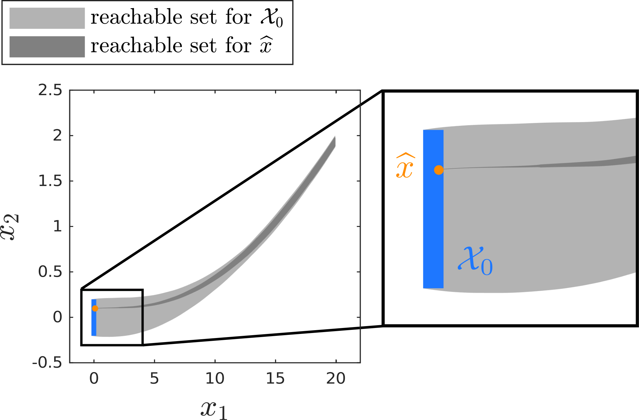
Refer to caption
Figure 9. Visualization of Example 4 with the initial set 𝒳𝟎\mathbf{\mathcal{X}_{0}} and the measured state x^\widehat{x}.
Example 0.

We consider the example of the turn-left maneuver of an autonomous car from (Schürmann and Althoff 2017, Sec. 6) with the measured velocity v^=20.2​ms\widehat{v}=20.2\frac{m}{s}, the measured orientation ϕ^=0.01​r​a​d\widehat{\phi}=0.01rad, and the measured position x^1=0.1​m\widehat{x}_{1}=0.1m, x^2=0.1​m\widehat{x}_{2}=0.1m. The reachable set for the initial set 𝒳0\mathcal{X}_{0} and reachable set extracted for then measured point x^=[v^​ϕ^​x^1​x^2]T\widehat{x}=[\widehat{v}~\widehat{\phi}~\widehat{x}_{1}~\widehat{x}_{2}]^{T} is visualized in Fig. 9. As shown in Table 2, the extraction of the reachable set for the measured point from the offline-computed reachable set is significantly faster than the computation of the reachable set using Alg. 1.

5. Conclusion

In this paper, we showed that the computation of the reachable set for nonlinear systems with the conservative polynomialization approach using polynomial zonotopes preserves the dependence between the reachable states and the initial states. Since this novel method supports the efficient computation of reachable subsets inside pre-computed reachable sets, many possible applications are opening up. For the three applications safety falsification, optimization over reachable sets, and motion-primitive based control we demonstrated with numerical examples that using our novel method results in significant speed-ups compared to the previous solutions. Besides, our method for extracting reachable subsets has complexity 𝒪⁡(n2)\mathcal{O}(n^{2}) and is therefore computationally much more efficient than to compute the reachable subset from scratch, which has complexity 𝒪⁡(n5)\mathcal{O}(n^{5}). Furthermore, this paper provides to some extent a method for unifying reachability analysis and falsification.

Acknowledgements.
The author gratefully acknowledges financial support from the German Research Foundation (DFG) project faveAC under grant number AL 1185/5-1.

References

  • (1)
  • Althoff (2013) M. Althoff. 2013. Reachability Analysis of Nonlinear Systems using Conservative Polynomialization and Non-Convex Sets. In Hybrid Systems: Computation and Control. 173–182.
  • Althoff (2015) M. Althoff. 2015. An Introduction to CORA 2015. In Proc. of the Workshop on Applied Verification for Continuous and Hybrid Systems. 120–151.
  • Althoff and et al. (2008) M. Althoff and et al. 2008. Reachability Analysis of Nonlinear Systems with Uncertain Parameters using Conservative Linearization. In Proc. of the 47th IEEE Conference on Decision and Control. 4042–4048.
  • Annapureddy and et al. (2011) Y. Annapureddy and et al. 2011. S-TaLiRo: A Tool for Temporal Logic Falsification for Hybrid Systems. In Proc. of Tools and Algorithms for the Construction and Analysis of Systems. 254–257.
  • Asarin and et al. (2007) E. Asarin and et al. 2007. Hybridization Methods for the Analysis of Nonlinear Systems. Acta Informatica 43 (2007), 451–476.
  • Bak and Duggirala (2017a) S. Bak and P. S. Duggirala. 2017a. HyLAA: A Tool for Computing Simulation-Equivalent Reachability for Linear Systems. In Proc. of the 20th International Conference on Hybrid Systems: Computation and Control. 173–178.
  • Bak and Duggirala (2017b) S. Bak and P. S. Duggirala. 2017b. Simulation-Equivalent Reachability of Large Linear Systems with Inputs. In Proc. of International Conference on Computer Aided Verification. 401–420.
  • Benvenuti and et al. (2014) L. Benvenuti and et al. 2014. Assume-guarantee verification of nonlinear hybrid systems with ARIADNE. International Journal of Robust and Nonlinear Control 24 (2014), 699–724.
  • Bogomolov and et al. (2019a) S. Bogomolov and et al. 2019a. Falsification of hybrid systems using symbolic reachability and trajectory splicing. In Proceedings of the 22nd ACM International Conference on Hybrid Systems: Computation and Control. ACM, 1–10.
  • Bogomolov and et al. (2019b) Sergiy Bogomolov and et al. 2019b. JuliaReach: a toolbox for set-based reachability. In Proceedings of the 22nd ACM International Conference on Hybrid Systems: Computation and Control. ACM, 39–44.
  • Chen and et al. (2012) X. Chen and et al. 2012. Taylor Model Flowpipe Construction for Non-linear Hybrid Systems. In Proc. of the 33rd IEEE Real-Time Systems Symposium.
  • Chen and et al. (2013) X. Chen and et al. 2013. Flow*: An Analyzer for Non-Linear Hybrid Systems. In Proc. of Computer-Aided Verification (LNCS 8044). Springer, 258–263.
  • Chen et al. (2014) X. Chen, S. Sankaranarayanan, and E. Ábrahám. 2014. Under-approximate flowpipes for non-linear continuous systems. In 2014 Formal Methods in Computer-Aided Design (FMCAD). IEEE, 59–66.
  • Chutinan and Krogh (2003) A. Chutinan and B. H. Krogh. 2003. Computational Techniques for Hybrid System Verification. IEEE Trans. Automat. Control 48, 1 (2003), 64–75.
  • Dang and et al. (2010) T. Dang and et al. 2010. Accurate Hybridization of Nonlinear Systems. In Hybrid Systems: Computation and Control. 11–19.
  • Duggirala and et al. (2015) P. S. Duggirala and et al. 2015. C2E2: A verification tool for stateflow models. In International Conference on Tools and Algorithms for the Construction and Analysis of Systems. Springer, 68–82.
  • Duggirala and Viswanathan (2016) P. S. Duggirala and M. Viswanathan. 2016. Parsimonious, Simulation Based Verification of Linear Systems. In Proc. of International Conference on Computer Aided Verification. 477–494.
  • Frehse and et al. (2011) G. Frehse and et al. 2011. SpaceEx: Scalable Verification of Hybrid Systems. In Proc. of the 23rd International Conference on Computer Aided Verification (LNCS 6806). Springer, 379–395.
  • Girard and et al. (2006) A. Girard and et al. 2006. Efficient Computation of Reachable Sets of Linear Time-Invariant Systems with Inputs. In Hybrid Systems: Computation and Control (LNCS 3927). Springer, 257–271.
  • Girard and Le Guernic (2008) A. Girard and C. Le Guernic. 2008. Efficient Reachability Analysis for Linear Systems using Support Functions. In Proc. of the 17th IFAC World Congress. 8966–8971.
  • Goubault and Putot (2015) E. Goubault and S. Putot. 2015. A zonotopic framework for functional abstractions. Formal Methods in System Design 47, 3 (2015), 302–360.
  • Goubault and Putot (2019) Eric Goubault and Sylvie Putot. 2019. Inner and outer reachability for the verification of control systems.. In HSCC. 11–22.
  • Hoefkens and et al. (2001) J. Hoefkens and et al. 2001. Scientific Computing, Validated Numerics, Interval Methods. Springer, Chapter Verified High-Order Integration of DAEs and Higher-Order ODEs, 281–292.
  • Immler (2015) F. Immler. 2015. Tool Presentation: Isabelle/HOL for Reachability Analysis of Continuous Systems. In Proc. of the 2nd Workshop on Applied Verification for Continuous and Hybrid Systems. 180–187.
  • Immler and et al. (2019) F. Immler and et al. 2019. ARCH-COMP19 Category Report: Continuous and Hybrid Systems with Nonlinear Dynamics. In ARCH19. 6th International Workshop on Applied Verification of Continuous and Hybrid Systems.
  • Kochdumper and Althoff (2019) N. Kochdumper and M. Althoff. 2019. Sparse Polynomial Zonotopes: A Novel Set Representation for Reachability Analysis. arXiv preprint arXiv:1901.01780 (2019).
  • Kong and et al. (2017) H. Kong and et al. 2017. Safety verification of nonlinear hybrid systems based on invariant clusters. In Proceedings of the 20th International Conference on Hybrid Systems: Computation and Control. ACM, 163–172.
  • Kurzhanski and Varaiya (2000) A. B. Kurzhanski and P. Varaiya. 2000. Ellipsoidal Techniques for Reachability Analysis. In Hybrid Systems: Computation and Control (LNCS 1790). Springer, 202–214.
  • Li and et al. (2018) M. Li and et al. 2018. Safe over-and under-approximation of reachable sets for autonomous dynamical systems. In International Conference on Formal Modeling and Analysis of Timed Systems. Springer, 252–270.
  • Liu and et al. (2011) J. Liu and et al. 2011. Computing semi-algebraic invariants for polynomial dynamical systems. In Proceedings of the ninth ACM international conference on Embedded software. ACM, 97–106.
  • Makino and Berz (2009) K. Makino and M. Berz. 2009. Rigorous Integration of Flows and ODEs using Taylor Models. In Proc. of Symbolic-Numeric Computation. 79–84.
  • Matringe and et al. (2010) N. Matringe and et al. 2010. Generating invariants for non-linear hybrid systems by linear algebraic methods. In International Static Analysis Symposium. Springer, 373–389.
  • Mitchell and et al. (2005) I. M. Mitchell and et al. 2005. A Time-Dependent Hamilton–Jacobi Formulation of Reachable Sets for Continuous Dynamic Games. IEEE Trans. Automat. Control 50 (2005), 947–957.
  • Prabhakar and Viswanathan (2011) P. Prabhakar and M. Viswanathan. 2011. A Dynamic Algorithm for Approximate Flow Computations. In Hybrid Systems: Computation and Control. 133–142.
  • Ray and Gurung (2015) R. Ray and A. Gurung. 2015. Parallel state space exploration of linear systems with inputs using XSpeed. In Proceedings of the 18th International Conference on Hybrid Systems: Computation and Control. ACM, 285–286.
  • Sandretto and Chapoutot (2016) Julien Alexandre Dit Sandretto and Alexandre Chapoutot. 2016. DynBEX: a Differential Constraint Library for Studying Dynamical Systems.
  • Schupp and et al. (2017) Stefan Schupp and et al. 2017. HyPro: A C++ library of state set representations for hybrid systems reachability analysis. In NASA Formal Methods Symposium. Springer, 288–294.
  • Schürmann and Althoff (2016) B. Schürmann and M. Althoff. 2016. Closed-Form Expressions of Convex Combinations for Controller Design. In Proc. of American Control Conference. 2795–2801.
  • Schürmann and Althoff (2017) B. Schürmann and M. Althoff. 2017. Convex Interpolation Control with Formal Guarantees for Disturbed and Constrained Nonlinear Systems. In Proc. of Hybrid Systems: Computation and Control. 121–130.