Single Pulse Detection Algorithms for Real-time Fast Radio Burst Searches using GPUs
Abstract
The detection of non-repeating or irregular events in time-domain radio astronomy has gained importance over the last decade due to the discovery of fast radio bursts. Existing or upcoming radio telescopes are gathering more and more data and consequently the software, which is an important part of these telescopes, must process large data volumes at high data rates. Data has to be searched through to detect new and interesting events, often in real-time. These requirements necessitate new and fast algorithms which must process data quickly and accurately. In this work we present new algorithms for single pulse detection using boxcar filters. We have quantified the signal loss introduced by single pulse detection algorithms which use boxcar filters and based on these results, we have designed two distinct ”lossy” algorithms. Our lossy algorithms use an incomplete set of boxcar filters to accelerate detection at the expense of a small reduction in detected signal power. We present formulae for signal loss, descriptions of our algorithms and their parallel implementation on NVIDIA GPUs using CUDA. We also present tests of correctness, tests on artificial data and the performance achieved. Our implementation can process SKA-MID-like data 266 faster than real-time on a NVIDIA P100 GPU and 500 faster than real-time on a NVIDIA Titan V GPU with a mean signal power loss of . We conclude with prospects for single pulse detection for beyond SKA era, nanosecond time resolution radio astronomy.
Keywords — FRB — Transient detection — Astronomy data reduction — Computational astronomy — Single pulse detection — GPU — CUDA
1 Introduction
The discovery of Fast Radio Bursts (FRBs) by Lorimer et al., 2007 and Rotating Radio Transients (RRATs) by McLaughlin et al., 2006 has highlighted the importance of single pulse detection in time-domain radio astronomy. FRBs and RRATs are rare, non repeating or irregular events, therefore their accurate detection is of great importance if we are to understand the nature of the objects producing them. Furthermore, on modern radio telescopes the algorithms for single pulse detection are required to process more and more data collected by these instruments. Also, the rise of multiwavelength astronomy which requires real-time or near-real-time (Middleton et al., 2017) detections increases the requirements put on single pulse detection even more. All of this necessitates the need for fast and accurate algorithms designed to detect single isolated pulses. Single pulse detection algorithms are of importance in searches for giant pulses or irregular pulses from nulling pulsars also.
The single pulse search was described by Cordes and McLaughlin, 2003 as an exercise in matched filtering. They employed a set of boxcar filters of widths . This technique was used successfully in subsequent works (for example Cordes et al., 2006, Deneva et al., 2009, Burke-Spolaor and Bailes, 2010, Rubio-Herrera et al., 2013). The boxcar filter approach was also adopted by many software packages, like Heimdall11 1 https://sourceforge.net/projects/heimdall-astro/, Seek22 2 https://github.com/SixByNine/psrsoft, Destroy33 3 https://github.com/evanocathain/destroy_gutted. In some cases it is beneficial to use more targeted matched filters as suggested by Keane et al., 2010.
The single pulse detection problem is also being explored using machine learning and deep learning techniques for example Wagstaff et al., 2016, Zhang et al., 2018, Connor and van Leeuwen, 2018. Comparison of these techniques to traditional searches is however outside the scope of this work.
It is becoming increasingly important to understand the associated sensitivity and signal loss introduced by algorithms and software when considering the overall performance of a radio telescope. As such, any sensitivity loss introduced by algorithms or software must be investigated. This was discussed by Keane and Petroff, 2015, where the authors compared the sensitivity of different single pulse detection algorithms. Single pulse detection algorithms can have many different forms all with different sensitivities, and also different computational costs. In the case of single pulse detection by boxcar filters, the decrease in sensitivity can occur when a detected pulse is poorly matched by the filters used to extract it from the noise in which it is embedded.
In this work, we quantify sources of signal loss which occur when single pulses are detected using boxcar filters. Based on these, we have designed two distinct methods to distribute and create a limited set of boxcar filter widths in such a way that the signal loss is controlled. We show that the methods presented significantly increase the computational efficiency of traditional approaches and hence provide a significant reduction in execution time, which is of relevance to real-time processing pipelines. We present formulae for calculating the signal loss introduced by a given set and distribution of boxcar filters for an idealized model which uses rectangular pulses. These formulae allow the user to tune the signal loss of their single pulse detection scheme. We present calculations of the computational complexity and the number of memory accesses associated with each method.
Based on our two methods we have designed and implemented two single pulse detection algorithms for NVIDIA GPUs. These algorithms rely on reusing partial sums to calculate long boxcar filters required for detection of wide single pulses. This increases computational efficiency and decreases the number of memory accesses. We present optimization techniques used in the implementation of these algorithms on GPUs. We also describe the advantages and disadvantages of these algorithms. Reusing partial sums to increase computational efficiency is well known in the radio astronomy community. It has been successfully used in the fast folding algorithm by Staelin, 1969 with the most recent implementation by Parent et al., 2018 (using python). The reuse of partial sums was also successfully used in the tree de-dispersion algorithm by Zackay and Ofek, 2017 who implemented tree de-dispersion using CPU, but also suggested an algorithm suitable for GPUs.
This work is part of the AstroAccelerate software package Armour et al., 2019, a GPU optimized time-domain processing pipeline for radio astronomy data. It contains GPU implementations of common signal processing tools used in time-domain radio astronomy, such as de-dispersion by Armour et al., 2012b, a GPU implementation of the Fourier domain acceleration search by Dimoudi et al., 2018, and also periodicity search with a GPU implementation of the harmonic sum by Adámek and Armour, 2018. Aspects of the work have been used in Karastergiou et al., 2015 and Mickaliger et al., 2018.
This paper is structured as follows. First, in section 2 we analyze the sensitivity of the single pulse detection method which uses boxcar filters and derive formulae for quantifying the signal loss. In section 3 we present two distinct algorithms and describe their implementation using the CUDA language extension on NVIDIA GPUs. Our results are presented in section 4, where we present sensitivity of our algorithm when applied to rectangular, Gaussian and double Gaussian pulse profiles with and without white noise. We prove the correctness of our implementation by comparing the measured signal loss with predicted values. We also present the performance of both algorithms and compare it to Heimdall, a GPU accelerated pipeline by Jameson and Barsdell, 2018, Barsdell et al., 2012. We conclude the paper in section 5.
2 Single pulse detection
The aim of the single pulse search, which represents a whole set of techniques and methods, is to find isolated pulses in input data. In this work we focus on the step responsible for recovering the pulse, located somewhere in the input time-series. We will refer to this step as single pulse detection or the SPD algorithm.
Single pulse detection, in general, relies on a match filtering process, which is a convolution of the input time-series with a response function . Convolution in the time domain is given by
| (1) |
where is the time sample, is the filtered time-series and is the length of the response function. The response function is typically designed to detect pulses of a certain or similar shape of width . Significantly longer pulses of the same shape or of different shape require a different response function . A Matched filtering approach thus requires multiple passes through the data in order to cover the desired range of widths and shapes and the convolution is computationally expensive and offers little opportunity to reuse data44 4 This is because partial sums from which we can construct the output sample cannot be used to construct sample , since the elements of within these sums are weighted by the matched filter ..
Because of the computational expense of matched filtering, we have decided to use boxcar filters for our single pulse detection algorithm. If we assume that the pulse we would like to detect could be located anywhere within the time-series, be of any shape, and have a wide range of widths, the boxcar filter is a viable alternative. Boxcar filters are less sensitive than matched filters, but offer two important advantages over the matched filter approach. They are independent of the pulse shape and they allow us to reuse data and computations, which is critical when producing an algorithm for execution on modern computer architectures, especially accelerator architectures such as GPUs.
The boxcar filter is a simple running sum which can be expressed as
| (2) |
where is the boxcar width. This formalism allows us to reuse partial sums because we can form a new longer boxcar filter from an appropriate combination of shorter boxcar filters.
We can measure the strength of a sample by calculating the signal-to-noise ratio (SNR). The SNR of the -th sample from a time-series is calculated by the formula
| (3) |
where , is the mean and standard deviation of the underling noise in the initial time-series . By applying a boxcar filter to a time-series we are creating a new time-series with different mean and standard deviation . The SNR for a pulse from this time-series is then calculated as
| (4) |
where is given by equation (2). The value of the new time-series is a value of the boxcar filter and the bin width, or put another way, the number of the accumulated samples from the initial time-series is equal to the boxcar width.
We have chosen to adopt the SNR of the pulse as a figure of merit by which we measure how well any SPD algorithm detects individual pulses.
The SNR produced by the algorithm which we call recovered SNR (RSNR), to distinguish it from the true SNR of the pulse, is calculated using equation (4). The value of the RSNR depends not only on the initial SNR of the injected pulse and its shape, but also on its position within the time-series and its width. This is because to localize the pulse and sum the power contained within it, we use an incomplete set of boxcar filters. That is, the boxcar filters do not cover every possible pulse width at every possible time sample. As a consequence a pulse of the same shape could be detected with different based on its position in time and its width. Lower occurs when the injected pulse is not properly matched by these filters either in width or position in time. The highest will be produced by the boxcar with width and position that best fits the unknown signal.
2.1 Idealized signal model
In order to compare algorithms, to evaluate sensitivity loss and to simplify sensitivity analysis, we have introduced an idealized model (simplified toy model) of the input signal.
The simplest form of signal which fits this role is the signal with a rectangular pulse, without any noise, where all samples except those of the pulse are set to zero. The pulse is described by its position within the time-series, by its width , and by its amplitude . The mean () and standard deviation () which are required in the calculation of the SNR (eq. (3)) are set to and to simulate the presence of white noise.
To get the value of the mean and standard deviation for longer boxcar filters we use the white noise approximation. That is the mean and standard deviation for time-series after application of the boxcar filter of width is given as
| (5) | ||||
For the white noise approximation we get and .
For the purpose of comparing the sensitivity of the SPD algorithm to different pulse widths we normalize the amplitude () of the rectangular pulse to
| (6) |
where is a normalization constant. The normalization ensures that the RSNR produced by the boxcar filter which fits the rectangular pulse perfectly is the same regardless of the pulse width .
2.2 Sensitivity analysis
We quantify the sensitivity of the SPD algorithm in terms of signal loss. The signal loss is given as the fraction of the pulse’s true () which was not detected by the algorithm. That is, the difference between RSNR detected by the algorithm and the true value of the injected pulse divided by ,
| (7) |
where the value of depends on the pulse width, width of the boxcar filter used for detection and on the position of the boxcar filter with respect to the pulse’s position.
As the position of the signal is unknown we must apply the boxcar filter of width to the whole time-series , which may or may not by applied to each and every time sample. If we are only interested in the highest detected, for fixed boxcar width , then this reduces the sensitivity analysis to a problem of two consecutive boxcar filters separated by time samples, we call this distance boxcar separation. This problem which is depicted graphically in Figure 1 is then repeated throughout the whole time-series . This allows us to avoid studying individual boxcar filters, but still gives enough flexibility to evaluate sensitivity or signal loss introduced by the SPD algorithm for any signal present in the time-series.

In our analysis of the sensitivity of SPD algorithms, for a detailed description see appendix A, we have, using the idealized signal model, identified two quantities of the which can be used to describe the sensitivity of an SPD algorithm.
The first is the lowest RSNR detected by the SPD algorithm under the worst conditions given the pulse width . This acts as an infimum (greatest lower bound) for detected by the SPD algorithm for any pulse of a given width . Along with it, we define worst case scenario signal loss
| (8) |
that is the greatest signal loss introduced by the SPD algorithm.
The second quantity is the highest possible value of RSNR () which could be recovered by the SPD algorithm under the best possible circumstances for the given pulse width . This acts as a supremum (least upper bound) for which could be detected by the SPD algorithm. To accompany this quantity we have defined the systematic signal loss
| (9) |
which is always introduced by the SPD algorithm for a pulse of width .
2.2.1 Parameters of the SPD algorithm
We have also determined two parameters which describe the SPD algorithm and have direct implication on the sensitivity. We characterize the SPD algorithm by the set of boxcar filter widths and by boxcar separation for each boxcar width .
The number of different boxcar widths, that is the sparsity of the set affects the value of . We can increase (decrease the systematic signal loss ) by including more boxcar filter widths performed by the SPD algorithm. The set to a lesser degree also affects .
The value of the boxcar separation is most important for the value of . In order to increase (decrease the worst case signal loss ) we have to decrease the boxcar separation .
The SPD algorithm may consist of multiple iterations where both and may differ. We assume that the time-series in which we want to detect pulses is completely covered by boxcar filters of a given width .
2.2.2 Importance of maximum and minimum RSNR
There are several reasons why is important. Firstly, from surpremum and infimum properties of the we get . That is, we cannot increase above . Since is mainly improved by decreasing boxcar separation this means that decreasing may yield diminishing results. This is shown in Figure 2.

Secondly, the gives a hint at how we can increase or decrease the sensitivity of an algorithm, but also how to trade sensitivity for computational performance.
Lastly, by knowing for a given SPD algorithm we can compare them and rank them. It can also serve as a verification tool to check if an implementation of a given algorithm works as expected. In this case the algorithm must not produce any RSNR value which would lie outside the limits given by .
2.2.3 Error in detected pulse width and time
The error in the detected width of the pulse for the SPD algorithm can be expressed as
| (10) |
where is the true pulse width and is the boxcar width which has detected the pulse, i.e. the detected width.
Similarly we can define the error in detected position in time relative to its true position (time localization) as a fraction of its true width as
| (11) |
where is the true pulse position in time and is the boxcar time position.
3 Single pulse detection algorithms
The single pulse detection algorithm may be required to scan for very long pulse widths with related maximum boxcar filter width . This could lead to unnecessary precision and longer execution time as more boxcar filters than it is necessary would be calculated. This is why both of our proposed SPD algorithms execute in multiple iterations with different parameters and inputs. This allows us to control precision and increase performance. In order to decrease the sensitivity of the SPD algorithm and to lower the amount of data which are processed we use decimation in time (by a factor ).
To distinguish quantities from different iterations we decorate them with an index , starting with . We assume for simplicity that the decimation factor does not change during the execution of the algorithm and means to the power of and not an iteration index. Thus we have:
- •
input time-series for given iteration ( is the initial time-series)
- •
a set of boxcar widths used in th iteration
- •
is the value of the boxcar filter for width at time sample
- •
is the value of the boxcar filter at the end of iteration
- •
is the maximum desired pulse width to be searched for
- •
is the maximum boxcar width calculated by the SPD algorithm; is the boxcar width of the nearest longer boxcar filter to the value of
The output of the SPD algorithm is the highest RSNR value detected by the boxcar filters. We have chosen to separate the output by iteration, that is the output for th iteration is
| (12) |
where the SNR value is calculated using equation (4). In addition to the SNR value we assume that the SPD algorithm provides the width of the boxcar which produced the highest SNR value .
When designing an algorithm that is suitable for execution on GPUs, it is important to have enough parallelism to ensure high utilization of the GPU hardware. Modern GPUs can process many thousands of threads concurrently. The memory available for a single thread on the GPU is extremely limited, either in the form of registers or the amount of shared memory available. Therefore cooperation between threads within a single threadblock55 5 Threadblock is a set of threads that can cooperate with each other. is important. The amount of resources (for example the amount of local memory) consumed by a threadblock and how many threadblocks can be executed concurrently then depends on the number of threads per threadblock.
3.1 BoxDIT algorithm
The algorithm we call BoxDIT is based on the ideal SPD algorithm. The ideal SPD algorithm is the algorithm that performs boxcar filters of all widths up to a maximum at each element of the initial time-series, thus detects any rectangular pulse with with its true SNR value. The ideal SPD algorithm has poor performance due to unnecessary high sensitivity. The BoxDIT algorithm trades some sensitivity for performance by introducing the decimation step which reduces the number of boxcar filter widths performed and increases boxcar separation .
The BoxDIT algorithm (algorithm 1) is a sequence of iterations, where each iteration has two steps. The first step is to perform all boxcar filters up to with respect to time-series , at every point of the input data . From the perspective of the initial time-series the algorithm calculates boxcar filters with a width step at every point of the initial time-series. For example, if for all then: boxcar filters of width are calculated at every point; after decimation, boxcar filters of width are calculated at every second point and so on. Thus, each subsequent iteration detects wider pulses in the input data. This step uses the previously calculated boxcar filter data to calculate longer boxcar filters.
The second step is to decimate the time-series in time by a factor to create time-series for the next iteration. This is repeated until is reached. The decimation in time that is used in this paper is given by
| (13) |
for all . That is, the th element of the decimated time-series is set to a position of the next time sample which must be added to the partial sum containing th element of the initial time-series . This is shown in Figure 3. Such a decimation has the advantage that the maximum width performed at any iteration of the BoxDIT algorithm has to fulfil only the condition that it is divisible by . During the decimation step we also reduce the number of time samples to , this is important as the higher iterations work with fewer points. Thus each BoxDIT iteration is characterized only by and .
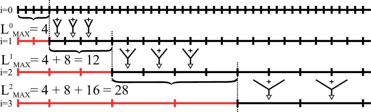
The width of the boxcar filter calculated by iteration is given as
| (14) |
This could be also used to calculate the maximum boxcar width for given iteration .
The value of the boxcar filter at time sample for iteration is given as
| (15) |
where .
The advantage of the BoxDIT algorithm is that the sensitivity of the algorithm is easily adjusted by changing the maximum boxcar width calculated by the boxcar step of the algorithm. The disadvantage of the BoxDIT algorithm is that it has higher memory bandwidth requirements since in addition to the decimated input data it also needs the values of the longest boxcar filter at every point, which in effect doubles the size of the input data.
3.1.1 BoxDIT GPU implementation
The GPU implementation of the BoxDIT algorithm performs both steps, calculation of boxcar filters and decimation, in one GPU kernel. The implementation must be able to extend the already calculated boxcar filters by using values from the previous iteration. Such an implementation can be used for any iteration of the BoxDIT algorithm without change.
On the input, we have the time-series , values for the longest boxcar filter from the previous iteration , and maximum boxcar width calculated in this iteration. On the output we expect to have the highest RSNR for every point of the input time-series, associated boxcar width , values of the longest boxcar calculated and decimated time-series for next iteration . We have used the decimation factor for the GPU implementation of BoxDIT.

Calculating all boxcars up to given maximum width at a given point is equivalent to performing a prefix sum or a scan. In this case, the scan has to be performed at every point of the input time-series. We have found that using the standard prefix sum algorithm like the Hillis-Steel scan Hillis and Steele, 1986 to be slow even when used on cached data. The reason is that series independent scan operations do not cooperate by reusing data enough. Our implementation focuses on increased cooperation between independent prefixed sums within the GPU thread-block.
The pseudo-code for the parallel GPU implementation of the BoxDIT algorithm is given in Algorithm 2 and a graphical sketch is presented in Figure 4. This figure shows how we divide work among GPU threads and how threads cooperate on a calculation of independent prefixed sums.
As a first step, each thread calculates a much shorter prefixed sum of length . That is each thread calculates partial sums , where is a time sample and is the length of the partial sum in the number of time samples. These partial sums are stored into the GPU registers66 6 GPU registers are the fastest type of GPU memory, but private to an individual thread. of a given thread. These partial sums serve as accumulators used for calculation of the longer partial sums. The value of the last partial sum is also stored into shared memory77 7 Shared memory is a fast user managed cache on the GPU which all threads in a thread block can access., because its value has to be distributed among other threads. The maximum SNR for a given time sample and boxcar width are also stored in the shared memory as they will be modified by other threads.
After this initial phase, each thread reads the partial sum from its appropriate place in shared memory. Then using accumulators stored in its registers (partial sums , for ) each thread is able to produce a prefixed sum up of length . That is partial sums , where . These partial sums are calculate as
| (16) |
The accumulators in the threads registers are then updated to the new values representing partial sums . The thread calculates SNR value for each accumulator and compares it to the highest detected SNR for a sample . If the new SNR is higher than the old SNR, the highest SNR is updated together with boxcar width .
With each following iteration, each thread calculates longer partial sums for time samples which are further from its starting time samples.
The number of iterations required to calculate all required boxcars is . The algorithm used in our implementation can be expressed by equation
| (17) |
where .
At the last step of the algorithm, the maximum values of the SNR , the boxcar width and the longest accumulated partial sum representing the value of the boxcar filter of width are stored into the device memory.
The intermediate partial sums produced by the algorithm are not stored to device memory as they are needed only for finding the maximum SNR for every input sample.
3.2 IGRID algorithm
Our second algorithm, which we call IGRID, is based on the decimation in time SPD algorithm (DIT algorithm). The DIT algorithm has poor sensitivity, with the average signal loss of and the worst signal loss of , but it has high performance. In terms of both are low. The IGRID algorithm decreases signal loss at the expense of the performance.
The DIT algorithm, shown in Algorithm 3, is a sequence of decimations in time applied repeatedly on the input time-series , thus in effect producing boxcar filters of width , where is the number of decimations performed so far. Therefore we have , where is the total number of iterations performed. The distance between these boxcar filters is the same as the width . Based on our analysis in section 2 we can say that large values of are mostly responsible for low values, while sparse coverage of boxcar widths are responsible for low values. The IGRID algorithm corrects for these shortcomings.

One way of decreasing is to perform an additional DIT operation on the input data producing additional time-series , which is shifted by one sample ( samples from the perspective of the initial data). That is for initial time-series we would create one more time-series in addition to the already existing time-series which results from DIT operation which was not shifted. Let’s call these decimated time-series layers and decorate them with a subscript indicating their shift in the number of samples with regard to the initial time-series . That is is a layer in the iteration with the shift . Let’s also introduce IGRID step which is a set of layers with different shifts but with the same decimation.
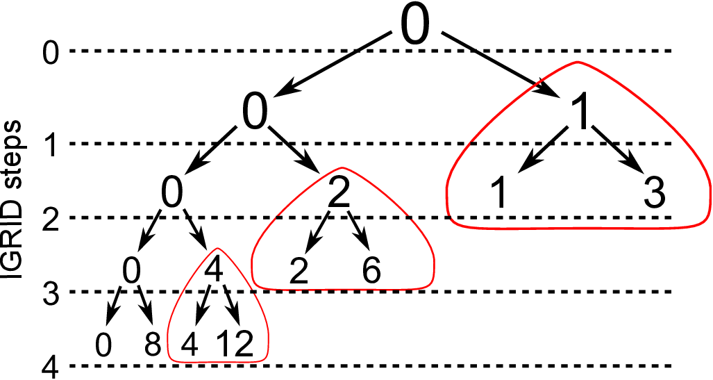
In general if we have a parent layer which is decimated by times, that is each sample is a sum of samples from the initial time-series , we can use it to calculate two new child layers, one layer with the same shift as the parent’s and second layer which is shifted by initial time samples compared to the parent. This is shown in Figure 5, where we have:
- •
Layer:
- •
Layer: and
- •
Layer: and note that layers 1 and 3 are not needed for further iterations
In this example, we have chosen not to use layers and . This means the increases, but we do not need to keep these layers in memory and process them in further iterations.
Thus by using layers we can decrease the distance between boxcar filter to . These layers must be shifted by samples in order to have a constant step between each boxcar filter. An uneven distribution of boxcar filters leads to increased signal loss at some parts of the input time-series.
We can look at the algorithm differently using the time shifts alone, which now represent appropriate layers. This is shown in Figure 6. The layer dependencies (from Figure 5) have the structure of a binary tree (for decimation factor ). If we focus on the right branches (marked in red) we see that after a few IGRID steps there are no layers dependent on layers located in these right branches of the binary tree. If we are able to keep and process all layers from these branches in local memory, then all we need to keep in the device memory are layers .

The binary tree structure also hints at how we can deal with the second problem of the DIT algorithm, which is the scarcity of the set of boxcar filter widths . By decreasing we increase but not , which could result in the situation, where cannot increase further since . This is shown in Figure 2.
We can increase the number of calculated widths if we use boxcar filters from previous IGRID steps and add them to boxcar filters from the current IGRID step. In other words, we traverse the binary tree in an upward direction toward the root. The IGRID steps contain boxcar filters of width , thus by using previous IGRID steps we can produce boxcar filters of width
| (18) |
where is depth or the number of previous IGRID steps used, and are variables determining the width of the resulting boxcar filter. The values of are further restricted to for positive and also since smaller boxcars then would be calculated in the previous IGRID step. This means that any given IGRID step, depending on depth can produce any boxcar width . An example of this is shown in table 1 for starting boxcar of width . However, by increasing the depth we increase the number of layers which the IGRID algorithm needs to access and therefore share between IGRID steps. The effect on caused by increasing the set is shown in Figure 7.
| Depth | Width | Increment | |||||||
|---|---|---|---|---|---|---|---|---|---|
| a | 1 | -1 | -1 | 1 | 1 | -1 | 1 | 1 | |
| 0 | 16 | 0 | |||||||
| 1 | 16 | 24 | +8 | ||||||
| 2 | 16 | 20 | 24 | 28 | +4 | ||||
| 3 | 16 | 18 | 20 | 22 | 24 | 26 | 28 | 30 | +2 |
The advantage of the IGRID algorithm is that it has low memory bandwidth requirements (for lower precision) as all data required by the algorithm is contained in the decimated input data . The disadvantage of the IGRID algorithm is that for higher precision we have to use previous IGRID steps which substantially changes the character of the algorithm (more input data, more complicated calculations of boxcar filters). This makes the IGRID algorithm hard to implement in a flexible way.
3.2.1 IGRID GPU implementation
We have implemented the IGRID algorithm with three levels of precision, these are abbreviated as , where is the depth. We have used three depths which corresponds to IGRID algorithms IG(1), IG(2), and IG(3). Each implementation of the IGRID algorithm also uses a different number of layers. We have chosen 4 layers for the IG(1) 8 layers for the IG(2) and 16 layers for the IG(3) algorithm per IGRID step. We have implemented three different precision’s because it allowed us to optimize each case and get the highest performance.
The main problem of the IGRID algorithm, especially when it is performed with a higher depth parameter, is the amount of data which needs to be shared between IGRID steps. For IG(1) we do not need any additional data since the input layer can also be used to calculate wider boxcar filters. However for IG(2) we need in addition to the input layer , also its parent , and finally for IG(3) we need the parents of the parents (). This means that the size of the input data for IG(2) is twice as big as for IG(1) and the size of the input data for IG(3) is four times bigger than that of IG(1). All of this data needs to be read and written by each IGRID step. This would slow down the code considerably and make it memory bandwidth bound.
In our implementation of the IGRID algorithm we have chosen to process more than one IGRID step per one execution of the GPU kernel. Algorithm 4 describes how the IGRID steps are split into blocks. Processing more IGRID steps per GPU kernel is beneficial in a number of different ways. If we perform more IGRID steps together we not only remove device memory accesses between individual IGRID steps, but we also reduce the amount of data shared between consecutive GPU kernel executions, since each IGRID step reduces the amount of data by half due to decimation in time. The data shared between IGRID steps within one GPU kernel execution are stored in GPU shared memory.
The second benefit comes when we process whole right branches which are marked in Figure 6. As discussed above, each right branch depends only on the layer with zero shift, but in order to calculate whole IGRID step we might need layers from different branches. That is demonstrated by IGRID with a step of two in Figure 6. We see that, to calculate a whole step, we need layers with shifts , but layers with shifts and are from different branches. If we do not calculate the entire right branch within one execution we would have to save all or some of the intermediate data to the device memory.
Therefore we have chosen to calculate whole sub-sections of the binary tree starting always at the layer with zero shift and going down to a chosen depth, even if it means calculating parts of the tree which are later discounted. Recalculating parts of the binary tree allows us to save device memory bandwidth and increases the performance in the process. This is shown in Figure 8. The other indirect benefit is that we can achieve higher sensitivity, since we calculate parts of the tree which would not be calculated otherwise.
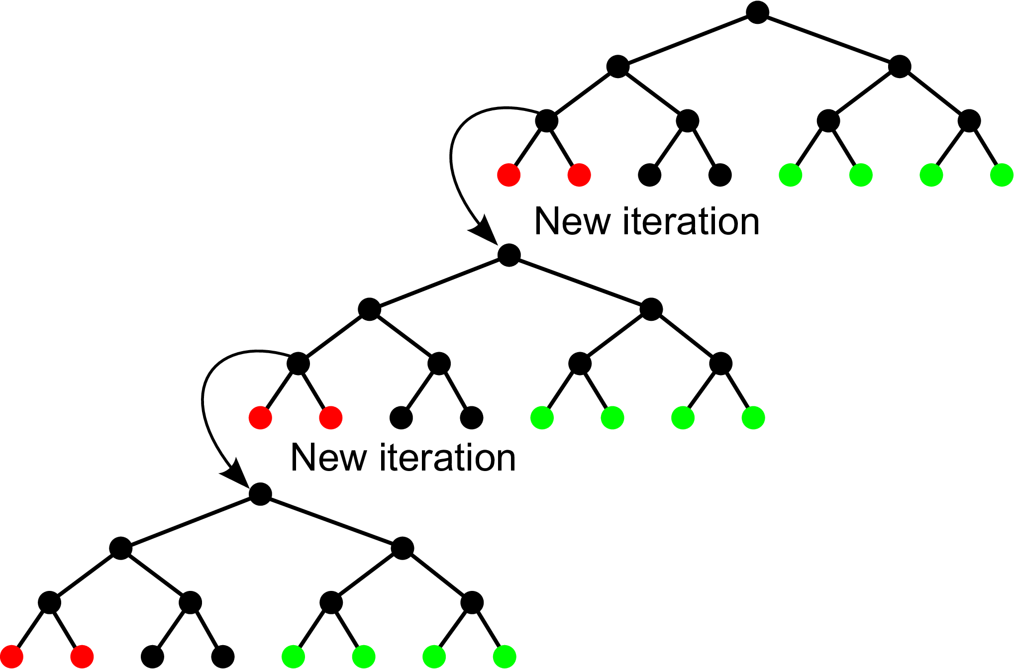
The calculation of the binary tree itself inside the GPU kernel exploits the property of decimation in time, where the output decimated time-series is half the size of the input. After decimation we are able to fit two decimated layers into the memory space instead of one. The process of calculating these two child layers from the parent layer can be performed in one operation. If we use a running sum of size two (a boxcar filter of width two) we can calculate the two child layers in-place but they will be mixed together, one in even samples, the second in odd samples. Figure 9 depicts how this calculation of a sub-section of the binary tree is performed. As we perform more decimations we can fit more layers into the same memory space but also the individual layers are more intertwined as we see in Figure 9 for later IGRID steps.

The GPU kernel uses shared memory to calculate these decimations. A thread which performs the boxcar filter of width two has to add the sample with increasing step, in order to use samples from the correct layer. Each thread always writes into the same memory address. Thus during the calculation a thread calculates time samples from different layers as is shown in Figure 5, where, for example, the 7th thread calculates 8th time sample from the zero shifted layer, then the 4th time sample from the layer which is shifted by one sample and so on. Accesses to shared memory are without bank conflicts. The algorithm for IG(2) is shown in Algorithm 5.
3.3 Computational and memory complexity
The number of operations and number of memory accesses of one iteration for both proposed algorithms is summarised in table 2.
| Algorithm | # floating | # global |
|---|---|---|
| point operations | memory accesses | |
| Ideal boxcar filter | ||
| Decimation in time | ||
| BoxDIT | ||
| IGRID(IG(1)) |
4 Results
In this section we present a selection of representative configurations for each algorithm and compare them based on performance and signal loss. Implementations presented here assume fp32 floating point numbers for the input.
First we present signal loss for each algorithm and configuration for the idealized signal model (sec. 2.1) using a rectangular pulse. We verify the correctness of our implementation of both algorithms using the idealized signal model by comparing the measured signal loss and (, ) to predicted values of the signal loss and . We also present the error in the detected width of the pulse and the error in the detected position in time relative to its true position (time localization), which are introduced by each algorithm.
Next we present RSNR and error in pulse width and time localization for the idealized signal model with Gaussian and double Gaussian pulse profiles. These pulse shapes are a better approximation of the pulses encountered in real observations.
The recovered SNR and detected width for a rectangular, Gaussian and double Gaussian pulse shapes which are embedded in white noise are presented afterwards. For these results we have used pulses of .
Following this we present the performance of our algorithms on two generations of NVIDIA GPUs, the P100 and the Titan V. The performance of the algorithm is measured in the number of dedispersion trials88 8 A DM trial is a time-series which is the output of the de-dispersion transform algorithm, it corrects for the effects of interstellar medium. (DM trials) which could be performed in real-time for sampling time . We also present the dependency of this number on the maximum width performed by the algorithm.
Lastly we present a comparison of AstroAccelerate with Heimdall and its single pulse search algorithm. We also demonstrate how we calculate mean and standard deviation which is then used for the calculation of recovered SNR.
Results presented here are for three variants of the IGRID algorithm which we have described at beginning of section 3.2.1. To match these three IGRID configurations we chosen three configurations of the BoxDIT algorithm, each with a different ratio of sensitivity and performance. We can change the sensitivity of the BoxDIT algorithm by changing the value of the maximum boxcar width calculated in the boxcar filter step of the algorithm. These configurations are: BD-32 which calculates a maximum width of between decimations for any ; BD-16 with maximum width of ; and BD-8 which uses maximum width of .
4.1 Measurement of signal loss
To measure the signal loss of a given SPD algorithm we have to find the produced by the algorithm and then calculate signal loss using equation (7). The value of depends not only on the SNR of the injected pulse but also on its position within the time-series. This is because to localize the pulse and sum the power it contains, we use an incomplete set of boxcar filters. That is, the boxcar filters do not cover every possible pulse width at every possible time sample. Lower RSNR occurs when the injected pulse is not properly matched by these filters.
Therefore, to accurately measure we have to create data where a pulse of given width will be present in all relevant positions in time. By sliding the pulse along its whole width in time we can evaluate all of these relevant positions for a pulse of a given width. The test data used for the measurement of the consists of a set of time-series where each pulse shift is stored in its own time-series.
The test data are then processed by the SPD algorithm. From each time-series we select the highest RSNR and from these we select the maximum, which is the , and the minimum which is the for a given pulse width.
To evaluate the value of the mean and standard deviation for longer boxcar filters we have used the white noise approximation as discussed in section 2.1 and shown in equation (5).
When we measure the and using our idealised signal model, the pulse will, as slides along its width, be detected by boxcar filters placed at different times. Since we select the first maximum (minimum) we introduce a bias into our measurement of time localization. Meaning that pulses are detected earlier than their true position in time.
When Gaussian noise is present in the test data we must modify how we measure . Since we select the highest SNR for each pulse position, this would prefer pulses which are enhanced by the addition of the noise. Hence, when noise is present we use an averaged from multiple measurements of the pulse’s at the same position. This way we can mitigate the effect of the noise to some degree. Measurement made with noise will always have a tendency to get higher values of , because we select the maximum SNR. For the SNR calculation we have also used the white noise approximation (5).
4.2 Signal loss for idealized signal
The measured and together with measured signal loss (eq. (7)), error in detected width (eq. (10)) and error in time localization (eq. (11)), of the rectangular pulse using our idealized signal model for our chosen configurations of our BoxDIT algorithm are shown in Figure 10 and for our IGRID algorithm in Figure 11. Both errors are expressed as a percentage of the true pulse width.


The error in the time localization shown in Figures 10 and 11 are biased for earlier pulse detection as discussed above.
The comparison to predicted signal loss which is calculated by equations (24) and (31) are shown in figures 10 and 11 as gray and black lines. The measured systematic signal loss must be higher or equal to the predicted , while measured worst signal loss must be lower or equal to the predicted worst signal loss for a given pulse width. In essence any measured value of the must lie be between values for and .
Lastly, in figures 10 and 11, we also present the cumulative average signal loss up to a given pulse width which is calculated as
| (19) |
This represents the mean signal loss one can expect for all pulses with width .
4.2.1 Discussion
The averaged signal loss for our chosen configurations of our BoxDIT algorithm (Fig. 10) ranges from 1% for configuration BD-32 to 3% for configuration BD-8. For IGRID the averaged signal loss starts at 2% for configuration IG(3) and increases to 12.5% for IG(1). The sudden decreases in (increases in signal loss), which occur at different places for different configurations are caused by decimation in time. The decimation in time increases boxcar separation , which in the case of width and time localization determines the time resolution we are able to achieve. The boxcar separation represents the minimum increment in the measured width and the index of the time sample. Thus it is more significant for shorter pulse widths as it is a proportionally bigger part of the pulse’s width. This is why the error in the width and time index decreases with pulse width.
Our IGRID algorithm behaves in a similar way (Figure 11). Our IGRID algorithm has, in general, higher signal loss and a higher error in width and time localization than our BoxDIT algorithm. This is because IGRID places boxcar filters more sparsly than BoxDIT.
A comparison of the measured signal loss and values to the predicted values of the signal loss and for both algorithms is shown on the left in Figure 10 for BoxDIT algorithm and in Figure 11 for IGRID algorithm. Both algorithms give the same values for as is predicted. However both algorithms have better worst signal loss than what is predicted by equation (31). This can be explained in each case. In the case of the IGRID algorithm this is because we calculate more layers than are necessary (section 3.2.1). This results in a smaller signal loss for some pulse widths. For the BoxDIT algorithm the higher is cause by boxcar filters of a shorter width which cover the pulse completely (best case) which has higher RSNR thus lower signal loss than boxcar filters considered in our sensitivity analysis for the worst case.
4.3 Other pulse shapes
The profile of a real signal is usually far from rectangular, this is why we have included results from studies of two other pulse profiles; a Gaussian shape and combination of two Gaussians. We have measured , error in detected width and error in time localization using the idealized signal model. For these alternative pulse shapes we cannot use the equation (7) to calculate signal loss, because these pulses have a non-uniform distribution of power between samples of the pulse. Although the pulse is still normalized to the constant the non-uniform distribution means we can sum most of the pulse power with much shorter boxcar filters which overestimate SNR of the pulse, resulting in higher than .
These pulse shapes are inserted in a similar fashion to the rectangular pulse shape. The input time-series is zeroed - all elements are set to zero. The pulse is then injected at the required position.

To produce these pulses we have sampled the normal distribution given by
| (20) |
where the mean is set to and the variance, , depends on the shape type and width of the pulse. For a Gaussian like shape we have used Brandt, 2014 and for the double Gaussian profile we have used and . The Gaussian profiles are then sampled at discrete intervals to produce values which are then injected into the idealized dataset. These pulses are shown in Figure 12. The signal is normalised such that when all its samples are summed together, i.e. a boxcar of signal width is applied to it, it will produce .
The results for the BoxDIT algorithm in the most sensitive configuration BD-32 are presented in Figure 13. We present results for the fastest configuration of our IGRID algorithm (IG(1)) in Figure 14. We also show an alternative figure of merit to the signal loss in the form of the recovered fraction of a signal’s power in Figure 15 for both algorithms.


4.3.1 Discussion
Figures 13 and 14 show that the of pulse shapes other than rectangular are higher than the maximum for the rectangular pulse. This is due to the non-uniform distribution of power throughout these pulse shapes, where the power is concentrated into fewer samples. This means that a shorter boxcar filter can sum most of the power contained in the pulse which results in a higher RSNR. The fluctuations in for short widths is cause by the poor discreet representation of pulse shapes, shown in Figure 12.
The error in measured width and position in time is presented in figures 13 and 14. We see that boxcar filters systematically under-estimate pulse width when applied to a non-rectangular pulse. The error in the measured width is consistently about of the true pulse width for the single Gaussian and about for double Gaussian. These findings are consistent with the fact that Gaussian like pulse profiles tend to be detected with shorter boxcar filters than their true width due to the non-uniform distribution of power in the pulse.
The error in time localization is presented in figures 13 and 14. Time delay in detection is again expressed as a percentage of the true pulse width. Positive values indicate that the pulse is detected later in time, while negative values indicate that the pulse was detected earlier in time. These results show that Gaussian pulses are detected later than their true position in time. This is also shown in Figure 12 which highlights the portion of the pulse which result in the highest RSNR detection. If we consider a Gaussian pulse that is 20 samples wide we see that it is detected by the boxcar filter with width of 11 samples, centered about the peak. Meaning that the pulse is detected with a time delay of 4 or 5 samples which represents or time delay compared to the true pulse width of 20 samples.
The recovered power by the BoxDIT (BD-32) and IGRID (IG(1)) algorithms for pulses of Gaussian like shapes are presented in Figure 15. We see that to produce the highest for Gaussian like pulses, the algorithm sums on average of the signal’s power or for the double Gaussian pulse profile. These results show that boxcar filters which sum all the power contained within the pulse have lower and thus are not selected as candidates.
The noticeable increase in the width error visible in Figure 14 for the double Gaussian pulse profile as well as the drop in the fraction of recovered power in Figure 15 is because the IGRID algorithm (IG(1)) detects only the first Gaussian out of two that are present in the pulse. The error in time localization, which is unchanged indicates that it is the first Gaussian that is detected. For other configurations of our IGRID algorithm this was not observed. This is because these configurations have a denser set as well as shorter boxcar separation and they are able to better match the entire pulse.
4.4 Time-series with white noise
To verify the results of our SPD algorithms when there is noise present in the input data we have inserted Gaussian noise (mean , standard deviation ) into the idealized signal and measured . To measure we have used the method described in section 4.1. The measured values of for BoxDIT in configuration BD-32 and IGRID in configuration IG(1) are presented in Figure 16. The injected pulses have SNR=16. The effect of the noise on the measured is higher for pulses with lower SNR, as expected.


We have also used time-series with white noise to test SNR extraction. Examples for each pulse shape are presented in Figure 17 for the rectangular pulse, and in Figure 18 for the Gaussian and double Gaussian pulse. The pulses have , width samples and they start at sample 100. For the rectangular pulse, the detection should occur at sample 110 by a boxcar filter of width 20 samples. For other pulse shapes the boxcar width is shorter as shown in Figure 12. The addition of the while noise means that single pulses shown in these figures do not represent overall sensitivity of our algorithms.


4.4.1 Disscusion
The reported by our BoxDIT algorithm in configuration BD-32 and by our IGRID IG(1) algorithm are presented in Figure 16. The introduction of Gaussian white noise into our idealized model with rectangular pulse had only marginal effect on the detected RSNR by both algorithms. This is, for the most part, due to the initial SNR of the injected pulse which was . We also see that produced by both SPD algorithms fluctuate about and often go below . These variations are caused by fluctuations in the detection boxcar’s width and it’s position in time.
Studying other pulse shapes we see that reported by BoxDIT is higher than in case without the noise. This is most visible for the Gaussian pulse shape. This again is due to the pulse shapes having a non-uniform distribution of power in their profile, hence they are detected with shorter boxcar filters than the actual pulse width. This makes it easier for the added noise to change the behavior of the SPD algorithm by changing the distribution of power throughout the pulse. For example, by decreasing the peak in the Gaussian pulse shape the boxcar which detects the pulse will be wider as it needs to accumulate power from more samples and in combination with our normalization this will decrease closer to 16. On the other hand by slightly increasing the peak in pulse profile, the pulse will be detected by a shorter boxcar producing higher .
We see that in the case of the rectangular pulse (fig. 17) the detection occurs at the correct position in time for SNR=8 and SNR=5. For pulse width SNR=3 the highest RSNR is detected at time sample 116 but the detected width underestimates the actual pulse width. This detection is mostly due to noise. The pulse itself is detected correctly at the time sample 110 with width 20, but it has lower RSNR. With decreasing pulse SNR we see that noise has stronger effect on the detected width and position of the pulse as would be expected. The Figure 17 also shows same data in a wider perspective with all candidates above a given threshold. For SNR=3 we see that the injected pulse is detected correctly, however it is hard to distinguish from background noise.
4.5 Performance
We have evaluated the performance of our algorithms and their implementation in different configurations by measuring the execution time. As a derived metric we have calculated the number DM trials that can be searched in real-time using sampling time . Processing data in real-time means performing all of the required operations on the data faster then we acquire the data. The number of DM trials processed in real-time is calculated as ratio of the number of processed time-samples per second by the SPD algorithm and the number of acquired time-samples per second . That is
| (21) |
The number of DM trials processed in real-time depends on the telescope sampling time and for a different sampling time other then , the number of DM trials searched in real-time will be different. For example for the number of DM trials processed in real-time will be multiplied by factor of two .
The number of DM trials searched in real-time also depends on the maximum width of the boxcar filter used for detection of the pulses. In the following results we have used samples, which for a sampling time means a boxcar filter which is approximately half a second long. When searching for shorter pulses, the performance of the SPD algorithm can be increased by using shorter .
We present the performance of our implementations on two NVIDIA GPUs. The first is the TESLA P100 which is a scientific card from the Pascal generation. The second is the Titan V, which is a high end prosumer card from the Volta generation. We have not included any card from the current Turing generation since this generation is not designed for scientific tasks and workloads. The hardware specifications of these two GPUs are summarized in table 3.
| P100 | TITAN V | |
| Total CUDA Cores | 3584 | 5120 |
| Streaming Mul. (SMs) | 56 | 80 |
| Core Clock | 1303 MHz | 1455 MHz |
| Memory Clock | 1406 MHz | 850 MHz |
| Device m. bandwidth | 720 GB/s | 652 GB/s |
| Shared m. bandwidth | 9121 GB/s | 14550 GB/s |
| FP32 performance | 9.3 TFLOPS | 12.3 TFLOPS |
| GPU memory size | 16 GB | 12 GB |
| TDP | 250 W | 250 W |
| CUDA version | 10.1 | 10.1 |
| Driver version | 418.39 | 415.27 |
Execution time and how it scales with increasing number of time-samples (per one DM trial) and execution time scaling with increasing number of DM-trials for the P100 and the Titan V are presented in Figure 19. The calculated number of DM-trials processed in real-time for different sampling times is presented in Figure 20.


The comparison of the two algorithms with respect to their signal loss and achieved performance is presented in Figure 21. This figure combines results presented in Figure 10 and Figure 11 with the number of DM trials processed in real-time using a sampling time . This figure allows us to compare the algorithms signal loss/performance ratio.


Performance as a function of maximum boxcar width searched by the SPD algorithm is presented in Figure 22. In the case of IGRID algorithm, these results depend on how many IGRID steps we perform per GPU thread-block.


4.5.1 Discussion
The execution time for both algorithms is presented in Figure 19. Both algorithms scale linearly with the number of DM trials as well as with the number of time-samples. This is because the SPD problem is separable into independent parts, at the level of DM-trials as well as within a single DM-trial. Thus adding more time samples or DM-trials is equivalent.
The calculated number of DM-trials processed in real-time for the Titan V GPU is presented in Figure 20. We see that for a sampling time of the IG(1) algorithm is capable of processing three million DM-trials in real-time and the BD-32 algorithm is capable of processing almost six hundred thousand DM-trials in real-time. When considering radio-astronomy beyond the SKA era, for extremely short sampling times such as , the real-time performance of our IG(1) algorithm is about ten thousand DM-trials in real-time. This however has to be taken in the context of a whole pipeline in which the SPD algorithm is used.
The comparison of both SPD algorithms based on their real-time performance for and their cumulative averaged signal loss is presented in Figure 21. When considering the trade-off between signal loss and performance, both algorithms perform well. For roughly two times increase in signal loss the performance increases by roughly two times. There are some exeptions to this rule. For example BD-8 running on Titan V has almost the same performance as BD-16. Also note, IG(1) on Titan V offers a performance increase of only when compared to IG(2).
Figure 21 presents the different behaviour of the GPUs used and also differences between both algorithms. The GPU resource utilization as reported by the NVIDIA visual profiler for selected configurations of BoxDIT and IGRID algorithms is summarised in Table 4.
| P100 | TITAN V | |
|---|---|---|
| BoxDIT BD-32 | 90%/15% | 85%/45% |
| BoxDIT BD-16 | 80%/35% | 80%/85% |
| BoxDIT BD-8 | 80%/55% | 45%/85% |
| IGRID IG(3) | 75%/25% | 85%/45% |
| IGRID IG(2) | 85%/35% | 90%/75% |
| IGRID IG(1) | 85%/55% | 65%/85% |
When we compare utilisation of both algorithms we see that they are similar on both GPUs. On the P100 GPU both algorithms are limited by compute performance. On the Titan V GPU they are limited by global memory bandwidth for higher signal loss configurations (BD-8, IG(1)), and by compute performance for lower signal loss configurations (BD-32, IG(3)). Algorithms with lower signal loss have to calculate a denser set of boxcar filters (more different widths) which are closer together. This requires more compute, but they use the same amount of input data. Despite similar GPU utilization IGRID is the better performing algorithm.
There are three main reasons why the IGRID algorithm is faster than BoxDIT. Firstly, the IGRID algorithm requires a smaller number of boxcar filters than the BoxDIT algorithm because IGRID decimates the input data after each IGRID step. If we compare BoxDIT BD-8 with the IGRID IG(2) algorithms the number of boxcar filters required by the IGRID IG(2) algorithm is half99 9 The BD-8 performs 10 iterations with decimation after each step and in each step performs 8 boxcar filters. This gives boxcar filters. The IGRID performs 14 IGRID steps of which the first 6 are in full resolution and all subsequent IGRID steps are decimated. This gives boxcar filters. compared to the number of boxcar filters required by the BoxDIT BD-8. On the P100 GPU where both algorithms are limited by compute we see that the IG(2) configuration has a lower signal loss but higher performance while compute utilization is almost the same for both algorithms. This shows that IGRID is more economical with the number of boxcar filters required to achieve a similar signal loss.
The IGRID algorithm also requires smaller input data, this is because in the IGRID algorithm the input time-series serves two functions, first it’s values represent the values of the previously calculated boxcar filters which are used to built even longer boxcar filters. Secondly it serves as sample values, i.e. elements which are added to the existing boxcar filters to build up longer boxcars. In case of the BoxDIT algorithm we have to store these quantities in separate input arrays.
On Titan V both algorithms in their less sensitive variants are limited by device memory bandwidth. When we compare IGRID IG(2) with BoxDIT BD-8 we again see that IGRID is the better performing algorithm with lower signal loss while both algorithms are limited by device memory bandwidth.
The IGRID algorithm has some disadvantages as well. For high efficiency each configuration needs to be implemented individually and the complexity and size of the input required by IGRID increases with decreasing signal loss. Therefore extending IGRID to even higher sensitivities (lower signal loss) might be difficult. Furthermore, the signal loss of the IGRID algorithm depends on parameters of the implementation. Even though they do not decrease below the theoretically predicted worst signal loss the analysis of the data processed by the same configuration of IGRID algorithm (same depth) but with different parameters might cause issues.
This problem is not shared by the BoxDIT algorithm. All presented configurations of our BoxDIT algorithm are served by a single implementation of the BoxDIT algorithm which only takes as an input, the number of boxcar filters to be performed (or maximum size of the boxcar filter) per iteration. Further more these might change from iteration to iteration which enables the user to decrease signal loss for certain pulse widths while increase it for others.
Figure 22 shows how performance depends on the maximum boxcar filter width used. We see that IGRID algorithms are much less sensitive to increases in . This is due to lower number of GPU kernel execution needed by the IGRID algorithm to get to the desired boxcar width.
Lastly we present present fractions of real-time for SKA-like data. For SKA-like data we assume that the single pulse detection pipeline will process 6000 DM-trials per second with sampling time . The BoxDIT algorithm in configuration BD-32 is capable of processing SKA-like data faster than real-time and faster than real-time on Titan V. The IGRID algorithm in IG(1) configuration is capable of processing SKA-like data faster than real-time on P100 GPU and faster than real-time on Titan V GPU. If the final SKA single pulse detection pipeline runs exactly in real-time with no spare processing time the IG(1) algorithm would take of processing time on P100 GPU and on Titan V GPU.
4.6 Heimdall pipeline
In order to compare RSNR acquired by our SPD algorithms which are part of AstroAccelerate with another signal processing pipeline we have chosen to use Heimdall. Heimdall is a GPU accelerated transient detection pipeline developed by Jameson and Barsdell, 2018, Barsdell et al., 2012.
AstroAccelerate’s single pulse search pipeline contains these steps: first data are de-dispersed; then the mean and standard deviation are calculated; followed by the SPD algorithm; lastly candidates are selected using a peak-finding algorithm. Since recovered/SNR by the pipeline depends also on other steps we will briefly describe them as well.
4.6.1 De-dispersion transform
The de-dispersion transform used in AstroAccelerate was developed by Armour et al., 2012a. This implementation of the de–dispersion transform requires that the DM trials are calculated in groups with a constant step in DM. In contrast the de-dispersion transform used in the Heimdall pipeline has an adaptive step and so can have a varying step in DM for every DM-trial. This means that with AstroAccelerate we cannot fully match the de-dispersion scheme used by Heimdall (the Heimdall scheme should be more accurate).

We have based the AstroAccelerate de-dispersion scheme on the one used by Heimdall, a comparison of the two presented in Figure 23. Furthermore the input time series for each DM-trial can be decimated in time. This decimation step is matched for both codes apart from the first group of DM trials which, in the case of AstroAccelerate is performed at full time resolution. Heimdall in contrast, only performs the first DM trial at full time resolution.
4.6.2 Calculation of mean and standard deviation
The correct calculation or estimation of the mean and the standard deviation of the base level noise in the input data is essential because these values are used to calculate the . Only those detections with above a user defined number of standard deviations are considered significant and potential candidate detections. To ensure we have a fast, flexible and robust GPU code to calculate mean and standard deviation we have chosen to implement a streaming algorithm by Chan et al., 1983 in CUDA for NVIDIA GPUs. This algorithm has several advantages. It is numerically stable and it is more precise than conventional methods. This algorithm is also very well suited to a parallel implementation.
We estimate the true value of the standard deviation of the underlying base level noise by point-wise outlier rejection. Each point is compared with the current estimate of the mean and standard deviation and rejected if it is significantly different (the threshold is user defined). This is repeated until convergence.
Each application of a boxcar filter on the DM trial changes its mean and standard deviation. Since we cannot calculate the standard deviation after each boxcar filter, because it would be too computationally expensive, we need to approximate changes in the standard deviation introduced by application of boxcar filters. Therefore, we calculate values of the standard deviation only for time-series which are decimations of the input time-series in time, i.e. we calculate the standard deviation only for boxcar filters of width that are equal to a powers of two. We then interpolate values of standard deviation for all intermidiate boxcar widths. An example of the results produced by this method is presented in Figure 24 where we have used SIGPROC1010 10 https://sourceforge.net/projects/sigproc/ ’fake’ to generate input data.

4.6.3 Comparison to Heimdall pipeline
We have compared the performance, reported SNR values and reported widths produced by AstroAccelerate to those produced by Heimdall. Both codes standard output provides SNR values and pulse widths. The execution time of Heimdall’s SPD algorithm is measured using Heimdall’s internal benchmark. To measure the execution time of the SPD algorithm within AstroAccelerate we have used the NVIDIA visual profiler.
The output of the Heimdall pipeline was compared to the AstroAccelerate SNR output for two different scenarios. The first scenario focused on the detection of single pulses with fixed initial SNR and increasing pulse width. The second scenario, on the response of both pipelines to pulses of fixed width but decreasing initial SNR of the pulses. For both scenarios, SIGPROC fake was used to generate an observation file containing a fake pulsar. AstroAccelerate’s output contains many more data points per detection when compared with Heimdall’s output. This is because we compare the full Heimdall pipeline with Astroaccelerate’s basic candidate selection (peak-finding). In order to keep figures simple and readable, we do not display most of the points produced by AstroAccelerate and instead we show only the highest SNR candidates.
In the first scenario, we have compared both codes using four different pulse widths (created by changing the duty cycle parameter in SIGPROC fake) with fixed initial SNR. The SIGPROC fake file used was generated using period , , and varying duty cycle. Recovered SNR for each case is presented in Figure 25 and the reported width of the pulses are shown in Figure 26. Our implementation delivers SNR values which have a consistent SNR value for all peaks, independent of the position of the pulse within the input data. AstroAccelerate also reports more precisely the pulse width. We see that the Heimdall SPD algorithm, which uses a sequence of boxcar filter widths that are equal to powers of two (and hence cannot accurately represent all pulse widths), reports varying RSNR. This is because in some cases, the boxcar filter width is shorter(longer) that the actual width of the injected pulse or the injected pulses sit in-between adjacent boxcars used by Heimdall’s SPD algorithm or both. This is shown in Figure 26 where Heimdall reports noticeably longer or shorter pulse widths. In both cases where the SPD algorithm does not sum all samples of the pulse (shorter boxcar filter width) or adds too much of the noise samples (longer boxcar filter width) the reported SNR will be lower than the true value. In the case where the position of the pulse in the time series straddles adjacent boxcar filters a similar effect to that above will occur, even if those boxcars have a width equal to the pulse.
The second scenario compares the response of the SPD algorithm to different initial SNR values of the pulsar by processing a SIGPROC fake file which contained a pulsar with parameters , and a variable initial SNR. The pulse width was set to 32 samples which is an ideal width for the SPD algorithms in both pipelines. The results are presented in Figure 27. Our implementation delivers consistent results which are similar to the results from the Heimdall pipeline. The values of RSNR for initial pulsar and are higher for the Heimdall pipeline, but for lower initial pulsar SNR values the RSNR reported by both pipelines are similar. The values of RSNR depend on the correct estimation of the mean and the standard deviation of the underlying noise, where the two pipelines differ. To get these results we have used an approximation of the mean and standard deviation with outlier rejection where samples with were rejected.


For our performance comparison, we have used the same two NVIDIA GPU cards (P100 and Titan V). We present speed-up for different maximum DM values searched, i.e. we present ratio of Heimdall’s SPD execution time over BoxDIT execution time in configuration BD-16. Our code is faster by an order of magnitude achieving almost speed-up for P100 and almost speed-up for Titan V. This is shown in Figure 28. For lower values of maximum DM searched our speed-up is lower, because the first group of DM-trials in case of AstroAccelerate is processed in full time resolution in contrast to Heimdall which process only the first DM-trial in full time resolution.

5 Conclusions
In this work, we focused on single pulse detection using an incomplete set of boxcar filters. We have quantified properties of these single pulse detection (SPD) algorithms and quantified errors introduced by them.
We have described the signal loss of the SPD algorithm in terms of the systematic signal loss and in terms of the worst case signal loss, these change with pulse width and parameters of the SPD algorithm. The systematic signal loss represent the loss in signal SNR which will occur even under best possible circumstances. This signal loss is different for different pulse widths and it is occurs because the SPD algorithm uses an incomplete set of boxcar filters. The worst case signal loss represent largest signal loss possible for a given pulse width and SPD algorithm. These two quantities represents upper and lower bounds on possible signal loss for given pulse width and SPD algorithm.
We have also identified two governing parameters of the single pulse detection algorithm. These are the set of boxcar widths used for detection and the boxcar separation , which is the distance between two neighbouring boxcar filters of the same width. The systematic signal loss depends only on how dense (lower signal loss) or sparse (higher signal loss) the set of boxcar filter widths are. The worst case signal loss depends strongly on boxcar separation and weakly on density of set of the boxcar filter widths.
Based on the importance of these two parameters we have designed two distinct single pulse detection algorithms. We have also presented our parallel implementation of these algorithms on many-core architectures, namely NVIDIA GPUs. We have verified the correctness of these implementation and discussed their performance.
Our first algorithm is called BoxDIT, the BoxDIT algorithm calculates boxcar filters at every point of the input time-series which is progressively decimated. Decimation steps increase performance, but also increase the signal loss. This algorithm is designed to be flexible and to minimise systematic signal loss . It is more suited for situations were high sensitivity (low signal loss) is required where it offers good performance. This makes it optimal for processing large amounts of archival data. The disadvantage of the algorithm is that with increasing signal loss performance does not increase accordingly.
The second algorithm is called IGRID and it is based on a distribution of boxcar filters using a binary tree structure. This algorithm has higher performance than our BoxDIT algorithm at the cost of higher signal loss, but for low signal loss this algorithm is slower. IGRID is best suited for real-time search scenarios where performance is critical. The disadvantage of the algorithm is that decreasing signal loss increases the memory footprint of the algorithm which leads to lower performance.
Using IGRID in its less sensitive configuration we are able to process SKA-MID like data 266 faster then real-time on P100 GPU and 500 faster then real-time on Titan V GPU. Even when considering the beyond SKA era of ultra high time resolution radio-astronomy, decreasing sampling time to nanosecond scales () the IGRID algorithm on Titan V GPU would be able to process 22000 DM-trials in real-time.
BoxDIT algorithm is part of AstroAccelerate software package Armour et al., 2019 and AstroAccelerate with BoxDIT algorithm was used by Mickaliger et al., 2018.
Acknowledgements
This work has received support from an STFC Grant (ST/R000557/1). The authors would like to acknowledge the use of the University of Oxford Advanced Research Computing (ARC) facility in carrying out this work. The authors would also like to express thanks to Aris Karastergiou for valuable discussions and input.
References
- Adámek and Armour, [2018] Adámek, K. and Armour, W. (2018). A GPU implementation of the harmonic sum algorithm. In Lorente, N. P. F., editor, ADASSXXVIII, page arXiv:1812.02647.
- Armour et al., [2019] Armour, W., Adámek, K., Dimoudi, S., Novotný, J., Carels, C., and Ouannoughi, N. (2019). AstroAccelerate.
- [3] Armour, W. et al. (2012a). A GPU-based Survey for Millisecond Radio Transients Using ARTEMIS. In Ballester, P., Egret, D., and Lorente, N. P. F., editors, ADASS XXI, volume 461 of ASP Conf. Ser., page 33.
- [4] Armour, W., Karastergiou, A., Giles, M., Williams, C., Magro, A., Zagkouris, K., Roberts, S., Salvini, S., Dulwich, F., and Mort, B. (2012b). A GPU-based Survey for Millisecond Radio Transients Using ARTEMIS. In Ballester, P., Egret, D., and Lorente, N. P. F., editors, ADASS XXI, volume 461 of Astronomical Society of the Pacific Conference Series, page 33.
- Barsdell et al., [2012] Barsdell, B. R., Bailes, M., Barnes, D. G., and Fluke, C. J. (2012). Accelerating incoherent dedispersion. Monthly Notices of the RAS, 422:379–392.
- Brandt, [2014] Brandt, S. (2014). Data Analysis : Statistical and Computational Methods for Scientists and Engineers. 4th Ed. Cham.
- Burke-Spolaor and Bailes, [2010] Burke-Spolaor, S. and Bailes, M. (2010). The millisecond radio sky: transients from a blind single-pulse search. MNRAS, 402:855–866.
- Chan et al., [1983] Chan, T. F., Golub, G. H., and LeVeque, R. J. (1983). Algorithms for computing the sample variance: Analysis and recommendations. The American Statistician, 37(3):242–247.
- Connor and van Leeuwen, [2018] Connor, L. and van Leeuwen, J. (2018). Applying Deep Learning to Fast Radio Burst Classification. The Astronomical Journal, 156:256.
- Cordes et al., [2006] Cordes, J. M., Freire, P. C. C., Lorimer, D. R., Camilo, F., Champion, D. J., Nice, D. J., Ramachandran, R., Hessels, J. W. T., Vlemmings, W., van Leeuwen, J., Ransom, S. M., Bhat, N. D. R., Arzoumanian, Z., McLaughlin, M. A., Kaspi, V. M., Kasian, L., Deneva, J. S., Reid, B., Chatterjee, S., Han, J. L., Backer, D. C., Stairs, I. H., Deshpande, A. A., and Faucher-Giguère, C.-A. (2006). Arecibo Pulsar Survey Using ALFA. I. Survey Strategy and First Discoveries. The Astrophysical Journal, 637:446–455.
- Cordes and McLaughlin, [2003] Cordes, J. M. and McLaughlin, M. A. (2003). Searches for Fast Radio Transients. ApJ, 596:1142–1154.
- Deneva et al., [2009] Deneva, J. S., Cordes, J. M., McLaughlin, M. A., Nice, D. J., Lorimer, D. R., Crawford, F., Bhat, N. D. R., Camilo, F., Champion, D. J., Freire, P. C. C., Edel, S., Kondratiev, V. I., Hessels, J. W. T., Jenet, F. A., Kasian, L., Kaspi, V. M., Kramer, M., Lazarus, P., Ransom, S. M., Stairs, I. H., Stappers, B. W., van Leeuwen, J., Brazier, A., Venkataraman, A., Zollweg, J. A., and Bogdanov, S. (2009). Arecibo Pulsar Survey Using ALFA: Probing Radio Pulsar Intermittency And Transients. The Astrophysical Journal, 703:2259–2274.
- Dimoudi et al., [2018] Dimoudi, S., Adamek, K., Thiagaraj, P., Ransom, S. M., Karastergiou, A., and Armour, W. (2018). A GPU Implementation of the Correlation Technique for Real-time Fourier Domain Pulsar Acceleration Searches. The Astrophysical Journal Supplement Series, 239(2):28.
- Hillis and Steele, [1986] Hillis, W. D. and Steele, Jr., G. L. (1986). Data parallel algorithms. Commun. ACM, 29(12):1170–1183.
- Jameson and Barsdell, [2018] Jameson, A. and Barsdell, B. (2018). Heimdall - A Transient Detection Pipeline.
- Karastergiou et al., [2015] Karastergiou, A., Chennamangalam, J., Armour, W., Williams, C., Mort, B., Dulwich, F., Salvini, S., Magro, A., Roberts, S., Serylak, M., Doo, A., Bilous, A. V., Breton, R. P., Falcke, H., Grießmeier, J.-M., Hessels, J. W. T., Keane, E. F., Kondratiev, V. I., Kramer, M., van Leeuwen, J., Noutsos, A., Osłowski, S., Sobey, C., Stappers, B. W., and Weltevrede, P. (2015). Limits on fast radio bursts at 145 MHz with artemis, a real-time software backend. Monthly Notices of the Royal Astronomical Society, 452(2):1254–1262.
- Keane et al., [2010] Keane, E. F., Ludovici, D. A., Eatough, R. P., Kramer, M., Lyne, A. G., McLaughlin, M. A., and Stappers, B. W. (2010). Further searches for Rotating Radio Transients in the Parkes Multi-beam Pulsar Survey. Monthly Notices of the RAS, 401:1057–1068.
- Keane and Petroff, [2015] Keane, E. F. and Petroff, E. (2015). Fast radio bursts: search sensitivities and completeness. Monthly Notices of the RAS, 447:2852–2856.
- Lorimer et al., [2007] Lorimer, D. R., Bailes, M., McLaughlin, M. A., Narkevic, D. J., and Crawford, F. (2007). A bright millisecond radio burst of extragalactic origin. Science, 318(5851):777–780.
- McLaughlin et al., [2006] McLaughlin, M. A., Lyne, A. G., Lorimer, D. R., Kramer, M., Faulkner, A. J., Manchester, R. N., Cordes, J. M., Camilo, F., Possenti, A., Stairs, I. H., Hobbs, G., D’Amico, N., Burgay, M., and O’Brien, J. T. (2006). Transient radio bursts from rotating neutron stars. Nature, 439:817–820.
- Mickaliger et al., [2018] Mickaliger, M. B., Jankowski, F., Rajwade, K., Adamek, K., Armour, W., Bassa, C., Breton, R. P., Caleb, M., Driessen, L., Karastergiou, A., Kramer, M., Morello, V., Sanidas, S., Stappers, B., and Walker, C. (2018). Upper limits on radio afterglow emission and previous outbursts for the very bright FRB180309 from observations with the Lovell Telescope. The Astronomer’s Telegram, 11606:1.
- Middleton et al., [2017] Middleton, M. J., Casella, P., Gandhi, P., Bozzo, E., Anderson, G., Degenaar, N., Donnarumma, I., Israel, G., Knigge, C., and Lohfink, A. (2017). Paving the way to simultaneous multi-wavelength astronomy. New Astronomy Reviews, 79:26–48.
- Parent et al., [2018] Parent, E., Kaspi, V. M., Ransom, S. M., Krasteva, M., Patel, C., Scholz, P., Brazier, A., McLaughlin, M. A., Boyce, M., Zhu, W. W., Pleunis, Z., Allen, B., Bogdanov, S., Caballero, K., Camilo, F., Camuccio, R., Chatterjee, S., Cordes, J. M., Crawford, F., Deneva, J. S., Ferdman, R., Freire, P. C. C., Hessels, J. W. T., Jenet, F. A., Knispel, B., Lazarus, P., van Leeuwen, J., Lyne, A. G., Lynch, R., Seymour, A., Siemens, X., Stairs, I. H., Stovall, K., and Swiggum, J. (2018). The implementation of a fast-folding pipeline for long-period pulsar searching in the PALFA survey. The Astrophysical Journal, 861(1):44.
- Rubio-Herrera et al., [2013] Rubio-Herrera, E., Stappers, B. W., Hessels, J. W. T., and Braun, R. (2013). A search for radio pulsars and fast transients in M31 using the Westerbork Synthesis Radio Telescope. MNRAS, 428:2857–2873.
- Staelin, [1969] Staelin, D. H. (1969). Fast folding algorithm for detection of periodic pulse trains. IEEE Proceedings, 57:724–725.
- Wagstaff et al., [2016] Wagstaff, K. L., Tang, B., Thompson, D. R., Khudikyan, S., Wyngaard, J., Deller, A. T., Palaniswamy, D., Tingay, S. J., and Wayth, R. B. (2016). A Machine Learning Classifier for Fast Radio Burst Detection at the VLBA. PASP, 128(8):084503.
- Zackay and Ofek, [2017] Zackay, B. and Ofek, E. O. (2017). AN ACCURATE AND EFFICIENT ALGORITHM FOR DETECTION OF RADIO BURSTS WITH AN UNKNOWN DISPERSION MEASURE, FOR SINGLE-DISH TELESCOPES AND INTERFEROMETERS. The Astrophysical Journal, 835(1):11.
- Zhang et al., [2018] Zhang, Y. G., Gajjar, V., Foster, G., Siemion, A., Cordes, J., Law, C., and Wang, Y. (2018). Fast radio burst 121102 pulse detection and periodicity: A machine learning approach. The Astrophysical Journal, 866(2):149.
Appendix A Sensitivity analysis
Here we present a detailed description of our derivation of sensitivity analysis for a given SPD algorithm. We use signal-to-noise ratio (SNR) as defined in equations (3) and (4) as a figure of merit for pulse detection by a given SPD algorithm. To distinguish SNR produced by the SPD algorithm from the true SNR of the injected pulse we use recovered SNR . To simplify the sensitivity analysis have used an idealized signal model as defined in section 2.1 which includes the normalization of the injected rectangular pulse as given by equation (6). Furthermore, we assume that the SPD algorithms return only the highest RSNR for a given sample, that is if multiple boxcar filters of different widths are applied only the boxcar filter which has produced the highest RSNR is returned by the SPD algorithm.
Using the idealized signal we can simplify the SNR calculation (4) and define RSNR of the boxcar filter which acts on a rectangular pulse. When a boxcar filter encounters the pulse it will give a value , where is the portion of the pulse (in the number of time samples) that has been summed by the boxcar filter or pulse coverage. The pulse coverage is an integer value between zero and the pulse width, . Using the formula for SNR (4) together with white noise approximation (5), mean () and standard deviation () for the idealized signal, and with normalization of the pulse’s amplitude (6), we can write the recovered SNR () by the boxcar filter of width as
| (22) |
The recovered SNR by the boxcar filter in general depends on signal width , boxcar width , and on the portion of the pulsed covered by the boxcar filter . The dependence on the pulse coverage is another way of saying that the RSNR depends on the pulse’s position.
A boxcar filter which does not intersect with the injected rectangular pulse will sum up to zero ( from eq. (2)), that is thus as well.
To quantify and we first have to define the worst case detection event and the best case detection event.
A.0.1 Best detection case
By investigating the best detection case and the signal loss of the SPD algorithm under best possible circumstances we are also investigating the minimal signal loss which is introduced by the SPD algorithm.
The maximum for a fixed and is when a boxcar filter covers the whole pulse or as much of the pulse as is possible if the pulse is wider than the boxcar detecting it. There are three possible configurations, depending on the size of the pulse with respect to the size of the boxcar filter . These are , and . The situation is summarized in Figure 29, which only shows the first two cases.

The values of pulse coverage and , using equation (22) for all three possible cases are:
- •
then and
- •
then and
- •
then and
As the SPD algorithm may consist of many different boxcar filter widths, we first determine the response of a single boxcar filter of width to a different pulse width . We define , a function of and parametrized by , as a combination of the cases we have discussed above, that is
| (23) |
This quantity gives us the highest possible for a given boxcar of width for any pulse of width . The behavior of for a fixed boxcar filter of width is shown in Figure 30.
To find the response of the whole SPD algorithm to a pulse of width we need to find the maximum value of produced by boxcar filters of every boxcar width used by the SPD algorithm. That is
| (24) |

An example of the behavior of is shown in Figure 31. We see that the form of depends on the number of boxcar widths we combine together into the SPD algorithm. Thus in order to increase (decrease) we need to add (remove) more boxcar filters of different widths to (from) set .
The associated systematic signal loss is calculated using equation (7). This represents minimal signal loss which is always introduced by the SPD algorithm for given pulse width .

A.0.2 Worst detection case
To find the worst detection case we need to find a position of the pulse which minimizes . Let’s suppose that we have a rectangular pulse of arbitrary width , which is detected by a boxcar filter of fixed width . Let’s also suppose that the starting time of our rectangular pulse is increasing, that is the pulse is sliding forward in time. We assume that the boxcar filters of given width are distributed evenly throughout the time-series with boxcar separation . As the pulse slides forward in time it crosses the beginning of the next boxcar filter covering the time-series every steps. When the signal crosses the beginning of the next boxcar filter the situation is the same as it was steps before. Which means that the only shifts that matter happens between two consecutive boxcar filters on the span of samples. Thus for the investigation of the worst case detection we need to consider two consecutive boxcar filters.
Depending on the pulse width we can have three cases:
-
the pulse is wider than the extent of two consecutive boxcar filters. There is no way to shift the pulse, so the pulse would not cover at least one boxcar filter. The pulse coverage is .
-
the pulse is shorter than the overlap of two consecutive boxcar filters. Wherever the pulse is, the pulse will always be covered by at least one boxcar filter with pulse coverage .
-
the pulse lies between two consecutive boxcar filters.
The first two cases are shown in Figure 32 and the last case is shown in Figure 33.


We see that from these three cases, the worst case can only occur when . Our goal is then to find the position of the pulse which minimizes .
Let’s denote the boxcar which starts earlier in time as the lower boxcar with pulse coverage and boxcar next to it as the upper boxcar with . To continue our example with the pulse shifting in time, let’s inject our rectangular pulse so that its beginning coincides with the beginning of the lower boxcar. As the pulse shifts in time, the pulse coverage of the lower boxcar will decrease while pulse coverage of the upper boxcar will increase. Let’s now suppose that the shift is continuous instead of discrete. In the continuous case, there will be a time when , this is shown in Figure 33. If we shift the pulse in either direction one of the pulse coverages will increase at the expense of the other. When performing single pulse detection we are interested only in the highest RSNR, for fixed and , this means the highest pulse coverage . In the worst case scenario we are looking for the lowest maximum produced by the SPD algorithm. This is achieved when both the lower and upper boxcar produce the same . Therefore the condition for the worst case detection is
| (25) |
For clarity it is useful to split the range into two further cases and . For range we can express pulse coverage for both boxcars as
| (26) | ||||
where is a shift of the pulse in time. Using condition (25) together with equations (26) we can get the expression for the parameter . Substituting into one of the equations (26) will give pulse coverage
| (27) |
where represents the floor function which rounds the argument down to nearest lower integer. Rounding is necessary because we are working with discrete data. This is depicted in Figure 33.
For the second case where , we can express pulse coverage for both boxcars as
| (28) | ||||
Solving equation (25) using (28) for and then substituting into gives
| (29) |
We can get the same expression using .
To summarize we have the following cases:
- •
then and
- •
then , and
- •
then , and
- •
then and
After the investigation into all possible cases we can define the worst case response of the boxcar filter of width to a rectangular pulse of different widths as
| (30) |
The worst case response of the whole SPD algorithm is then given by
| (31) |
The behavior of and for two different values of is shown in Figure 34. We see that is also influenced by how many different widths of boxcar filters are used. Furthermore, we see that it is perhaps even more influenced by the distance between boxcar filters .

