跳到论文正文
W Papers独立论文阅读器 arXiv:1910.08239 论文正文 计算阅读时间 · 0%
引用这篇论文根据当前论文元数据生成,正式投稿前建议核对。


License: arXiv.org perpetual non-exclusive license
arXiv:1910.08239v1 [math.OC] 18 Oct 2019

Convergence of a first-order consensus-based global optimization algorithmThanks: Acknowledgment. The work of S.-Y. Ha was supported by National Research Foundation of Korea(NRF-2017R1A2B2001864), and the work of S. Jin was supported by NSFC Grant Nos. 11871297 and 3157107.

Seung-Yeal Ha Seung-Yeal Ha
Department of Mathematical Sciences and Research Institute of Mathematics,
Seoul National University, Seoul, 08826 and
Korea Institute for Advanced Study, Hoegiro 85, Seoul, 02455, Korea (Republic of)
Email address: syha@snu.ac.kr
, Shi Jin Shi Jin
School of Mathematical Sciences, MOE-LSC, and Institute of Natural Sciences,
Shanghai Jiao Tong University, Shanghai 200240, China
Email address: shijin-m@sjtu.edu.cn
and Doheon Kim Doheon Kim
School of Mathematics, Korea Institute for Advanced Study,
Hoegiro 85, Seoul 02455, Korea (Republic of)
Email address: doheonkim@kias.re.kr
Date: August 11, 2026
Abstract.

Global optimization of a non-convex objective function often appears in large-scale machine-learning and artificial intelligence applications. Recently, consensus-based optimization (in short CBO) methods have been introduced as one of the gradient-free optimization methods. In this paper, we provide a convergence analysis for the first-order CBO method in [5]. Prior to the current work, the convergence study was carried out for CBO methods on corresponding mean-field limit, a Fokker-Planck equation, which does not imply the convergence of the CBO method per se. Based on the consensus estimate directly on the first-order CBO model, we provide a convergence analysis of the first-order CBO method [5] without resorting to the corresponding mean-field model. Our convergence analysis consists of two steps. In the first step, we show that the CBO model exhibits a global consensus time asymptotically for any initial data, and in the second step, we provide a sufficient condition on system parameters–which is dimension independent– and initial data which guarantee that the converged consensus state lies in a small neighborhood of the global minimum almost surely.

Key words and phrases: 
Consensus-based optimization, Gibb’s distribution, global optimization, machine learning, objective function
2010 Mathematics Subject Classification
37H10, 37N40, 90C26.

1. Introduction

Large-scale optimization problems often appear in machine learning and artificial intelligence (AI) applications, in which objective functions to be optimized are not necessarily convex nor regular enough, say 𝒞1{\mathcal{C}}^{1} in general. Thus, one might not be able to use the standard stochastic gradient descent method. Alternatively, several gradient-free optimization methods based on collective dynamics are used in application domain, for example swarm intelligence methods [15, 28] such as particle swarm optimization (in short PSO) [8], simulated annealing method [16, 20], ant-colony algorithm [27], genetic algorithm [13] etc. A basic idea of these metaheuristic algorithm is to use collective behaviors of underlying sample points coupled with suitable stochastic components in the choice of system parameters. Despite of its usefulness, rigorous convergence analysis of such swarm intelligence algorithms is often missing.

In this paper we provide a convergence analysis for the CBO method proposed in [5]. To be more specific, let Xtk=(xtk,1,⋯,xtk,d)∈ℝdX_{t}^{k}=(x_{t}^{k,1},\cdots,x_{t}^{k,d})\in\mathbb{R}^{d} be the coordinate process of the kk-th sample point at time tt. Suppose that one looks for a global minimum X∗∈ℝdX^{*}\in\mathbb{R}^{d} for a given objective function LL:

X∗∈argminX∈ℝd​L​(X),\displaystyle X^{*}\in\mbox{argmin}_{X\in\mathbb{R}^{d}}L(X),

where the objective function LL may be neither convex nor smooth enough. In this situation, gradient-based optimization methods such as the stochastic gradient descent method [4] can not be used as it is. In a recent work [5], the authors proposed the following variant of the CBO algorithm introduced in [6, 23, 25]:

(1.1) {dXit=−λ(Xit−X¯t∗)dt+σ∑l=1d(xi,lt−x¯t∗,l)dWtlel,t>0,i=1,⋯,N,X¯t∗=(xt∗,1,⋯,xt∗,d):=∑l=1NXtl​e−β​L​(Xtl)∑l=1Ne−β​L​(Xtl),\begin{cases}\displaystyle dX^{i}_{t}=-\lambda(X^{i}_{t}-{\bar{X}}_{t}^{*})dt+\sigma\sum_{l=1}^{d}(x^{i,l}_{t}-{\bar{x}}_{t}^{*,l})dW_{t}^{l}e_{l},\quad t>0,~~i=1,\cdots,N,\\ \displaystyle{\bar{X}}_{t}^{*}=(x_{t}^{*,1},\cdots,x_{t}^{*,d}):=\frac{\sum_{l=1}^{N}X^{l}_{t}e^{-\beta L(X^{l}_{t})}}{\sum_{l=1}^{N}e^{-\beta L(X^{l}_{t})}},\end{cases}

where λ\lambda and σ\sigma denote the drift rate and noise intensity, respectively, and β>0\beta>0 is a positive constant corresponding to the reciprocal of temperature in statistical physics. Here {el}\{e_{l}\} is the standard orthonormal basis in ℝd\mathbb{R}^{d}. The one-dimensional Brownian motions WtlW_{t}^{l} are i.i.d. and satisfy the mean zero and covariance relations:

𝔼⁡[Wtl]=0for l=1,⋯,dand𝔼⁡[Wtl1​Wtl2]=δl1​l2​t,1≤l1,l2≤d.\mathbb{E}[W_{t}^{l}]=0\quad\mbox{for $l=1,\cdots,d$}\quad\mbox{and}\quad\mathbb{E}[W_{t}^{l_{1}}W_{t}^{l_{2}}]=\delta_{l_{1}l_{2}}t,\quad 1\leq l_{1},l_{2}\leq d.

Note that system (1.1) is expected to have a local relaxation dynamics which means that XtiX^{i}_{t} relaxes toward the local weighted average X¯t∗{\bar{X}}_{t}^{*}, and this local weighted average tends to the global consensus state. This algorithm is an improvement upon those proposed in [6, 23] in that it is more suitable for higher-dimensional optimization problems, since its convergence conditions on system parameters are expected to be independent of the dimensionality dd due to the use of componentwise geometric Brownian motion.

We denote by Ω\Omega the underlying sample space for model (1.1), and assume that the objective function LL is locally Lipschitz continuous. For the optimization algorithm (1.1), we are interested in the following two questions:

  • •

    (Question I): Does the NN-state ensemble {Xti}\{X_{t}^{i}\} exhibit a global consensus? i.e., for a.s. ω∈Ω\omega\in\Omega, is there a global consensus state X∞​(ω)∈ℝdX_{\infty}(\omega)\in\mathbb{R}^{d} such that

    limt→∞|Xti(ω)−X∞(ω)|=0,i=1,⋯,N,\lim_{t\to\infty}|X_{t}^{i}(\omega)-X_{\infty}(\omega)|=0,\quad i=1,\cdots,N,

    where |⋅|:=∥⋅∥ℓ2|\cdot|:=\|\cdot\|_{\ell^{2}} is the standard ℓ2\ell^{2}-norm in ℝd\mathbb{R}^{d} ?

  • •

    (Question II): If the answer to the first problem is positive, then under what condition the consensus state is a good approximation of the global minimum X∗X^{*} of LL?

In [5], the authors conducted a convergence analysis via the Fokker-Planck equation, which can be deduced from (1.1) in the mean-field limit N→∞N\to\infty, and showed that the global consensus state lies in a 𝒪⁡(1/β){\mathcal{O}}(1/\beta)-neighborhood of the global minimum under suitable assumptions on system parameters which are independent of dimension dd and initial data for β>>1\beta>>1. Since the Fokker-Planck equation is not the original model, thus this convergence result, although sheds lights on the convergence property of the original CBO model, it does not imply the latter. The purpose of this article is to conduct the convergence analysis of (1.1) directly.

Toward this goal, we first rewrite the relaxation term Xti−X¯t∗X^{i}_{t}-{\bar{X}}_{t}^{*} (1.1) in consensus form:

(1.2) d​Xti=λ​∑k=1Nψtk​(Xtk−Xti)​d​t+σ​∑k=1N∑l=1dψtk​(xtk,l−xti,l)​d​Wtl​el,t>0,\displaystyle dX^{i}_{t}=\lambda\sum_{k=1}^{N}\psi^{k}_{t}(X^{k}_{t}-X^{i}_{t})dt+\sigma\sum_{k=1}^{N}\sum_{l=1}^{d}\psi^{k}_{t}(x^{k,l}_{t}-x^{i,l}_{t})dW^{l}_{t}e_{l},\quad t>0,

where ψtk:=ψk​(𝒳,t)\psi_{t}^{k}:=\psi^{k}({\mathcal{X}},t) is the communication weight function:

(1.3) ψkt:=e−β​L​(Xtk)∑l=1Ne−β​L​(Xtl),t≥0,k=1,⋯,N.\psi^{k}_{t}:=\frac{e^{-\beta L(X^{k}_{t})}}{\sum_{l=1}^{N}e^{-\beta L(X^{l}_{t})}},\quad t\geq 0,\quad k=1,\cdots,N.

Next, we return to the discrete-time dynamics associated with the continuous model (1.2)-(1.3). We set a time-step h:=Δ​th:=\Delta t and state at discrete time t=n​ht=nh:

Xin:=Xin​h,xni,l:=xn​hi,l,ψin:=ψin​h,n=0,1,⋯.X^{i}_{n}:=X^{i}_{nh},\qquad x_{n}^{i,l}:=x_{nh}^{i,l},\qquad\psi^{i}_{n}:=\psi^{i}_{nh},\quad n=0,1,\cdots.

Then, the discrete consensus-based optimization model reads as follows:

(1.4) {Xin+1=Xin+λh∑k=1Nψkn(Xnk−Xni)+σh∑k=1N∑l=1dψnk(xnk,l−xni,l)Zlnel,n≥0,ψkn:=e−β​L​(Xnk)∑i=1Ne−β​L​(Xni),i=1,⋯,N,\begin{cases}\displaystyle X^{i}_{n+1}=X^{i}_{n}+\lambda h\sum_{k=1}^{N}\psi^{k}_{n}(X_{n}^{k}-X_{n}^{i})+\sigma\sqrt{h}\sum_{k=1}^{N}\sum_{l=1}^{d}\psi_{n}^{k}(x_{n}^{k,l}-x_{n}^{i,l})Z^{l}_{n}e_{l},\quad n\geq 0,\\ \displaystyle\psi^{k}_{n}:=\frac{e^{-\beta L(X_{n}^{k})}}{\sum_{i=1}^{N}e^{-\beta L(X_{n}^{i})}},\quad\quad i=1,\cdots,N,\end{cases}

where the random variables {Znl}n,l\{Z^{l}_{n}\}_{n,l} are i.i.d standard normal distributions with Znl∼𝒩⁡(0,1)Z^{l}_{n}~\sim~{\mathcal{N}}(0,1).

We summarize the two main results of this paper now. First, we are concerned with the emergence of global consensus to the continuous and discrete models (1.1) and (1.4), respectively. Since the analysis for the discrete model (1.4) is almost parallel to the analysis for the continuous one (1.1), we mainly focus on the continuous model in what follows. To motivate the dynamic properties of (1.1) or (1.2), we consider the deterministic counterpart:

d​Xtid​t=λ​∑k=1Nψtk​(Xtk−Xti).\frac{dX^{i}_{t}}{dt}=\lambda\sum_{k=1}^{N}\psi^{k}_{t}(X^{k}_{t}-X^{i}_{t}).

In this case, it is easy to see that the time-dependent convex hull generated by NN sample points Xt1,⋯,XtNX_{t}^{1},\cdots,X_{t}^{N} in ℝd\mathbb{R}^{d} is contractive (see Lemma 2.1). Moreover, due to the special structure of the communication weight ψtk\psi_{t}^{k}:

(1.5) (i)ψtk≥0,1≤k≤N,∑k=1Nψtk=1for all t≥0,(i​i)​Dependence only on the state of source sample point (independent of i in (1.2)),\displaystyle\begin{aligned} &(i)~\psi_{t}^{k}\geq 0,\quad 1\leq k\leq N,\quad\sum_{k=1}^{N}\psi_{t}^{k}=1\quad\mbox{for all $t\geq 0$},\\ &(ii)~\mbox{Dependence only on the state of source sample point (independent of $i$ in \eqref{A-2})},\end{aligned}

the difference Xti−XtjX_{t}^{i}-X_{t}^{j} satisfies a system of ordinary differential equations:

dd​t​(Xti−Xtj)=−λ⁡(Xti−Xtj),t>0,\frac{d}{dt}(X^{i}_{t}-X^{j}_{t})=-\lambda(X^{i}_{t}-X^{j}_{t}),\quad t>0,

which has the analytic solution:

(Xi−Xj)​(t)=e−λ​t​(X0i−X0j),t≥0.(X^{i}-X^{j})(t)=e^{-\lambda t}(X^{i}_{0}-X^{j}_{0}),\quad t\geq 0.

On the other hand, maximal and minimal values of the component state of XtiX^{i}_{t} are monotone so that they converge to the same value. Hence, we can show that the state XtiX^{i}_{t} tends to the unique global consensus state X∞X_{\infty} independent of ii for any initial state (see Theorem 3.1).

Next, we return to the stochastic model with σ>0\sigma>0. In this case, due to the white noise effect, the convex hull spanned by the state vector XtiX_{t}^{i} is not contractive any more. However, fortunately the ll-th components of the relative state difference xti,l−xtj,lx_{t}^{i,l}-x_{t}^{j,l} satisfies the geometric Brownian motion:

d⁡(xti,l−xtj,l)=−λ⁡(xti,l−xtj,l)​d​t−σ⁡(xti,l−xtj,l)​d​Wtl,t>0.d(x_{t}^{i,l}-x_{t}^{j,l})=-\lambda(x_{t}^{i,l}-x_{t}^{j,l})dt-\sigma(x_{t}^{i,l}-x_{t}^{j,l})dW^{l}_{t},\quad t>0.

Then we use stochastic calculus to get the exact solution:

xti,l−xtj,l=(x0i,l−x0j,l)​exp⁡[−(λ+σ22)​t+σ​Wtl],t≥0.x_{t}^{i,l}-x_{t}^{j,l}=(x^{i,l}_{0}-x^{j,l}_{0})\exp\Big[-\Big(\lambda+\frac{\sigma^{2}}{2}\Big)t+\sigma W^{l}_{t}\Big],\quad t\geq 0.

This yields the almost sure convergence of the relative state differences:

limt→∞|xti,l−xtj,l|=0,a.s.\lim_{t\to\infty}|x^{i,l}_{t}-x^{j,l}_{t}|=0,\quad\mbox{a.s.}

Similar analysis can be performed for the discrete algorithm (1.4) (see Theorem 3.3). Moreover, under the condition 2​λ>σ22\lambda>\sigma^{2}–which is independent of the dimensionalizty dd, we can show that there exists a random vector X∞X_{\infty} which is the almost-sure limit of the XtiX_{t}^{i}’s (see Lemma 4.1). Thus we answered the first posed question affirmatively for the continuous and discrete models.

Second, we deal with Question II on whether the global consensus state X∞X_{\infty} is close to the global minimum of LL or not. Under suitable assumptions on system parameters λ,σ\lambda,\sigma and initial data such that X0i∼Xi​nX_{0}^{i}\sim X^{in} for some random variable Xi​nX^{in}, we derive

𝔼​e−β​L​(X∞)≥ε​𝔼​e−β​L​(Xi​n),or−1β​log​𝔼​e−β​L​(X∞)≤−1β​log​𝔼​e−β​L​(Xi​n)−1β​log​ε.\mathbb{E}e^{-\beta L(X_{\infty})}\geq\varepsilon\mathbb{E}e^{-\beta L(X^{in})},\quad\mbox{or}\quad-\frac{1}{\beta}\log\mathbb{E}e^{-\beta L(X_{\infty})}\leq-\frac{1}{\beta}\log\mathbb{E}e^{-\beta L(X^{in})}-\frac{1}{\beta}\log\varepsilon.

If the global minimizer X∗X^{*} of LL is contained in supp⁡(law⁡(Xi​n))\operatorname{supp}(\operatorname{law}(X^{in})), then Laplace’s principle yields the desired estimate (see Theorem 4.1):

ess​infω∈Ω⁡L⁡(X∞​(ω))≤Lm+𝒪⁡(1β)forω∈Ω,β≫1.\operatorname{ess~inf}_{\omega\in\Omega}L(X^{\infty}(\omega))\leq L_{m}+{\mathcal{O}}\Big(\frac{1}{\beta}\Big)\quad\mbox{for}\quad\omega\in\Omega,~~\beta\gg 1.

Collective behaviors of agent-based models have been a hot topic in applied mathematics, control theory and related areas in recent years, see for example several survey articles [1, 3, 7, 24, 26] and related literature [9, 10, 11, 12, 17, 18, 19, 21, 22].

The rest of this paper is organized as follows. In Section 2, we provide preliminary materials on the deterministic analogs of the continuous and discrete algorithms (1.1) and (1.4). In Section 3, we study the emergence of global consensus states for the continuous and discrete consensus models. In Section 4, we prove the convergence of the global consensus state toward the global minimum of LL as β→∞\beta\to\infty only for the continuous algorithm. The corresponding convergence analysis for the discrete model seems to be very challenging, thus will be left for a future work. In Section 5, we provide several numerical examples and compare them with our analytical results. Finally, Section 6 is devoted to a brief summary of our main results and discussion on some remaining problems to be investigated in future study.

Notation. For a random variable Z∈ℝZ\in\mathbb{R} on the probability space (Ω,ℱ,ℙ)(\Omega,{\mathcal{F}},\mathbb{P}), we denote its mean by 𝔼​Z\mathbb{E}Z or 𝔼⁡[Z]\mathbb{E}[Z] interchangeably, and the function space 𝒞b2​(ℝd){\mathcal{C}}_{b}^{2}(\mathbb{R}^{d}) denotes the collection of all 𝒞2​(ℝd){\mathcal{C}}^{2}(\mathbb{R}^{d}) functions with bounded derivatives up to second-order.

2. Preliminaries

In this section, we provide several preliminaries on the deterministic counterparts to (1.2)-(1.3) and (1.4) with σ=0\sigma=0, respectively.

Consider the continuous model:

(2.1) {d​Xtid​t=λ∑k=1Nψkt(Xkt−Xit),t>0,ψkt≥0,∑k=1Nψkt=1,i=1,⋯,N,\begin{cases}\displaystyle\frac{dX^{i}_{t}}{dt}=\lambda\sum_{k=1}^{N}\psi^{k}_{t}(X^{k}_{t}-X^{i}_{t}),\quad t>0,\\ \displaystyle\psi^{k}_{t}\geq 0,\quad\sum_{k=1}^{N}\psi^{k}_{t}=1,\quad i=1,\cdots,N,\end{cases}

and the discrete model:

(2.2) {Xin+1=Xin+λh∑k=1Nψkn(Xkn−Xin),n=0,1,⋯,ψkn≥0,∑k=1Nψkn=1,i=1,⋯,N.\begin{cases}\displaystyle X^{i}_{n+1}=X^{i}_{n}+\lambda h\sum_{k=1}^{N}\psi^{k}_{n}(X^{k}_{n}-X^{i}_{n}),\quad n=0,1,\cdots,\\ \displaystyle\psi^{k}_{n}\geq 0,\quad\sum_{k=1}^{N}\psi^{k}_{n}=1,\quad i=1,\cdots,N.\end{cases}

Next, we study basic properties of the deterministic models (2.1) and (2.2) before moving to the stochastic ones.

2.1. Deterministic continuous algorithm

Let 𝒳t:=(Xt1,⋯,XtN)∈ℝN​d{\mathcal{X}}_{t}:=(X_{t}^{1},\cdots,X^{N}_{t})\in\mathbb{R}^{Nd} be a solution to (2.1). For t>0t>0 and l∈{1,⋯,d}l\in\{1,\cdots,d\}, we introduce two extreme functions x¯l,x¯l\underline{x}^{l},~{\bar{x}}^{l} and component-diameter functional 𝒟l​(𝒳t){\mathcal{D}}^{l}({\mathcal{X}}_{t}):

x¯tl:=min1≤j≤N⁡xtj,l,x¯tl:=max1≤j≤N⁡xtj,l,𝒟l​(𝒳t):=x¯tl−x¯tl.\underline{x}_{t}^{l}:=\min_{1\leq j\leq N}x_{t}^{j,l},\qquad{\bar{x}}_{t}^{l}:=\max_{1\leq j\leq N}x_{t}^{j,l},\qquad{\mathcal{D}}^{l}({\mathcal{X}}_{t}):={\bar{x}}_{t}^{l}-\underline{x}_{t}^{l}.

Note that trajectories of x¯l\underline{x}^{l} and x¯l{\bar{x}}^{l} are Lipschitz continuous, thus they are differentiable almost everywhere in t∈(0,∞)t\in(0,\infty).

Lemma 2.1.

Let 𝒳t=(Xt1,⋯,XtN){\mathcal{X}}_{t}=(X^{1}_{t},\cdots,X^{N}_{t}) be a solution to (2.1) with the initial data 𝒳0{\mathcal{X}}_{0}. Then, the following assertions hold.

  1. (1)

    The extreme functions x¯l\underline{x}^{l} and x¯l{\bar{x}}^{l} are monotonically increasing and decreasing, respectively:

    x¯tl≥x¯slandx¯tl≤x¯sl,for t≥s.\underline{x}_{t}^{l}\geq\underline{x}_{s}^{l}\quad\mbox{and}\quad{\bar{x}}_{t}^{l}\leq{\bar{x}}_{s}^{l},\quad\mbox{for~~$t\geq s$}.
  2. (2)

    The component diameter functional 𝒟l​(𝒳){\mathcal{D}}^{l}({\mathcal{X}}) is non-increasing in tt:

    𝒟l​(𝒳t)≤𝒟l​(𝒳0),t≥0.{\mathcal{D}}^{l}({\mathcal{X}}_{t})\leq{\mathcal{D}}^{l}({\mathcal{X}}_{0}),\quad t\geq 0.
Proof.

(i) Note that each component of (2.1) satisfies the same form of equations. Thus, it suffices to check one particular component. Consider the ll-th component of system (2.1):

(2.3) d​xti,ld​t=λ​∑k=1Nψtk​(xtk,l−xti,l).\frac{dx_{t}^{i,l}}{dt}=\lambda\sum_{k=1}^{N}\psi_{t}^{k}(x_{t}^{k,l}-x_{t}^{i,l}).

Now, we choose extreme indices iti_{t} and jtj_{t} such that

xtit,l=x¯tlandxtjt,l=x¯tl.x_{t}^{i_{t},l}=\underline{x}_{t}^{l}\quad\mbox{and}\quad x_{t}^{j_{t},l}=\bar{x}_{t}^{l}.

∙\bullet Case A (Increasing property of x¯tl\underline{x}_{t}^{l}): At a differentiable point tt of x¯tl\underline{x}_{t}^{l}, it follows from (2.3) that

(2.4) d​xtit,ld​t=λ​∑k=1Nψtk​(xtk,l−xtit,l)≥0,\frac{dx_{t}^{i_{t},l}}{dt}=\lambda\sum_{k=1}^{N}\psi_{t}^{k}(x_{t}^{k,l}-x_{t}^{i_{t},l})\geq 0,

where we used

xtk,l−xtit,l≥0.x_{t}^{k,l}-x_{t}^{i_{t},l}\geq 0.

Then, the Lipschitz continuity of x¯tl\underline{x}_{t}^{l} and (2.4) imply the non-increasing property of the lower envelope x¯tl\underline{x}_{t}^{l}.

∙\bullet Case B (Decreasing property of x¯tl\bar{x}_{t}^{l}): Similar to Case A, one has

d​xjt,ld​t=λ​∑k=1Nψtk​(xtk,l−xtjt,l)≤0.\frac{dx^{j_{t},l}}{dt}=\lambda\sum_{k=1}^{N}\psi_{t}^{k}(x_{t}^{k,l}-x_{t}^{j_{t},l})\leq 0.

Finally, one combines Case A and Case B to see the non-increasing property of 𝒟l​(𝒳t){\mathcal{D}}^{l}({\mathcal{X}}_{t}): for t≥st\geq s,

𝒟l​(𝒳t)=x¯tl−x¯tl≤x¯sl−x¯sl=𝒟l​(𝒳s).{\mathcal{D}}^{l}({\mathcal{X}}_{t})={\bar{x}}_{t}^{l}-\underline{x}_{t}^{l}\leq{\bar{x}}_{s}^{l}-\underline{x}_{s}^{l}={\mathcal{D}}^{l}({\mathcal{X}}_{s}).

This yields the desired estimate. ∎

Remark 2.1.

Below, we comment two remarks for Lemma 2.1.

1. The result of Lemma 2.1 implies that the convex hull of the set {Xti}\{X_{t}^{i}\} is non-increasing along the flow (2.1). More precisely, set

Ct:=convex hull​{Xt1,⋯,XtN}.C_{t}:=\mbox{convex hull}\{X^{1}_{t},\cdots,X^{N}_{t}\}.

Then, one has

Ct⊂Cs,for t≥s.C_{t}\subset C_{s},\quad\mbox{for $t\geq s$}.

2. Using similar arguments, one can also show that the mixed norm ‖𝒳t‖2,∞\|{\mathcal{X}}_{t}\|_{2,\infty}:

|∥𝒳t∥2,∞:=max1≤i≤N∥Xit∥ℓ2|\|{\mathcal{X}}_{t}\|_{2,\infty}:=\max_{1\leq i\leq N}\|X^{i}_{t}\|_{\ell^{2}}

is non-increasing in tt:

‖𝒳t‖2,∞≤‖𝒳s‖2,∞,for t≥s.\|{\mathcal{X}}_{t}\|_{2,\infty}\leq\|{\mathcal{X}}_{s}\|_{2,\infty},\quad\mbox{for $t\geq s$}.

2.2. Deterministic discrete algorithm

Let 𝒳n:=(Xn1,⋯,XnN)∈ℝN​d{\mathcal{X}}_{n}:=(X^{1}_{n},\cdots,X^{N}_{n})\in\mathbb{R}^{Nd} be a state vector to system (2.2), and for n≥0n\geq 0 and l∈{1,⋯,d}l\in\{1,\cdots,d\}, set

x¯nl:=min1≤i≤N⁡xni,landx¯nl:=max1≤i≤N⁡xni,l.\underline{x}^{l}_{n}:=\min_{1\leq i\leq N}x^{i,l}_{n}\quad\mbox{and}\quad\overline{x}^{l}_{n}:=\max_{1\leq i\leq N}x^{i,l}_{n}.

Then, similar to Lemma 2.1, one has the discrete counterpart for Lemma 2.1.

Lemma 2.2.

Let 𝒳n=(Xn1,⋯,XnN){\mathcal{X}}_{n}=(X^{1}_{n},\cdots,X^{N}_{n}) be a state to (2.2) with the initial data 𝒳0{\mathcal{X}}_{0}. Then, the following assertions hold.

  1. (1)

    For each k∈{1,⋯,N}k\in\{1,\cdots,N\}, x¯nl\underline{x}^{l}_{n} and x¯nl\overline{x}^{l}_{n} are monotonically increasing and decreasing, respectively:

    x¯nl≥x¯mlandx¯nl≤x¯ml,for n≥m.\underline{x}^{l}_{n}\geq\underline{x}^{l}_{m}\quad\mbox{and}\quad\overline{x}^{l}_{n}\leq\overline{x}^{l}_{m},\quad\mbox{for~~$n\geq m$}.
  2. (2)

    For l∈{1,⋯,N}l\in\{1,\cdots,N\}, the component diameter functional 𝒟l​(𝒳n){\mathcal{D}}^{l}({\mathcal{X}}_{n}) is non-increasing in nn:

    𝒟l​(𝒳n)≤𝒟l​(𝒳0),n≥0.{\mathcal{D}}^{l}({\mathcal{X}}_{n})\leq{\mathcal{D}}^{l}({\mathcal{X}}_{0}),\quad n\geq 0.
Proof.

Basically, we use the same arguments as in Lemma 2.1.

(i) Let ii and jj be two indices such that

x¯nl:=xni,landx¯nl:=xnj,l.\underline{x}^{l}_{n}:=x^{i,l}_{n}\quad\mbox{and}\quad\overline{x}^{l}_{n}:=x^{j,l}_{n}.

Then for such ii, by ψnk​(xnk,l−xni,l)≥0\psi_{n}^{k}(x^{k,l}_{n}-x^{i,l}_{n})\geq 0, one has

xn+1i,l=xni,l+λ​h​∑k=1Nψnk​(xnk,l−xni,l)≥xni,l=x¯nl.x^{i,l}_{n+1}=x^{i,l}_{n}+\lambda h\sum_{k=1}^{N}\psi^{k}_{n}(x^{k,l}_{n}-x^{i,l}_{n})\geq x^{i,l}_{n}=\underline{x}^{l}_{n}.

This implies

(2.5) x¯n+1l≥x¯nl.\underline{x}^{l}_{n+1}\geq\underline{x}^{l}_{n}.

Hence x¯nl\underline{x}^{l}_{n} is non-decreasing in nn. Similarly, one has

xn+1j,l=xnj,l+λ​h​∑k=1Nψnk​(xnk,l−xnj,l)≤xnj,l=x¯nl.x^{j,l}_{n+1}=x^{j,l}_{n}+\lambda h\sum_{k=1}^{N}\psi_{n}^{k}(x_{n}^{k,l}-x_{n}^{j,l})\leq x_{n}^{j,l}=\overline{x}_{n}^{l}.

This yields

(2.6) x¯n+1l≤x¯nl.\overline{x}^{l}_{n+1}\leq\overline{x}_{n}^{l}.

(ii) We combine (2.5) and (2.6) to get

𝒟l​(𝒳n+1)=x¯n+1l−x¯n+1l≤x¯nl−x¯nl=𝒟l​(𝒳n).{\mathcal{D}}^{l}({\mathcal{X}}_{n+1})=\overline{x}^{l}_{n+1}-\underline{x}^{l}_{n+1}\leq\overline{x}^{l}_{n}-\underline{x}^{l}_{n}={\mathcal{D}}^{l}({\mathcal{X}}_{n}).

∎

Remark 2.2.

The result of Lemma 2.2 yields

min1≤k≤Nx0k,l≤xni,l≤max1≤k≤Nx0k,l,i=1,⋯,N,n≥0.\min_{1\leq k\leq N}x_{0}^{k,l}\leq x_{n}^{i,l}\leq\max_{1\leq k\leq N}x_{0}^{k,l},\quad i=1,\cdots,N,~~n\geq 0.

3. Emergence of global consensus

In this section, we study the emergence of global consensus to systems (2.1) and (2.2) based on the following two steps:

  • •

    Step A: We first derive an explicit formula for the state difference Xti−XtjX^{i}_{t}-X^{j}_{t}, and then by using this formula, we show that the relative state differences tend to zero exponentially fast.

  • •

    Step B: For each component, we show that the maximal and minimal values are monotonically decreasing and increasing respectively over time so that as time tends to infinity, all extremal states tend to the same value. Then, together with the result of Step A, we can see that all states converge to the same global consensus state X∞X_{\infty} independent of particle number ii.

3.1. Stochastic continuous algorithm

Consider the continuous algorithms for XtiX^{i}_{t} and XtjX^{j}_{t}:

(3.1) {dXit=λ∑k=1Nψkt(Xkt−Xit)dt+σ∑k=1N∑l=1dψkt(xk,lt−xi,lt)dWltel,t>0,dXjt=λ∑k=1Nψkt(Xkt−Xjt)dt+σ∑k=1N∑l=1dψkt(xk,lt−xj,lt)dWltel,t>0,\begin{cases}\displaystyle dX^{i}_{t}=\lambda\sum_{k=1}^{N}\psi^{k}_{t}(X^{k}_{t}-X^{i}_{t})dt+\sigma\sum_{k=1}^{N}\sum_{l=1}^{d}\psi^{k}_{t}(x^{k,l}_{t}-x^{i,l}_{t})dW^{l}_{t}e_{l},\quad t>0,\\ \displaystyle dX^{j}_{t}=\lambda\sum_{k=1}^{N}\psi^{k}_{t}(X^{k}_{t}-X^{j}_{t})dt+\sigma\sum_{k=1}^{N}\sum_{l=1}^{d}\psi^{k}_{t}(x^{k,l}_{t}-x^{j,l}_{t})dW^{l}_{t}e_{l},\quad t>0,\\ \end{cases}

subject to the initial data:

(3.2) Xti|t=0=X0i,Xtj|t=0=X0j.X^{i}_{t}\Big|_{t=0}=X^{i}_{0},\quad X^{j}_{t}\Big|_{t=0}=X^{j}_{0}.

First, we use the unit sum condition (1.5) of ψtk\psi^{k}_{t}’s to get

(3.3) ∑k=1Nψtk​(Xtk−Xti)−∑k=1Nψtk​(Xtk−Xtj)=−(∑k=1Nψtk)​(Xti−Xtj)=−(Xti−Xtj).\sum_{k=1}^{N}\psi^{k}_{t}(X^{k}_{t}-X^{i}_{t})-\sum_{k=1}^{N}\psi^{k}_{t}(X^{k}_{t}-X^{j}_{t})=-\Big(\sum_{k=1}^{N}\psi^{k}_{t}\Big)(X^{i}_{t}-X^{j}_{t})=-(X^{i}_{t}-X^{j}_{t}).

Note that the dependence on ψti\psi_{t}^{i} disappears on the R.H.S. of (3.3). Thus, one uses (3.3) to see that Xti−XtjX^{i}_{t}-X^{j}_{t} satisfies

(3.4) d⁡(Xti−Xtj)=−λ⁡(Xti−Xtj)​d​t−σ​∑l=1d(xti,l−xtj,l)​d​Wtl​el.d(X^{i}_{t}-X^{j}_{t})=-\lambda(X^{i}_{t}-X^{j}_{t})dt-\sigma\sum_{l=1}^{d}(x^{i,l}_{t}-x^{j,l}_{t})dW^{l}_{t}e_{l}.

Next, we provide the emergence of global consensus to the deterministic model (3.4) with σ=0\sigma=0. For a given configuration process 𝒳t{\mathcal{X}}_{t}, we set

𝒟⁡(𝒳t):=max1≤i,j≤N⁡|Xti−Xtj|.{\mathcal{D}}({\mathcal{X}}_{t}):=\max_{1\leq i,j\leq N}|X_{t}^{i}-X_{t}^{j}|.
Theorem 3.1.

Let {Xi}\{X^{i}\} be a solution to (3.1) - (3.2) with σ=0\sigma=0. Then, the following two assertions hold.

  1. (1)

    The diameter 𝒟⁡(𝒳){\mathcal{D}}({\mathcal{X}}) decays to zero exponentially fast:

    𝒟⁡(𝒳t)≤e−λ​t​𝒟​(𝒳0),t≥0.\mathcal{D}({\mathcal{X}}_{t})\leq e^{-\lambda t}\mathcal{D}({\mathcal{X}}_{0}),\quad t\geq 0.
  2. (2)

    There exits a unique global consensus state X∞=(x∞1,⋯,x∞d)∈ℝdX_{\infty}=(x^{1}_{\infty},\cdots,x^{d}_{\infty})\in\mathbb{R}^{d} such that for all i=1,⋯,Ni=1,\cdots,N,

    limt→∞Xti=X∞.\lim_{t\to\infty}X^{i}_{t}=X_{\infty}.
Proof.

(i) It follows from (3.4) that

dd​t​(Xti−Xtj)=−λ⁡(Xti−Xtj),t>0.\frac{d}{dt}(X^{i}_{t}-X^{j}_{t})=-\lambda(X^{i}_{t}-X^{j}_{t}),\quad t>0.

This yields

|Xti−Xtj|=e−λ​t​|X0i−X0j|,t≥0.|X_{t}^{i}-X_{t}^{j}|=e^{-\lambda t}|X^{i}_{0}-X^{j}_{0}|,\quad t\geq 0.

Again, by taking maximum over all the indices ii and jj, one gets the desired exponential decay of 𝒟⁡(𝒳t){\mathcal{D}}({\mathcal{X}}_{t}).

(ii) For each l∈{1,⋯,d}l\in\{1,\cdots,d\}, we claim that the extreme functions x¯tl{\bar{x}}_{t}^{l} and x¯tl\underline{x}_{t}^{l} converge to the same value x∞lx^{l}_{\infty} so that all the other state xi,lx^{i,l} should converge to the same value x∞lx^{l}_{\infty}, because the component diameter shrinks to zero asymptotically. In the course of proof of (i), we showed that x¯tl{\bar{x}}_{t}^{l} is non-increasing and bounded by x¯0l{\bar{x}}_{0}^{l}. Thus, it should converge to x¯∞l{\bar{x}}^{l}_{\infty}. Similarly, x¯l\underline{x}^{l} should converge to x¯∞l\underline{x}^{l}_{\infty}. Then, it is easy to see that x¯∞l=x¯∞l{\bar{x}}^{l}_{\infty}=\underline{x}^{l}_{\infty} due to the exponential decay of the component diameter. ∎

Remark 3.1.

Note that the explicit form of ψti\psi_{t}^{i} does not appear in the decay estimate of the diameter.

On the other hand, it follows from (3.4) that xti​j,l:=xti,l−xtj,lx_{t}^{ij,l}:=x_{t}^{i,l}-x_{t}^{j,l} satisfies

(3.5) {dxi​j,lt=−λxi​j,ltdt−σxi​j,ltdWlt,t>0,xti​j,l|t=0=x0i−x0j.\begin{cases}dx^{ij,l}_{t}=-\lambda x^{ij,l}_{t}dt-\sigma x^{ij,l}_{t}dW^{l}_{t},\quad t>0,\\ x^{ij,l}_{t}\Big|_{t=0}=x^{i}_{0}-x^{j}_{0}.\end{cases}

Now, we apply Ito’s formula for ln⁡xti​j,l\ln x^{ij,l}_{t} using (3.5) to see

(3.6) d​ln⁡xti​j,l=d​xti​j,lxti​j,l−12​(xti​j,l)2​d​xti​j,l⋅d​xti​j,l=−(λ+σ22)​d​t+σ​d​Wtl.d\ln x^{ij,l}_{t}=\frac{dx^{ij,l}_{t}}{x^{ij,l}_{t}}-\frac{1}{2(x^{ij,l}_{t})^{2}}dx^{ij,l}_{t}\cdot dx^{ij,l}_{t}=-\Big(\lambda+\frac{\sigma^{2}}{2}\Big)dt+\sigma dW^{l}_{t}.

Integrating the above relation (3.6) gives

(3.7) xti​j,l=x0i​j,l​exp⁡[−(λ+σ22)​t+σ​Wtl],t≥0.x^{ij,l}_{t}=x^{ij,l}_{0}\exp\Big[-\Big(\lambda+\frac{\sigma^{2}}{2}\Big)t+\sigma W^{l}_{t}\Big],\quad t\geq 0.

Then, the explicit formula (3.7) yields the following result.

Theorem 3.2.

Let {Xti}\{X^{i}_{t}\} be a solution process of (2.1). Then, for i≠j=1,⋯Ni\not=j=1,\cdots N and k∈{1,⋯,d}k\in\{1,\cdots,d\},

limt→∞|xti,k−xtj,k|=0,a.s.andlimt→∞ℙ⁡(|xti,k−xtj,k|2>ε)=0,for any ε>0.\lim_{t\to\infty}|x^{i,k}_{t}-x^{j,k}_{t}|=0,\quad\mbox{a.s.}\quad\mbox{and}\quad\lim_{t\to\infty}{\mathbb{P}}\Big(|x^{i,k}_{t}-x^{j,k}_{t}|^{2}>\varepsilon\Big)=0,\quad\mbox{for any $\varepsilon>0$}.
Proof.

The proof is essentially the same as in Theorem 3.1 of [2]. However, for reader’s convenience, we briefly sketch the proof here.

(i) Recall the law of iterated logrithm of the Brownian motion:

lim supt→∞|Wtk|2​t​log⁡log⁡t=1,a.s.,\limsup_{t\to\infty}\frac{|W^{k}_{t}|}{\sqrt{2t\log\log t}}=1,\quad\mbox{a.s.},

and note that for t≫1t\gg 1, the linear negative term −(λ+σ22)​t-\Big(\lambda+\frac{\sigma^{2}}{2}\Big)t in tt is certainly dominant compared to the Brownian term σ​Wtk\sigma W^{k}_{t} which grows with a rate of at most t12+t^{\frac{1}{2}+}. Thus, the trajectory |xti,k−xtj,k||x^{i,k}_{t}-x^{j,k}_{t}| tends to zero almost surely as t→∞t\to\infty.

(ii) Since a.s. convergence implies convergence in probability, the result follows from (i).∎

3.2. Stochastic discrete algorithm

Consider the discrete algorithms: for i,j=1,⋯,Ni,j=1,\cdots,N,

(3.8) {Xn+1i=Xni+λ​h​∑k=1Nψnk​(Xnk−Xni)+σ​h​∑k=1N∑l=1dψnk​(xnk,l−xni,l)​Znl​el,Xn+1j=Xnj+λ​h​∑k=1Nψnk​(Xnk−Xnj)+σ​h​∑k=1N∑l=1dψnk​(xnk,l−Xnj,l)​Znl​el,\begin{cases}\displaystyle X^{i}_{n+1}=X^{i}_{n}+\lambda h\sum_{k=1}^{N}\psi_{n}^{k}(X_{n}^{k}-X_{n}^{i})+\sigma\sqrt{h}\sum_{k=1}^{N}\sum_{l=1}^{d}\psi_{n}^{k}(x_{n}^{k,l}-x_{n}^{i,l})Z^{l}_{n}e_{l},\\ \displaystyle X^{j}_{n+1}=X^{j}_{n}+\lambda h\sum_{k=1}^{N}\psi_{n}^{k}(X_{n}^{k}-X_{n}^{j})+\sigma\sqrt{h}\sum_{k=1}^{N}\sum_{l=1}^{d}\psi_{n}^{k}(x_{n}^{k,l}-X_{n}^{j,l})Z^{l}_{n}e_{l},\end{cases}

subject to the initial data:

(3.9) Xni|n=0=X0i,Xnj|n=0=X0j.X_{n}^{i}\Big|_{n=0}=X^{i}_{0},\quad X_{n}^{j}\Big|_{n=0}=X^{j}_{0}.

Here the random variables {Znl}\{Z^{l}_{n}\} are i.i.d. and satisfy Znl∼𝒩⁡(0,1)Z^{l}_{n}\sim{\mathcal{N}}(0,1).

Note that

∑k=1Nψnk​(Xnk−Xni)−∑k=1Nψnk​(Xnk−Xnj)=−(Xni−Xnj).\sum_{k=1}^{N}\psi_{n}^{k}(X_{n}^{k}-X_{n}^{i})-\sum_{k=1}^{N}\psi_{n}^{k}(X_{n}^{k}-X_{n}^{j})=-(X_{n}^{i}-X_{n}^{j}).

Thus, one has

(3.10) xn+1i,k−xn+1j,k=(1−λ​h−σ​h​Znk)​(xni,k−xnj,k).x^{i,k}_{n+1}-x^{j,k}_{n+1}=\Big(1-\lambda h-\sigma\sqrt{h}Z^{k}_{n}\Big)(x^{i,k}_{n}-x_{n}^{j,k}).

Based on the above explicit recursive relation, we have the following emergent dynamics.

Theorem 3.3.

Suppose that parameters satisfy

σ=0,λ>0and0<h<1λ.\sigma=0,\quad\lambda>0\quad\mbox{and}\quad 0<h<\frac{1}{\lambda}.

Then, for any solution {Xni}\{X_{n}^{i}\} to (3.8) - (3.9), the following two assertions hold.

  1. (1)

    The diameter 𝒟⁡(𝒳n){\mathcal{D}}({\mathcal{X}}_{n}) decays to zero exponentially fast:

    𝒟(𝒳n)≤e−λ​n​h𝒟(𝒳0),n=0,1,⋯.\mathcal{D}({\mathcal{X}}_{n})\leq e^{-\lambda nh}\mathcal{D}({\mathcal{X}}_{0}),\quad n=0,1,\cdots.
  2. (2)

    There exits a unique global consensus state X∞=(x∞1,⋯,x∞d)∈ℝdX_{\infty}=(x^{1}_{\infty},\cdots,x^{d}_{\infty})\in\mathbb{R}^{d} independent of ii such that for all i=1,⋯,Ni=1,\cdots,N,

    limn→∞Xni=X∞.\lim_{n\to\infty}X^{i}_{n}=X_{\infty}.
Proof.

(i) It follows from (3.10) that

Xn+1i−Xn+1j=Xni−Xnj−λ​h​(∑l=1Nψnl)​(Xni−Xnj)=(1−λ​h)​(Xni−Xnj).\displaystyle\begin{aligned} X^{i}_{n+1}-X^{j}_{n+1}&=X^{i}_{n}-X^{j}_{n}-\lambda h\Big(\sum_{l=1}^{N}\psi_{n}^{l}\Big)(X^{i}_{n}-X^{j}_{n})=\Big(1-\lambda h\Big)(X^{i}_{n}-X^{j}_{n}).\end{aligned}

This implies

Xni−Xnj=(1−λ​h)n​(X0i−X0j).X_{n}^{i}-X_{n}^{j}=\Big(1-\lambda h\Big)^{n}(X_{0}^{i}-X_{0}^{j}).

Thus, we have the desired estimate:

|Xni−Xnj|=(1−λh)n|X0i−X0j|≤e−λ​h​n|X0i−X0j|,n=0,1,⋯.|X_{n}^{i}-X_{n}^{j}|=\Big(1-\lambda h\Big)^{n}|X_{0}^{i}-X_{0}^{j}|\leq e^{-\lambda hn}|X_{0}^{i}-X_{0}^{j}|,\quad n=0,1,\cdots.

(ii) We use the same argument in Theorem 3.1 to get the desired convergence. ∎

Now, we return to the stochastic version with σ>0\sigma>0 in the following theorem.

Theorem 3.4.

Let {Xni}\{X_{n}^{i}\} be a solution to (3.8) - (3.9). Then, we have the following stochastic consensus:

  1. (1)

    (Weak stochastic consensus I): Suppose that hh and systems parameters satisfy

    σ>0,λ>0and0<h<1λ.\sigma>0,\quad\lambda>0\quad\mbox{and}\quad 0<h<\frac{1}{\lambda}.

    Then, for i,j=1,⋯,Ni,j=1,\cdots,N, one has

    |𝔼⁡[Xni−Xnj]|≤e−λ​n​h​|𝔼⁡[X0i−X0j]|.\Big|\mathbb{E}[X_{n}^{i}-X_{n}^{j}]\Big|\leq e^{-\lambda nh}\Big|\mathbb{E}[X_{0}^{i}-X_{0}^{j}]\Big|.
  2. (2)

    (Weak stochastic consensus II): Suppose that hh and systems parameters satisfy

    σ>0,2λ>σ2and0<h<2​λ−σ2λ.\sigma>0,\quad 2\lambda>\sigma^{2}\quad\mbox{and}\quad 0<h<\frac{2\lambda-\sigma^{2}}{\lambda}.

    Then, for i,j=1,⋯,Ni,j=1,\cdots,N, one has the following exponential decay estimate:

    𝔼​|Xni−Xnj|2≤e−n​h​m​𝔼​|X0i−X0j|2,\mathbb{E}|X_{n}^{i}-X_{n}^{j}|^{2}\leq e^{-nhm}\mathbb{E}|X^{i}_{0}-X^{j}_{0}|^{2},

    where m=m⁡(λ,h,σ)m=m(\lambda,h,\sigma) is defined as follows:

    m⁡(λ,h,σ):=2​λ−λ2​h−σ2.m(\lambda,h,\sigma):=2\lambda-\lambda^{2}h-\sigma^{2}.
  3. (3)

    (Strong stochastic consensus): Suppose that hh and system parameters satisfy

    σ>0,2λ>σ2and0<h<2​λ−σ2λ.\sigma>0,\quad 2\lambda>\sigma^{2}\quad\mbox{and}\quad 0<h<\frac{2\lambda-\sigma^{2}}{\lambda}.

    Then, for i,j=1,⋯,Ni,j=1,\cdots,N, one has

    |Xni−Xnj|≤e−n​Yn​|X0i−X0j|,a.s.​ω∈Ω,|X^{i}_{n}-X^{j}_{n}|\leq e^{-nY_{n}}|X^{i}_{0}-X^{j}_{0}|,\quad\mbox{a.s.}~\omega\in\Omega,

    where YnY_{n} is a random variable satisfying

    limn→∞Yn​(ω)=h​m2:=h2​(2​λ−λ2​h−σ2)>0,a.e.​ω∈Ω.\lim_{n\to\infty}Y_{n}(\omega)=\frac{hm}{2}:=\frac{h}{2}(2\lambda-\lambda^{2}h-\sigma^{2})>0,\quad\mbox{a.e.}~\omega\in\Omega.
Proof.

(i) It follows from (3.10) that

(3.11) Xn+1i−Xn+1j=Xni−Xnj−λ​h​(Xni−Xnj)+σ​h​(Xni−Xnj)​Zn=(1−λ​h+σ​h​Zn)​(Xni−Xnj).\displaystyle\begin{aligned} &X^{i}_{n+1}-X^{j}_{n+1}\\ &\hskip 28.45274pt=X^{i}_{n}-X^{j}_{n}-\lambda h(X^{i}_{n}-X^{j}_{n})+\sigma\sqrt{h}(X^{i}_{n}-X^{j}_{n})Z_{n}=\Big(1-\lambda h+\sigma\sqrt{h}Z_{n}\Big)(X^{i}_{n}-X^{j}_{n}).\end{aligned}

Iterating the above recursive relation (3.11) gives

(3.12) Xni−Xnj=Πℓ=0n−1(1−(λ​h−σ​h​Zℓ)⏟=:Δℓ)(X0i−X0j).X^{i}_{n}-X^{j}_{n}=\Pi_{\ell=0}^{n-1}\Big(1-\underbrace{(\lambda h-\sigma\sqrt{h}Z_{\ell})}_{=:\Delta_{\ell}}\Big)(X^{i}_{0}-X^{j}_{0}).

Finally, we take expectation and absolute value on both sides of (3.12) using the independence of ZℓZ_{\ell} and X0i−X0jX^{i}_{0}-X^{j}_{0} to get

|𝔼⁡[Xni−Xnj]|=(1−λ​h)n​|𝔼⁡[X0i−X0j]|≤e−λ​n​h​|𝔼⁡[X0i−X0j]|.\Big|\mathbb{E}[X_{n}^{i}-X_{n}^{j}]\Big|=(1-\lambda h)^{n}\Big|\mathbb{E}[X_{0}^{i}-X_{0}^{j}]\Big|\leq e^{-\lambda nh}\Big|\mathbb{E}[X_{0}^{i}-X_{0}^{j}]\Big|.

(ii) We take the absolute value of (3.12) and square of it to find

(3.13) |Xni−Xnj|2=Πℓ=0n−1​(1−Δℓ)2​|X0i−X0j|2.|X^{i}_{n}-X^{j}_{n}|^{2}=\Pi_{\ell=0}^{n-1}(1-\Delta_{\ell})^{2}|X^{i}_{0}-X^{j}_{0}|^{2}.

Taking expectation of the above relation and using the independence of Δℓ\Delta_{\ell} and |X0i−X0j||X^{i}_{0}-X^{j}_{0}|, one gets

(3.14) 𝔼​|Xni−Xnj|2=Πℓ=0n−1​𝔼​[(1−Δℓ)2]×𝔼⁡[|X0i−X0j|2].\mathbb{E}|X^{i}_{n}-X^{j}_{n}|^{2}=\Pi_{\ell=0}^{n-1}\mathbb{E}[(1-\Delta_{\ell})^{2}]\times\mathbb{E}[|X^{i}_{0}-X^{j}_{0}|^{2}].

On the other hand, since {Δℓ}\{\Delta_{\ell}\} are i.i.d. and for each ℓ=0,⋯,n−1\ell=0,\cdots,n-1, one has

(3.15) 𝔼⁡[(1−Δℓ)2]=1−𝔼⁡[2​Δℓ−Δℓ2]=1−𝔼⁡(2​λ​h−2​σ​h​Zℓ−(λ​h)2+2​σ​λ​h32​Zℓ−σ2​h​Zℓ2)=1−2​λ​h+λ2​h2+σ2​h=1−h​m​(λ,h,σ)≥0.\displaystyle\begin{aligned} \mathbb{E}[(1-\Delta_{\ell})^{2}]&=1-{\mathbb{E}}[2\Delta_{\ell}-\Delta_{\ell}^{2}]\\ &=1-{\mathbb{E}}\Big(2\lambda h-2\sigma\sqrt{h}Z_{\ell}-(\lambda h)^{2}+2\sigma\lambda h^{\frac{3}{2}}Z_{\ell}-\sigma^{2}hZ_{\ell}^{2}\Big)\\ &=1-2\lambda h+\lambda^{2}h^{2}+\sigma^{2}h=1-hm(\lambda,h,\sigma)\geq 0.\end{aligned}

Now, we combine (3.14) and (3.15) to get

𝔼​|Xni−Xnj|2=(1−h​m)n​𝔼​|X0i−X0j|2≤e−m​n​h​𝔼​|X0i−X0j|2.\mathbb{E}|X^{i}_{n}-X^{j}_{n}|^{2}=(1-hm)^{n}\mathbb{E}|X^{i}_{0}-X^{j}_{0}|^{2}\leq e^{-mnh}\mathbb{E}|X^{i}_{0}-X^{j}_{0}|^{2}.

So a sufficient condition for the exponential decay of 𝔼​|Xni−Xnj|2\mathbb{E}|X^{i}_{n}-X^{j}_{n}|^{2} is

m(λ,h,σ)>0⟺h<2​λ−σ2λ.m(\lambda,h,\sigma)>0\quad\Longleftrightarrow\quad h<\frac{2\lambda-\sigma^{2}}{\lambda}.

(iii) It follows from (3.16) and the inequality:

(1−Δℓ)2=1−(2​Δℓ−Δℓ2)≤e−(2​Δℓ−Δℓ2)(1-\Delta_{\ell})^{2}=1-(2\Delta_{\ell}-\Delta_{\ell}^{2})\leq e^{-(2\Delta_{\ell}-\Delta_{\ell}^{2})}

that

(3.16) |Xni−Xnj|2=Πℓ=0n−1​(1−Δ⁡(ℓ))2​|X0i−X0j|2≤Πℓ=0n−1​e−(2​Δℓ−Δℓ2)​|X0i−X0j|2=exp[−∑ℓ=0n−1Δℓ(2−Δℓ)]|Xi0−Xj0|2=exp[−n×1n∑ℓ=0n−1Δℓ(2−Δℓ)]|Xi0−Xj0|2.\displaystyle\begin{aligned} |X^{i}_{n}-X^{j}_{n}|^{2}&=\Pi_{\ell=0}^{n-1}(1-\Delta(\ell))^{2}|X^{i}_{0}-X^{j}_{0}|^{2}\leq\Pi_{\ell=0}^{n-1}e^{-(2\Delta_{\ell}-\Delta_{\ell}^{2})}|X^{i}_{0}-X^{j}_{0}|^{2}\\ &=\exp\Big[-\sum_{\ell=0}^{n-1}\Delta_{\ell}(2-\Delta_{\ell})\Big]|X^{i}_{0}-X^{j}_{0}|^{2}\\ &=\exp\Big[-n\times\frac{1}{n}\sum_{\ell=0}^{n-1}\Delta_{\ell}(2-\Delta_{\ell})\Big]|X^{i}_{0}-X^{j}_{0}|^{2}.\end{aligned}

On the other hand, using (3.15) one has

𝔼⁡[2​Δℓ−Δℓ2]=h​m.{\mathbb{E}}[2\Delta_{\ell}-\Delta_{\ell}^{2}]=hm.

Next, we use the strong law of large numbers to see

Yn:=1n∑ℓ=0n−1Δℓ(2−Δℓ)→𝔼[Δℓ(2−Δℓ)]=hmas n→∞ a.s.Y_{n}:=\frac{1}{n}\sum_{\ell=0}^{n-1}\Delta_{\ell}(2-\Delta_{\ell})~~\to~~{\mathbb{E}}\Big[\Delta_{\ell}(2-\Delta_{\ell})\Big]=hm\quad\mbox{as $n\to\infty$~a.s.}

where YnY_{n} is also a random variable since Δℓ\Delta_{\ell} is a random variable. In (3.16), we use the above convergence to see that

|Xni−Xnj|≤exp[−n×12​n∑ℓ=0n−1Δℓ(2−Δℓ)]|X0i−X0j||X^{i}_{n}-X^{j}_{n}|\leq\exp\Big[-n\times\frac{1}{2n}\sum_{\ell=0}^{n-1}\Delta_{\ell}(2-\Delta_{\ell})\Big]|X^{i}_{0}-X^{j}_{0}|

and

12​n​∑ℓ=0n−1Δℓ​(2−Δℓ)→h​m2,n⟶∞.\frac{1}{2n}\sum_{\ell=0}^{n-1}\Delta_{\ell}(2-\Delta_{\ell})\to\frac{hm}{2},\quad n\longrightarrow\infty.

∎

Remark 3.2.

If one uses the result (ii) and the Cauchy-Schwarz inequality, one can obtain

𝔼​|Xni−Xnj|≤𝔼⁡[|Xni−Xnj|2]≤(1−h​m)n2​𝔼⁡[|X0i−X0j|2].\mathbb{E}|X^{i}_{n}-X^{j}_{n}|\leq\sqrt{\mathbb{E}[|X^{i}_{n}-X^{j}_{n}|^{2}]}\leq(1-hm)^{\frac{n}{2}}\sqrt{\mathbb{E}[|X^{i}_{0}-X^{j}_{0}|^{2}]}.

4. Convergence analysis for continuous algorithm

In this section, we provide a convergence analysis for the continuous CBO algorithm using Ito’s calculus. In previous section, we showed that the continuous algorithm admits a global consensus for any initial data. Thus, the natural question is whether this global consensus is a global minimum of LL or not. If the answer is affirmative, then under what condition such a coincidence will occur? This is the main concern of this section.

Recall that XtiX_{t}^{i} satisfies

(4.1) d​Xti=−λ⁡(Xti−X¯t∗)​d​t+σ​∑l=1d(xti,l−x¯t∗,l)​d​Wtl​el,dX^{i}_{t}=-\lambda(X^{i}_{t}-{\bar{X}}_{t}^{*})dt+\sigma\sum_{l=1}^{d}(x^{i,l}_{t}-{\bar{x}}_{t}^{*,l})dW_{t}^{l}e_{l},

and we introduce an ensemble average:

X¯t:=1N​∑i=1NXti=(x¯t1,⋯,x¯td).{\bar{X}}_{t}:=\frac{1}{N}\sum_{i=1}^{N}X_{t}^{i}=({\bar{x}}_{t}^{1},\cdots,{\bar{x}}_{t}^{d}).

Next, we present three elementary lemmas to be crucially used in the proof of convergence analysis.

Lemma 4.1.

Let {Xti}1≤i≤N\{X_{t}^{i}\}_{1\leq i\leq N} be a solution to (4.1). Then, the following estimates hold almost surely.

(i)​|Xti−X¯t|2=∑l=1d(x0i,l−x¯0l)2​exp⁡[−(2​λ+σ2)​t+2​σ​Wtl].\displaystyle(i)~|X_{t}^{i}-\bar{X}_{t}|^{2}=\sum_{l=1}^{d}(x_{0}^{i,l}-{\bar{x}}^{l}_{0})^{2}\exp\left[-\Big(2\lambda+\sigma^{2}\Big)t+2\sigma W_{t}^{l}\right].
(i​i)​|X¯t−X¯t∗|2≤max1≤i≤N⁡|Xti−X¯t|2.\displaystyle(ii)~|\bar{X}_{t}-\bar{X}_{t}^{*}|^{2}\leq\max_{1\leq i\leq N}|X_{t}^{i}-\bar{X}_{t}|^{2}.
(i​i​i)​1N​∑i=1N|Xti−X¯t∗|2≤2​∑l=1d(max1≤i≤N⁡(x0i,l−x¯0l)2)​exp⁡[−(2​λ+σ2)​t+2​σ​Wtl].\displaystyle(iii)~\frac{1}{N}\sum_{i=1}^{N}|X_{t}^{i}-\bar{X}_{t}^{*}|^{2}\leq 2\sum_{l=1}^{d}\left(\max_{1\leq i\leq N}(x_{0}^{i,l}-{\bar{x}}^{l}_{0})^{2}\right)\exp\left[-\Big(2\lambda+\sigma^{2}\Big)t+2\sigma W_{t}^{l}\right].
Proof.

(i) It follows from (4.1) that

(4.2) d​X¯t=−λ⁡(X¯t−X¯t∗)​d​t+σ​∑l=1d(x¯tl−x¯t∗,l)​d​Wtl​el.d{\bar{X}}_{t}=-\lambda({\bar{X}}_{t}-\bar{X}_{t}^{*})dt+\sigma\sum_{l=1}^{d}({\bar{x}}^{l}_{t}-{\bar{x}}_{t}^{*,l})dW_{t}^{l}e_{l}.

We subtract (4.1) from (4.2) to obtain

(4.3) d⁡(Xti−X¯t)=−λ⁡(Xti−X¯t)​d​t+σ​∑l=1d(xti,l−x¯tl)​d​Wtl​el.d(X_{t}^{i}-{\bar{X}}_{t})=-\lambda(X_{t}^{i}-{\bar{X}}_{t})dt+\sigma\sum_{l=1}^{d}(x_{t}^{i,l}-{\bar{x}}^{l}_{t})dW_{t}^{l}e_{l}.

The ll-th component of (4.3) implies

xti,l−x¯tl=(x0i,l−x¯0l)​exp⁡[−(λ+12​σ2)​t+σ​Wtl].x_{t}^{i,l}-{\bar{x}}^{l}_{t}=(x_{0}^{i,l}-{\bar{x}}^{l}_{0})\exp\left[-\Big(\lambda+\frac{1}{2}\sigma^{2}\Big)t+\sigma W_{t}^{l}\right].

This yields

|Xti−X¯t|2=∑l=1d(x0i,l−x¯0l)2​exp⁡[−(2​λ+σ2)​t+2​σ​Wtl].|X_{t}^{i}-\bar{X}_{t}|^{2}=\sum_{l=1}^{d}(x_{0}^{i,l}-{\bar{x}}^{l}_{0})^{2}\exp\left[-\Big(2\lambda+\sigma^{2}\Big)t+2\sigma W_{t}^{l}\right].

(ii) We use the triangle inequality and the Cauchy-Schwarz inequality to get

|X¯t−X¯t∗|2=|∑k=1Ne−β​L​(Xtk)​(X¯t−Xtk)∑k=1Ne−β​L​(Xtk)|2≤[∑k=1Ne−β​L​(Xtk)​|X¯t−Xtk|∑k=1Ne−β​L​(Xtk)]2≤∑k=1Ne−β​L​(Xtk)​|X¯t−Xtk|2∑k=1Ne−β​L​(Xtk)≤max1≤k≤N⁡|X¯t−Xtk|2.\displaystyle\begin{aligned} |{\bar{X}}_{t}-\bar{X}_{t}^{*}|^{2}&=\left|\frac{\sum_{k=1}^{N}e^{-\beta L(X_{t}^{k})}({\bar{X}}_{t}-X_{t}^{k})}{\sum_{k=1}^{N}e^{-\beta L(X_{t}^{k})}}\right|^{2}\leq\left[\frac{\sum_{k=1}^{N}e^{-\beta L(X_{t}^{k})}|{\bar{X}}_{t}-X_{t}^{k}|}{\sum_{k=1}^{N}e^{-\beta L(X_{t}^{k})}}\right]^{2}\\ &\leq\frac{\sum_{k=1}^{N}e^{-\beta L(X_{t}^{k})}|{\bar{X}}_{t}-X_{t}^{k}|^{2}}{\sum_{k=1}^{N}e^{-\beta L(X_{t}^{k})}}\leq\max_{1\leq k\leq N}|{\bar{X}}_{t}-X_{t}^{k}|^{2}.\end{aligned}

(iii) Note that

(4.4) 1N​∑i=1N|Xti−X¯t∗|2=1N​∑i=1N(|Xti−X¯t|2+2​(Xti−X¯t)⋅(X¯t−X¯t∗)+|X¯t−X¯t∗|2)=1N​∑i=1N|Xti−X¯t|2+|X¯t−X¯t∗|2≤2​max1≤i≤N​|Xti−X¯t|2=2​max1≤i≤N⁡(∑l=1d(x0i,l−x¯0l)2​exp⁡[−(2​λ+σ2)​t+2​σ​Wtl])≤2​∑l=1d(max1≤i≤N⁡(x0i,l−x¯0l)2)​exp⁡[−(2​λ+σ2)​t+2​σ​Wtl],\displaystyle\begin{aligned} \frac{1}{N}\sum_{i=1}^{N}|X_{t}^{i}-\bar{X}_{t}^{*}|^{2}&=\frac{1}{N}\sum_{i=1}^{N}\left(|X_{t}^{i}-\bar{X}_{t}|^{2}+2(X_{t}^{i}-\bar{X}_{t})\cdot(\bar{X}_{t}-\bar{X}_{t}^{*})+|\bar{X}_{t}-\bar{X}_{t}^{*}|^{2}\right)\\ &=\frac{1}{N}\sum_{i=1}^{N}|X_{t}^{i}-\bar{X}_{t}|^{2}+|\bar{X}_{t}-\bar{X}_{t}^{*}|^{2}\leq 2\max_{1\leq i\leq N}|X_{t}^{i}-\bar{X}_{t}|^{2}\\ &=2\max_{1\leq i\leq N}\left(\sum_{l=1}^{d}(x_{0}^{i,l}-{\bar{x}}^{l}_{0})^{2}\exp\left[-\Big(2\lambda+\sigma^{2}\Big)t+2\sigma W_{t}^{l}\right]\right)\\ &\leq 2\sum_{l=1}^{d}\left(\max_{1\leq i\leq N}(x_{0}^{i,l}-{\bar{x}}^{l}_{0})^{2}\right)\exp\left[-\Big(2\lambda+\sigma^{2}\Big)t+2\sigma W_{t}^{l}\right],\end{aligned}

where we used the inequalities from (i) and (ii). ∎

Lemma 4.2.

Let {Xti}1≤i≤N\{X_{t}^{i}\}_{1\leq i\leq N} be a solution to (4.1). Then, the following estimates hold.

(i)​1N​∑i=1N𝔼​|Xti−X¯t∗|2≤2​e−(2​λ−σ2)​t​∑l=1d𝔼⁡[max1≤i≤N⁡(x0i,l−x¯0l)2].\displaystyle(i)~\frac{1}{N}\sum_{i=1}^{N}\mathbb{E}|X_{t}^{i}-\bar{X}_{t}^{*}|^{2}\leq 2e^{-(2\lambda-\sigma^{2})t}\sum_{l=1}^{d}\mathbb{E}\Big[\max_{1\leq i\leq N}(x_{0}^{i,l}-{\bar{x}}^{l}_{0})^{2}\Big].
(i​i)​If​2​λ>σ2,then there exists a random vector​X∞​such that\displaystyle(ii)~\mbox{If}~2\lambda>\sigma^{2},~\mbox{then there exists a random vector}~X_{\infty}~\mbox{such that}~
limt→∞Xti=X∞​a.s.,1≤i≤N.\displaystyle\hskip 99.58464pt\lim\limits_{t\to\infty}X_{t}^{i}=X_{\infty}~\mbox{a.s.},~1\leq i\leq N.
Proof.

(i) We take expectation on both sides of (4.4) to get

1N​∑i=1N𝔼​|Xti−X¯t∗|2≤2​∑l=1d(𝔼​max1≤i≤N​(x0i,l−x¯0l)2)​𝔼​exp⁡[−(2​λ+σ2)​t+2​σ​Wtl]≤2​e−(2​λ−σ2)​t​∑l=1d(𝔼​max1≤i≤N​(x0i,l−x¯0l)2),\displaystyle\begin{aligned} \frac{1}{N}\sum_{i=1}^{N}\mathbb{E}|X_{t}^{i}-\bar{X}_{t}^{*}|^{2}&\leq 2\sum_{l=1}^{d}\left(\mathbb{E}\max_{1\leq i\leq N}(x_{0}^{i,l}-{\bar{x}}^{l}_{0})^{2}\right)\mathbb{E}\exp\left[-\Big(2\lambda+\sigma^{2}\Big)t+2\sigma W_{t}^{l}\right]\\ &\leq 2e^{-(2\lambda-\sigma^{2})t}\sum_{l=1}^{d}\left(\mathbb{E}\max_{1\leq i\leq N}(x_{0}^{i,l}-{\bar{x}}^{l}_{0})^{2}\right),\end{aligned}

where we used

exp⁡(2​σ​Wtl)∼Lognormal⁡(0,4​σ2​t)⟹𝔼​exp⁡(2​σ​Wtl)=exp⁡(2​σ2​t).\exp\left(2\sigma W_{t}^{l}\right)\sim\operatorname{Lognormal}(0,4\sigma^{2}t)\quad\Longrightarrow\quad\mathbb{E}\exp\left(2\sigma W_{t}^{l}\right)=\exp(2\sigma^{2}t).

(ii) Note that equation (4.1) is equivalent to the following integral relation: for i=1,⋯,Ni=1,\cdots,N and l=1,⋯,dl=1,\cdots,d,

xti,l=x0i,l−λ​∫0t(xsi,l−x¯s∗,l)​𝑑s+σ​∫0t(xsi,l−x¯s∗,l)​d​Wsl=:x0i,l−λ​ℐ11+σ​ℐ12.x_{t}^{i,l}=x_{0}^{i,l}-\lambda\int_{0}^{t}(x_{s}^{i,l}-\bar{x}_{s}^{*,l})ds+\sigma\int_{0}^{t}(x_{s}^{i,l}-\bar{x}_{s}^{*,l})dW_{s}^{l}=:x_{0}^{i,l}-\lambda{\mathcal{I}}_{11}+\sigma{\mathcal{I}}_{12}.

Next, we show the a.s. convergence ℐ11{\mathcal{I}}_{11} and ℐ12{\mathcal{I}}_{12} separately.

∙\bullet Case A (Almost sure convergence of ℐ11{\mathcal{I}}_{11}):  By (iii), we have

|xti,l−x¯t∗,l|≤∑i=1N|Xti−X¯t∗|2≤2​N​∑l=1d(max1≤i≤N⁡(x0i,l−x¯0l)2)​exp⁡[−(2​λ+σ2)​t+2​σ​Wtl].|x_{t}^{i,l}-\bar{x}_{t}^{*,l}|\leq\sqrt{\sum_{i=1}^{N}|X_{t}^{i}-\bar{X}_{t}^{*}|^{2}}\leq\sqrt{2N\sum_{l=1}^{d}\left(\max_{1\leq i\leq N}(x_{0}^{i,l}-{\bar{x}}^{l}_{0})^{2}\right)\exp\left[-\Big(2\lambda+\sigma^{2}\Big)t+2\sigma W_{t}^{l}\right]}.

This yields that there exist positive random functions Ci=Ci(ω),i=1,2C_{i}=C_{i}(\omega),~i=1,2 such that

|xti,l−x¯t∗,l|≤C1​e−C2​t,a.s.​ω∈Ω,|x_{t}^{i,l}-\bar{x}_{t}^{*,l}|\leq C_{1}e^{-C_{2}t},\quad\mbox{a.s.}~\omega\in\Omega,

where C1C_{1} and C2C_{2} are positive constants. We set

𝒥11:=ℐ11−∫0tC1​e−C2​s​𝑑s=∫0t(xsi,l−x¯s∗,l−C1​e−C2​s)⏟≤0​𝑑s.{\mathcal{J}}_{11}:={\mathcal{I}}_{11}-\int_{0}^{t}C_{1}e^{-C_{2}s}ds=\int_{0}^{t}\underbrace{\big(x_{s}^{i,l}-\bar{x}_{s}^{*,l}-C_{1}e^{-C_{2}s}\big)}_{\leq 0}ds.

Since the integrand is nonpositive a.s., 𝒥11{\mathcal{J}}_{11} is non-increasing in tt a.s.

On the other hand, note that

𝒥11=ℐ11−C1C2​(1−e−C2​t)≥ℐ11−2​C1C2+C1C2​(1−e−C2​t)=ℐ11−2​C1C2+∫0tC1​e−C2​s​ds=−2​C1C2+∫0t(xsi,l−x¯s∗,l+C1​e−C2​s)​ds≥−2​C1C2.\displaystyle\begin{aligned} &{\mathcal{J}}_{11}={\mathcal{I}}_{11}-\frac{C_{1}}{C_{2}}(1-e^{-C_{2}t})\geq{\mathcal{I}}_{11}-\frac{2C_{1}}{C_{2}}+\frac{C_{1}}{C_{2}}(1-e^{-C_{2}t})\\ &\hskip 14.22636pt={\mathcal{I}}_{11}-\frac{2C_{1}}{C_{2}}+\int_{0}^{t}C_{1}e^{-C_{2}s}ds=-\frac{2C_{1}}{C_{2}}+\int_{0}^{t}\big(x_{s}^{i,l}-\bar{x}_{s}^{*,l}+C_{1}e^{-C_{2}s}\big)ds\geq-\frac{2C_{1}}{C_{2}}.\end{aligned}

Since 𝒥11{\mathcal{J}}_{11} is monotone decreasing and bounded below along sample paths, one has

∃α=limt→∞𝒥11​(t)=limt→∞(ℐ11−∫0tC1​e−C2​s​𝑑s),a.s.\exists~\alpha=\lim_{t\to\infty}{\mathcal{J}}_{11}(t)=\lim_{t\to\infty}\Big({\mathcal{I}}_{11}-\int_{0}^{t}C_{1}e^{-C_{2}s}ds\Big),\quad\mbox{a.s.}

This implies

limt→∞ℐ11=α+C1C2,a.s.\lim_{t\to\infty}{\mathcal{I}}_{11}=\alpha+\frac{C_{1}}{C_{2}},\quad\mbox{a.s.}

∙\bullet Case B (Almost sure convergence of ℐ12{\mathcal{I}}_{12}): Note that ℐ12{\mathcal{I}}_{12} is martingale and its L2​(Ω)L^{2}(\Omega)-norm is uniformly bounded in tt:

𝔼​[∫0t(xsi,l−x¯s∗,l)​d​Wsl]2=𝔼​∫0t(xsi,l−x¯s∗,l)2​𝑑s≤∫0t∑i=1N𝔼​|Xsi−X¯s∗|2​𝑑s≤2​N​(∫0te−(2​λ−σ2)​s​ds)​∑l=1d(𝔼​max1≤i≤N​(x0i,l−x¯0l)2)≤2​N2​λ−σ2​∑l=1d(𝔼​max1≤i≤N​(x0i,l−x¯0l)2).\displaystyle\begin{aligned} \mathbb{E}\left[\int_{0}^{t}\Big(x_{s}^{i,l}-\bar{x}_{s}^{*,l}\Big)dW_{s}^{l}\right]^{2}&=\mathbb{E}\int_{0}^{t}(x_{s}^{i,l}-\bar{x}_{s}^{*,l})^{2}ds\leq\int_{0}^{t}\sum_{i=1}^{N}\mathbb{E}|X_{s}^{i}-\bar{X}_{s}^{*}|^{2}ds\\ &\leq 2N\left(\int_{0}^{t}e^{-(2\lambda-\sigma^{2})s}ds\right)\sum_{l=1}^{d}\left(\mathbb{E}\max_{1\leq i\leq N}(x_{0}^{i,l}-{\bar{x}}^{l}_{0})^{2}\right)\\ &\leq\frac{2N}{2\lambda-\sigma^{2}}\sum_{l=1}^{d}\left(\mathbb{E}\max_{1\leq i\leq N}(x_{0}^{i,l}-{\bar{x}}^{l}_{0})^{2}\right).\end{aligned}

In the second inequality we used (iv). Hence limt→∞ℐ12\lim\limits_{t\to\infty}{\mathcal{I}}_{12} exists a.s. Now we have shown that for each i=1,⋯,Ni=1,\cdots,N, there exists some random variable X∞iX^{i}_{\infty} such that

limt→∞Xti=X∞ia.s.\lim\limits_{t\to\infty}X_{t}^{i}=X^{i}_{\infty}\quad\mbox{a.s.}

Since for any 1≤i,j≤N1\leq i,j\leq N,

limt→∞|Xti−Xtj|=0,a.s.\lim\limits_{t\to\infty}|X_{t}^{i}-X_{t}^{j}|=0,\quad\mbox{a.s.}

Hence, there exists X∞X_{\infty} such that

X∞i=X∞j=:X∞a.s.X^{i}_{\infty}=X^{j}_{\infty}=:X_{\infty}\quad\mbox{a.s.}

∎

Lemma 4.3.

Let {Xti}1≤i≤N\{X_{t}^{i}\}_{1\leq i\leq N} be a solution to (4.1). Then, the quadratic variation of xtkx^{k}_{t} and xtlx^{l}_{t} is given as follows.

d​xtk⋅d​xtl={σ2|xi,kt−x¯t∗,k|2dt,k=l,0,k≠l.dx^{k}_{t}\cdot dx^{l}_{t}=\begin{cases}\sigma^{2}|x^{i,k}_{t}-{\bar{x}}_{t}^{*,k}|^{2}dt,\quad&k=l,\\ 0,\quad&k\not=l.\end{cases}
Proof.

It follows from (4.1) that the ll-th component of XtiX_{t}^{i} satisfies

(4.5) d​xti,l=−λ⁡(xti,l−x¯t∗,l)​d​t+σ⁡(xti,l−x¯t∗,l)​d​Wtl.\displaystyle\begin{aligned} dx^{i,l}_{t}=-\lambda(x^{i,l}_{t}-{\bar{x}}^{*,l}_{t})dt+\sigma(x^{i,l}_{t}-{\bar{x}}_{t}^{*,l})dW_{t}^{l}.\end{aligned}

Now, we use the following quadratic variation relations:

d​t⋅d​t=0,d​t⋅d​Wtl=0,d​Wtl⋅d​t=0,d​Wtl⋅d​Wtk=δl​k​d​tdt\cdot dt=0,\quad dt\cdot dW^{l}_{t}=0,\quad dW^{l}_{t}\cdot dt=0,\quad dW_{t}^{l}\cdot dW_{t}^{k}=\delta_{lk}dt

and (4.1) to see

d​xtk⋅d​xtl=σ2​δk​l​(xti,k−x¯t∗,k)​(xti,l−x¯t∗,l)​d​t.dx^{k}_{t}\cdot dx^{l}_{t}=\sigma^{2}\delta_{kl}(x^{i,k}_{t}-{\bar{x}}_{t}^{*,k})(x^{i,l}_{t}-{\bar{x}}_{t}^{*,l})dt.

This certainly implies the desired estimate. ∎

In what follows, we use a handy notation for partial derivatives:

∂l:=∂∂xl,∂2k​l:=∂2∂xk​∂xl,l,k=1,⋯,d.\partial_{l}:=\frac{\partial}{\partial x^{l}},\quad\partial^{2}_{kl}:=\frac{\partial^{2}}{\partial x^{k}\partial x^{l}},\quad l,k=1,\cdots,d.

Let L=L⁡(x)L=L(x) be a Cb2C_{b}^{2}-objective function satisfying the following relations:

(4.6) Lm:=infx∈ℝdL⁡(x)>0andCL:=max⁡{supx∈ℝd‖∇2L​(x)‖2,max⁡supx∈ℝd1≤l≤d⁡|∂l2L⁡(x)|}<∞,L_{m}:=\inf_{x\in\mathbb{R}^{d}}L(x)>0\quad\mbox{and}\quad C_{L}:=\max\left\{\sup_{x\in\mathbb{R}^{d}}\|\nabla^{2}L(x)\|_{2},\max_{1\leq l\leq d}\sup\limits_{x\in\mathbb{R}^{d}}|\partial^{2}_{l}L(x)|\right\}<\infty,

where ∥⋅∥2\|\cdot\|_{2} denotes the spectral norm. First, note that

(4.7) ∂k(e−β​L​(Xti))=−βe−β​L​(Xti)∂kL(Xti),∂k​l2(e−β​L​(Xti))=β​e−β​L​(Xti)​[β​∂lL⁡(Xti)⋅∂kL⁡(Xti)−∂l​k2L⁡(Xti)].\displaystyle\begin{aligned} &\partial_{k}\Big(e^{-\beta L(X_{t}^{i})}\Big)=-\beta e^{-\beta L(X_{t}^{i})}\partial_{k}L(X_{t}^{i}),\\ &\partial_{kl}^{2}\Big(e^{-\beta L(X_{t}^{i})}\Big)=\beta e^{-\beta L(X_{t}^{i})}\Big[\beta\partial_{l}L(X_{t}^{i})\cdot\partial_{k}L(X_{t}^{i})-\partial_{lk}^{2}L(X_{t}^{i})\Big].\end{aligned}

Now, we apply Ito’s formula to 1N​∑i=1Ne−β​L​(Xti)\frac{1}{N}\sum_{i=1}^{N}e^{-\beta L(X_{t}^{i})} using the relations (4.7) to get

(4.8) d⁡(1N​∑i=1Ne−β​L​(Xti))=1N​∑i=1N[∑k=1d∂k(e−β​L​(Xti))​d​xti,k+12​∑k,l=1d∂k​l2(e−β​L​(Xti))​d​xti,k⋅d​xti,l]=1N∑i=1N[−βe−β​L​(Xti)∑k=1d∂kL(Xti)(−λ(xi,kt−x¯∗,kt)dt+σ(xi,kt−x¯t∗,k)dWtk)]+1N∑i=1N12βe−β​L​(Xti)[∑k,l=1d(β∂lL(Xti)⋅∂kL(Xti)−∂l​k2L(Xti))σ2δk​l(xi,kt−x¯t∗,k)(xi,lt−x¯t∗,l)dt]=1N∑i=1Nβe−β​L​(Xti)∇L(Xti)⋅[λ(Xti−X¯t∗)dt−σ∑k=1d(xi,kt−x¯t∗,k)dWtkek]+1N∑i=1N[βe−β​L​(Xti)∑k=1d(−∂k​kL(Xti)+β(∂kL(Xti))2)12σ2(xti,k−x¯t∗,k)2]dt.\displaystyle\begin{aligned} &d\left(\frac{1}{N}\sum_{i=1}^{N}e^{-\beta L(X_{t}^{i})}\right)\\ &=\frac{1}{N}\sum_{i=1}^{N}\Big[\sum_{k=1}^{d}\partial_{k}\Big(e^{-\beta L(X_{t}^{i})}\Big)dx_{t}^{i,k}+\frac{1}{2}\sum_{k,l=1}^{d}\partial_{kl}^{2}\Big(e^{-\beta L(X_{t}^{i})}\Big)dx_{t}^{i,k}\cdot dx_{t}^{i,l}\Big]\\ &=\frac{1}{N}\sum_{i=1}^{N}\Big[-\beta e^{-\beta L(X_{t}^{i})}\sum_{k=1}^{d}\partial_{k}L(X_{t}^{i})\Big(-\lambda(x^{i,k}_{t}-{\bar{x}}^{*,k}_{t})dt+\sigma(x^{i,k}_{t}-{\bar{x}}_{t}^{*,k})dW_{t}^{k}\Big)\Big]\\ &\hskip 14.22636pt+\frac{1}{N}\sum_{i=1}^{N}\frac{1}{2}\beta e^{-\beta L(X_{t}^{i})}\Big[\sum_{k,l=1}^{d}\Big(\beta\partial_{l}L(X_{t}^{i})\cdot\partial_{k}L(X_{t}^{i})-\partial_{lk}^{2}L(X_{t}^{i})\Big)\sigma^{2}\delta_{kl}(x^{i,k}_{t}-{\bar{x}}_{t}^{*,k})(x^{i,l}_{t}-{\bar{x}}_{t}^{*,l})dt\Big]\\ &=\frac{1}{N}\sum_{i=1}^{N}\beta e^{-\beta L(X_{t}^{i})}\nabla L(X_{t}^{i})\cdot\Big[\lambda(X_{t}^{i}-\bar{X}_{t}^{*})dt-\sigma\sum_{k=1}^{d}(x^{i,k}_{t}-{\bar{x}}_{t}^{*,k})dW_{t}^{k}e_{k}\Big]\\ &\hskip 14.22636pt+\frac{1}{N}\sum_{i=1}^{N}\Big[\beta e^{-\beta L(X_{t}^{i})}\sum_{k=1}^{d}\big(-\partial_{kk}L(X_{t}^{i})+\beta(\partial_{k}L(X_{t}^{i}))^{2}\big)\frac{1}{2}\sigma^{2}(x_{t}^{i,k}-\bar{x}_{t}^{*,k})^{2}\Big]dt.\end{aligned}

We take expectations on both sides of (4.8) to get

(4.9) d⁡(1N​∑i=1N𝔼​e−β​L​(Xti))=1N∑i=1N𝔼[βe−β​L​(Xti)∇L(Xti)⋅λ(Xti−X¯t∗)]dt+1N∑i=1N𝔼[βe−β​L​(Xti)∑k=1d(−∂k​kL(Xti)+β(∂kL(Xti))2)12σ2(xti,k−x¯t∗,k)2]dt=:ℐ21​d​t+ℐ22​d​t.\displaystyle\begin{aligned} &d\left(\frac{1}{N}\sum_{i=1}^{N}\mathbb{E}e^{-\beta L(X_{t}^{i})}\right)\\ &=\frac{1}{N}\sum_{i=1}^{N}\mathbb{E}\Big[\beta e^{-\beta L(X_{t}^{i})}\nabla L(X_{t}^{i})\cdot\lambda(X_{t}^{i}-\bar{X}_{t}^{*})\Big]dt\\ &\hskip 14.22636pt+\frac{1}{N}\sum_{i=1}^{N}\mathbb{E}\Big[\beta e^{-\beta L(X_{t}^{i})}\sum_{k=1}^{d}\Big(-\partial_{kk}L(X_{t}^{i})+\beta(\partial_{k}L(X_{t}^{i}))^{2}\Big)\frac{1}{2}\sigma^{2}(x_{t}^{i,k}-\bar{x}_{t}^{*,k})^{2}\Big]dt\\ &=:{\mathcal{I}}_{21}dt+{\mathcal{I}}_{22}dt.\end{aligned}

Below, we estimate the terms ℐ2​i,i=1,2{\mathcal{I}}_{2i},~i=1,2 as follows.

Lemma 4.4.

Let {Xti}\{X_{t}^{i}\} be a solution to (4.1). Then, the term ℐ2​i,i=1,2{\mathcal{I}}_{2i},~i=1,2 satisfies

(i)ℐ21≥−λCLβe−β​Lm1N∑i=1N𝔼|Xti−X¯t∗|2;\displaystyle(i)~{\mathcal{I}}_{21}\geq-\lambda C_{L}\beta e^{-\beta L_{m}}\frac{1}{N}\sum_{i=1}^{N}\mathbb{E}|X_{t}^{i}-\bar{X}_{t}^{*}|^{2};
(ii)ℐ22≥−12σ2CLβe−β​Lm1N∑i=1N𝔼|Xti−X¯t∗|2.\displaystyle(ii)~{\mathcal{I}}_{22}\geq-\frac{1}{2}\sigma^{2}C_{L}\beta e^{-\beta L_{m}}\frac{1}{N}\sum_{i=1}^{N}\mathbb{E}|X_{t}^{i}-\bar{X}_{t}^{*}|^{2}.
Proof.

Below, we estimate ℐ2​i{\mathcal{I}}_{2i} separately.

∙\bullet (Estimate of ℐ21{\mathcal{I}}_{21}): First, we use definition of X¯t∗\bar{X}_{t}^{*} to see

(∑i=1Ne−β​L​(Xti))​X¯t∗=∑i=1Ne−β​L​(Xti)​Xti.\bigg(\sum_{i=1}^{N}e^{-\beta L(X_{t}^{i})}\bigg)\bar{X}_{t}^{*}=\sum_{i=1}^{N}e^{-\beta L(X_{t}^{i})}X_{t}^{i}.

This yields

(4.10) ∑i=1Ne−β​L​(Xti)∇L(X¯t∗)⋅(X¯t∗−Xti)=0.\sum_{i=1}^{N}e^{-\beta L(X_{t}^{i})}\nabla L(\bar{X}_{t}^{*})\cdot(\bar{X}_{t}^{*}-X_{t}^{i})=0.

Then, we use (4.6) and (4.10) to find

(4.11) ℐ11=β​λN∑i=1N𝔼[e−β​L​(Xti)∇L(Xti)⋅(Xti−X¯t∗)]dt=β​λN​∑i=1N𝔼⁡[e−β​L​(Xti)​(∇L​(Xti)−∇L​(X¯t∗))⋅(Xti−X¯t∗)]≥−λCLβe−β​Lm1N∑i=1N𝔼|Xti−X¯t∗|2.\displaystyle\begin{aligned} {\mathcal{I}}_{11}&=\frac{\beta\lambda}{N}\sum_{i=1}^{N}\mathbb{E}\Big[e^{-\beta L(X_{t}^{i})}\nabla L(X_{t}^{i})\cdot(X_{t}^{i}-\bar{X}_{t}^{*})\Big]dt\\ &=\frac{\beta\lambda}{N}\sum_{i=1}^{N}\mathbb{E}\Big[e^{-\beta L(X_{t}^{i})}\big(\nabla L(X_{t}^{i})-\nabla L(\bar{X}_{t}^{*})\big)\cdot(X_{t}^{i}-\bar{X}_{t}^{*})\Big]\\ &\geq-\lambda C_{L}\beta e^{-\beta L_{m}}\frac{1}{N}\sum_{i=1}^{N}\mathbb{E}|X_{t}^{i}-\bar{X}_{t}^{*}|^{2}.\end{aligned}

∙\bullet (Estimate of ℐ22{\mathcal{I}}_{22}): By direct calculation, one has

(4.12) ℐ12=−σ2​β2​N∑i=1N𝔼[e−β​L​(Xti)∑k=1d∂k​kL(Xti)(xti,k−x¯t∗,k)2]≥−12σ2CLβe−β​Lm1N∑i=1N𝔼|Xti−X¯t∗|2.\displaystyle\begin{aligned} {\mathcal{I}}_{12}&=-\frac{\sigma^{2}\beta}{2N}\sum_{i=1}^{N}\mathbb{E}\Big[e^{-\beta L(X_{t}^{i})}\sum_{k=1}^{d}\partial_{kk}L(X_{t}^{i})(x_{t}^{i,k}-\bar{x}_{t}^{*,k})^{2}\Big]\\ &\geq-\frac{1}{2}\sigma^{2}C_{L}\beta e^{-\beta L_{m}}\frac{1}{N}\sum_{i=1}^{N}\mathbb{E}|X_{t}^{i}-\bar{X}_{t}^{*}|^{2}.\end{aligned}

∎

Now, we are ready to provide the convergence result of the continuous CBO algorithm. Note that in [5], the L2​(Ω)L^{2}(\Omega)-limit of the stochastic process XtX_{t} was actually equal to some non-random x~∈ℝd\tilde{x}\in\mathbb{R}^{d}, but it is not the case for our NN-particle model. This resulted in the statement of Theorem 4.1 slightly different from the analogous theorem (Theorem 3.1) in [5].

Theorem 4.1.

Suppose that λ,σ\lambda,\sigma and {X0i}\{X_{0}^{i}\} satisfy

2λ>σ2,X0i:i,i.d,,X0i∼Xi​nfor some random variable Xi​n,(1−ε)​𝔼​[e−β​L​(Xi​n)]≥2​λ+σ22​λ−σ2​CL​β​e−β​Lm​∑l=1d𝔼⁡[max1≤i≤N⁡(x0i,l−x¯0l)2],\displaystyle\begin{aligned} &2\lambda>\sigma^{2},\quad X_{0}^{i}:i,i.d,,\quad X_{0}^{i}\sim X^{in}~~\mbox{for some random variable $X^{in}$},\cr&(1-\varepsilon)\mathbb{E}\Big[e^{-\beta L(X^{in})}\Big]\geq\frac{2\lambda+\sigma^{2}}{2\lambda-\sigma^{2}}C_{L}\beta e^{-\beta L_{m}}\sum_{l=1}^{d}\mathbb{E}\Big[\max_{1\leq i\leq N}(x_{0}^{i,l}-{\bar{x}}^{l}_{0})^{2}\Big],\end{aligned}

for some 0<ε<10<\varepsilon<1. Then, one has

ess​infω∈Ω⁡L⁡(X∞​(ω))≤ess​infω∈Ω⁡L⁡(Xi​n​(ω))+𝒪⁡(1β),for β≫1.\operatorname{ess~inf}_{\omega\in\Omega}L(X^{\infty}(\omega))\leq\operatorname{ess~inf}_{\omega\in\Omega}L(X^{in}(\omega))+{\mathcal{O}}\Big(\frac{1}{\beta}\Big),\quad\mbox{for $\beta\gg 1$}.

Consequently, if the global minimizer X∗X^{*} of LL is contained in supp⁡law⁡(Xi​n)\operatorname{supp}\operatorname{law}(X^{in}), then

ess​infω∈Ω⁡L⁡(X∞​(ω))≤Lm+𝒪⁡(1β),for β≫1.\operatorname{ess~inf}_{\omega\in\Omega}L(X^{\infty}(\omega))\leq L_{m}+{\mathcal{O}}\Big(\frac{1}{\beta}\Big),\quad\mbox{for $\beta\gg 1$}.
Proof.

In (4.9), we use (4.11), (4.12) and Lemma 4.1 (iii) to find

(4.13) dd​t​(1N​∑i=1N𝔼​e−β​L​(Xti))≥−(λ+12σ2)CLβe−β​Lm1N∑i=1N𝔼|Xti−X¯t∗|2≥−2(λ+12σ2)CLβe−β​Lme−(2​λ−σ2)​t∑l=1d𝔼[max1≤i≤N(x0i,l−x¯l0)2].\displaystyle\begin{aligned} \frac{d}{dt}\left(\frac{1}{N}\sum_{i=1}^{N}\mathbb{E}e^{-\beta L(X_{t}^{i})}\right)&\geq-\left(\lambda+\frac{1}{2}\sigma^{2}\right)C_{L}\beta e^{-\beta L_{m}}\frac{1}{N}\sum_{i=1}^{N}\mathbb{E}|X_{t}^{i}-\bar{X}_{t}^{*}|^{2}\\ &\geq-2\left(\lambda+\frac{1}{2}\sigma^{2}\right)C_{L}\beta e^{-\beta L_{m}}e^{-(2\lambda-\sigma^{2})t}\sum_{l=1}^{d}\mathbb{E}\Big[\max_{1\leq i\leq N}(x_{0}^{i,l}-{\bar{x}}^{l}_{0})^{2}\Big].\end{aligned}

Now integrating (4.13) in tt gives

(4.14) 1N​∑i=1N𝔼​e−β​L​(Xti)≥1N​∑i=1N𝔼​e−β​L​(X0i)−2​(λ+12​σ2)​CL​β​e−β​Lm​1−e−(2​λ−σ2)​t2​λ−σ2​∑l=1d𝔼⁡[max1≤i≤N⁡(x0i,l−x¯0l)2]≥1N​∑i=1N𝔼​e−β​L​(X0i)−2​λ+σ22​λ−σ2​CL​β​e−β​Lm​∑l=1d𝔼⁡[max1≤i≤N⁡(x0i,l−x¯0l)2].\displaystyle\begin{aligned} &\frac{1}{N}\sum_{i=1}^{N}\mathbb{E}e^{-\beta L(X_{t}^{i})}\\ &\geq\frac{1}{N}\sum_{i=1}^{N}\mathbb{E}e^{-\beta L(X_{0}^{i})}-2\left(\lambda+\frac{1}{2}\sigma^{2}\right)C_{L}\beta e^{-\beta L_{m}}\frac{1-e^{-(2\lambda-\sigma^{2})t}}{2\lambda-\sigma^{2}}\sum_{l=1}^{d}\mathbb{E}\Big[\max_{1\leq i\leq N}(x_{0}^{i,l}-{\bar{x}}^{l}_{0})^{2}\Big]\\ &\geq\frac{1}{N}\sum_{i=1}^{N}\mathbb{E}e^{-\beta L(X_{0}^{i})}-\frac{2\lambda+\sigma^{2}}{2\lambda-\sigma^{2}}C_{L}\beta e^{-\beta L_{m}}\sum_{l=1}^{d}\mathbb{E}\Big[\max_{1\leq i\leq N}(x_{0}^{i,l}-{\bar{x}}^{l}_{0})^{2}\Big].\end{aligned}

Letting t→∞t\to\infty, and we use Lemma 4.2 (i) to find

𝔼​e−β​L​(X∞)≥1N​∑i=1N𝔼​e−β​L​(X0i)−2​λ+σ22​λ−σ2​CL​β​e−β​Lm​∑l=1d𝔼⁡[max1≤i≤N⁡(x0i,l−x¯0l)2]≥ε​𝔼​e−β​L​(Xi​n),\mathbb{E}e^{-\beta L(X_{\infty})}\geq\frac{1}{N}\sum_{i=1}^{N}\mathbb{E}e^{-\beta L(X_{0}^{i})}-\frac{2\lambda+\sigma^{2}}{2\lambda-\sigma^{2}}C_{L}\beta e^{-\beta L_{m}}\sum_{l=1}^{d}\mathbb{E}\Big[\max_{1\leq i\leq N}(x_{0}^{i,l}-{\bar{x}}^{l}_{0})^{2}\Big]\geq\varepsilon\mathbb{E}e^{-\beta L(X^{in})},

i.e.,

−1β​log⁡𝔼​e−β​L​(X∞)≤−1β​log​𝔼​e−β​L​(Xi​n)−1β​log​ε.-\frac{1}{\beta}\log\mathbb{E}e^{-\beta L(X^{\infty})}\leq-\frac{1}{\beta}\log\mathbb{E}e^{-\beta L(X^{in})}-\frac{1}{\beta}\log\varepsilon.

Now Laplace’s principle implies

ess​infω∈Ω⁡L⁡(X∞​(ω))≤ess​infω∈Ω⁡L⁡(Xi​n​(ω))+O⁡(1β)for β≫1.\operatorname{ess~inf}_{\omega\in\Omega}L(X^{\infty}(\omega))\leq\operatorname{ess~inf}_{\omega\in\Omega}L(X^{in}(\omega))+O\Big(\frac{1}{\beta}\Big)\quad\mbox{for $\beta\gg 1$}.

∎

5. Numerical simulations

In this section, we conduct several numerical tests to verify the results of the convergence analysis. For a numerical test, we use the Rastrigin function as in [5, 23] as the objective function:

L⁡(X)=∑i=1d[(xi−B)2−10​cos⁡(2​π​(xi−B))+10]+C,L(X)=\sum_{i=1}^{d}\Big[(x^{i}-B)^{2}-10\cos(2\pi(x^{i}-B))+10\Big]+C,

where constants BB and CC are given by

B:=argmin​L​(X),C:=min​L​(X).B:=\mbox{argmin}~L(X),\quad C:=\mbox{min}~L(X).

Note that this function has a unique global minimizer, namely X=(B,⋯,B)∈ℝdX=(B,\cdots,B)\in\mathbb{R}^{d}. However, it has many local minimizers as can be seen Figure 1 (see the graph for LL is provided in Figure 1 with d=2,B=C=0d=2,B=C=0).

Refer to caption
Figure 1. A 3D plot of the Rastrigin function

For the initial data and system parameters, we choose N=100N=100 points uniformly from the square [−2,2]×[−2,2][-2,2]\times[-2,2], which includes a global minimum point, and use parameters:

Δ​t=h=0.01,N=100,β=10,λ=1.\Delta t=h=0.01,\quad N=100,\quad\beta=10,\quad\lambda=1.

For the same chosen initial data set as above, we perform simulations for σ=0,1,2\sigma=0,1,2 and compare the results.

5.1. Continuous algorithm

For the simulations of the continuous algorithm, we use the following two-step numerical scheme:

X^ni=X¯n∗+(Xni−X¯n∗)​e−λ​h,Xn+1i=X^ni+σ​h​∑l=1d(x^ni,l−x¯n∗,l)​wnl​el,\displaystyle\begin{aligned} &\hat{X}_{n}^{i}=\bar{X}_{n}^{*}+(X_{n}^{i}-\bar{X}_{n}^{*})e^{-\lambda h},\\ &X_{n+1}^{i}=\hat{X}_{n}^{i}+\sigma\sqrt{h}\sum_{l=1}^{d}(\hat{x}_{n}^{i,l}-\bar{x}_{n}^{*,l})w_{n}^{l}e_{l},\end{aligned}

where wnlw_{n}^{l} (l=1,⋯,d,n=0,1,2,⋯)(l=1,\cdots,d,n=0,1,2,\cdots) are independent and follow the standard normal distribution, and Δ​t\Delta t is the time step. In Section 3, we derived the following explicit formula for the continuous algorithm:

xti,l−xtj,l=(x0i,l−x0j,l)​exp⁡[−(λ+12​σ2)​t+σ​Wtl].x_{t}^{i,l}-x_{t}^{j,l}=(x_{0}^{i,l}-x_{0}^{j,l})\exp\left[-\Big(\lambda+\frac{1}{2}\sigma^{2}\Big)t+\sigma W_{t}^{l}\right].

It is easy to see from the above formula that the particles will reach a global consensus almost surely if and only if the coupling strength and noise intensity satisfy

λ>0or|σ|>0.\lambda>0\quad\mbox{or}\quad|\sigma|>0.

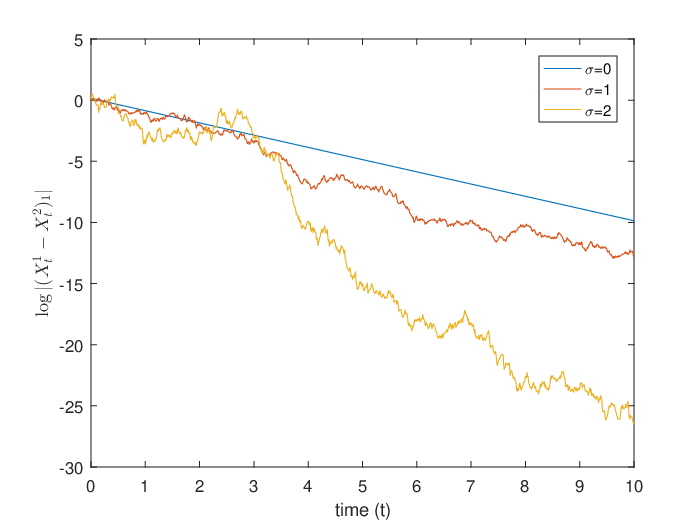
Note that for larger σ\sigma, the speed of consensus on average is faster. Note that these facts do not require the condition 2​λ>σ22\lambda>\sigma^{2} as can be seen in convergence analysis in Section 4. One can observe this result numerically. In Figures 2,3 and 4, we plot the positions of the particles for σ=0,1,2\sigma=0,1,2, respectively. Indeed, the particles seem to converge faster, as σ\sigma increases. In Figure 5, we plot a sample path of log⁡|xt1,1−xt2,1|\log|x_{t}^{1,1}-x_{t}^{2,1}| for σ=0,1,2\sigma=0,1,2. As expected, the graph for σ=0\sigma=0 is linear, and the function eventually decays faster for large σ\sigma.

Refer to caption
Figure 2. Temporal evolution of state configuration for t=0,1,2,10t=0,1,2,10 (σ=0)(\sigma=0).
Refer to caption
Figure 3. Temporal evolution of state configuration for t=0,1,2,10t=0,1,2,10 (σ=1)(\sigma=1).
Refer to caption
Figure 4. Temporal evolution of state configuration for t=0,1,2,10t=0,1,2,10 (σ=2)(\sigma=2).
Refer to caption
Figure 5. Graph of log⁡|xt1,1−xt2,1|\log|x_{t}^{1,1}-x_{t}^{2,1}| for σ=0,1,2\sigma=0,1,2.

5.2. Discrete algorithm

Recall the discrete algorithm:

(5.1) {Xn+1i=Xni+λ​h​∑k=1Nψnk​(Xnk−Xni)+σ​h​∑k=1N∑l=1dψnk​(xnk,l−xni,l)​Znl​el,ψkn:=e−β​L​(Xnk)∑i=1Ne−β​L​(Xni),1≤k≤N,n=0,1,⋯.\begin{cases}\displaystyle X^{i}_{n+1}=X^{i}_{n}+\lambda h\sum_{k=1}^{N}\psi_{n}^{k}(X_{n}^{k}-X_{n}^{i})+\sigma\sqrt{h}\sum_{k=1}^{N}\sum_{l=1}^{d}\psi_{n}^{k}(x_{n}^{k,l}-x_{n}^{i,l})Z^{l}_{n}e_{l},\\ \displaystyle\psi^{k}_{n}:=\frac{e^{-\beta L(X^{k}_{n})}}{\sum_{i=1}^{N}e^{-\beta L(X^{i}_{n})}},\quad 1\leq k\leq N,\quad n=0,1,\cdots.\end{cases}

In this subsection, we study the formation of global consensus for the discrete algorithm (5.1) numerically. In Theorem 3.4, we have shown that if m:=λ−σ22−λ2​h2>0m:=\lambda-\frac{\sigma^{2}}{2}-\frac{\lambda^{2}h}{2}>0 then the quantity Δni​j:=|Xni−Xnj|\Delta_{n}^{ij}:=|X_{n}^{i}-X_{n}^{j}| tends to zero almost surely, as n→∞n\to\infty with a decay rate approximately exp⁡(−12​m​n​h)\exp(-\frac{1}{2}mnh). Figure 6 indicates that this result is not optimal. To compute 𝔼⁡[log⁡|xt1,1−xt2,1|]\mathbb{E}\Big[\log|x_{t}^{1,1}-x_{t}^{2,1}|\Big], we simulated 100 sample paths and then took average of those paths. Although 2​λ<σ22\lambda<\sigma^{2} for σ=2\sigma=2, Δni​j\Delta_{n}^{ij} converges in this case. Moreover, although the decay rate obtained in Theorem 3.4 decreases, as σ\sigma increases, one can see that the decay rate increases as σ\sigma increases.

Refer to caption
Figure 6. Graph of 𝔼⁡[log⁡|xn1,1−xn2,1|]\mathbb{E}\Big[\log|x_{n}^{1,1}-x_{n}^{2,1}|\Big] for σ=0,1,2\sigma=0,1,2.

6. conclusion

In this paper, we have provided a rigorous convergence analysis for the first-order consensus-based optimization algorithm. In [5], the convergence was understood using the corresponding mean-field limit, the Fokker-Planck equation. Thus, the convergence of the original CBO algorithm remains unresolved there. The main contribution of this work is to provide the convergence analysis directly on the CBO algorithm model at the particle level. After rewriting the given continuous optimization algorithm into a first-order consensus form, we use the detailed structure of the coupling term to derive an exact formula for the state differences. Our explicit formula shows that global consensus will emerge for any initial data, whereas in order to prove the convergence toward a global minimum, we need a sufficient condition–which is dimension independent– for systems parameters and initial data to show that the global consensus state tends to a global minimum, as the reciprocal of temperature tends to infinity using Laplace’s principle. The emergence of global consensus will emerge for continuous and discrete algorithms. However, we can obtain the convergence analysis only for the continuous algorithm due to Ito’s stochastic analysis for twice differentiable and bounded objective functions. In contrast, for discrete algorithm, we do not have available mathematical tools to derive convergence analysis at present.

There are several issues which we cannot deal with in this paper. To name a few, it will be interesting to relax the regularity of the objective function to the less regular objective function, at least continuous one. Finally, random batch methods were used to reduce the computational cost of the NN-term summation in [5, 14] in which convergence remains as an open question.

Moreover, it will be interesting to see whether our presented analysis can be applied to other metaheuristic algorithms based on the swarm intelligence. These issues will be discussed in a future work.

References

  • [1] Acebron, J. A., Bonilla, L. L., Pérez Vicente, C. J. P., Ritort, F. and Spigler, R.: The Kuramoto model: A simple paradigm for synchronization phenomena. Rev. Mod. Phys. 77 (2005), 137-185.
  • [2] Ahn, S. M. and Ha, S.-Y.: Stochastic flocking dynamics of the Cucker-Smale model with multiplicative white noises. J. Math. Physics. 51 (2011), 103301.
  • [3] Albi, G., Bellomo, N., Fermo, L., Ha, S.-Y., Pareschi, L., Poyato, D. and Soler, J.: Vehicular traffic, crowds, and swarms. On the kinetic theory approach towards research perspectives. Math. Models Methods Appl. Sci. 29 (2019), 1901-2005.
  • [4] Bertsekas, D.: Convex Analysis and Optimization. Athena Scientific. 2003.
  • [5] Carrillo, J. A., Jin, S., Li, L. and Zhu, Y.: A consensus-based global optimization method for high dimensional machine learning problems. Submitted.
  • [6] Carrillo, J., Choi, Y.-P., Totzeck, C. and Tse, O.: An analytical framework for consensus-based global optimization method. Mathematical Models and Methods in Applied Sciences 28 (2018), 1037-1066.
  • [7] Choi, Y.-P., Ha, S.-Y. and Li, Z.: Emergent dynamics of the Cucker-Smale flocking model and its variants. In N. Bellomo, P. Degond, and E. Tadmor (Eds.), Active Particles Vol.I Theory, Models, Applications (tentative title), Series: Modeling and Simulation in Science and Technology, Birkhauser, Springer. 2017.
  • [8] Eberhart, R. and Kennedy, J.: Particle swarm optimization. Proceedings of the IEEE International Conference on Neural Networks 4 (1995), 1942-1948.
  • [9] Cucker, F. and Smale, S.: On the mathematics of emergence. Japanese Journal of Mathematics 2 (2007), 197-227.
  • [10] Fang, D., Ha, S.-Y. and Jin, S.: Emergent behaviors of the Cucker-Smale ensemble under attractive-repulsive couplings and Rayleigh frictions. Math. Models Methods Appl. Sci. 29 (2019), 1349-1385
  • [11] Ha, S.-Y. and Liu, J.-G.: A simple proof of Cucker-Smale flocking dynamics and mean-field limit. Commun. Math. Sci. 7 (2009), 297-325.
  • [12] Ha, S.-Y., Lee, K. and Levy, D.: Emergence of time-asymptotic flocking in a stochastic Cucker-Smale system. Commun. Math. Sci. 7 (2009), 453-469.
  • [13] Holland, J. H.: Genetic algorithms. Scientific American 267 (1992), 66-73.
  • [14] Jin, S. Li, L. and Liu, J.-G.: Random batch methods(RBM) for interacting particle systems. J. Comp. Phys., to appear. arXiv:1812.10575, 2018.
  • [15] Kennedy, J.: Swarm intelligence. Handbook of nature-inspired and innovative computing. Springer, 187-219 (2006).
  • [16] Kirkpatrick, S., Gelatt, C. D. and Vecchi, M. P.: Optimization by simulated annealing. Science 220 (1983), 671-680.
  • [17] Kolokolnikov, T., Carrillo, J. A., Bertozzi, A., Fetecau, R. and Lewis, M.: Emergent behavior in a multi-particle systems with non-local interactions. Physica D 260 (2013), 1-4.
  • [18] Kuramoto, Y.: Chemical oscillations, waves and turbulence. Springer-Verlag, Berlin, 1984.
  • [19] Kuramoto, Y.: International symposium on mathematical problems in mathematical physics. Lecture Notes Theor. Phys. 30 (1975), 420.
  • [20] Laarhoven, P. J. M. van and Aarts, E. H. L.: Simulated annealing: theory and applications. D. Reidel Publishing Co., Dordrecht, 1987.
  • [21] Motsch, S. and Tadmor, E.: Heterophilious dynamics enhances consensus. SIAM. Rev. 56 (2014), 577-621.
  • [22] Peskin, C. S.: Mathematical aspects of heart physiology. Courant Institute of Mathematical Sciences, New York, 1975.
  • [23] Pinnau, R., Totzeck, C., Tse, O. and Martin, S.: A consensus-based model for global optimization and its mean-field limit. Math. Models Methods Appl. Sci. 27 (2017), 183-204.
  • [24] Pikovsky, A., Rosenblum, M. and Kurths, J.: Synchronization: A universal concept in nonlinear sciences. Cambridge University Press, Cambridge, 2001.
  • [25] Totzeck, C. Pinnau, R., Blauth, S. and Schotthófer, S.: A numerical comparison of consensus-based global optimization to other particle-based global optimization scheme. Proceedings in Applied Mathematics and Mechanics, 18, 2018.
  • [26] Vicsek, T. and Zefeiris, A.: Collective motion. Phys. Rep. 517 (2012), 71-140.
  • [27] Yang, X.-S.: Nature-inspired metaheuristic algorithms. Luniver Press, 2010.
  • [28] Yang, X.-S., Deb, S., Zhao, Y.-X., Fong, S. and He, X.: Swarm intelligence: past, present and future. Soft Comput 22 (2018), 5923-5933.