On the Packing of Stiff Rods on Ellipsoids Part I - Geometry

Packing of filaments inside volumes of a given shape is an important problem in many fields. From packing of genetic material inside viral capsidsMarenduzzo et al. 2010; Katzav et al. 2006; Boué and Katzav 2007; Purohit et al. 2003; Angelescu and Linse 2008, through ordering of micro-tubules near plant cell wallsUyttewaal et al. 2012; Burk and Ye 2002; Stoop 2011, to spooling of filaments in industrial application Vetter et al. 2013; Vetter 2015; Pineirua et al. 2013 and other biopolymers such as spider silk Elettro 2015; Elettro et al. 2017a; Elettro et al. 2017b; Elsner et al. 2012. These type of problems are hard as they typically involve a compromise between elastic energy and entropic constraints. As a result, most approaches to these problems involve highly symmetric volumes and are mostly numerical. This paper’s aim is to gain further analytical understanding of systems which are not highly symmetric, using differential geometry, study of entropic efects and self avoidance is largely postponed to a later paper. As concrete examples, we consider plant cells where shape regulation is important and microtubules play a significant role and the packing of genetic material inside viral capsids. While these two examples seem very different, both are essentially problems of packing long semi-flexible filaments. Additionally, the authors hope that this work will serve as an inspiration for applying similar methods from differential geometry to study other systems, and not only the packing of filaments on surfaces.

In the context of plant tissue, the confinement of microtubules (MT) in the cell membrane, and especially, the possible transition from disordered to partially ordered packing is thought to be the origin of important morphogenetic and growth regulating mechanisms. The location of leaves on the stem, anisotropic cell expansion, as in roots and stems, and the evolution of anisotropic mechanical properties of extended leaf tissue are few examples in which mechanical and geometrical asymmetries appear. In plant cells, cellulose fibrils in the cell wall are the carrier of mechanical load. Orientation of cortical MT dictates the orientation of cellulose fibrils deposition in the cell wall Burk and Ye 2002. Therefore, anisotropic MT orientation would lead to anisotropic cellulose deposition, and, thus, to anisotropic mechanical properties of the cell. This, in turn, would lead to its anisotropic growth and to shape evolution of the tissue. But what sets MT orientation at the single cell level? The suggestion that mechanical stress directly affects MT orientation, was supported by pointing to the correlations between MT orientation and the directions of principal stresses in evolving meristems Uyttewaal et al. 2012.On the other hand, it is not clear how stress or strain in the cell wall can affect the cell membrane Fisher and Cyr 1998; Somerville et al. 2004. In addition, the effect of applied stress on mechanical properties of a leaf appeared only after a delay of several hours Sahaf and Sharon 2016. This suggests that an integral mechanism, which is common in other growth regulation mechanisms Oh et al. 2014; Chaiwanon et al. 2016, could be in action. Alternative approaches, suggest that the cell shape, and particularly, its anisotropy is a dominant factor in MT ordering. The two approaches are, in fact, closely related: Considering a circular cell, an integral over the strain determines the cell’s anisotropy. We therefore pose the questions of what are the leading effects of cell shape on the disordered-aligned transition of MT.

In the context of viral capsids there is ultimate necessity for the genetic material to be orderly packed inside the capsid in order to assure effective infection. This is so important because once the genetic material is packed inside the capsid it has no active sources of energy to support its injection, except for the elastic energy stored in the structure. It has been convincingly argued Marenduzzo et al. 2010; Katzav et al. 2006; Purohit et al. 2003 that the size of the capsid plays an important role in piloting towards an ordered structure based on both entropic and energetic considerations, showing that active biological control over ordering the spool could be seriously reduced. In particular, a continuous phase transition between a disordered phase (for large capsids) and an ordered phase (for small capsids) has been found. The spontaneous formation of virus capsids from multiple copies of capsid proteins is itself a fascinating example of supramolecular self-assembling processes Fejer 2020. Most known viruses protect their genome with icosahedral capsids, which is often modelled as a spherical cavity. However, other capsid morphologies exist as well, notably elongated, often ellipsoid, structures. The bacteriophage $\phi 29$ has elongated capsids with size of about $42{\rm nm}\times 54{\rm nm}$ leading to an aspect ratio of $4:5$ Marenduzzo 2009; Ali et al. 2006. The capsid of archaeal virus Sulfolobus ellipsoid virus 1 (SEV1) Wang et al. 2018 is that of a prolate ellipsoid with principal axes of $78{\rm nm}\times 115{\rm nm}$ hence aspect ratio of about $2:3$. Other important examples include the human virus, HIV-1, where experiments have demonstrated the self-assembly of viral capsid proteins into elongated shapes both in vitro and in vivo Krishna et al. 2010 with varying aspect ratios depending on the precise conditions during the assembly process, notably the interaction between the building block proteins. An interesting example is the case of extremely elongated capsids in mutant T4 phages Rao and Leffers 1993 with aspect ratios in the range $1:2$-$1:3$ leading to a twisted toroidal configuration of DNA inside them. An immediate question that comes to mind is: does the shape of the capsid affect the ordering phase transition of the genetic material in the capsid compared to the spherical case? Simulations performed by different groups Marenduzzo et al. 2010; Vetter et al. 2013; Marenduzzo 2008; Marenduzzo 2009 indicate that packings in oblate spheroids and scalene ellipsoids are energetically preferred to spheres. In simple words, it seems that the elongated container tends to order the structure more than a spherical one. Furthermore, it was observed in simulations Marenduzzo 2009; Ali et al. 2006; Petrov et al. 2007; Petrov and Harvey 2008; Petrov et al. 2009 that the kind of order of the genetic material changes, and attains a nematically ordered structure with twist (also called twisted toroidal conformations Petrov et al. 2007), as opposed to a spool-like one in spherical capsids. The different simulations are not clear about the source of this effect. Some suggest that the toroidal packing arranges itself along the longest possible dimension to minimize the bending stress (and hence the elastic energy) Petrov et al. 2007, while others put more emphasis on entropic effect Jun and Mulder 2006. In this paper we want to clarify the energetic aspects of packing an elastic rod, and in particular the enhanced ordering emanating from the elongated geometry, while in a future publication we will focus on entropic effects.

We begin by assuming a a phantom ,i.e. non - self - avoiding, unstretchable, filament of thickness $t$ whose midline is given by ${\bf R}(s)=\left\{X(s),Y(s),Z(s)\right\}$ where $s$ is the arclength along the rod. The bending energy of such a rod is

$\displaystyle E$

$\displaystyle=\frac{{\varepsilon}t^{4}}{2}\int\left|\ddot{\bf R}(s)\right|^{2}\,\text{d}s=\frac{{\varepsilon}t^{4}}{2}\int\left(\ddot{X}^{2}+\ddot{Y}^{2}+\ddot{Z}^{2}\right)\,\text{d}s$

(1)

where $\ddot{Q}=\partial_{s}^{2}{Q}$ is the second derivative of the quantity $Q(s)$, and ${\varepsilon}$ is the rod’s Young’s modulus. At zero temperature, the rod’s configuration is the global minimizer of Eq.(1), subjected to the constraint of lying on the surface of an ellipsoid - $X^{2}(s)+Y^{2}(s)+Z^{2}(s)/(1+\delta)^{2}=1$, where $\delta>-1$ is called the flattening of the ellipsoid, and is related to the usual definition of eccentricity $e$, via $e^{2}=\delta(2+\delta)$ Newton 1726; Bessel et al. 2009a; Bessel et al. 2009b. A vanishing flattening, $\delta=0$, corresponds to a sphere. Negative values of $\delta$ in the range $-1<\delta<0$ describe an oblate spheroid, while positive values, $\delta>0$ is a prolate spheroid. The problem of finding the global energy minimizer is difficult, as the system is clearly highly frustrated. We therefore use a geometrical approach, and describe the rod using its curvatures rather than the configuration $\mathbf{R}$. We start by assigning a generalized Frenet - Serret frame (see Panyukov and Rabin 2000; Grossman et al. 2016; Grossman et al. 2018), $\left\{\mathbf{t}_{1},\mathbf{t}_{2},\mathbf{t}_{3}\right\}$, being the tangent, bi-normal and normal vectors of the rod, respectively, as follows. Given $\mathbf{f}=\left\{X(x,y),Y(x,y),Z(x,y)\right\}$, the surface configuration ($x,y$ being coordinates on the surface), and $\mathbf{\hat{n}}$ the normal to the surface, we choose a local orthonormal in-plane frame along the rod, using a Darboux frame on the surface $\left\{\partial_{x}\mathbf{f},\partial_{y}\mathbf{f},\mathbf{\hat{n}}\right\}$ we define the Frenet - Serret frame, $\left\{\mathbf{t}_{1},\mathbf{t}_{2},\mathbf{t}_{3}\right\}$, and the in - plane surface tangent and normal vectors $e_{1}^{\mu}$ and $e_{2}^{\mu}$:

	$\displaystyle\mathbf{t}_{1}$	$\displaystyle=\dot{\bf R}=e_{1}^{\mu}\partial_{\mu}\mathbf{f}$		(2a)
	$\displaystyle\mathbf{t}_{2}$	$\displaystyle=e_{2}^{\mu}\partial_{\mu}\mathbf{f}$		(2b)
	$\displaystyle\mathbf{t}_{3}$	$\displaystyle=\mathbf{\hat{n}}.$		(2c)
Orthonormality dictates, that the inner products satisfy $e_{1}^{\mu}e_{1\mu}=a_{\mu\nu}e_{1}^{\mu}e_{1}^{\nu}=1=e_{2}^{\mu}e_{2\mu}$, and $e_{1}^{\mu}e_{2\mu}=0$, where $a_{\mu\nu}=\partial_{\mu}\mathbf{f}\cdot\partial_{\nu}\mathbf{f}$ is the induced metric on the surface, and $\mu,\nu\in\left\{x,y\right\}$.

It is then straightforward to show that $\mathbf{t}_{\alpha}$, $\alpha\in\{1,2\}$ satisfy the equations,

$\displaystyle\dot{\mathbf{t}}_{\alpha}$

$\displaystyle=\partial_{s}\mathbf{t}_{\alpha}=(\partial_{s}e_{\alpha}^{\mu})\partial_{\mu}\mathbf{f}+e_{1}^{\mu}e_{\alpha}^{\nu}\partial_{\mu}\partial_{\nu}\mathbf{f}=-\kappa_{g}\sum_{\beta}\epsilon_{\alpha\beta}e_{\beta}^{\mu}\partial_{\mu}\mathbf{f}+e_{1}^{\mu}e_{\alpha}^{\nu}b_{\mu\nu}\mathbf{t}_{3},$

(3)

and $\mathbf{t}_{3}$ satisfies

$\displaystyle\dot{\mathbf{t}}_{3}=-\sum_{\alpha}e_{1}^{\mu}e_{\alpha}^{\nu}b_{\mu\nu}\mathbf{t}_{\alpha}.$

(4)

Here $b_{\mu\nu}=\partial_{\mu}\partial_{\nu}\mathbf{f}\cdot\hat{\mathbf{n}}$ is the second fundamental form of the confining surface, $\kappa_{g}$ is the geodesic curvature of the rod on the surface, and $\epsilon_{\alpha\beta}$ is the $2\times 2$ antisymmetric (Levi-Civita) symbol. Deriving Eq. (3), we used the fact that for a general curve, namely a non geodesic one, on the surface $e_{1}^{\mu}$ and $e_{2}^{\mu}$ are transported via the equation

$\displaystyle\nabla_{s}e_{\alpha}^{\mu}$

$\displaystyle=\partial_{s}e_{\alpha}^{\mu}+e_{1}^{\rho}e_{\alpha}^{\sigma}\Gamma_{\rho\sigma}^{\mu}=-\kappa_{g}\sum_{\beta}\epsilon_{\alpha\beta}\,e_{\beta}^{\mu}$

(5)

where $\nabla_{s}$ is the covariant derivative along the curve, and the Christoffel symbols, given a configuration

$\displaystyle a_{\rho\lambda}\Gamma_{\mu\nu}^{\lambda}=\partial_{\mu}\partial_{\nu}\mathbf{f}\cdot\partial_{\rho}\mathbf{f}.$

(6)

Eqs. (3) and (4) can be rewritten in matrix form as

$\displaystyle\left(\begin{array}[]{c}\dot{\mathbf{t}}_{1}(s)\\ \dot{\mathbf{t}}_{2}(s)\\ \dot{\mathbf{t}}_{3}(s)\end{array}\right)=-\left(\begin{array}[]{c c c}0&\kappa_{g}&-l\\ -\kappa_{g}&0&m\\ l&-m&0\end{array}\right)\left(\begin{array}[]{c}\mathbf{t}_{1}(s)\\ \mathbf{t}_{2}(s)\\ \mathbf{t}_{3}(s)\end{array}\right)$

where we defined the curvatures

	$\displaystyle l$	$\displaystyle=e_{1}^{\mu}e_{1}^{\nu}b_{\mu\nu}$		(16a)
	$\displaystyle m$	$\displaystyle=-e_{1}^{\mu}e_{2}^{\nu}b_{\mu\nu}$		(16b)

The formal solution of Eq. (On the Packing of Stiff Rods on Ellipsoids Part I - Geometry) is

$\displaystyle\left(\begin{array}[]{c}\mathbf{t}_{1}(s)\\ \mathbf{t}_{2}(s)\\ \mathbf{t}_{3}(s)\end{array}\right)=T_{s}\left[\exp\left(-\int\limits_{0}^{s}\,\text{d}s^{\prime}\left(\begin{array}[]{c c c}0&\kappa_{g}&-l\\ -\kappa_{g}&0&m\\ l&-m&0\end{array}\right)\right)\right]\left(\begin{array}[]{c}\mathbf{t}_{1}(0)\\ \mathbf{t}_{2}(0)\\ \mathbf{t}_{3}(0)\end{array}\right)$

where we use the definition of the position ordering operator $T_{s}$

$\displaystyle T_{s}\exp\left[{\int\limits_{0}^{s}M\,\text{d}s^{\prime}}\right]=\lim\limits_{k\rightarrow\infty}e^{M(s_{0})\Delta s}e^{M(s_{1})\Delta s}\dots e^{M(s_{k})\Delta s},$

(26)

where $\Delta s=\frac{s}{k}$, and $s_{k}=k\Delta s$. The rod configuration is then given by

$\displaystyle\mathbf{R}(s)=\mathbf{R}(0)+\int\limits_{0}^{s}\mathbf{t}_{1}(s^{\prime})\,\text{d}s^{\prime}$

(27)

The elastic energy (1) assumes the form

$\displaystyle E$

$\displaystyle=\frac{\varepsilon t^{4}}{2}\int\,\text{d}s\left(\kappa_{g}^{2}+l^{2}\right).$

(28)

While this seems to be a simpler functional than the one given in Eq. (1), one must remember that $l$ itself is a functional of the geodesic curvature, $\kappa_{g}(s)$ (via Eq. (5)). Since we are searching for global minimizers (for infinitely long rods) we seek to minimize the total energy per unit length.

$\displaystyle\bar{E}$

$\displaystyle=\frac{E}{L}=E_{0}\frac{\displaystyle\int\left(\kappa_{g}^{2}+l^{2}\right)\,\text{d}s}{\displaystyle\int\,\text{d}s},$

(29)

where we define the energy scale $E_{0}=\frac{\varepsilon t^{4}}{2}$.

Eq. (29) reveals an important property of the energy minimizing problem: while the normal curvature, $l$, is a property of the surface, the geodesic curvature, $k_{g}$, can be eliminated by a proper selection of the rod configuration. These configurations are geodesics, which locally minimize Eq. (29). As shown later (appendix A), for any positive flattening, $\delta>0$, no geodesic is a global minimizer. However, the true global minimizer cannot deviate significantly from a geodesic (see appendix B). Therefore, we conclude geodesics are good approximations,an limit ourselves to their study, which significantly simplifies the problem.

We begin by parametrising the surface of the ellipsoid using $\theta$ (polar) and $\phi$ (azimuthal) angles, and subsequently finding the geodesics in terms of these coordinates:

	$\displaystyle X$	$\displaystyle=\cos\phi\sin\theta$
	$\displaystyle Y$	$\displaystyle=\sin\phi\sin\theta$		(30)
	$\displaystyle Z$	$\displaystyle=(1+\delta)\cos\theta$

The metric $\mathbf{a}$, the second fundamental form $\mathbf{b}$ and the shape operator (extrinsic curvature) $\mathbf{S}$ Do Carmo 2016 of the surface are then given by

	$\displaystyle\mathbf{a}$	$\displaystyle=\left(\begin{array}[]{cc}1+\delta(2+\delta)\sin^{2}\theta&0\\ 0&\sin^{2}\theta\end{array}\right)$
	$\displaystyle\mathbf{b}$	$\displaystyle=-\frac{1+\delta}{\sqrt{1+\delta(2+\delta)\sin^{2}\theta}}\left(\begin{array}[]{cc}1&0\\ 0&\sin^{2}\theta\end{array}\right)$
	$\displaystyle\mathbf{S}$	$\displaystyle=\mathbf{a}^{-1}\mathbf{b}=-\left(\begin{array}[]{cc}\frac{1+\delta}{({1+\delta(2+\delta)\sin^{2}\theta})^{3/2}}&0\\ 0&\frac{1+\delta}{\sqrt{1+\delta(2+\delta)\sin^{2}\theta}}\end{array}\right).$

Since the metric is independent of $\phi$, there is a conserved, conjugate “angular momentum” $\omega$, which is related to the “angular velocity” $\dot{\phi}$ , and is the generator of rotations around the symmetry axis of the ellipsoid found by solving the geodesic equation for $\phi$ coordinate Do Carmo 2016:

	$\displaystyle\frac{d}{ds}\left(a_{\phi\mu}\frac{dx^{\mu}}{ds}\right)$	$\displaystyle=0$		(37)
Since the metric is diagonal, only $a_{\phi\phi}=\sin^{2}\theta$ contributes to the sum -
	$\displaystyle\frac{d}{ds}\left(a_{\phi\phi}\frac{d\phi}{ds}\right)$	$\displaystyle=0$		(38)
in other words, this is a constant, which we mark by $\omega$
	$\displaystyle\sin^{2}\theta\frac{d\phi^{\mu}}{ds}$	$\displaystyle=\omega=const.$		(39)

Thus

$\displaystyle\dot{\phi}(s)$

$\displaystyle=\frac{\omega}{\sin^{2}\theta},$

(40)

where arc-length normalization of $s$ requires $-1\leq\omega\leq 1$. Instead of solving the geodesic equation for $\theta$ we may impose normalization, $e^{\mu}_{1}e_{1}^{\nu}a_{\mu\nu}=1$ and get the equation

$\displaystyle\left(1+2\delta\sin^{2}\theta+\delta^{2}\sin^{2}\theta\right)\dot{\theta}^{2}$

$\displaystyle=1-\frac{\omega^{2}}{\sin^{2}\theta}.$

(41)

By taking $\sin^{2}\theta$ as a common factor we get

$\displaystyle\left(\frac{1}{\sin^{2}\theta}+2\delta+\delta^{2}\right)\sin^{2}\theta\dot{\theta}^{2}$

$\displaystyle=1-\frac{\omega^{2}}{\sin^{2}\theta}$

(42)

leading to

$\displaystyle\left(\frac{d}{ds}\cos\theta\right)^{2}$

$\displaystyle=\frac{1-\frac{\omega^{2}}{\sin^{2}\theta}}{\left(\frac{1}{\sin^{2}\theta}+2\delta+\delta^{2}\right)}.$

(43)

Rewriting everything in terms of $\cos\theta$ we get the equation

$\displaystyle\left(\frac{d}{ds}\cos\theta\right)^{2}$

$\displaystyle=\frac{1-\omega^{2}-\cos^{2}\theta}{\left[(1+\delta)^{2}-2\delta\cos^{2}\theta-\delta^{2}\cos^{2}\theta\right]}.$

(44)

Which after defining $x(s)=\cos\left[\theta(s)\right]$, and marking $\dot{x}=\frac{dx}{ds}$ turns into

$\displaystyle(\dot{x})^{2}$

$\displaystyle=\frac{1-\omega^{2}-x^{2}}{(1+\delta)^{2}-(2\delta+\delta^{2})x^{2}}.$

(45)

Separating variables and integrating we obtain

$\displaystyle\int\frac{\sqrt{(1+\delta)^{2}-(2\delta+\delta^{2})x^{2}}\,\text{d}x}{\sqrt{1-\omega^{2}-x^{2}}}$

$\displaystyle=\pm\int\,\text{d}s+s_{0}.$

(46)

This equation is integrable, giving rise to

$\displaystyle(1+\delta)\mathcal{E}\left[\sin^{-1}\left(\frac{x}{\sqrt{1-\omega^{2}}}\right)\Bigg|\frac{\delta(\delta+2)\left(1-\omega^{2}\right)}{(\delta+1)^{2}}\right]$

$\displaystyle=\pm s+s_{0}$

(47)

where $\mathcal{E}[\theta|m]=\int\limits_{0}^{\theta}\sqrt{1-m\sin^{2}\phi}\,\text{d}\phi$ is the incomplete elliptic integral of the second kind Olver et al. 2010, and $s_{0}$ is determined by initial conditions. To find geodesics we now need to integrate Eq. (40), which can be done numerically. However, by virtue of rotational symmetry about the polar axis of the ellipsoid ($a_{\mu\nu}$ is independent of $\phi$, geodesics are parametrized by $\omega$ alone), we can disregard exact solutions of $\phi(s)$ when looking for minimizing geodesics, and we can immediately look for a minimizer of Eq. (29) (see Eq. (49)).

Evaluating $\bar{E}$ on geodesics, we find that by virtue Eq. (47), instead of integrating over $s$ we may integrate over $\theta$ (or rather over $x$) where we find

$\displaystyle\frac{\,\text{d}s}{\,\text{d}x}=\sqrt{\frac{(1+\delta)^{2}-\delta(2+\delta)x^{2}}{1-\omega^{2}-x^{2}}}.$

(48)

Thus, focusing on geodesics we look to minimize the following energy functional:

	$\displaystyle\frac{\bar{E}(\omega,\delta)}{E_{0}}$	$\displaystyle=\frac{\displaystyle\int E\,\text{d}s}{\displaystyle\int\,\text{d}s}=\frac{\displaystyle\int_{-\sqrt{1-\omega^{2}}}^{\sqrt{1-\omega^{2}}}\frac{\left(1+\delta\right)^{2}\left[1+\delta(2+\delta)\omega^{2}\right]^{2}}{\left[1+\delta(\delta+2)\left(1-x^{2}\right)\right]^{3}}\sqrt{\frac{1+(1-x^{2})\delta(2+\delta)}{1-x^{2}-\omega^{2}}}\,\text{d}x}{\displaystyle\int_{-\sqrt{1-\omega^{2}}}^{\sqrt{1-\omega^{2}}}\sqrt{\frac{1+(1-x^{2})\delta(2+\delta)}{1-x^{2}-\omega^{2}}}\,\text{d}x}$		(49)
		$\displaystyle=\frac{2\left[2+\delta(2+\delta)(1+\omega^{2})\right]\mathcal{E}\left[\frac{\delta(2+\delta)(1-\omega^{2})}{(1+\delta)^{2}}\right]-2\left[1+\delta(2+\delta)\omega^{2}\right]\mathcal{K}\left[\frac{\delta(2+\delta)(1-\omega^{2})}{(1+\delta)^{2}}\right]}{3(1+\delta)^{2}\mathcal{E}\left[\frac{\delta(2+\delta)(1-\omega^{2})}{(1+\delta)^{2}}\right]}$		(50)
		$\displaystyle=\frac{2\left[2+\delta(2+\delta)(1+\omega^{2})\right]}{6(1+\delta)^{2}}-\frac{2\left[1+\delta(2+\delta)\omega^{2}\right]\mathcal{K}\left[\frac{\delta(2+\delta)(1-\omega^{2})}{(1+\delta)^{2}}\right]}{3(1+\delta)^{2}\mathcal{E}\left[\frac{\delta(2+\delta)(1-\omega^{2})}{(1+\delta)^{2}}\right]}$		(51)

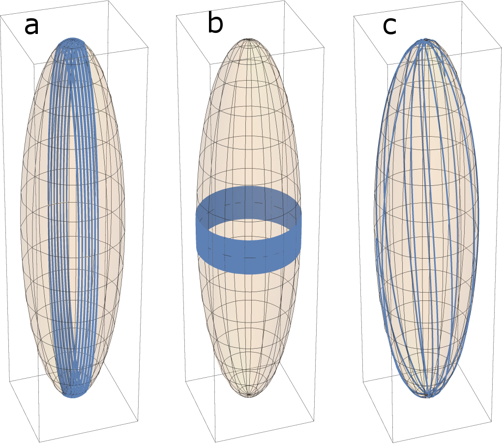
where $\mathcal{E}[m]=\int_{0}^{\pi/2}\sqrt{1-m\sin^{2}\theta}\,\text{d}\theta$ and $\mathcal{K}[m]=\int_{0}^{\pi/2}\left({\sqrt{1-m\sin^{2}\theta}}\right)^{-1}\,\text{d}\theta$ are the complete elliptic integrals of the second and first kind Olver et al. 2010, respectively. Plotting $\bar{E}$ for different values of $\delta$ as a function of $\omega$ (see Fig.1), it is easily seen that for $\delta<0$ only $\omega=\pm 1$ are the minima, this is true for every $-1<\delta<0$ and ,as seen in appendix A, these solution are stable. We therefore conclude that equatorial geodesics are the global minimizers for oblate spheroids (see Fig. 2(a)). Not surprisingly, in the case of a sphere ($\delta=0$) we find that any geodesic is a global minimizer. These results (for $\delta\leq 0$) are indeed very intuitive. In contrast, a more complex behaviour arises in the case of prolate spheroids ($\delta>0$), where we observe a sharp transition at a critical flattening $\delta^{*}$ (Fig. 1, see Fig. 2(b) and (c) for visualization of possible curves).

We mark by $\omega_{m}(\delta)$ the minimizer of $\bar{E}(\omega,\delta)$, and it’s energy by $\bar{E}(\omega_{m}(\delta))=\bar{E}(\omega_{m}(\delta),\delta)$ i.e. the globally minimizing geodesic, as a function of the flattening, $\delta$, and plot it (Fig. 3). We find that for $0<\delta\leq\delta^{*}$ polar geodesics ($\omega_{m}=0$) are the minimizers of $\bar{E}$, while for $\delta>\delta^{*}$, $\omega_{m}(\delta)\neq 0$. Solving numerically the requirement that the extremum at $\omega=0$ becomes a saddle $\left.\frac{\partial^{2}\bar{E}}{\partial\omega^{2}}\right|_{\omega=0}=0$, where

$\displaystyle\left.\frac{\partial^{2}\bar{E}}{\partial\omega^{2}}\right|_{\omega=0}=\frac{E_{0}}{3}\left[5-\frac{4}{(1+\delta)^{2}}+\frac{\mathcal{K}\left[\frac{\delta(2+\delta)}{(1+\delta)^{2}}\right]}{\mathcal{E}\left[\frac{\delta(2+\delta)}{(1+\delta)^{2}}\right]}\left(\frac{1}{(1+\delta)^{2}}\frac{\mathcal{K}\left[\frac{\delta(2+\delta)}{(1+\delta)^{2}}\right]}{\mathcal{E}\left[\frac{\delta(2+\delta)}{(1+\delta)^{2}}\right]}-2\right)\right],$

(52)

we find that $\delta^{*}\simeq 2.917$. It can now be shown that near the transition, as $\delta\rightarrow\delta^{*+}$, $\omega_{m}(\delta)\sim\sqrt{\delta-\delta^{*}}$.

In the limit of an infinitely eccentric ellipsoid we get

$\displaystyle\frac{\bar{E}}{E_{0}}\xrightarrow[\delta\rightarrow\infty]{}\frac{2}{3}+\frac{\omega^{2}}{3}\left(2-\frac{\mathcal{K}\left[1-\omega^{2}\right]}{\mathcal{E}\left[1-\omega^{2}\right]}\right),$

(53)

whose minimizer is $\omega\simeq\pm 0.255...$ This value corresponds to geodesics that intersect the equator at an angle of $\psi\simeq 75.22^{\circ}$ relative to the equator.

Why does this transition happen? Simply put, it is because for large $\delta$’s, the curvature at the poles becomes very large and dominant. Thus, the minimizing geodesic is such that it does not pass through the poles on one hand, yet it is still mainly directed towards the poles, as to gain as much as possible from the large difference in principal curvatures values. This result raises the question whether there is a non-geodesic solution that has a lower mean energy even for small $\delta$, one that does not pass through the poles. Indeed, as seen in appendix B, there must be such a solution, yet this solution is still close to a geodesic, and in any case the solution to the real physical problem must also take into account temperature, activity and self-avoidance. Our analysis sheds light on some aspects of the mechanisms governing the actual shape and suggests that a proper treatment should take into account the surface’s shape effect on the final configuration, as it serves as an ”external field” biasing the rod to align along the symmetries of the problem.

Finally, for $\delta\neq 0$, these solutions given above, which all have a preferred direction (i.e. they are not isotropic), are clearly preferable to any other curve that covers the ellipsoid isotropically. Any isotropic solution, that covers the ellipsoid, must have geodesic curvature, but for infinitely long filaments, one may create such a curve by slowly changing $\omega$ along a curve. In this ”quasi-static” limit we change $\omega$ without introducing any geodesic curvature. Such a curve gives a lower bound on the energy of isotropic curves and is given by averaging $\bar{E}$ over all $\omega$

$\displaystyle\bar{E}_{iso}(\delta)=\frac{\displaystyle\int\bar{E}(\omega,\delta)\,\text{d}\omega}{\displaystyle\int\bar{E}(\omega)\,\text{d}\omega}.$

(54)

From Fig. 4 it is clearly seen that a directional (non isotropic) configuration is preferable compared to an isotropic configuration, since the dashed blue line corresponding to $\bar{E}_{iso}(\delta)$ is higher than the red solid line describing the energy of the globally minimizing geodesics $\bar{E}\left(\omega_{m}(\delta)\right)$.

Before we conclude, a few words on the possible effect of self avoidance. Naturally, a full mechanical treatment of self avoiding filaments is hard. However we may still have a few insights using our geometrical approach. We have shown that as the ellipsoid elongates, and due to the growing curvature at the poles, a transition occurs, so that the minimizing configuration is no longer a polar geodesic. In the presence of self avoidance, this transition is likely to occur later, at higher values of $\delta$, depending on the strength of the self-avoiding interaction. The reason is that a polar geodesic - like path (see Fig. 5 a) allows (especially for thin filaments) a non-intersecting packing, in contrast to the solution for $\delta>\delta^{*}$. The energy associated with a self avoiding (SA) packing is (see appendix C)

	$\displaystyle\frac{\bar{E}_{SA}(c,\delta)}{E_{0}}$	$\displaystyle=\frac{2\arcsin(c)}{c\sqrt{1-c^{2}}+\arcsin(c)}\times\left(\frac{2\left(2+\delta(2+\delta)\right)}{3\left(1+\delta\right)^{2}}-\frac{\mathcal{K}\left[\frac{\delta(2+\delta)}{(1+\delta)^{2}}\right]}{3(1+\delta)^{2}\mathcal{E}\left[\frac{\delta(2+\delta)}{(1+\delta)^{2}}\right]}\right)$		(55)
		$\displaystyle=\frac{2\arcsin(c)}{c\sqrt{1-c^{2}}+\arcsin(c)}\times\bar{E}(\omega=0,\delta)$

where $1\geq c=\frac{tL}{A}=\frac{tL}{2\pi}\frac{\sqrt{\delta\left(2+\delta\right)}}{\sqrt{\delta\left(2+\delta\right)}+\left(1+\delta\right)^{2}\text{sec}^{-1}\left(1+\delta\right)}$ is the average surface density of the filament, and $t$ is the thickness of te filament. Nevertheless, when the flattening , $\delta$, is large enough, it is clear that even a self-avoiding system will prefer to minimize the bending energy by avoiding the poles. Since any self - intersecting configuration, must do so many times, proportionate to the filament density $c$, and by denoting the self - interaction energy per unit length in $u$ , we can express the energy of a self - crossing filament as $\bar{E}+uc$ ($u>0$ for self - avoidance). Thus, the condition of a self - interacting filament to change configuration from polar to a non-polar one is

$\displaystyle\bar{E}_{SA}(c,{\delta})\gtrsim\bar{E}\left({\omega_{m}}({\delta})\right)+uc,$

(56)

as this expression means that the energy of a non - intersecting, self - avoiding curve is larger than that of a self interacting curve, including the self- interaction term. At small $c$’s, $\bar{E}_{SA}(c,\delta)\simeq\bar{E}(\omega=0,\delta)\left(1+\frac{c^{2}}{3}\right)$. Expanding $\delta^{*}=\delta^{*}_{0}+\delta^{*}_{1}c$, where $\delta^{*}_{0}=2.917$ is the critical $\delta$ found earlier, and requiring equality in Eq. (56), using Eq. (55) gives us the dependence of $\delta^{*}$ on $c$

$\displaystyle\bar{E}(0,\delta^{*}_{0}+c\delta^{*}_{1})\left(1+\frac{c^{2}}{3}\right)$

$\displaystyle=\bar{E}\left({\omega_{m}}(\delta^{*}_{0}+c\delta^{*}_{1})\right)+uc,$

(57)

Expanding in orders of $c$ and keeping only leading orders, the above equation reduces to

$\displaystyle c\delta^{*}_{1}\left.\frac{\partial\bar{E}(0,\delta)}{\partial\delta}\right|_{\delta\rightarrow{\delta^{*}_{0}}^{+}}$

$\displaystyle=uc+c\delta^{*}_{1}\left.\frac{\partial\bar{E}\left({\omega_{m}}(\delta)\right)}{\partial\delta}\right|_{\delta\rightarrow{\delta^{*}_{0}}^{+}}.$

(58)

This can then be solved for $\delta^{*}_{1}$

$\displaystyle\delta^{*}_{1}$

$\displaystyle=\left.\frac{u}{\frac{\partial\bar{E}(0,\delta)}{\partial\delta}-\frac{\partial\bar{E}\left({\omega_{m}}(\delta)\right)}{\partial\delta}}\right|_{\delta\rightarrow{\delta^{*}_{0}}^{+}}.$

(59)

Since $\frac{\partial\bar{E}(0,\delta)}{\partial\delta}|_{\delta\rightarrow{\delta^{*}_{0}}^{+}}\geq 0$ and $\frac{\partial\bar{E}\left({\omega_{m}}(\delta)\right)}{\partial\delta}|_{\delta\rightarrow{\delta^{*}_{0}}^{+}}<0$, it is clear that $\delta^{*}_{1}>0$ therefore self avoidance indeed postpones the aforementioned transition.

Another possible effect of self avoidance is the appearance of meta-stable states, where the filament packs without crossing, such as paths with $\omega\sim 1$ that wrap many times around the ellipsoid (see Fig. 5 b), but any deviation from this configuration means that the filament must cross itself many times (Fig. 5 c). At high densities and strong self avoiding interactions , such a configuration is likely to be meta-stable.

To conclude, we have used a geometrical approach to show that the shape of an ellipsoid acts as an ”external field” that orders the orientation of a stiff filaments on it’s surface. We have shown that energy, not only entropy, plays a significant role in ordering the packing of filaments inside non-spherical volumes. By the use of geodesics to allow for a simple analytical treatment, we have directly shown that in general, filaments will tend to align with the long dimension of the ellipsoid. However, this is not completely accurate, since (at least for geodesics) the transition is likely to occur in very long ellipsoids, where the globally bending minimizing curve no longer passes through the poles. The transition is somewhat sensitive to the geometry,e.g. within a model of cylinder with spherical caps, no such transition will occur as a function of elongation as the curvature does not depend on the the flattening in such a case. Nevertheless, these results reflect similar numerical result as in Mirabet et al. 2018; Vetter et al. 2013, specifically, the transition described in this paper echoes numerical results found in the context of microtubules Marenduzzo 2008; Marenduzzo 2009; Ali et al. 2006; Jun and Mulder 2006, and the folded toroid - to - twisted toroid transition described by Petrov et al. 2007; Petrov and Harvey 2008; Petrov et al. 2009 in the context of viral capsids. Additionally, most wild type viral capsids have a relatively small flattening, which is below the transition found here, namely $\delta<\delta^{*}$. The results shown here suggest that a too eccentric shape will make packing of genetic material not as efficient with respect to injection into a host cell. When applied to the ordering of MT along cell walls, these results suggest that ordering does not necessitate any biological means of actively or passively sensing stress within the cell wall. Hence, sensitivity to stress/strain by proxi, namely the intgeral over strain, leads to anisotropy. Finally, the treatment shown here is simplified, nor does not fully take into considerations any entropic effect and geometric effects such as self avoidance. In any real system, temperature and/or activity play a significant role, as well as self avoidance Edwards 1965; Katzav et al. 2006; Boué and Katzav 2007, and should be taken into account. Additionally, dynamics Ali et al. 2006, friction effects Vetter et al. 2014 (both dynamic and static), plasticity of either the membrane or the filaments Vetter et al. 2014, and electrostatics Marenduzzo 2008, were not taken into account and are likely to play roles in different systems. In this context, the results shown here are an important stepping stone. A full statistical mechanical treatment that takes into account both entropy and self avoidance is postponed for a later paper.
The authors would like to thank Enrico Cohen for his useful remarks and discussion.

References

- Marenduzzo et al. (2010) D. Marenduzzo, C. Micheletti, and E. Orlandini, Journal of Physics: Condensed Matter 22, 283102 (2010).
- Katzav et al. (2006) E. Katzav, M. Adda-Bedia, and A. Boudaoud, Proceedings of the National Academy of Sciences 103, 18900 (2006).
- Boué and Katzav (2007) L. Boué and E. Katzav, EPL (Europhysics Letters) 80, 54002 (2007).
- Purohit et al. (2003) P. K. Purohit, J. Kondev, and R. Phillips, Proceedings of the National Academy of Sciences 100, 3173 (2003).
- Angelescu and Linse (2008) D. G. Angelescu and P. Linse, Soft Matter 4, 1981 (2008).
- Uyttewaal et al. (2012) M. Uyttewaal, A. Burian, K. Alim, B. Landrein, D. Borowska-Wykrrt, A. Dedieu, A. Peaucelle, M. Ludynia, J. Traas, A. Boudaoud, et al., Cell 149, 439 (2012).
- Burk and Ye (2002) D. H. Burk and Z.-H. Ye, The Plant Cell 14, 2145 (2002).
- Stoop (2011) N. B. Stoop, Morphogenesis in constrained spaces, Ph.D. thesis, ETH Zurich (2011).
- Vetter et al. (2013) R. Vetter, F. Wittel, N. Stoop, and H. Herrmann, European Journal of Mechanics-A/Solids 37, 160 (2013).
- Vetter (2015) R. Vetter, Growth, interaction and packing of thin objects, Ph.D. thesis, ETH Zurich (2015).
- Pineirua et al. (2013) M. Pineirua, M. Adda-Bedia, and S. Moulinet, EPL (Europhysics Letters) 104, 14005 (2013).
- Elettro (2015) H. Elettro, Elastocapillary windlass: from spider silk to smart actuators, Ph.D. thesis (2015).
- Elettro et al. (2017a) H. Elettro, F. Vollrath, A. Antkowiak, and S. Neukirch, Soft matter 13, 5509 (2017a).
- Elettro et al. (2017b) H. Elettro, P. Grandgeorge, and S. Neukirch, Journal of Elasticity 127, 235 (2017b).
- Elsner et al. (2012) J. Elsner, M. Michalski, and D. Kwiatkowska, Annals of botany 109, 897 (2012).
- Fisher and Cyr (1998) D. D. Fisher and R. J. Cyr, Plant Physiology 116, 1043 (1998).
- Somerville et al. (2004) C. Somerville, S. Bauer, G. Brininstool, M. Facette, T. Hamann, J. Milne, E. Osborne, A. Paredez, S. Persson, T. Raab, et al., Science 306, 2206 (2004).
- Sahaf and Sharon (2016) M. Sahaf and E. Sharon, Journal of experimental botany 67, 5509 (2016).
- Oh et al. (2014) E. Oh, J.-Y. Zhu, M.-Y. Bai, R. A. Arenhart, Y. Sun, and Z.-Y. Wang, elife 3, e03031 (2014).
- Chaiwanon et al. (2016) J. Chaiwanon, W. Wang, J.-Y. Zhu, E. Oh, and Z.-Y. Wang, Cell 164, 1257 (2016).
- Fejer (2020) S. N. Fejer, in Progress in Molecular Biology and Translational Science, Vol. 170 (Elsevier, 2020) pp. 405–434.
- Marenduzzo (2009) D. Marenduzzo, EPL (Europhysics Letters) 85, 38005 (2009).
- Ali et al. (2006) I. Ali, D. Marenduzzo, and J. Yeomans, Physical review letters 96, 208102 (2006).
- Wang et al. (2018) H. Wang, Z. Guo, H. Feng, Y. Chen, X. Chen, Z. Li, W. Hernández-Ascencio, X. Dai, Z. Zhang, X. Zheng, et al., Journal of virology 92 (2018).
- Krishna et al. (2010) V. Krishna, G. S. Ayton, and G. A. Voth, Biophysical journal 98, 18 (2010).
- Rao and Leffers (1993) V. B. Rao and G. Leffers, Virology 196, 896 (1993).
- Marenduzzo (2008) D. Marenduzzo, Computational and Mathematical Methods in Medicine 9, 317 (2008).
- Petrov et al. (2007) A. S. Petrov, M. B. Boz, and S. C. Harvey, Journal of structural biology 160, 241 (2007).
- Petrov and Harvey (2008) A. S. Petrov and S. C. Harvey, Biophysical journal 95, 497 (2008).
- Petrov et al. (2009) A. S. Petrov, C. R. Locker, and S. C. Harvey, Physical Review E 80, 021914 (2009).
- Jun and Mulder (2006) S. Jun and B. Mulder, Proceedings of the National Academy of Sciences 103, 12388 (2006).
- Newton (1726) I. Newton, Philosophiae naturalis principia mathematica, Vol. 3 (Apud Guil. & Joh. Innys, Regiæ Societatis typographos, 1726).
- Bessel et al. (2009a) F. W. Bessel, C. F. Karney, and R. E. Deakin, arXiv preprint arXiv:0908.1823 (2009a).
- Bessel et al. (2009b) F. Bessel, C. F. Karney, and R. E. Deakin, arXiv preprint arXiv:0908.1824 (2009b).
- Panyukov and Rabin (2000) S. Panyukov and Y. Rabin, Phys. Rev. Lett. 85, 2404 (2000).
- Grossman et al. (2016) D. Grossman, E. Sharon, and H. Diamant, Phys. Rev. Lett. 116, 258105 (2016).
- Grossman et al. (2018) D. Grossman, E. Sharon, and E. Katzav, Physical Review E 98, 022502 (2018).
- Do Carmo (2016) M. P. Do Carmo, Differential geometry of curves and surfaces: revised and updated second edition (Courier Dover Publications, 2016).
- Olver et al. (2010) F. W. Olver, D. W. Lozier, R. F. Boisvert, and C. W. Clark, NIST handbook of mathematical functions hardback and CD-ROM (Cambridge university press, 2010).
- Mirabet et al. (2018) V. Mirabet, P. Krupinski, O. Hamant, E. M. Meyerowitz, H. Jönsson, and A. Boudaoud, PLoS computational biology 14, e1006011 (2018).
- Edwards (1965) S. F. Edwards, Proceedings of the Physical Society 85, 613 (1965).
- Vetter et al. (2014) R. Vetter, F. K. Wittel, and H. J. Herrmann, Nature communications 5, 1 (2014).