Quantum many-body scars from virtual entangled pairs
Abstract
We study weak ergodicity breaking in a one-dimensional, non-integrable spin-1 XY model. We construct for it an exact, highly excited eigenstate, which despite its large energy density, can be represented analytically by a finite bond-dimension matrix product state (MPS) with area-law entanglement. Upon a quench to a finite Zeeman field, the state undergoes periodic dynamics with perfect many-body revivals, in stark contrast to other generic initial states which instead rapidly thermalize. This dynamics can be completely understood in terms of the evolution of entangled virtual spin-1/2 degrees of freedom, which in turn underpin the presence of an extensive tower of strong-eigenstate thermalization hypothesis (ETH)-violating many-body eigenstates. The resulting quantum many-body scars are therefore of novel origin. Our results provide important analytical insights into the nature and entanglement structure of quantum many-body scars.
I Introduction
Recent experimental progress in the engineering and control of well-isolated synthetic quantum systems, including ultracold atoms Bloch et al. 2008; Lukin et al. 2019; Kaufman et al. 2016; Langen et al. 2013, trapped ions Smith et al. 2016, Rydberg atom arrays Bernien et al. 2017, and spin qubits Kucsko et al. 2018, has allowed for quantitative studies of fundamental physical phenomena such as thermalization and ergodicity in closed many-body systems. In such systems, the eigenstate thermalization hypothesis (ETH) Deutsch 1991; Srednicki 1994; Deutsch 2018 gives a generic prescription of thermalizing quantum dynamics. Known exceptions to the ETH include strongly disordered, many-body localized (MBL) and integrable systems Basko et al. 2006; Pal and Huse 2010; Serbyn et al. 2013; Huse et al. 2014; Nandkishore and Huse 2015; Abanin and Papić 2017; Abanin et al. 2019; Calabrese et al. 2016; Sutherland 2004, wherein an extensive number of conservation laws break the ergodic hypothesis. The nature of ergodicity-breaking in these cases pertains to that of a strong kind—a finite fraction of energy eigenstates (potentially all) violate the ETH. Contrary to the volume-law entanglement expected in the ETH, these states display sub-extensive amounts of entanglement.
Recently, it was noted that ergodicity can instead be violated in a weak manner. Such a scenario was highlighted by quench experiments with arrays of interacting Rydberg atoms Bernien et al. 2017: Certain special product states were observed to exhibit surprising, anomalously slow thermalizing dynamics marked by long-lived, periodic revivals, despite other simple initial states rapidly thermalizing as expected in a strongly-interacting system. Subsequent theoretical studies Turner et al. 2018a; Turner et al. 2018b have uncovered that underlying such dynamics are so-called ‘quantum many-body scars’ (QMBS), an extensive set of atypical, low-entanglement, ETH-violating energy eigenstates with finite energy density, which coexist with an otherwise ergodic spectrum—named in analogy to quantum scars in the single-particle quantum chaos literature Heller 1984; Ho et al. 2019. QMBS have by now been studied in various contexts. They have been obtained by the “embedding” of special states via local projectors Shiraishi and Mori 2017; Ok et al. 2019; Choi et al. 2019, exactly constructed in the AKLT model Moudgalya et al. 2018a; Moudgalya et al. 2018b, uncovered in a spin- XY model Schecter and Iadecola 2019, and even connected to gauge theories Surace et al. 2019 and quantum Hall physics Moudgalya et al. 2019.

Despite intense efforts, a general theory behind QMBS is still lacking and their origins have been vigorously debated Ho et al. 2019; Khemani et al. 2019; Choi et al. 2019; Iadecola et al. 2019; Lin and Motrunich 2019. One signature for dynamical scarring is the presence of a su(2) algebra in the subspace of atypical eigenstates, leading to periodic dynamics of a “large-spin” degree of freedom uncoupled to the rest of the system Choi et al. 2019. Indeed, hidden, approximate su(2) algebras have been found numerically in models hosting QMBS Choi et al. 2019; Turner et al. 2018a. Analytical models that display this phenomenon exactly are thus of great value for developing an understanding of the underlying mechanisms. An important contribution in this context was provided by Ref. Choi et al. 2019, which gave a general recipe in constructing embedded su(2) algebras exactly in non-integrable toy models. However, these examples are limited to simple representations of the algebra realized at the level of the physical constituent subsystems — thus, the “large-spin” is nothing more than a collective rotation of independent, unentangled local degrees of freedom. This means that the scarred trajectories obtained in this manner fundamentally do not contain any quantum entanglement, and their connection to scarred dynamics seen in experiments Bernien et al. 2017—which, in addition to periodic revivals, exhibit periodic entangling and disentangling of the atoms—is unclear. Developing an analytical understanding of QMBS beyond such simple models is thus crucial for a more comprehensive theory of this novel weak ergodicity-breaking phenomenon.
In our work, we address this question by analytically finding QMBS in a spin chain where entanglement plays a crucial role. Concretely, we focus on a one-dimensional spin- XY model, construct a tower of QMBS as well as the corresponding su(2) algebra, and argue that it is most easily understood in terms of underlying virtual, entangled degrees of freedom. We first show that despite the non-integrable nature of the model, we can write down a highly-excited, area-law entangled energy eigenstate, represented exactly as a bond-dimension matrix product state (MPS), which is made up of underlying virtual spin-1/2 entanglement degrees of freedom as caricatured in Fig. 1. Upon a quench to a finite Zeeman field, this notably entangled state is driven out of equilibrium and undergoes perfectly periodic many-body revivals, in stark contrast to other highly out-of-equilibrium states which rapidly thermalize instead. The underlying, virtual spin- degrees of freedom provide direct insight into this non-thermalizing dynamics: We find the state’s unitary evolution can be understood in terms of a collective rotation of pairs of entangled virtual spins, see Fig. 1. Underpinning these dynamics is therefore an tower of provably lowly-entangled many-body eigenstates—quantum many body scars, where is the size of the system. In contrast to QMBS arising from the periodic dynamics of a large spin belonging to an embedded su(2) algebra at the level of the physical degrees of freedom Shiraishi and Mori 2017; Choi et al. 2019, our example shows how the periodic dynamics of virtual entanglement degrees of freedom can also lead to QMBS but with fundamentally entangled scarred dynamics.
The mechanism developed in our work — QMBS from “virtual entangled pairs” — not only extends the known classes of analytically understood QMBS, it also provides a way to understand entangled scarred dynamics (for example it could possibly offer insights into the entanglement oscillations observed in the Rydberg experiment Bernien et al. 2017; Turner et al. 2018a), therefore providing a path towards a more complete theory of QMBS.
II Model
To concretely illustrate our mechanism, we use our virtual entangled pair paradigm to explain entangled scarred dynamics in a spin- quantum magnet model. We consider the following one-dimensional spin-1 XY Hamiltonian on sites with periodic boundary conditions:
| (1) |
where () are spin- operators acting on local states satisfying , and governs the strength of a perturbation , where . The Zeeman term commutes with the Hamiltonian, and defines the magnetization sectors . Additionally, the model has spin-inversion, reflection, and translational symmetries. We hereafter set , , and work with even .
We add the perturbation to render the model fully non-integrable: For the system exhibits a peculiar behavior in which odd (even) magnetization sectors are ergodic (non-erogdic) due to a twisted SU(2) symmetry that exists only in the even sectors (for a detailed discussion see Appendix A) which is absent for . We probe this via the level spacing statistics: upon resolving all possible global symmetries as listed above and computing the distribution of the level-spacing ratio , where and is the ordered list of many-body energies Pal and Huse 2010), we find the level spacing statistics, in all symmetry-resolved sectors, approach the prescriptions of the Gaussian Orthogonal Ensemble (GOE) of random matrix theory, indicating that the model is indeed non-integrable (see Fig. 2 for a representative example).
Note that Ref. Schecter and Iadecola 2019 considered a related spin-1 XY model and discovered a tower of QMBS that can be exactly understood as arising from a particular collective rotation of non-entangled physical spins, behaving as a ‘large-spin’ of a su(2) algebra representation realized simply at the physical level, in accordance with the framework of Choi et al. 2019. Additionally, Ref. Schecter and Iadecola 2019 found numerical evidence for the existence of an additional tower of scars, termed “bond-bimagnon” scars, which origin was unknown as they fall outside the simple embedded algebra paradigm of Choi et al. 2019. Our exact analytical analysis of the scars hosted by our model (II) clarifies the nature of the latter tower of scars and in the process elucidates a novel paradigm for entangled scarred dynamics.
III An Exact Highly-Excited Eigenstate of the Spin-1 XY Model
III.1 MPS Representation
Despite its non-integrable nature, the model (II) harbors a special eigenstate for which, while highly-excited (specifically it has zero-energy), is area-law entangled. This state can be represented as a bond-dimension periodic MPS with a two-site unit cell,
| (2) |
where and the matrices , are given by:
| (3) |
with the standard Pauli matrices. The MPS representation allows us to calculate the norm of the state (2) as . Note that is normalized in the thermodynamic limit (see Appendix B for a comprehensive analysis).
A convenient way to verify that is an eigenstate of (II) is to show that the corresponding variance of the Hamiltonian, , vanishes identically. Using standard transfer matrix techniques for MPS we can indeed analytically compute the energy expectation value and its second moment , both of which vanish, proving that is a zero energy eigenstate. The technical steps of this calculation are lengthy but straightforward, and are presented in detail in Appendix B. By construction, the state is short ranged entangled, obeying an area law. The von Neumann entanglement entropy (EE) of a subsystem of contiguous sites approaches as (see Appendix C for an explicit calculation). Note that this already implies a violation of the ETH so is a QMBS of (II) with . Furthermore, as the two-site transfer matrix has a single dominant eigenvalue, two-point correlation functions are exponentially decaying. In particular, this implies that the MPS obeys the cluster decomposition for local , unlike the states such as Greenberger-Horne-Zeilinger state which is a superposition of macroscopically different classical configurations. We note also that the MPS is injective upon blocking of two sites that form a unit cell, implying that it can be prepared as the unique ground state of a local parent Hamiltonian Fannes et al. 1992.

III.2 A virtual spin- construction
As any MPS representation can be understood as a mapping from certain underlying virtual degrees of freedom to physical degrees of freedom, our MPS can be constructed by projecting virtual spin- pairs onto physical spin-1 degrees of freedom. However in our case, elucidating such a “spin- construction” of the MPS will prove particularly valuable for deciphering its intriguing non-thermalizing dynamics when the system is quenched to a finite field () in the next section, Sec. IV.1.
To begin the construction, consider replacing the physical spin-1 on site by two virtual spin-1/2s labeled , so that there is in total a spin-1/2 chain of length , see Fig. 3. Now entangle pairs of spin-1/2s belonging to two adjacent spin-1s in an alternating fashion: Place the two spin-1/2s on sites (indices of the enlarged chain) in the Bell state and the two spin-1/2s on sites in an orthogonal Bell state . The MPS (2) is generated by mapping pairs of spin-1/2s of the virtual spin-1/2 chain to the spin- degrees of freedom at site on the physical chain via the local map
| (4) |
see Fig. 3.
The and tensors defining the MPS representation can be recovered by contracting the open boundary MPS representations of and (in a suitable gauge) with the global map as shown in Fig. 3, so that the MPS is obtained as
| (5) |
where is the underlying spin-1/2 state consisting of an alternating pattern of and Bell pairs. Note that although this construction seems very similar to that of the AKLT ground state, the maps s we use are different.
IV Quantum Many-body Scars from Virtual Entangled Pairs
IV.1 Dynamical Signatures of Many-Body Scars
While the existence of an exact area-law entangled, highly-excited eigenstate is itself interesting, our primary curiosity regarding stems from its non-thermalizing dynamical behavior when quenched to a finite field (). Since is a zero-energy eigenstate of with , and , the unitary dynamics at finite is simply given by
| (6) |
That is, the dynamics simply reduces to a global rotation of all spins around the -axis. This gives rise to perfectly periodic dynamics — a common phenomenological theme of scarred dynamics Heller 1984; Turner et al. 2018a; Choi et al. 2019; Schecter and Iadecola 2019—with a period . Accordingly, local observables oscillate periodically and fail to approach thermal values at long times. Moreover, contrary to thermalizing expectations, ’s entanglement entropy (for example measured by the von Neumann entanglement entropy of a subsystem) remains constant, as the unitary time evolution operator effectively factorizes into a product of local unitaries. However, crucially, as has non-zero entanglement to begin with, this implies that has also finite, non-zero entanglement in time — a fundamentally entangled scar trajectory, see Fig. 4.
Note that these observations are in stark contrast to the dynamics of generic weakly-entangled initial states, where the above reduction to a global rotation fails. As representative examples, we show numerical results for the dynamics two product states with similar energy densities as , that is and . Both those states do thermalize (Fig. 4): Their half-chain entanglement entropies rapidly grow until they saturate near the Page value (of a random vector), and their return probabilities decay quickly to the inverse of the Hilbert space dimension .
IV.2 A virtual su(2) algebra underlying the tower of scars
The presence of perfectly periodic dynamics implies that there is a set of eigenstates of with equally spaced energies that support the motion of the MPS . From the lemma of Choi et al. 2019, we can say that at least one of them will be a non-ergodic, high-energy eigenstate, in the sense that it has a large overlap with a lowly-entangled state, i.e. it is a quantum many-body scar. Indeed we will show in this section that the non-thermalizing dynamics of is in fact supported by an extensive, tower of QMBS. Our representation of in terms of underlying virtual spin-s can be leveraged to explicitly construct them as well as rigorously understand their entanglement structure.
Specifically, we will identify a set of operators acting on the virtual spin- level obeying a su(2) algebra , of which the underlying spin-1/2 configuration in Eq. (5) is the highest-weight state, i.e. has maximum eigenvalue under the total spin operator and . Upon decomposing into simultaneous eigenstates of the operators, the QMBS are then obtained via the application of the global map .
Concretely, let us define the following operators which act on the spin- chain of length :
|
where ( are the canonical Pauli matrices), , and . One can readily verify that they obey the su(2) commutation relations and hence form a particular representation of the algebra. Crucially, note that the operators are not the standard spin-raising(lowering) su(2) operators corresponding to usual global spin rotations—they are instead sums of local terms that act simultaneously on two spin-1/2s straddling a physical spin-1 degree of freedom (see Fig. 3 for more clarification). This “straddling structure”gives rise to the non-trivial entanglement that the MPS possesses. We remark that su(2) operators here are reminiscent of -pairing operators Yang 1989 appearing in the so-called pseudospin SU(2) symmetry of Hubbard models.
The non-standard generators (IV.2) we have identified can be used to organize the full Hilbert space of the virtual spin-1/2 chain of sites into states that transform under irreducible representations (irreps) of the su(2) algebra. Consider first two spin-1/2s, e.g. , and the restriction of the action of the operators on these spins, which still form a representation of the algebra. We find the four states on these sites can therefore be organized, according to this particular representation, into the irreps
| (8) |
where one irrep is spanned by the state , the other irrep by , and the irrep spanned by the two states , which we can identify as a pseudo-spin. The virtual entangled pairs and are therefore states on the Bloch sphere of this pseudospin that point either in the or direction (depending on the sign in front of the local term of ); note they are entangled Bell pairs. The full Hilbert space is then organized as
| (9) |
so that there is a unique total spin quantum number .
From this discussion, one can immediately see that , an alternating pattern of s and s, is the unique eigenstate of the operator with eigenvalue and therefore carries total spin quantum number (of the operator which has eigenvalues ). In other words, it is the highest weight state of the spin algebra, as claimed. We can therefore further decompose into a linear combination of the eigenstates of the operator , , also with total spin quantum number , i.e. with real coefficients . Note that are nothing but the “Dicke-states” of the virtual pseudo-spins.
Now, consider the states on the spin-1 chain obtained by projecting the virtual pseudospin Dicke-states back to the physical spin-1 space, . Since the map preserves magnetization between the virtual and physical levels, , we can immediately conclude that —which can be straightforwardly shown to all be normalized in the TDL (Appendix B)—have well defined total magnetization . It is easy to show that are in fact exact eigenstates of the Hamiltonian (II) for generic with eigenvalues : This simply follows from the fact that is a zero-energy eigenstate of (II) at , and that all are orthogonal as they have different quantum numbers.
Thus, what we have shown is that the projected Dicke states span an degenerate zero-energy eigenspace of the Hamiltonian at , which, when , splits into the tower of eigenstates of (II) with equally spaced energies that underlies the non-thermalizing, periodic dynamics of .
We note that obtained this way, is in one-to-one correspondence to the set of so-called “bond-bimagnon” states , given in the appendix of Schecter and Iadecola 2019, conjectured and supported by numerical evidence to be scars of a closely related spin-1 XY Hamiltonian. Up to normalization, they are defined by (recall that are spin-1 raising operators). Our present analysis clarifies the algebraic structure behind this set of states, and the next section elucidates their entanglement structure, rigorously establishing them as ETH-violating quantum scars.
Let us also note that the su(2) structure uncovered yields a more microscopic understanding of the precise trajectory of through the many-body Hilbert space. From , we get from (6) that , where is the underlying alternating pattern of s and s. Thus, we can interpret the dynamics as manifesting completely at the level of the virtual spin-1/2 level. From this point of view, local virtual entangled pairs or , which point in the or axis of their respective pseudospin Bloch spheres, rotate around the -axis on the equatorial plane, tracing out a contour of maximal entanglement. Alternatively, when viewed globally, the periodic dynamics can be thought of as a precession of a large collection spin of the su(2) algebra (IV.2) initially pointing in the -direction around the -axis, but at the virtual spin-1/2 level. Importantly, remembering to incorporate back the action of the map to return to the physical spin space, the map induces nontrivial entanglement between the physical spin-1 degrees of freedom, preventing a simple decoupled description of rotation of physical spin-1s, unlike the general construction prescribed by Choi et al. 2019. From this discussion, it can also be seen that the functional form of ’s return probability goes asymptotically in the TDL as , as seen in Fig. 4.
IV.3 Entanglement Structure of QMBS

The su(2) structure on the entanglement degrees of freedom underlying , also allows us to rigorously establish that the eigenstates are sub-thermally entangled eigenstates obeying an at most logarithmic entanglement scaling law, and hence ETH-violating. In other words, are, like , many-body scars.
To see this, we first notice that as are Dicke states of pseudospins at the virtual spin- level, they have a well known scaling of EE. Specifically, consider a bipartition of the spin-1/2 system into a contiguous region with spin-1/2s and a region containing the rest of the spin-1/2s, where entanglement cuts, at each boundary, are made between two spin-1/2s which comprise a single physical spin-1. Note that such a bipartition respects the local action of (i.e. a single in , see Eq. IV.2) which acts across neighboring physical spin-s (see Sec. IV.2). Thus, the contiguous region of spin-1/2s encloses exactly pseudospins. Therefore, we can say that the von Neumann entanglement entropy of obeys .
This entanglement bipartition is, of course, not physically meaningful when viewed at the level of the spin-1 chain—to form such a bipartition, we would be attempting to ‘cut’ physical spins-1s. If we instead consider appending the two spin-1/2s immediately neighboring the previous contiguous region, thereby forming a new region that encloses spin-1/2s, then the EE of this subregion can only change by at most , a fact which follows from the subadditivity of EE and the Araki-Lieb triangular inequality.
This new entanglement bipartition is now well-defined on the physical spin chain level, as one of the regions encompasses physical spin-1s and the other spin-1s. This allows us to directly compare the von Neumann entanglement entropies of the pseudospin states , as we have discussed above, with the spin-1 states of the same subregion, as the two differ merely by the application of a product of local maps which respects the locality of this entanglement bipartition. Specifically, we can invoke Nielsen’s theorem Nielsen 1999, a result from quantum information theory which provides a general condition for when a pure state of a bipartite quantum system may be transformed into another using only so-called “local operations and classical communication” (LOCC) operations: namely, that it is possible to do so if and only if the singular values in the Schmidt decomposition of the final state majorizes that of the initial state foo. In particular, this implies that entanglement measures cannot increase via the LOCC operations. In the present case, as is precisely a state obtained from via the application of , an LOCC operation, its entanglement cannot be larger than that of ’s and thus we can conclude that has von Neumann EE obeying .
In Fig. 5, we plot the half-chain bipartite von Neumann EE of the energy eigenstates of a chain of spin-1s in a representative symmetry-resolved sector, as well as of the QMBS . We expect that as the system is non-integrable, the majority of states should obey an extensive (volume-law) scaling of von Neumann EE, according to ETH predictions. In particular, states near the middle of the spectrum should saturate the Page limit . This is indeed what we find – bulk excited states form a highly entangled branch. In contrast, the states are much less entangled, forming instead a lowly-entangled branch with equally spaced energies, well separated from the rest of the system. This corroborates the previous analytical considerations, firmly establishing the states as ETH-violating eigenstates.
V Discussion & Outlook
While the phenomenology described above—an extensive set of lowly-entangled many-body eigenstates embedded in a chaotic spectrum (i.e. ergodicity breaking, ETH-violating QMBS) as well as non-thermalizing dynamics from certain special initial conditions manifested in perfect periodic recurrences — has been studied in previous models, the present system provides a first example of an analytically understood model where the oscillatory dynamics cannot simply be reduced to a decoupled description and is instead fundamentally entangled. We showed that this is related to the precession of a ‘large’ spin at the level of underlying entanglement degrees of freedom, evolving under a non-standard su(2) algebra which acts on pairs of virtual sites; the underlying precession is then projected back to the physical spin level via a nontrivial map 11 1 In fact, one can show that the spin-1/2 raising/lowering operators we defined cannot be ‘pushed’ to the physical level as spin-1 raising/lowering operators, at least at the level of local two-body operators.. This is in contrast to the scenarios where weak ergodicity breaking has been understood analytically in terms of a collection of independently rotating—hence un-entangled—physical spins of a large global angular momentum sector, which are shielded from thermalization processes Choi et al. 2019; Schecter and Iadecola 2019. In this respect, dynamics in the present model are closer to the periodic entangling and disentangling dynamics of the PXP model of the Rydberg experiments Bernien et al. 2017; Turner et al. 2018a.
Our work uncovers a novel mechanism involving the dynamical evolution of underlying entanglement degrees of freedom which give rise to scars, thereby adding to our general understanding of this weak ergodicity-breaking phenomenon. It would be interesting to explore if there are other models that exhibit scars that lie within such a similar theoretical framework. An immediate consideration is higher-spin models, for which an analogous construction of an AKLT-like MPS and corresponding nontrivial algebra on the underlying entanglement degrees of freedom can be carried out. Our results may also yield some insights into the nature of the scarred trajectories in the Rydberg simulator experiments Bernien et al. 2017, which do exhibit entanglement, as well as have connections to QMBS found in the AKLT-model Moudgalya et al. 2018a; Moudgalya et al. 2018b. Finally, connections to scars in lattice gauge theories Surace et al. 2019 can be explored using the present approach.
Acknowledgements.
Acknowledgments. — We thank S. Choi for useful discussions and M. Bukov for help with the package QuSpin with which exact diagonalization studies were carried out. This work was supported through the National Science Foundation (NSF), the Center for Ultracold Atoms, DOE. Office of Naval Research and the Vannevar Bush Fellowship. S.C. is supported by the Herschel Smith Undergraduate Program and the Jacob Wendell Scholarship Prize. H.P. was supported by the NSF through a grant for the Institute for Theoretical Atomic, Molecular, and Optical Physics at Harvard University and the Smithsonian Astrophysical Observatory, and by the Gordon and Betty Moore Foundation’s EPiQS Initiative, Grant GBMF8682. W.W.H. is supported by the Moore Foundation’s EPiQS Initiative Grant No. GBMF4306 and the NUS Development Grant AY2019/2020.Appendix A Level statistics dependence in pure spin-1 -model: ‘Twisted’ SU(2) symmetry in even magnetization sectors
We explain here the peculiar level spacing statistics dependence on the magnetization quantum number of the pure (i.e. unperturbed) spin-1 -model in one-dimensions and periodic boundary conditions, given by:
| (10) |
where are spin-1 operators. has translational symmetry, magnetization (given by ) spin-inversion and reflection symmetry. This model has magnetization, translation, spin-inversion, and reflection symmetries.
Upon diagonalizing the Hamiltonian in different momentum and magnetization sectors, as well as resolving fully the remaining global symmetries, one finds for example that the -level spacing statistics, defined by
| (11) |
where for the sorted list of energies, tends, for large system sizes, to
and denotes averaging. For the former case, is consistent with that of Wigner-Dyson (WD) statistics in the Gaussian Orthogonal Ensemble (GOE), indicating the model in those sectors is non-integrable and chaotic. For the latter case, tends neither towards a value expected of a WD-class, nor towards Poissonian statistics where , but instead hovers around , even in the thermodynamic limit (TDL), see Fig. 6.
This indicates that in even magnetization sectors, there are further unresolved symmetries. Indeed, we are able to explain this peculiar behavior as arising from a twisted SU(2) symmetry, but which only affects the even magnetization sectors, so that the full Hamiltonian does not have the SU(2) symmetry.
Kitazawa et. al. studied the XY model in open boundary conditions and an “artificial” one, showing that the models possessed a twisted SU(2) symmetry Kitazawa et al. 2003. Specifically, for the latter case, the Hamiltonian was
| (12) |
where and are arbitrary real coefficients. Defining the operators
| (13) |
one can show that they form a basis of an su(2) algebra (which is not the standard one)
| (14) |
Furthermore, one can also define the operators
| (15) |
where
| (16) |
with and which, obey identical commutation relations as with . From these definitions it is possible to show, that the global operators
| (17) |
also obey the commutation relation of su(2), i.e.
| (18) |
Now, through a lengthy but straightforward calculation as shown in Kitazawa et al. 2003 which we do not reproduce, one can derive that commutes with . This implies that has an SU(2) symmetry, though not generated by the canonical spin-raising and lowering operators, but rather by , and so its energies and eigenstates are organized in representations of this “twisted” SU(2) algebra. In other words, this model, while interacting, is integrable. We therefore do not expect its level statistics, even upon resolving all possible global symmetries (magnetization, translation, if it exists, etc.), to tend towards a WD class.
This result allows us to make a connection to the model we study, . Note that does not commute with and so does not possess the twisted SU(2) symmetry. Nevertheless, its spectra in even magnetization sectors coincides with that of some ; thus, its level spacing statistics in those sectors will not be of the WD class. To see this, consider where integer. Take for and in . Then, we see that
| (19) |
On the other hand, consider where integer. Take for and in . Then, we see that
| (20) |
This explains the observed trend in level spacing statistics of .
The presence of (as used in the main text) removes such dependencies and makes the level statistics of all symmetry-resolved sectors obey Wigner-Dyson statistics, see Fig. 6 when the perturbation strength , whilst preserving the condition the MPS is a zero-energy eigenstate. Besides this term, we also find that the terms
have similar effect.
Appendix B Calculations using the Matrix Product State
In this section, we use the MPS representation of the state for various exact, analytic calculations. First, we explicitly construct the MPS from the underlying spin-1/2 degrees of freedom. We then compute the transfer matrix of the state and obtain the normalization of the state. We then prove a result that is central to our paper: That is a zero eigenstate of , for . We finally compute various observables and two-point correlation functions, thereby characterizing the state.


B.1 Constructing the MPS State
We first construct the state on sites from underlying spin-1/2 degrees of freedom. As discussed in the main text, can be constructed by first laying down on sites and on sites and then ‘projecting’ pairs of spin-1/2s onto spin- degrees of freedom at site on the physical chain using the local map . This AKLT-like construction naturally yields an MPS representation for .
In order to do so, we first find the MPS representations of and , which are simply: and , where and are given by:
where and . We then apply the local map , which maps spin-1/2s from sites and onto a single spin-1 at site . Note that , a 4-by-3 matrix, can be reshaped into a 2-3-2 tensor and expressed in the following MPS conducive manner:
We finish the construction of the MPS representation by contracting , , and to form (given in the main text) and , , and to form , as follows (see Fig. 7):
where are bond-indices with is the physical index (mapping to the local spin-1 states ).

B.2 Transfer Matrices and Normalizing
In this section, we compute the single and two-site transfer matrices. As shown in Fig. 8(a), the single site transfer matrix is simply found by contracting together the middle legs of two 2-3-2 tensor . The object now obtained is a 2-2-2-2 tensor. The transfer matrix, a 4-by-4 tensor, is found by transposing the middle two legs and reshaping the 2-2-2-2 tensor into a 4-by-4 matrix. Similarly, can be found by contracting in an identical manner a pair of s, and then transposing, and reshaping as described previously. Simiarly, the two-site transfer matrices can be found, , see Fig. 8(b). We have that
As is Hermitian, it has the same right and left eigenvectors and , with eigenvalues being and . In particular, the dominant eigenvector is found to be given by . This property will be an important fact for the calculating of the reduced density matrices later. Note that the existence of a single dominant eigenvalue of already immediately implies that the correlation functions are exponentially decaying and that the state is normalized in the TDL. Furthermore, it also implies that the state obeys the cluster decomposition theorem for local , signifying that it is a ‘physical’ state.
From the eigenvalues of the transfer matrix it is evident that the normalization is given explicitly by: . Note that this deviation from unit normalization for any finite can be understood from the fact that the middle state in the tower of scarred states (which make up , is not normalized, when constructed by applying the map onto a normalized (as explained in the main text). It is rather simple to see why this occurs.
To generate the middle state in the tower, recall we can start from the state at the spin-1/2 level. For the latter, the ladder operator must be applied times from the lowest-weight state of in the largest spin-representation of , which is the state . By doing so, a superposition of different orthonormal product states in the -basis ( etc.) is generated, with coefficients of equal magnitude albeit differing signs due to the definition of the ladder operator. At this stage, can be made normalized, : the superposition of all the product states which make it up gives the normalization constant .
Now consider what happens upon applying the map . All spin-1/2 product states that make up map uniquely to a counterpart spin-1 product state, except for two product states, and . These instead both map to . For , these states come with the same sign and constructively interfere, mapping to therefore give 2 copies of . For (), the states have different signs at the spin-1/2 level, and therefore destructively interfere and do not give any contribution when mapped onto the spin-1 level. Thus, for , in the superposition of the spin-1 product states making up , there are orthonormal product states with equal magnitude contribution and a copy of entering with twice the magnitude of the other terms. The norm of the state is therefore . On ther other hand, for , there are orthonormal states with equal magnitude and no copies of , giving a normalization of .
It is possible to see, from similar considerations, that for this constructive/destructive interference does not happen — the constructed by mapping from normalized are all normalized. Thus, the deviation from unity of the normalization of the MPS can be understood as arising from a deviation from unity of the normalization of .
B.3 is an eigenstate of spin- model
In this section we prove that for . We show this by calculating and using the MPS representation and showing that both are , thus proving that . Note that the calculation of the latter quantity is actually sufficient to show this result due to the positive definiteness of the inner product. We first calculate the single site energy expectation, then show that =0, and finally show that =0.
The energy calculation is straightforward : , where are the eigenvalues, left and right eigenvectors of the transfer matrix and is the local energy operator sandwiched between matrices , as drawn in Fig. 8(b). Such a result is also true upon swapping . Thus, in total.
We now calculate . Note that is used as short-hand (with self-evident context), . We expand . This leads to four classes of terms as shown in Fig. 9: (a) “diagonal” terms where two act on the same pair of sites, (b) terms for which two s do not overlap and begin on sites of different parities (for example, one is placed on sites (1,2),another placed on sites (5, 6)), (c) terms for which two s do not overlap and begin on sites with the same parity (for example, one is placed on sites (1,2),another placed on sites (3, 4)), and (d) “overlap” terms for which two s straddle three sites (for example fixing a particular pair of sites where the first acts, we place the second one site to the left and right of it, so there are actually two such terms, on sites and ).
It is possible to exploit the two-site translational invariance of the MPS representation by selecting, once for each parity, the site at which the first begins, and then placing a second anywhere on the lattice. However we find that there is no difference between placing the first beginning at an odd site (where tensor acts) or an even site (where tensor acts). The MPS contractions (we only show it for ) give the following:
| (23) | ||||
| (24) | ||||
| (25) | ||||
| (26) | ||||
| (27) |
where is the transfer operator which captures the situation in which two s straddled the first three terms, while is the transfer operator which straddles the last term and the first two terms. Note that . Taken together, all terms sum to 0 for any and thus, , implying that . One can go through the same calculations (with the same contractions), swapping out for . In this case however, all of the terms which are analogous to the above terms in Eq. (23)-(27) are identically 0. (It is actually easy to see through different means because and in the expansion of over product states in the -basis, there are never any local or configurations.)
Thus, all together, these calculations show that .
B.4 Observables and Correlation Functions
Using the transfer matrices and operators defined above, it is straightforward to compute single-site spin observables and two-point spin-spin correlation functions for the state . Note that the calculations are very similar to the calculations shown above. First, we note that , at any site . We now present the two-point (connected) correlation functions. We note that if : For , and for , . Now, we present the and correlation functions.
For odd and even:
| (28) |
For odd and even:
| (29) |
An example of one of these two-point correlation functions is provided in Fig. 10.
Appendix C Entanglement Entropy of

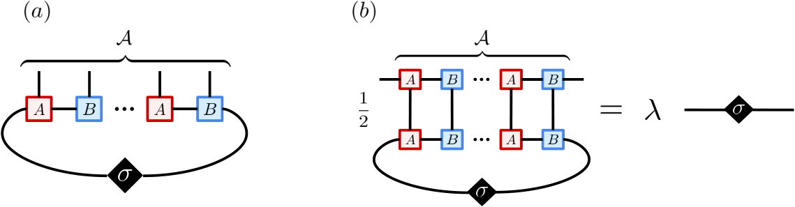
C.1 Eigenvalues of the reduced density matrix of
We prove here the result that the reduced density matrix of (in the TDL), for a (contiguous) region comprised of sites , has eigenvalues
| (30) |
Our proof will also furnish the four eigenvectors , of . The reduced density matrix, is given in Fig. 11(a).
We start by noticing that the transfer matrices of the matrices making up the MPS , have a single dominant left and right eigenvector with unit eigenvalue. In fact,
| (31) |
which we note is simply the identity matrix (a tensor) reshaped into a vector (a tensor), multiplied by the coefficient .
Thus, in the TDL, can simply be written as
| (32) |
where
see Fig. 11(b). Note the vectors act on different spaces: are vectors on the bond indices of , while correspond to vectors on the physical indices.

We consider as an ansatz
| (33) |
to be an eigenvector of , which is nothing but the original MPS but on the subregion , with appropriate boundary conditions given by the matrix , see Fig. 12(a). We parameterize this as
| (34) |
The condition to be solved then reads is an eigenvector of , that is, . It is sufficient (though not necessary) to solve the expression, written in diagrams in Fig. 12(b), for .
Consider first even . Upon evaluating Fig. 12(b), we have that
| (35) |
Thus we have the solutions
| (36) |
with corresponding . We also have to check that are orthogonal. We compute the overlap matrix
| (37) |
where is the transfer matrix equal to () for odd(even) sites. We get
| (38) |
Thus, we see that , are orthogonal (and in particular ), and that the eigenvalues sum to 1 (so ). Therefore has eigenvalues .
Next consider odd . Upon evaluating Fig. 12(b), we have that
| (39) |
Thus we have the solutions
| (40) |
with corresponding . We compute the overlap matrix and get
| (41) |
Thus, (aside from the case , but this is easily handled) we see that , are orthogonal and that the eigenvalues sum to 1, and therefore has eigenvalues , as claimed.
The entanglement entropy of the subsystem therefore admits a closed form analytic expression:
| (42) |
with , which saturates to .
C.2 Numerics: Entanglement Entropy of
While in the previous section we gave an analytic expression in the limit for the eigenvalues of the reduced density matrix of any contiguous region (thereby also yielding the entanglement entropy), in this section we leverage the MPS representation of the state to compute, numerically, for finite , its von Neumann entanglement entropy for bipartitions of the chain into two contiguous regions. (Of course, it is expected that the differences in numerical calculations and analytic expressions will be exponentially small in system size).
In order to obtain the Schmidt decomposition of the state and thereby extract the entanglement spectrum of state, the periodic MPS representation of was converted into one of two open boundary condition representations of , based on the parity of length of the subregions of the system upon bipartition, by “doubling” the PBC MPS representation, see Fig. 13.
Upon obtaining the OBC MPS representation of the state, to obtain the Schmidt decomposition of the state, we simply put the OBC representation into mixed canonical form from which we read off the singular values Schollwöck 2011.
Fig. 14 shows the half-chain von-Neumann entanglement entropy.
References
- Bloch et al. (2008) Immanuel Bloch, Jean Dalibard, and Wilhelm Zwerger, “Many-body physics with ultracold gases,” Rev. Mod. Phys. 80, 885–964 (2008).
- Lukin et al. (2019) Alexander Lukin, Matthew Rispoli, Robert Schittko, M. Eric Tai, Adam M. Kaufman, Soonwon Choi, Vedika Khemani, Julian Léonard, and Markus Greiner, “Probing entanglement in a many-body–localized system,” Science 364, 256–260 (2019).
- Kaufman et al. (2016) Adam M. Kaufman, M. Eric Tai, Alexander Lukin, Matthew Rispoli, Robert Schittko, Philipp M. Preiss, and Markus Greiner, “Quantum thermalization through entanglement in an isolated many-body system,” Science 353, 794–800 (2016).
- Langen et al. (2013) T. Langen, R. Geiger, M. Kuhnert, B. Rauer, and J. Schmiedmayer, “Local emergence of thermal correlations in an isolated quantum many-body system,” Nature Physics 9, 640 EP – (2013).
- Smith et al. (2016) J. Smith, A. Lee, P. Richerme, B. Neyenhuis, P. W. Hess, P. Hauke, M. Heyl, D. A. Huse, and C. Monroe, “Many-body localization in a quantum simulator with programmable random disorder,” Nature Physics 12, 907 EP – (2016).
- Bernien et al. (2017) Hannes Bernien, Sylvain Schwartz, Alexander Keesling, Harry Levine, Ahmed Omran, Hannes Pichler, Soonwon Choi, Alexander S. Zibrov, Manuel Endres, Markus Greiner, Vladan Vuletic, and Mikhail D. Lukin, “Probing many-body dynamics on a 51-atom quantum simulator,” Nature 551, 579 EP – (2017), article.
- Kucsko et al. (2018) G. Kucsko, S. Choi, J. Choi, P. C. Maurer, H. Zhou, R. Landig, H. Sumiya, S. Onoda, J. Isoya, F. Jelezko, E. Demler, N. Y. Yao, and M. D. Lukin, “Critical Thermalization of a Disordered Dipolar Spin System in Diamond,” Phys. Rev. Lett. 121, 023601 (2018).
- Deutsch (1991) J. M. Deutsch, “Quantum statistical mechanics in a closed system,” Phys. Rev. A 43, 2046–2049 (1991).
- Srednicki (1994) Mark Srednicki, “Chaos and quantum thermalization,” Phys. Rev. E 50, 888–901 (1994).
- Deutsch (2018) Joshua M Deutsch, “Eigenstate thermalization hypothesis,” Reports on Progress in Physics 81, 082001 (2018).
- Basko et al. (2006) D.M. Basko, I.L. Aleiner, and B.L. Altshuler, “Metal insulator transition in a weakly interacting many-electron system with localized single-particle states,” Annals of Physics 321, 1126 – 1205 (2006).
- Pal and Huse (2010) Arijeet Pal and David A. Huse, “Many-body localization phase transition,” Phys. Rev. B 82, 174411 (2010).
- Serbyn et al. (2013) Maksym Serbyn, Z. Papić, and Dmitry A. Abanin, “Local Conservation Laws and the Structure of the Many-Body Localized States,” Phys. Rev. Lett. 111, 127201 (2013).
- Huse et al. (2014) David A. Huse, Rahul Nandkishore, and Vadim Oganesyan, “Phenomenology of fully many-body-localized systems,” Phys. Rev. B 90, 174202 (2014).
- Nandkishore and Huse (2015) Rahul Nandkishore and David A. Huse, “Many-Body Localization and Thermalization in Quantum Statistical Mechanics,” Annual Review of Condensed Matter Physics 6, 15–38 (2015), https://doi.org/10.1146/annurev-conmatphys-031214-014726 .
- Abanin and Papić (2017) Dmitry A. Abanin and Zlatko Papić, “Recent progress in many-body localization,” Annalen der Physik 529, 1700169 (2017).
- Abanin et al. (2019) Dmitry A. Abanin, Ehud Altman, Immanuel Bloch, and Maksym Serbyn, “Colloquium: Many-body localization, thermalization, and entanglement,” Rev. Mod. Phys. 91, 021001 (2019).
- Calabrese et al. (2016) Pasquale Calabrese, Fabian H L Essler, and Giuseppe Mussardo, “Introduction to Quantum Integrability in Out of Equilibrium Systems,” Journal of Statistical Mechanics: Theory and Experiment 2016, 064001 (2016).
- Sutherland (2004) Bill Sutherland, Beautiful Models (World Scientific, 2004) https://www.worldscientific.com/doi/pdf/10.1142/5552 .
- Turner et al. (2018a) C. J. Turner, A. A. Michailidis, D. A. Abanin, M. Serbyn, and Z. Papić, “Weak ergodicity breaking from quantum many-body scars,” Nature Physics 14, 745–749 (2018a).
- Turner et al. (2018b) C. J. Turner, A. A. Michailidis, D. A. Abanin, M. Serbyn, and Z. Papić, “Quantum scarred eigenstates in a Rydberg atom chain: Entanglement, breakdown of thermalization, and stability to perturbations,” Phys. Rev. B 98, 155134 (2018b).
- Heller (1984) Eric J. Heller, “Bound-State Eigenfunctions of Classically Chaotic Hamiltonian Systems: Scars of Periodic Orbits,” Phys. Rev. Lett. 53, 1515–1518 (1984).
- Ho et al. (2019) Wen Wei Ho, Soonwon Choi, Hannes Pichler, and Mikhail D. Lukin, “Periodic Orbits, Entanglement, and Quantum Many-Body Scars in Constrained Models: Matrix Product State Approach,” Phys. Rev. Lett. 122, 040603 (2019).
- Shiraishi and Mori (2017) Naoto Shiraishi and Takashi Mori, “Systematic Construction of Counterexamples to the Eigenstate Thermalization Hypothesis,” Phys. Rev. Lett. 119, 030601 (2017).
- Ok et al. (2019) Seulgi Ok, Kenny Choo, Christopher Mudry, Claudio Castelnovo, Claudio Chamon, and Titus Neupert, “Topological many-body scar states in dimensions 1, 2, and 3,” arXiv e-prints , arXiv:1901.01260 (2019), arXiv:1901.01260 [cond-mat.other] .
- Choi et al. (2019) Soonwon Choi, Christopher J. Turner, Hannes Pichler, Wen Wei Ho, Alexios A. Michailidis, Zlatko Papić, Maksym Serbyn, Mikhail D. Lukin, and Dmitry A. Abanin, “Emergent SU(2) Dynamics and Perfect Quantum Many-Body Scars,” Phys. Rev. Lett. 122, 220603 (2019).
- Moudgalya et al. (2018a) Sanjay Moudgalya, Stephan Rachel, B. Andrei Bernevig, and Nicolas Regnault, “Exact excited states of nonintegrable models,” Phys. Rev. B 98, 235155 (2018a).
- Moudgalya et al. (2018b) Sanjay Moudgalya, Nicolas Regnault, and B. Andrei Bernevig, “Entanglement of exact excited states of Affleck-Kennedy-Lieb-Tasaki models: Exact results, many-body scars, and violation of the strong eigenstate thermalization hypothesis,” Phys. Rev. B 98, 235156 (2018b).
- Schecter and Iadecola (2019) Michael Schecter and Thomas Iadecola, “Weak Ergodicity Breaking and Quantum Many-Body Scars in Spin-1 XY Magnets,” arXiv e-prints , arXiv:1906.10131 (2019), arXiv:1906.10131 [cond-mat.str-el] .
- Surace et al. (2019) Federica M. Surace, Paolo P. Mazza, Giuliano Giudici, Alessio Lerose, Andrea Gambassi, and Marcello Dalmonte, “Lattice gauge theories and string dynamics in Rydberg atom quantum simulators,” arXiv e-prints , arXiv:1902.09551 (2019), arXiv:1902.09551 [cond-mat.quant-gas] .
- Moudgalya et al. (2019) Sanjay Moudgalya, B. Andrei Bernevig, and Nicolas Regnault, “Quantum Many-body Scars in a Landau Level on a Thin Torus,” arXiv e-prints , arXiv:1906.05292 (2019), arXiv:1906.05292 [cond-mat.str-el] .
- Khemani et al. (2019) Vedika Khemani, Chris R. Laumann, and Anushya Chandran, “Signatures of integrability in the dynamics of Rydberg-blockaded chains,” Phys. Rev. B 99, 161101 (2019).
- Iadecola et al. (2019) Thomas Iadecola, Michael Schecter, and Shenglong Xu, “Quantum Many-Body Scars and Space-Time Crystalline Order from Magnon Condensation,” arXiv e-prints , arXiv:1903.10517 (2019), arXiv:1903.10517 [cond-mat.str-el] .
- Lin and Motrunich (2019) Cheng-Ju Lin and Olexei I. Motrunich, “Exact Quantum Many-Body Scar States in the Rydberg-Blockaded Atom Chain,” Phys. Rev. Lett. 122, 173401 (2019).
- Ho and Radičevič (2018) Wen Wei Ho and Đorđe Radičevič, “The ergodicity landscape of quantum theories,” International Journal of Modern Physics A 33, 1830004 (2018), https://doi.org/10.1142/S0217751X18300041 .
- Fannes et al. (1992) M Fannes, B Nachtergaele, and R.F. Werner, “Finitely correlated states on quantum spin chains,” Communications in Mathematical Physics 144, 443–490 (1992).
- Weinberg and Bukov (2017) Phillip Weinberg and Marin Bukov, “QuSpin: a Python Package for Dynamics and Exact Diagonalisation of Quantum Many Body Systems part I: spin chains,” SciPost Phys. 2, 003 (2017).
- Yang (1989) Chen Ning Yang, “ Pairing and off-diagonal long-range order in a Hubbard model,” Phys. Rev. Lett. 63, 2144–2147 (1989).
- Nielsen (1999) M. A. Nielsen, “Conditions for a Class of Entanglement Transformations,” Phys. Rev. Lett. 83, 436–439 (1999).
- (40) Majorizing refers to the following situation: suppose is a pure state in a bipartite system which has a Schmidt decomposition , where and are the singular values sorted in descending order. Suppose is another state that has corresponding Schdmit decomposition with singular values , also sorted in descending order. Then for any , we say majorizes if . In particular it means for any entanglement measure .
- Kitazawa et al. (2003) Atsuhiro Kitazawa, Keigo Hijii, and Kiyohide Nomura, “An SU(2) symmetry of the one-dimensional spin-1 XY model,” Journal of Physics A: Mathematical and General 36, L351–L357 (2003).
- Schollwöck (2011) Ulrich Schollwöck, “The density-matrix renormalization group in the age of matrix product states,” Annals of Physics 326, 96 – 192 (2011), january 2011 Special Issue.