Bayesian analysis of multifidelity computer models with local features and non-nested experimental designs: Application to the WRF model
Abstract
We propose a multi-fidelity Bayesian emulator for the analysis of the Weather Research and Forecasting (WRF) model when the available simulations are not generated based on hierarchically nested experimental design. The proposed procedure, called Augmented Bayesian Treed Co-Kriging, extends the scope of co-kriging in two major ways. We introduce a binary treed partition latent process in the multifidelity setting to account for non-stationary and potential discontinuities in the model outputs at different fidelity levels. Moreover, we introduce an efficient imputation mechanism which allows the practical implementation of co-kriging when the experimental design is non-hierarchically nested by enabling the specification of semi-conjugate priors. Our imputation strategy allows the design of an efficient RJ-MCMC implementation that involves collapsed blocks and direct simulation from conditional distributions. We develop the Monte Carlo recursive emulator which provides a Monte Carlo proxy for the full predictive distribution of the model output at each fidelity level, in a computationally feasible manner. The performance of our method is demonstrated on a benchmark example, and compared against existing methods. The proposed method is used for the analysis of a large-scale climate modeling application which involves the WRF model.
Keywords: Augmented hierarchically nested design, Binary treed partition, Gaussian process, Collapsed MCMC
1 Introduction
Understanding the behavior as well as the underlying mechanisms of real systems such as physical procedures is central to many applications such as weather forecasting. Direct investigation of the real system is often impossible due to limited resources, and hence it is simulated by computer models aiming at reproducing the real system’s behavior with high accuracy. Our case study involves an expensive computer model which requires a significant amount of resources to perform a single run; and hence, only a limited number of simulations can be performed. Gaussian process (GP) regression models (Sacks et al. 1989) are statistical models that allow the emulation of the computer model output by using only a few runs of the computer model.
Computer models are often able to run at different levels of fidelity, sophistication, or resolution. As high fidelity runs are usually more expensive, collecting data by simulating the model at different fidelity levels is preferred for a given budget of resources. Statistical inference is preferable to be made against the whole simulated data-set, and thus account for across fidelity level dependence, rather than against simulation data-sets associated with individual fidelity levels (Kennedy and O’Hagan 2000). Assume there are available deterministic computer models aiming at simulating the same real system. The models are ordered by ascending fidelity level . Let denote the output function of the computer model with respect to a -dimensional input . Autoregressive co-kriging assumes
| (1) |
where , , are independent unknown functions a priori modeled as Gaussian processes. Here, is the location discrepancy function (representing a local adjustment from to ), and is the scale discrepancy (representing a scale change from to for ). Discrepancy terms, and , can be thought of as accounting for ‘missing’ or ‘misrepresented’ physical properties in the lower fidelity computer model with respect to the higher one . Model (1) is induced by the Markovian condition ; i.e, there is nothing more to learn about from for any given is known.
A number of important variations of the autoregressive co-kriging have been proposed. Qian and Wu 2008 considered the scale discrepancy as a function of the input space by casting it as a GP. In practice, this approach is applicable to problems with only two fidelity levels, as the computational overhead caused by using more fidelity levels is increased dramatically. Gratiet 2013; Gratiet and Garnier 2014 modeled the scale discrepancy as an expansion of bases defined on the inputs, and presented conditional conjugate priors which lead to standard conditional posterior distributions for the unknown coefficients of the expansion. However, casting the scale discrepancy as a basis expansion may require an undesirably large number of bases in order to describe small scale discrepancies; while it cannot represent discontinuities and sudden changes. Furthermore, this may aggravate non-identifiability between the scale and additive discrepancies. Perdikaris et al. 2015 proposed a machine learning framework, which uses sparse precision matrices of Gaussian-Markov random fields introduced by Lindgren et al. 2011. This facilitates computations that leverage on the sparsity of the resulting discrete operators. Perdikaris et al. 2017 relaxed the auto-regressive structure by using deep learning ideas, however the computational demands to train the model are significantly increased. The aforementioned developments require hierarchically nested experimental designs for computational reasons, otherwise the computational demands become impractical. This constraint prevents their practical implementation on a number of important real problems where the available data-set is not based on such nested designs.
Our case study and motivation is a real world application that involves the Weather Research and Forecasting (WRF) regional climate model (Skamarock et al. 2008). WRF is an expensive computer model that allows the use of different resolutions leading to different fidelity levels. We consider the WRF with the Rapid Radiative Transfer Model for General Circulation Model (Pincus et al. 2003), with the Kain-Fritsch convective parametrisation scheme (KF CPS) (Kain 2004), and with five input parameters, while we are interested in the average precipitation as an output. The available simulations were generated by running WRF at two resolution levels, km and km grid spacing. The fidelity of the simulations increases when the grid spacing gets finer. The available simulations have not been generated based on a hierarchically nested design, while it is not possible to re-run the expensive computer model in our facilities and generate simulations based on such a design due to the high computational cost required. The aforesaid co-kriging methods cannot be implemented directly due to the lack of nested design, and hence new developments are required. We are interested in designing an accurate emulator that aggregates all the available simulations as well as represents features of the WRF. Previous research in (Yan et al. 2014; Yang et al. 2012) suggested that discrepancies between the two levels may depend on the five inputs of the KF CPS. Interest also lies in better understanding how different grid spacing affects the discrepancies in WRF with respect to the input parameters. Existing co-kriging methods do not model/account for such behaviors, thus suitable extensions must be introduced.
We propose the Augmented Bayesian Treed co-kriging (ABTCK); a fully Bayesian method for building multifidelity emulators of computer models that extends the scope of co-kriging mainly in two ways. The proposed method is able to address applications where the available training data-set has not necessarily been generated according to a hierarchically nested experimental design. To achieve this, we introduce a suitable imputation mechanism that augments the original data-set with uncertain quantities which can be thought of as missing data from a hypothetical complete data-set generated based on an hierarchically nested design. The proposed imputation allows the specification of conditional conjugate priors, and analytic integration of a large number of dimensions from the posterior. Moreover, our method is able to account for non-stationary, and possible discontinuities. This is achieved by suitably specifying the statistical model as a combination of computationally convenient and simple GP models by using a binary treed partition which a priori follows a process similar to (Chipman et al. 1998; Gramacy and Lee 2008). The additional flexibility of the proposed model aims at producing more accurate predictions as well as providing an insight of the model discrepancies. To facilitate inference, we propose a reversible jump Markov chain Monte Carlo (RJ-MCMC) implementation, tailored to the proposed model, that involves an efficient MCMC sampler which operates on the joint space of the missing data and the parameters, and consists of collapsed blocks. Due to the augmentation, the MCMC loop consists of local RJ updates operating on a lower dimensional state space and producing more acceptable proposals, and a block simulating the missing data directly from the conditionals. Finally, we propose the Monte Carlo recursive emulator, as an alternative to those in (Kennedy and O’Hagan 2000; Gratiet and Garnier 2014; Gratiet 2013), which is able to provide fully Bayesian posterior predictive inference even with non-nested designs while keeping the computational cost lower than the others.
2 The Augmented Bayesian Treed co-Kriging
We describe the development of our Augmented Bayesian treed co-kriging model (ABTCK) which extends the scope of co-kriging to applications with non-nested designs and/or non-stationary model outputs.
2.1 Treed auto-regressive co-kriging
To account for non-stationarity we consider an known partition of the input space , whose sub-regions are assumed to be homogeneous in the sense that a co-kriging model (1) can be defined independently at each sub-region, i.e.
| (2) |
such that input dependencies are represented accurately enough by parameterizing the unknown scale discrepancies , location discrepancies , and output functions with computationally convenient forms.
We cast as a binary tree partition with rectangular sub-regions , for , determined by a binary tree . This specification adds structure to the model for the sake of computational convenience, however it can still provide a reasonable approximation to the reality. Binary treed partitioning has been successfully used in other problems (Denison et al. 1998; Chipman et al. 1998; Gramacy and Lee 2008; Pratola et al. 2017; Konomi et al. 2017; Karagiannis et al. 2017). To account for the uncertainty about , we use the binary tree process prior of Chipman et al. 1998 specified as
| (3) |
where denotes the set of external nodes corresponding to sub-regions of the partition and denotes the internal nodes. Tree has origin denoting the whole input space , while each node represents a sub-region of the input space. Each node splits with probability where is the depth of , controls the balance of the shape of the tree, and controls the size of the tree. The splits are preformed based on a random splitting rule following a distribution .
We specify mutually independent Gaussian processes (GP) priors for , and
| (4) | ||||
| (5) |
for , to account for their uncertainty. Given a suitable partition for the model (2), we can use simple and computationally convenient functions to model , , and . We specify square exponential correlation function in separable form , however more sophisticated ones can be used (Williams and Rasmussen 2006). The mean functions are parametrized as basis expansions , where is a vector of basis functions and are vectors of coefficients, at fidelity level , and sub-region . The unknown functions are modeled as low degree basis expansions where are polynomial bases and are uncertain coefficients. Modeling , and as basis expansions facilitates the specification of conjugate priors and leads to computational savings given a suitable treatment in the likelihood.
2.2 Conditional-conjugacy via augmentation
We do not require the available experimental design to be hierarchically nested, unlike existing co-kriging methods (Kennedy and O’Hagan 2000; Gratiet 2013). Namely, if denotes the available a training data-set with output values at the experimental design of size at fidelity level , it may be for some . This realistic generalization prevents the direct specification of priors conjugate to the Gaussian likelihood , and hence makes the Bayesian computations prohibitively expensive. In such cases, direct implementation of existing co-kriging methods would require the inversion of large covariance matrices with size for the computation of the likelihood, and possibly the use of Metropolis-Hastings operations in high-dimensional state spaces which would lead to practically infeasible computations. The introduction of the binary partition aggregates this issue as it increases the dimensionality of the posterior by introducing additional unknown parameters ; this necessitates the specification of conjugate priors.
We address this issue by properly imputing the observed data with uncertain quantities, that can be thought of as missing data of a hierarchically nested experimental design able to induce a conditional independence that enables the specification of conjugate priors, facilitates tractability of posterior marginals and conditionals, and allows the design of efficient MCMC implementations, while it leads to the same Bayesian inference as if we had considered the original data-set only.
Augmentation
Let be the observed data-set with output values and design at sub-region and fidelity level . Assume sets of points and such that with , and where for . It is easy to check that , and that is hierarchically nested; i.e. . By construction, is the smallest collection of sets of input points required to be added to the original design in order to obtain a hierarchically nested experimental design . Let be the missing output values of the computer model at the corresponding input points in . We refer to as missing data-set, and as complete data-set, where is the complete experimental design, and are the output model values at input points in .
The joint distribution of given the parameters is
| (6) |
where each conditional is a Gaussian distribution with mean , and covariance . Here, denotes the Hadamard product. The join distribution of can be factorized as in (6) because the proposed augmentation artificially creates a hierarchically nested design which due to the Markovian condition of (2) induces the required conditional independence. The computation of the augmented likelihood (6) is broken down into that of Gaussian densities requiring the inversion of covariance matrices. Otherwise, we would be unable to factorize (6) and we would be required to invert a larger covariance matrices with sizes .
Priors
To account for the uncertainty about unknowns , we specify a prior factorized as
| (7) |
We assign Normal-inverse-gamma prior distributions on such as
which are conjugate to the conditionals in augmented likelihood (6). This allows the analytic marginalization of the posterior and leads to important computational benefits discussed in Section 2.3. Without augmentation, we would be unable to specify conjugate priors for the actual likelihood, and computations for learning would be impractical. Elicitation of the priors is performed according to (Oakley 2002; Brynjarsdóttir and O’Hagan 2014). Weakly informative Jeffreys’ priors are obtained by adjusting , , and to be close to zero, and for , and . Here, are proper priors chosen by the researcher.
The posterior distribution of ABTCK model is
| (8) |
admits the posterior of interest as marginal by construction, and hence leads to the same Bayesian analysis.
2.3 Bayesian inference and computations
We design a RJMCMC sampler, targeting the augmented posterior (8), that involves a random permutation scan of blocks updating , , and . The blocks are collapsed to avoid undesired high MC standard errors due to the originally high-dimensional sampling space (Liu 1994). The sampler is computationally efficient as it breaks down the inversion of covariance matrices and involves parallel sampling at different sub-regions and fidelity levels . Details regarding the MCMC blocks are explained below.
Update
The full conditional posterior of , after integrating out ’s from the joint posterior (8), is a Normal distribution with mean and covariance matrix
| (9) | ||||
where , for and . The functions , , and are given in the Appendix A. We observe that, updating missing data takes into account information from the lower level , the current level , and higher level by interpolating the associated moments. For instance, (and ) provide information about the location of from levels , (and levels , ). Hence, each update interpolates not only across the input space at an individual fidelity level but also across the fidelity levels. Simulation of can be performed in parallel for which is a computational benefit, and it can be suppressed if .
Elaborating further into specific cases of the above imputation, if levels and do not share any design points at all, at sub-region , i.e., , then , and . This implies that, given weak priors on are specified, i.e. , the update of missing obtains information from the upper level which entirely relies on the observed output and not from the discrepancy terms and of the two levels. If levels and share design points, , the extra structure of the equations of and in (27) and (26) (see Appendix A) can be interpreted as the factor quantifying the discrepancy between levels and . Finally, we can see that when the correlation between the two levels and , at sub-region , is weak, e.g. , the missing data update resembles the prediction relying only on the information from the current level . Based on these observations, it may be preferable to consider designs with some overlap at adjacent levels not only for computational convenience but also for modeling reasons. However, a theoretical proof of this statement is out of our scope.
Update
To update , we propose a mixture of the Markov transitions targeting the augmented marginal posterior whose density is proportional to
| (10) | ||||
| (11) |
where . Functions and are given in (23) and (24) in Appendix A. The Markov transitions are based on the operations change, swap, rotate, and grow & prune, introduced by (Chipman et al. 1998; Gramacy and Lee 2008). The first three operations are Metropolis-Hastings algorithms (Hastings 1970) whose implementation is straightforward. The grow & prune operations are local reversible jump (RJ) transitions and further specification is required.
The grow operation performing a transition from state to works as follows. We randomly select an external node and assume it corresponds to a sub-region , data-set , and parameters though the augmented statistical model. We propose node to split into two new child nodes and according to the splitting rule in prior (7), and we denote the proposed tree as . Nodes and correspond to disjoint sub-regions and (with ), data-sets and , and parameters and , respectively. Randomly, one of the parameters or inherits the values from the parent ones; e.g., . The values of the other parameter are proposed by simulating from a probability distribution; e.g., , such as the corresponding priors. The rest elements of inherit their values from . The proposed transition is accepted with probability where
| (12) |
is the set of growable nodes in tree , and is the set of prounable nodes in tree . The prune operation, performing a transition from state to , is fully defined as the reverse operation of the Grow one, and is accepted with probability .
Due to the proposed augmentation in Section 2.2, we are able to analytically integrate out a potentially high-dimensional parameter vector from the joint density (8), and hence design local RJ moves targeting the marginal . The benefit from this collapsed update is that the proposed RJ algorithm operates on a lower dimensional state space, which allows for shorter and more acceptable jumps in practice. If necessary, grow and prune operations can be further improved by using the annealing mechanism of Karagiannis and Andrieu 2013.
Update
The conditional posterior has the form
| (13) | ||||
| (14) | ||||
| (15) | ||||
| (16) | ||||
| (17) |
where the hatted quantities are given in (21)-(23) of Appendix A.
Conditional distributions (13)-(16) can be sampled directly, and in parallel for different . Sampling from the full conditional of ’s (13) and (14) is not necessary and can be ignored from the MCMC swap if prediction is the only concern of the analysis. This is because ’s can be analytically integrated out from the proposed emulator in Section 2.4. Alternatively, ’s can be sampled outside the MCMC swap (13) and (14) by conditioning.
Updating by simulating from is not necessary in theory, as it is updated in block , however it improves mixing in practice. The marginal posterior (17) cannot be sampled directly. Conditional independence in (10) implies that can be simulated by running in parallel Metropolis-Hastings algorithms each of them targeting distributions with densities proportional to (11).
2.4 Posterior analysis and emulation
Assume there is available a MCMC sample generated from the RJMCMC sampler in Section 2.3, and let denote the partition corresponding to tree . Central Limit Theorem can be applied to facilitate inference as the proposed sampler is aperiodic, irreducible, and reversible (Roberts et al. 2004).
The proposed procedure ABTCK allows inference to be performed for the missing output values at input points in . Inference on can be particularly useful when the computer model has been unable to generate simulations at these input points due to numerical crash or limitations. The marginal posterior distribution of , along with its expectations, can be approximated via standard Monte Carlo (MC) using the generated samples at each level . Alternatively, point estimates of at can be approximated by the more accurate Rao-Blackwell MC estimator where is the -th MCMC realization of (9).
A Monte Carlo recursive emulator able to facilitate fully Bayesian predictive inference on the output at untried input points at every fidelity level can be derived. The conditional distribution inherits a conditional independence similar to (6) due to the augmentation of the data with that allows to be analytically integrated out with respect to (13)-(16). Hence the distribution of , at sub-region , is calculated as
| (18) | ||||
| (19) |
where the conditionals are Student-T processes (STP) with
for , and for and for a set . An MCMC sample from the predictive distribution of , at can be obtained by simulating (18)-(19) given the sample values . This allows the computation of a Monte Carlo approximation of the emulator of ], and its moments, at any fidelity level . The conditional independence in the predictive distribution (18) and (19) results because of our imputation strategy.
The proposed emulator accounts for non-stationariy and discontinuity by aggregating simpler GP emulators in a Bayesian model averaging manner, while it integrates uncertainty regarding the unknown ‘missing data’ and parameters. It is computationally preferable compared to existing co-kriging one (Kennedy and O’Hagan 2000; Gratiet 2013) because it allows the parallel inversion of smaller covariance matrices with sizes while the others require the inversion of a large co-variance matrix of size . Moreover, it is able to recover the whole predictive distribution and its moments, unlike the derivation in Gratiet and Garnier 2014 where only the predictive mean and variance are derived recursively. More importantly, it is able to be applied in problems where the training data set is not hierarchically nested, while its competitors cannot.
2.5 Further particulars
Two novel co-kriging procedures can be distinguished as special cases of the proposed ABTCK. In applications where the design is non hierarchically nested, but the computer model outputs can be assumed as stationary, one can consider to drop the partitioning by setting and suppressing the MCMC update . We will refer to this reduced version of ABTCK as Augmented Bayesian co-kriging (ABCK). Unlike standard co-kriging, our ABCK can be applied with non-nested designs as it makes the computations for training the Bayesian model or computing the emulator practically feasible. In fact, the proposed augmentation strategy separates the posterior into conditionally independent quantities and allows closed form inference for the majority of the hyper-parameters. Another special case is where the design is hierarchically nested but the model outputs present non-stationarity, the imputation mechanism can be dropped by setting and suppressing the update . We will refer to this reduced version of ABTCK as Bayesian treed co-kriging (BTCK). In such a case, BTCK can be preferable to the standard co-kriging as it can model the aforesaid stationarity by properly combining simple stationary GPs.
The computational complexity of the proposed ABTCK compared to existing co-kriging methods is reduced in two ways: a) by breaking the emulation into parts via the partitioning, and b) by breaking the emulation into parts via the recursively prediction procedure. In ABTCK the computational complexity of evaluating the augmented likelihood or the predictive distribution is in sequential computing environments, while it can be further reduced to in parallel computing environments since operations at each can be performed in parallel. Under non-hierarchical designs, our ABCK (assuming the partitioning is dropped) requires for the evaluation of the augmented likelihood or the Monte Carlo emulator which is smaller than required by (Kennedy and O’Hagan 2000; Gratiet et al. 2014) for the evaluation of the associated likelihoods since .
3 Case study
We examine the performance of the proposed augmented Bayesian treed co-kriging (ABTCK) method as well as its special case ABCK on a benchmark example. Consider functions
| (20) |
presented in Figure 1, which are assumed to be output functions of computer models and with being more accurate but slower to run than . By expressing (20) as (1), it can be seen that the discrepancy functions and change over .


We pretend that the equations (20) are unknown, and we generate the observed data-set based on a randomly selected non-hierarchically nested design . For level , the observed data are generated by employing a Latin Hypercube Sampling (LHS) (McKay et al. 1979) to specify design points , and computing the corresponding observations from (20). For level , the observations are generated likewise by specifying input values via LHS such that .
We study the effectiveness of the treed partition mechanism in the co-kriging setting by comparing two versions of the proposed method, the ABTCK equipped with a partitioning mechanism and the ABCK where that mechanism is suppressed. Existing co-kriging methods in (Kennedy and O’Hagan 2000; Qian and Wu 2008; Gratiet 2013) require hierarchically nested designs and cannot be implemented in this setting.
Regarding ABTCK, we consider weakly informative priors with hyper-parameters , , , and a mixture prior of Gamma distributions for distributing the prior mass on areas of smaller and larger values (Gramacy and Lee 2008). The scale discrepancy is parametrised as a zero-degree basis expansion . The tree process prior has hyper-parameters and . To make the comparison fair, ABCK shares the same settings as ABTCK. To learn the unknown parameters, we generate a MCMC sample by running the sampler for iterations and discarding the first sampled values as burn-in.
Figures 2a and 2b present the predictive means of as functions of the inputs for ABCK and ABTCK respectively. We observe that the predictive mean produced by ABTCK is closer to the exact than that produced by ABCK. ABTCK has produced a MSPE while the stationary ABCK has produced a MSPE , where MSPE is computed based on a grid of input values. This suggests that the treed partitioning mechanism, as implemented in our ABTCK, is able to successfully capture and model the non-stationarity, and hence produce more accurate predictions, in the multifidelity setting.


The algorithms have been implemented in MATLAB R2017b and run on a computer with specs: IntelCore™i7-7700K CPU @ 4.20GHz 8, and 62.8 GiB RAM but in a sequential fashion. The computation time of training ABTCK was around two times quicker than ABCK. This is because ABTCK requires the inversion of smaller covariance matrices than ABCK in the MCMC sampling due to the partitioning. It appears that the computational overhead introduced by the RJ operation is dominated by the computational gain due to the partition and subsequent inversion of smaller matrices.
In Figure 3, we present the Monte Carlo approximation of the posterior mean of the scalar discrepancy produced by the ABTCK. We observe that ABTCK has recovered a representation of the scalar discrepancy which suggests that changes value. In contrast, ABCK produces a posterior scalar discrepancy which is equal to and constant throughout the input space due to the lack of partitioning.

4 Application to large-scale climate modeling
We consider the Advanced Research Weather Research and Forecasting Version 3.2.1 (WRF Version 3.2.1) climate model (Skamarock et al. 2008) constrained in the geographical domain and over the Southern Great Plains (SGP) region, and we concentrate on the average precipitation response over the area.
We briefly discuss the set-up of the WRF computer model, however more details can be found in (Yan et al. 2014). WRF is employed with the Morrison 2-moment cloud microphysics scheme (Morrison et al. 2005) and the Kain-Fritsch convective parametrisation scheme (KF CPS) (Kain 2004) as in (Yang et al. 2012). The most critical parameters (Yang et al. 2012; Yan et al. 2014) of the KF scheme are: the coefficient related to downdraft mass flux rate that takes values in range ; the coefficient related to entrainment mass flux rate that takes values in range ; the maximum turbulent kinetic energy in sub-cloud layer () that takes values in range ; the starting height of downdraft above updraft source layer (hPa) that takes values in range ; and the average consumption time of convective available potential energy that takes values in range . The ranges of the KF CPS parameters are quite wide and hence cause higher uncertainties in climate simulations due to the non linear interactions and compensating errors of the parameters (Gilmore et al. 2004; Murphy et al. 2007; Yang et al. 2012). We consider the Rapid Radiative Transfer Model (RRTMG) for General Circulation Models (Mlawer et al. 1997) as a more accurate radiation scheme for the geological domain of interest. Here, we are interested in modeling the average precipitation with respect to the five parameters of the convective parametrisation scheme.


The available simulations were generated by running WRF model times at two resolution levels; model runs for km grid spacing and model runs km grid spacing. The fidelity of the simulations increases when the grid spacing gets finer. The available simulations have been generated based on a non hierarchically nested design at the five input parameters (Figure 4). The samples have been generated via a simulated stochastic approximation annealing (SSAA) calibration algorithm published in (Yan et al. 2014). As the SSAA procedure progresses, the sampling range of each parameter gradually narrows as shown in Figure 4. Different resolutions give different narrowing range on the input space. Due to the high cost, it is not possible to re-run the expensive WRF model in order to generate simulations based on a hierarchically nested design as existing co-kriging methods require. As discussed in (Yang et al. 2012; Yan et al. 2014) the discrepancies between the two fidelity levels may depend on the five inputs, however no formal statistical analysis have been performed. The atmospheric humidity at all levels is lower in the fine resolution than coarse resolution, and the drier atmosphere may result from more condensation (so more precipitation generated) which consumes more moisture at the finer resolution. The explicit precipitation increases with spatial resolution because more clouds are resolved at finer resolution. Moreover, interest lies in better understanding how different grid spacing affects the discrepancies in WRF with respect to the input parameters.
We implement the ABTCK proposed method to analyze the data set. To make comparisons regarding the necessity of the treed partition as implemented in our method in the multi-fidelity framework, we consider the ABCK, namely the ABTCK without the partition mechanism. It is important to notice that existing co-kriging techniques cannot be implemented in this application because the available experimental design is not hierarchically nested. We compare our proposed ABTCK and ABCK against the standard GP emulator trained against the observed data of the higher fidelity level only, to demonstrate the importance of using co-kriging in multi-fidelity problems even under non-hierarchically nested designs. To ensure fair comparison, the covariance function family is the same for all three methods, namely: separable square exponential covariance functions. Regarding the prior model, for the correlation parameters, we assign Gamma mixture priors distributing the mass on areas of smaller and larger values; for the binary treed partition priors, we consider hyper-parameters and ; and for the rest parameters we consider weak informative priors as , , , and . Regarding the grow & prune update, we use the prior distributions as the dimensional matching proposals . We have re-scaled the input space for the five parameters to be between in order to be able to use the same proposal distribution for all ’s. To train the model, we run the MCMC sampler for iterations from which we discard as burn in.
We randomly choose half of the simulations as the evaluation data-set, and we use the rest simulations as the training data-set. To account for the variation due to the stochastic nature of the procedures and the bias due to the evaluation set, we perform realizations for each procedure with different evaluation sets each time.The comparison is performed based on the MSPE, the coverage probability of the equal-tail credible interval (CVG(95%)), the Nash-Sutcliffe model efficiency coefficient (NSME), and the computational time. The average of each of these quantities for the three methods is presented in Table 1. To give a better representation of the variation, we also present the boxplots of the MSPEs produced from simple GP, ABCK, and ABTCK in Figure 5.
| MSPE | CVG(95%) | NSME | Time(sec) | |
|---|---|---|---|---|
| GP | 0.2118 | 0.613 | 0.31 | 368 |
| ABCK | 0.1205 | 0.840 | 0.79 | 1804 |
| ABTCK | 0.0974 | 0.945 | 0.87 | 1240 |


Both ABCK and ABTCK outperform the simple GP by a large margin in terms of accuracy and constructing more accurate credible intervals. The mean MSPE and NSME for both ABCK and ABTCK is less than half of that produced by the simple GP. Moreover, we observe that ABTCK produced smaller MSPE and NSME than ABCK for all the realizations, and hence ABTCK has produced more accurate results than ABCK. The average MSPE from ABCK is while the average MSPE from ABTCK is , which implies an improvement about on the MSPE when we consider the partition and hence we take into account non-stationarity. The prediction accuracy is also reflected in the NSME. The average NSME of the ABTCK is closer to one than both ABCK and GP. Based on the calculated average CVG(95%), the ABTCK produced the best representation of the uncertainty. Not only the ABTCK produced more accurate predictions but also it gave a better picture of the uncertainty associated with these predictions. Moreover, the average number of the generated subregions (tree external nodes) varies from to . This evidence supports the use of ABTCK instead of ABCK and hence the use of a non-stationary process via partitioning. The maximum MSPE difference was and it was observed in the realization corresponding to the evaluation dataset (left out simulations) which was more scattered than the rest in a wider range of the input space. This was almost improvement in the MSPE. When the majority of the left out simulations are close to the narrowing range of the simulated input space these differences become smaller but yet significant. Finally, it is important to notice that the computational time in ABTCK is approximately two third of the computational time in ABCK. This means that the improvements on the prediction and uncertainty described above come in a lower computational cost. It is worth noticing that we can further reduce the computational cost of ABTCK if we utilize parallel computing as explained in section 2.5.
In Figure 6, we plot the simulated precipitation from WRF at high fidelity, the predicted average precipitation produced from ABTCK, from ABCK, and from simple GP with respect to the downdraft mass flux rate and the coefficient related to entrainment mass flux rate . Precisely, we present the case corresponding to realizations with the highest MSPE differences between ABTCK and GP. It is obvious that the GP is not able to capture the variation in the central part of the plot where observations for high level model are sparse. Both ABCK and ABTCK are able to capture that variation with the help from the low fidelity model. regarding the differences: we observe that ABCK produced a smoother representation of the precipitation, however ABTCK was able to more accurately represent the local features. This is especially noticeable on the middle of Figure 6. The prediction is much improved over the whole left out simulation runs even in the clustered small range.
5 Conclusions and further work
We built a Bayesian emulator for the Weather Research and Forecasting (WRF) model. The proposed method, called Augmented Bayesian Treed Autoregressive Co-Kriging, extends the scope of the co-kriging methods. First our procedure can be implemented in problems where the experimental design is not necessarily hierarchically nested while keeping the computational demands low. This overcomes the difficulty of existing co-kriging methods which require hierarchically nested designs in order to keep the computations practically feasible. Secondly, our method can account for non-stationarity, and potential discontinuity, in the output of the computer models without the need to specify complicated or problem specific GP priors, in the multifidelity setting. Finally, we propose the use of a Monte Carlo recursive emulator which can recover the predictive distribution of the computer model output at every level, and can be used with non-hierarchically nested designs as well, while keeping the computational cost lower than the existing emulators as it requires operations with smaller matrices.
We analyzed the Weather Research and Forecasting (WRF) simulator using the Kain-Fritsch convective parametrisation scheme by using our novel procedure. This is a large-scale climate modeling application where the available simulations are performed at different fidelity levels at non hierarchically nested designs. Our method discovered non-stationarity in the WRF output precipitation with respect to the KFC input parameters. We observed that the use of Bayesian treed partition in the co-kriging framework as utilized in our method is able to provide more accurate predictions than ignoring it. For instance, in the WRF application we observed the use of the partition was able to reduce the MSPE around on average when we compared the ABTCK with the ABCK where the partitioning was dropped out. In our simulation example considering non-nested designs, we observed that the augmentation mechanism was able to recover the model output accurately enough.
The procedure can be modified to involve a basis selection mechanism for of and of at different input sub-regions , by properly specifying spike-and-slab priors on and and calculating Gibbs updates. One can use the fixed hyper-parameters of the latent treed process to control or mitigate possible non-identifiability between the discrepancy functions, by setting and meaningful priors on in the sense of (Brynjarsdóttir and O’Hagan 2014). The rational is that the treed prior can act as a penalty favoring simpler partitions, which can mitigate the competition between the two discrepancies. An extension of ABTCK would be to specify different partitions for , , , which may lead to a more flexible model, however, it is not clear if conditional posteriors can still be marginalized to keep the computational demands feasible. The authors are currently working on a sequential design procedure with multifidelity simulations that take into account non-hierarhically nested designs.
References
- Brynjarsdóttir and O’Hagan (2014) Brynjarsdóttir, J. and O’Hagan, A. (2014), “Learning about physical parameters: The importance of model discrepancy,” Inverse problems, 30, 114007.
- Chipman et al. (1998) Chipman, H., George, E., and McCulloch, R. (1998), “Bayesian CART Model Search,” Journal of the American Statistical Association, 93, 935–960.
- Denison et al. (1998) Denison, D., Mallick, B., and Smith, A. (1998), “A Bayesian CART Algorithm,” Biometrika, 85, 363–377.
- Gilmore et al. (2004) Gilmore, M. S., Straka, J. M., and Rasmussen, E. N. (2004), “Precipitation uncertainty due to variations in precipitation particle parameters within a simple microphysics scheme,” Monthly weather review, 132, 2610–2627.
- Gramacy and Lee (2008) Gramacy, R. B. and Lee, H. K. H. (2008), “Bayesian treed Gaussian process Models with an application to computer modeling,” Journal of the American Statistical Association, 103, 1119–1130.
- Gratiet (2013) Gratiet, L. L. (2013), “Bayesian analysis of hierarchical multifidelity codes,” SIAM/ASA Journal Uncertainty Quantification, 1, 244–269.
- Gratiet et al. (2014) Gratiet, L. L., Cannamela, C., and Iooss, B. (2014), “A Bayesian Approach for Global Sensitivity Analysis of (Multifidelity) Computer Codes,” SIAM/ASA Journal on Uncertainty Quantification, 2, 336–363.
- Gratiet and Garnier (2014) Gratiet, L. L. and Garnier, J. (2014), “Recursive co-kriging model for design of computer experiments with multiple levels of fidelity,” International Journal for Uncertainty Quantification, 4, 365–386.
- Hastings (1970) Hastings, W. K. (1970), “Monte Carlo sampling methods using Markov chains and their applications,” Biometrika, 57, 97–109.
- Kain (2004) Kain, J. S. (2004), “The Kain-Fritsch convective parameterization: an update,” Journal of Applied Meteorology, 43, 170–181.
- Karagiannis and Andrieu (2013) Karagiannis, G. and Andrieu, C. (2013), “Annealed importance sampling reversible jump MCMC algorithms,” Journal of Computational and Graphical Statistics, 22, 623–648.
- Karagiannis et al. (2017) Karagiannis, G., Konomi, B. A., and Lin, G. (2017), “On the Bayesian calibration of expensive computer models with input dependent parameters,” Spatial Statistics.
- Kennedy and O’Hagan (2000) Kennedy, M. and O’Hagan, A. (2000), “Predicting the output from a complex computer code when fast approximations are available,” Biometrika, 87, 1–13.
- Konomi et al. (2017) Konomi, B. A., Karagiannis, G., Lai, K., and Lin, G. (2017), “Bayesian Treed Calibration: An Application to Carbon Capture With AX Sorbent,” Journal of the American Statistical Association, 112, 37–53.
- Lindgren et al. (2011) Lindgren, F., Rue, H., and Lindström, J. (2011), “An explicit link between Gaussian fields and Gaussian Markov random fields: the stochastic partial differential equation approach,” Journal of the Royal Statistical Society, Series B (Statistical Methodology), 74, 423–498.
- Liu (1994) Liu, J. S. (1994), “The collapsed Gibbs sampler in Bayesian computations with applications to a gene regulation problem,” Journal of the American Statistical Association, 89, 958–966.
- McKay et al. (1979) McKay, M., Beckman, R., and Conover, W. (1979), “A comparison of three methods for selecting values of input variables in the analysis of output from a computer code,” Technometrics, 21, 239–245.
- Minasny and McBratney (2006) Minasny, B. and McBratney, A. B. (2006), “A conditioned Latin hypercube method for sampling in the presence of ancillary information,” Computers & geosciences, 32, 1378–1388.
- Mlawer et al. (1997) Mlawer, E. J., Taubman, S. J., Brown, P. D., Iacono, M. J., and Clough, S. A. (1997), “Radiative transfer for inhomogeneous atmospheres: RRTM, a validated correlated-k model for the longwave,” Journal of Geophysical Research: Atmospheres (1984–2012), 102, 16663–16682.
- Morrison et al. (2005) Morrison, H., Curry, J., and Khvorostyanov, V. (2005), “A new double-moment microphysics parameterization for application in cloud and climate models. Part I: Description,” Journal of the Atmospheric Sciences, 62, 1665–1677.
- Murphy et al. (2007) Murphy, J. M., Booth, B. B., Collins, M., Harris, G. R., Sexton, D. M., and Webb, M. J. (2007), “A methodology for probabilistic predictions of regional climate change from perturbed physics ensembles,” Philosophical Transactions of the Royal Society of London A: Mathematical, Physical and Engineering Sciences, 365, 1993–2028.
- Oakley (2002) Oakley, J. (2002), “Eliciting Gaussian process priors for complex computer codes,” Journal of the Royal Statistical Society: Series D (The Statistician), 51, 81–97.
- Perdikaris et al. (2017) Perdikaris, P., Raissi, M., Damianou, A., Lawrence, N., and Karniadakis, G. E. (2017), “Nonlinear information fusion algorithms for data-efficient multi-fidelity modelling,” Proceedings of the Royal Society A: Mathematical, Physical and Engineering Sciences, 473, 20160751.
- Perdikaris et al. (2015) Perdikaris, P., Venturi, D., Royset, J., and Karniadakis, G. (2015), “Multi-fidelity modelling via recursive co-kriging and Gaussian–Markov random fields,” Proc. R. Soc. A, 471, 20150018.
- Pincus et al. (2003) Pincus, R., Barker, H. W., and Morcrette, J.-J. (2003), “A fast, flexible, approximate technique for computing radiative transfer in inhomogeneous cloud fields,” Journal of Geophysical Research: Atmospheres (1984–2012), 108.
- Pratola et al. (2017) Pratola, M., Chipman, H., George, E., and McCulloch, R. (2017), “Heteroscedastic BART Using Multiplicative Regression Trees,” arXiv preprint arXiv:1709.07542.
- Qian and Wu (2008) Qian, P. Z. and Wu, C. J. (2008), “Bayesian hierarchical modeling for integrating low-accuracy and high-accuracy experiments,” Technometrics, 50, 192–204.
- Roberts et al. (2004) Roberts, G. O., Rosenthal, J. S., et al. (2004), “General state space Markov chains and MCMC algorithms,” Probability surveys, 1, 20–71.
- Sacks et al. (1989) Sacks, J., Welch, W. J., Mitchell, T. J., and Wynn, H. P. (1989), “Bayesian Design and Analysis of Computer Experiments: Use of Derivatives in Surface Prediction,” Statistical Science, 4, 409–435.
- Skamarock et al. (2008) Skamarock, W. C., Klemp, J. B., Dudhia, J., Gill, D. O., Barker, M., Duda, K. G., Huang, X. Y., Wang, W., and Powers, J. G. (2008), “A description of the Advanced Research WRF Version 3,” Tech. rep., National Center for Atmospheric Research.
- Williams and Rasmussen (2006) Williams, C. K. and Rasmussen, C. E. (2006), “Gaussian processes for machine learning,” the MIT Press, 2, 4.
- Yan et al. (2014) Yan, H., Qian, Y., Lin, G., Leung, L., Yang, B., and Fu, Q. (2014), “Parametric sensitivity and calibration for Kain–Fritsch convective parameterization scheme in the WRF model,” Clim Res, 59, 135–147.
- Yang et al. (2012) Yang, B., Qian, Y., Lin, G., Leung, R., and Zhang, Y. (2012), “Some issues in uncertainty quantification and parameter tuning: a case study of convective parameterization scheme in the WRF regional climate model,” Atmospheric Chemistry and Physics, 12, 2409.
Appendix A Appendix
Let , denote any sub-sets of the design for . Let denote the size of , and let and . The parameters of the conditional distributions in (13)-(16) are
| (21) | ||||
| (22) | ||||
| (23) | ||||
| (24) | ||||
| (25) |
where: for and ; for and . In the manuscript, when , we use notation , , etc… to facilitate the presentation.
The equations of the functions , , and in (9)
| (26) | ||||
| (27) | ||||
Supplementary material
Appendix B Heat transfer example
We examine the modeling and predictive benefits of introducing the binary treed partition mechanism in the Bayesian co-kriging setting, when the experimental design is hierarchically nested. So we compare the proposed Bayesian treed co-kriging (BTCK) method (imputation mechanism is doped out here) against the existing co-kriging model. The procedures were implemented in MATLAB R2017b, and ran on a computer with specifications (IntelCore™i7-7700K CPU @ 4.20GHz 8, and 62.8 GiB RAM).
We consider the benchmark problem of a heated metal block with a rectangular cavity, which can be modeled as an elliptic partial differential equation. Assume that there are three computer models aiming at describing the steady state of the temperature, and they are arranged in ascending order of fidelity as .
Let us consider 2D elliptic PDEs
| (28) |
for where , that describes a rectangular block of size , with a rectangular cavity of size . We consider that the left side of the block is heated to degrees and hence we consider Dirichlet condition . At the right side of the metal block, heat is flowing from the block to the surrounding air at a constant rate and we assume Neumann condition . The rest boundary conditions are Neumann condition . The internal heat source is . The spatial dependent thermal connectivity is denoted as ; it is for the least accurate computer model, for more accurate computer model, and for most accurate computer model. The PDE in (28) is solved via a FEM solver with the domain discretized in nodes. We are interested in recovering the temperature , in the steady state. The temperature produced by the three computer models is presented in Figures 7a, 7b, and 7c.
There is an obvious discontinuity at . The accurate model has high frequencies which are not captured by the lower fidelity models and . The discrepancy function varies throughout the input space, and presents local features such as discrepancies.
For comparison reasons between our proposed method and existing co-kriging methods, we consider a hierarchically nested design. Hence we compare the proposed special case BTCK (where augmentation is not needed and hence dropped out) with the existing GP co-kriging of Gratiet 2013. We generate three nested experimental designs for models according to the condition Latin Hypercube Sampling (cLHS) design (Minasny and McBratney 2006) with sample size and . For prior model, we consider . The model was trained by running the suggested MCMC sampler for iterations and obtaining a sample after thinning the chain by iterations, and discarding the first values as burn in. At the same datasets, we used the same model parametrization Gratiet 2013. For the comparison to be fair, we used the same prior specification the two approaches.
The comparison is performed based on the predictive ability of the procedures. We predict the high-level computer model in a girded locations and evaluate the mean square prediction error (MSPE) for both methods.
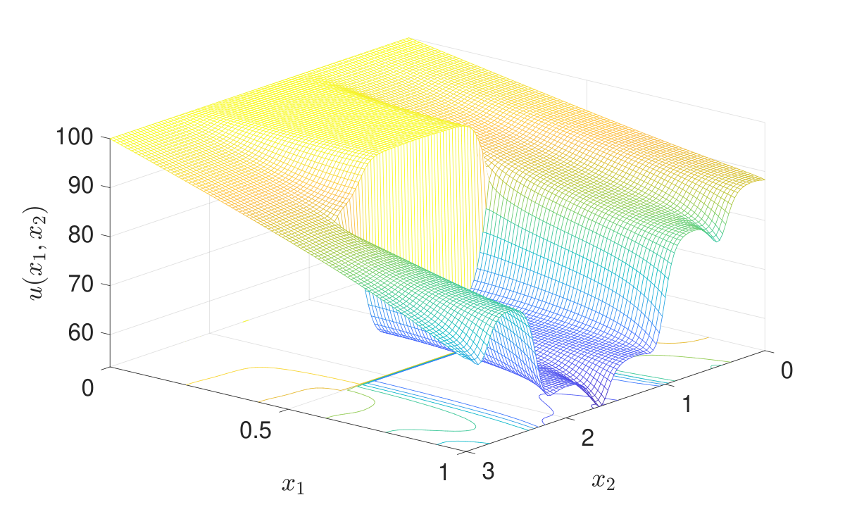
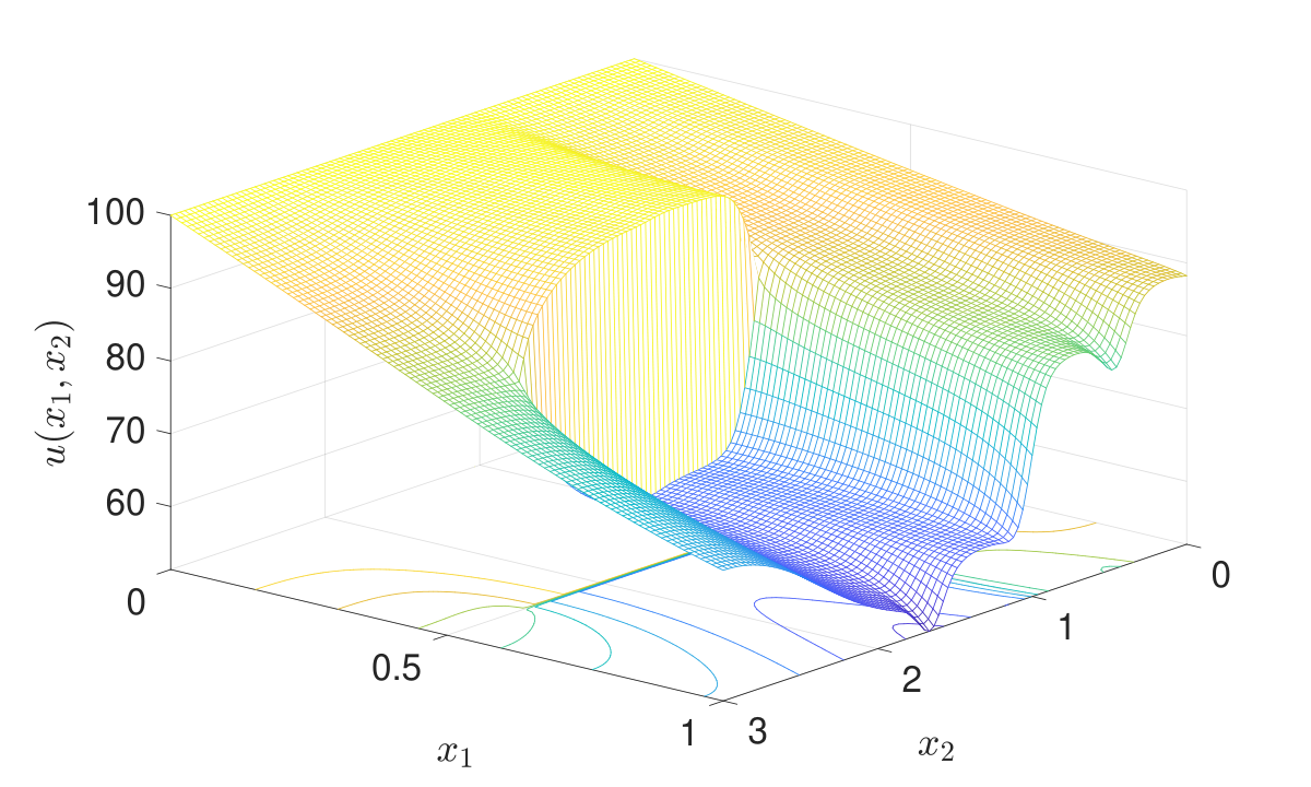
In Figures 8a and 8b, we present the prediction of the high fidelity model output for the proposed BTCK and the competitor.
We observe that BTCK managed to adequately capture the discontinuity and the smaller scale variations in the output while the competitor failed. We speculate that the behavior of the surface produced by the competitor in Figure 8b is because the basis expansion is unable to represent efficiently sudden changes. Moreover, the proposed BTCK produced a significantly smaller MSPE equal to compared to the competitor whose MSPE was . Hence the proposed BTCK has produced more accurate predictions than the competitor. Also, ABTCK managed to recover adequately the output function, even though the design was the same. Figures 9a and 9b demonstrate the estimation of the scale discrepancy function between models vs. and vs. respectively, as produced by the proposed ABTCK.

