Instance adaptive adversarial training:
Improved accuracy tradeoffs in neural nets
Abstract
Adversarial training is by far the most successful strategy for improving robustness of neural networks to adversarial attacks. Despite its success as a defense mechanism, adversarial training fails to generalize well to unperturbed test set. We hypothesize that this poor generalization is a consequence of adversarial training with uniform perturbation radius around every training sample. Samples close to decision boundary can be morphed into a different class under a small perturbation budget, and enforcing large margins around these samples produce poor decision boundaries that generalize poorly. Motivated by this hypothesis, we propose instance adaptive adversarial training – a technique that enforces sample-specific perturbation margins around every training sample. We show that using our approach, test accuracy on unperturbed samples improve with a marginal drop in robustness. Extensive experiments on CIFAR-10, CIFAR-100 and Imagenet datasets demonstrate the effectiveness of our proposed approach.
1 Introduction
A key challenge when deploying neural networks in safety-critical applications is their poor stability to input perturbations. Extremely tiny perturbations to network inputs may be imperceptible to the human eye, and yet cause major changes to outputs. One of the most effective and widely used methods for hardening networks to small perturbations is “adversarial training” (Madry et al. 2018), in which a network is trained using adversarially perturbed samples with a fixed perturbation size. By doing so, adversarial training typically tries to enforce that the output of a neural network remains nearly constant within an ball of every training input.
Despite its ability to increase robustness, adversarial training suffers from poor accuracy on clean (natural) test inputs. The drop in clean accuracy can be as high as on CIFAR-10, and on Imagenet (Madry et al. 2018; Xie et al. 2019), making robust models undesirable in some industrial settings. The consistently poor performance of robust models on clean data has lead to the line of thought that there may be a fundamental trade-off between robustness and accuracy (Zhang et al. 2019; Tsipras et al. 2019), and recent theoretical results characterized this tradeoff (Fawzi et al. 2018; Shafahi et al. 2018; Mahloujifar et al. 2019).
In this work, we aim to understand and optimize the tradeoff between robustness and clean accuracy. More concretely, our objective is to improve the clean accuracy of adversarial training for a chosen level of adversarial robustness. Our method is inspired by the observation that the constraints enforced by adversarial training are infeasible; for commonly used values of it is not possible to achieve label consistency within an -ball of each input image because the balls around images of different classes overlap. This is illustrated on the left of Figure 1, which shows that the -ball around a “bird” (from the CIFAR-10 training set) contains images of class “deer” (that do not appear in the training set). If adversarial training were successful at enforcing label stability in an ball around the “bird” training image, doing so would come at the unavoidable cost of misclassifying the nearby “deer” images that come along at test time. At the same time, when training images lie far from the decision boundary (eg., the deer image on the right in Fig 1), it is possible to enforce stability with large with no compromise in clean accuracy. When adversarial training on CIFAR-10, we see that is too large for some images, causing accuracy loss, while being unnecessarily small for others, leading to sub-optimal robustness.
The above observation naturally motivates adversarial training with instance adaptive perturbation radii that are customized to each training image. By choosing larger robustness radii at locations where class manifolds are far apart, and smaller radii at locations where class manifolds are close together, we get high adversarial robustness where possible while minimizing the clean accuracy loss that comes from enforcing overly-stringent constraints on images that lie near class boundaries. As a result, instance adaptive training significantly improves the tradeoff between accuracy and robustness, breaking through the pareto frontier achieved by standard adversarial training. Additionally, we show that the learned instance-specific perturbation radii are interpretable; samples with small radii are often ambiguous and have nearby images of another class, while images with large radii have unambiguous class labels that are difficult to manipulate.
Parallel to our work, we found that Ding et al. 2018 uses adaptive margins in a max-margin framework for adversarial training. Their work focuses on improving the adversarial robustness, which differs from our goal of understanding and improving the robustness-accuracy tradeoff. Moreover, our algorithm for choosing adaptive margins significantly differs from that of Ding et al. 2018.
2 Background
Adversarial attacks are data items containing small perturbations that cause misclassification in neural network classifiers (Szegedy et al. 2014). Popular methods for crafting attacks include the fast gradient sign method (FGSM) (Goodfellow et al. 2015) which is a one-step gradient attack, projected gradient descent (PGD) (Madry et al. 2018) which is a multi-step extension of FGSM, the C/W attack (Carlini & Wagner 2017), DeepFool (Moosavi-Dezfooli et al. 2016), and many more. All these methods use the gradient of the loss function with respect to inputs to construct additive perturbations with a norm-constraint. Alternative attack metrics include spatial transformer attacks (Xiao et al. 2018), attacks based on Wasserstein distance in pixel space (Wong et al. 2019), etc.
Defending against adversarial attacks is a crucial problem in machine learning. Many early defenses (Buckman et al. 2018; Samangouei et al. 2018; Dhillon et al. 2018), were broken by strong attacks. Fortunately, adversarially training is one defense strategy that remains fairly resistant to most existing attacks.
Let denote the set of training samples in the input dataset. In this paper, we focus on classification problems, hence, , where denotes the number of classes. Let denote a neural network model parameterized by . Classifiers are often trained by minimizing the cross entropy loss given by
where is the one-hot vector corresponding to the label . In adversarial training, instead of optimizing the neural network over the clean training set, we use the adversarially perturbed training set. Mathematically, this can be written as the following min-max problem
| (1) |
This problem is solved by an alternating stochastic method that takes minimization steps for followed by maximization steps that approximately solve the inner problem using steps of PGD. For more details, refer to Madry et al. 2018.
3 Instance Adaptive Adversarial Training
To remedy the shortcomings of uniform perturbation radius in adversarial training (Section 1), we propose Instance Adaptive Adversarial Training (IAAT), which solves the following optimization:
| (2) |
Like vanilla adversarial training, we solve this by sampling mini-batches of images , crafting adversarial perturbations of size at most , and then updating the network model using the perturbed images.
The proposed algorithm is distinctive in that it uses a different for each image Ideally, we would choose each to be as large as possible without finding images of a different class within the -ball around Since we have no a-priori knowledge of what this radius is, we use a simple heuristic to update after each epoch. After crafting a perturbation for we check if the perturbed image was a successful adversarial example. If PGD succeeded in finding an image with a different class label, then is too big, so we replace . If PGD failed, then we set .
Since the network is randomly initialized at the start of training, random predictions are made, and this causes to shrink rapidly. For this reason, we begin with a warmup period of a few (usually 10 epochs for CIFAR-10/100) epochs where adversarial training is performed using uniform for every sample. After the warmup period ends, we perform instance adaptive adversarial training.
A detailed training algorithm is provided in Alg. 1.
4 Experiments
To evaluate the robustness and generalization of our models, we report the following metrics: (1) test accuracy of unperturbed (natural) test samples, (2) adversarial accuracy of white-box PGD attacks, (3) adversarial accuracy of transfer attacks and (4) accuracy of test samples under common image corruptions (Hendrycks & Dietterich 2019). Following the protocol introduced in Hendrycks & Dietterich 2019, we do not train our models on any image corruptions.
4.1 CIFAR
On CIFAR-10 and CIFAR-100 datasets, we perform experiments on Resnet-18 and WideRenset-32-10 models following (Madry et al. 2018; Zhang et al. 2019). All models are trained on PGD- attacks i.e., steps of PGD iterations are used for crafting adversarial attacks during training. In the whitebox setting, models are evaluated on: (1) PGD- attacks with random restarts, (2) PGD- attacks with random restarts, and (3) PGD- attacks with random restarts. For transfer attacks, an independent copy of the model is trained using the same training algorithm and hyper-parameter settings, and PGD- adversarial attacks with random restarts are crafted on the surrogate model. For image corruptions, following (Hendrycks & Dietterich 2019), we report average classification accuracy on image corruptions.


Beating the robustness-accuracy tradeoff:
In adversarial training, the perturbation radius is a hyper-parameter. Training models with varying produces a robustness-accuracy tradeoff curve - models with small training achieve better natural accuracy and poor adversarial robustness, while models trained on large have improved robustness and poor natural accuracy. To generate this tradeoff, we perform adversarial training with in the range . Instance adaptive adversarial training is then compared with respect to this tradeoff curve in Fig. 3(a), 3(b). Two versions of IAAT are reported - with and without a warmup phase. In both versions, we clearly achieve an improvement over the accuracy-robustness tradeoff. Use of the warmup phase helps retain robustness with a drop in natural accuracy compared to its no-warmup counterpart.
Clean accuracy improves for a fixed level of robustness:
On CIFAR-10, as shown in Table. 1, we observe that our instance adaptive adversarial training algorithm achieves similar adversarial robustness as the adversarial training baseline. However, the accuracy on clean test samples increases by for Resnet-18 and for WideResnet-32-10. We also observe that the adaptive training algorithm improves robustness to unseen image corruptions. This points to an improvement in overall generalization ability of the network. On CIFAR-100 (Table. 2), the performance gain in natural test accuracy further increases - for Resnet-18, and for Wideresnet-32-10. The adversarial robustness drop is marginal.
| Method | Natural | Whitebox acc. (in ) | Transfer (in ) | Corruption | ||
| acc. (in ) | PGD10 | PGD100 | PGD1000 | acc. (PGD1000) | acc. (in ) | |
| Resnet-18 | ||||||
| Clean | 94.21 | 0.02 | 0.00 | 0.00 | 3.03 | 72.71 |
| Adversarial | 83.20 | 43.79 | 42.30 | 42.36 | 59.80 | 73.73 |
| IAAT | 87.26 | 43.08 | 41.16 | 41.16 | 59.87 | 78.82 |
| WideResnet 32-10 | ||||||
| Clean | 95.50 | 0.05 | 0.00 | 0.00 | 5.02 | 78.35 |
| Adversarial | 86.85 | 46.86 | 44.82 | 44.84 | 62.77 | 77.99 |
| IAAT | 91.34 | 48.53 | 46.50 | 46.54 | 58.20 | 83.13 |
| Method | Natural | Whitebox acc. (in ) | Transfer acc. (in ) | ||
| acc. (in ) | PGD10 | PGD100 | PGD1000 | PGD1000 | |
| Resnet-18 | |||||
| Clean | 74.88 | 0.02 | 0.00 | 0.01 | 1.81 |
| Adversarial | 55.11 | 20.69 | 19.68 | 19.91 | 35.57 |
| IAAT | 63.90 | 18.50 | 17.10 | 17.11 | 35.74 |
| WideResnet 32-10 | |||||
| Clean | 79.91 | 0.01 | 0.00 | 0.00 | 1.20 |
| Adversarial | 59.58 | 26.24 | 25.47 | 25.49 | 38.10 |
| IAAT | 68.80 | 26.17 | 24.22 | 24.36 | 35.18 |
Maintaining performance over a range of test :
Next, we plot adversarial robustness over a sweep of values used to craft attacks at test time. Fig. 4(a), 4(b) shows an adversarial training baseline with performs well at high regimes and poorly at low regimes. On the other hand, adversarial training with has a reverse effect, performing well at low and poorly at high regimes. Our instance adaptive training algorithm maintains good performance over all regimes, achieving slightly less performance than the model for small test and dominating all models for larger test


Interpretability of :
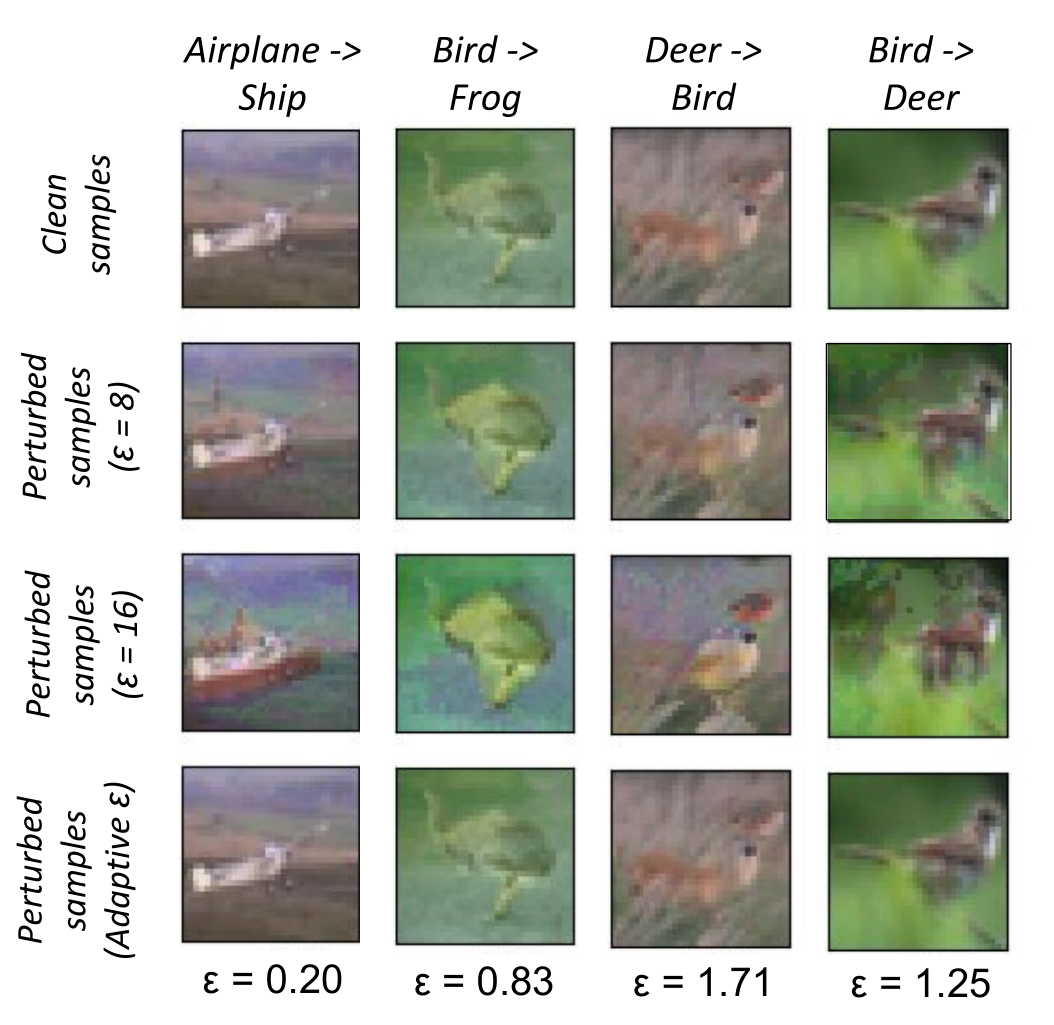
We find that the values of chosen by our adaptive algorithm correlate well with our own human concept of class ambiguity. Figure 2 (and Figure 7 in Appendix B) shows that a sampling of images that receive small contains many ambiguous images, and these images are perturbed into a (visually) different class using In contrast, images that receive a large have a visually definite class, and are not substantially altered by an perturbation.
4.2 Imagenet
Following the protocol introduced in Xie et al. 2019, we attack Imagenet models using random targeted attacks instead of untargeted attacks as done in previous experiments. During training, adversarial attacks are generated using steps of PGD. As a baseline, we use adversarial training with a fixed of . This is the setting used in Xie et al. 2019. Adversarial training on Imagenet is computationally intensive. To make training practical, we use distributed training with synchronized SGD on GPUs. More implementation details can be found in Appendix D.
At test time, we evaluate the models on clean test samples and on whitebox adversarial attacks with . PGD- attacks are used. Additionally, we also report normalized mean corruption error (mCE), an evaluation metric introduced in Hendrycks & Dietterich 2019 to test the robustness of neural networks to image corruptions. This metric reports mean classification error of different image corruptions averaged over varying levels of degradation. Note that while accuracies are reported for natural and adversarial robustness, mCE reports classification errors, so lower numbers are better.
Our experimental results are reported in Table. 3. We observe a huge drop in natural accuracy for adversarial training (, and drop for Resnet-50, 101 and 152 respectively). Adaptive adversarial training significantly improves the natural accuracy - we obtain a consistent performance gain of on all three models over the adversarial training baseline. On whitebox attacks, IAAT outperforms the adversarial training baseline on low regimes, however a drop of is observed at high ’s (). On the corruption dataset, our model consistently outperforms adversarial training.
| Method | Natural | Whitebox acc. (in ) () | Corruption | |||
| acc. (in ) () | mCE () | |||||
| Resnet-50 | ||||||
| Clean training | 75.80 | 0.64 | 0.18 | 0.00 | 0.00 | 76.69 |
| Adversarial training | 50.99 | 50.89 | 49.11 | 44.71 | 35.82 | 95.48 |
| IAAT | 62.71 | 61.52 | 54.63 | 39.90 | 22.72 | 85.21 |
| Resnet-101 | ||||||
| Clean training | 77.10 | 0.83 | 0.12 | 0.00 | 0.00 | 70.37 |
| Adversarial training | 55.42 | 55.11 | 53.07 | 48.35 | 39.08 | 91.45 |
| IAAT | 65.29 | 63.83 | 56.62 | 41.51 | 23.91 | 79.52 |
| Resnet-152 | ||||||
| Clean training | 77.60 | 0.57 | 0.08 | 0.00 | 0.00 | 69.27 |
| Adversarial training | 57.26 | 56.77 | 54.75 | 49.86 | 40.40 | 89.31 |
| IAAT | 67.44 | 65.97 | 59.28 | 45.01 | 27.85 | 78.53 |
5 Ablation experiments
5.1 Effect of warmup
| Method | Natural | Whitebox acc. (in ) | Transfer acc.() | Corruption | ||
| acc. () | PGD10 | PGD100 | PGD1000 | PGD1000 | acc. (in ) | |
| Resnet-18 | ||||||
| IAAT (no warm) | 89.62 | 40.55 | 38.15 | 38.08 | 58.89 | 81.10 |
| IAAT (warm) | 87.26 | 43.08 | 41.16 | 41.16 | 59.87 | 78.82 |
| WideResnet 32-10 | ||||||
| IAAT (no warm) | 92.62 | 45.12 | 41.08 | 41.11 | 53.08 | 84.92 |
| IAAT (warm) | 90.67 | 48.53 | 46.50 | 46.54 | 58.20 | 83.13 |
| Method | Natural | Whitebox acc. (in ) | Transfer acc.() | ||
| acc. (in ) | PGD10 | PGD100 | PGD1000 | PGD1000 | |
| Resnet-18 | |||||
| Adaptive (no warm) | 68.34 | 14.76 | 13.29 | 13.30 | 32.39 |
| Adaptive (warm) | 63.90 | 18.50 | 17.10 | 17.11 | 35.74 |
| WideResnet 32-10 | |||||
| Adaptive (no warm) | 75.48 | 18.14 | 13.78 | 13.71 | 24.00 |
| Adaptive (warm) | 68.80 | 26.17 | 24.22 | 24.36 | 35.18 |
In this section, we study the effect of using a warmup phase in adaptive adversarial training. Recall from Section 3 that during warmup, adversarial training is performed with uniform norm-bound constraints. Once the warmup phase ends, we switch to instance adaptive training. From Table 4 and 5, we observe that when warmup is used, adversarial robustness improves with a small drop in natural accuracy. The improvement in robustness is more pronounced in the CIFAR-100 dataset. However, as shown in Fig. 3(a) and 3(b), both these settings improve the accuracy-robustness tradeoff.


5.2 Visualizing progress
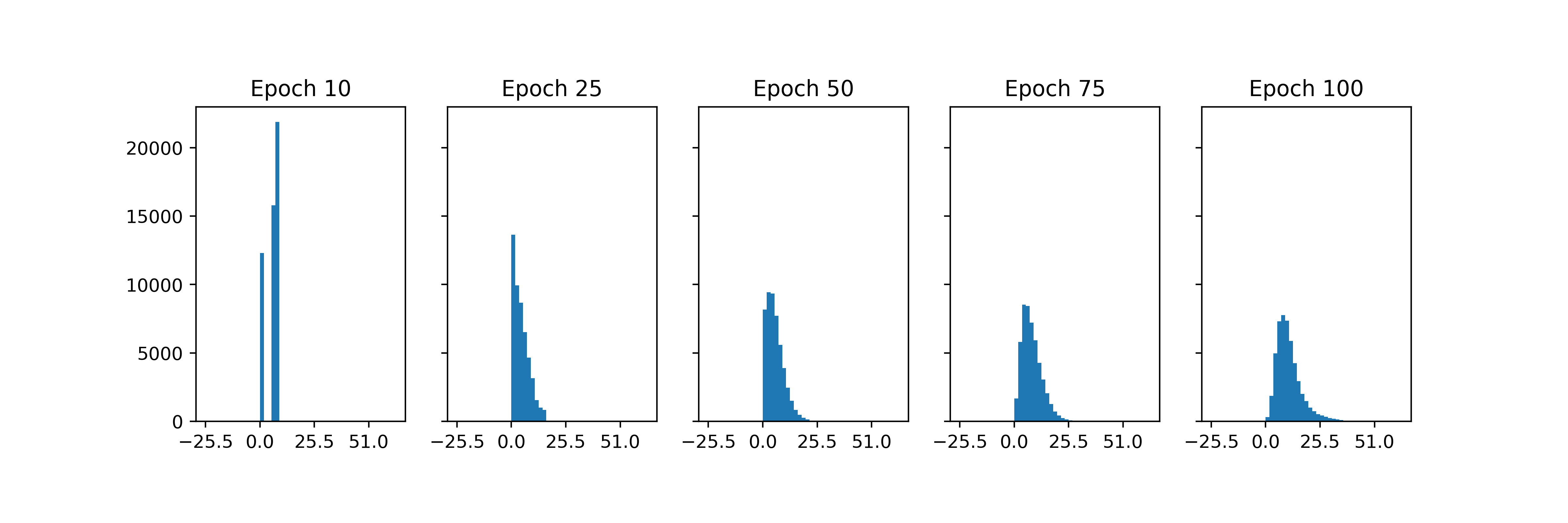
Next, we visualize the evolution of over epochs in adaptive adversarial training. A plot showing the average growth, along with the progress of randomly picked samples are shown in Fig. 5(a) and 5(b). We observe that average converges to around , which is higher than the default setting of used in adversarial training. Also, each sample has a different profile - for some, increases well beyond the commonly use radius of , while for others, it converges below it. In addition, a plot showing the histogram of ’s at different snapshots of training is shown in Fig. 8. We observe an increase in spread of the histogram as the training progresses.
6 Conclusion
In this work, we focus on improving the robustness-accuracy tradeoff in adversarial training. We first show that realizable robustness is a sample-specific attribute: samples close to the decision boundary can only achieve robustness within a small ball, as they contain samples from a different class beyond this radius. On the other hand samples far from the decision boundary can be robust on a relatively large perturbation radius. Motivated by this observation, we develop instance adaptive adversarial training, in which label consistency constraints are imposed within sample-specific perturbation radii, which are in-turn estimated. Our proposed algorithm has empirically been shown to improve the robustness-accuracy tradeoff in CIFAR-10, CIFAR-100 and Imagenet datasets.
7 Acknowledgements
Goldstein and Balaji were supported in part by the DARPA GARD program, DARPA QED for RML, DARPA Lifelong Learning Machines, the DARPA Young Faculty Award program, the AFOSR MURI program, and the National Science Foundation.
References
- Buckman et al. (2018) Jacob Buckman, Aurko Roy, Colin Raffel, and Ian Goodfellow. Thermometer encoding: One hot way to resist adversarial examples. In International Conference on Learning Representations, 2018. URL https://openreview.net/forum?id=S18Su--CW.
- Carlini & Wagner (2017) Nicholas Carlini and David A. Wagner. Towards evaluating the robustness of neural networks. In 2017 IEEE Symposium on Security and Privacy, SP 2017, San Jose, CA, USA, May 22-26, 2017, pp. 39–57, 2017.
- Dhillon et al. (2018) Guneet S. Dhillon, Kamyar Azizzadenesheli, Jeremy D. Bernstein, Jean Kossaifi, Aran Khanna, Zachary C. Lipton, and Animashree Anandkumar. Stochastic activation pruning for robust adversarial defense. In International Conference on Learning Representations, 2018. URL https://openreview.net/forum?id=H1uR4GZRZ.
- Ding et al. (2018) Gavin Weiguang Ding, Yash Sharma, Kry Yik Chau Lui, and Ruitong Huang. Max-margin adversarial (mma) training: Direct input space margin maximization through adversarial training. arXiv preprint arXiv:1812.02637, 2018.
- Fawzi et al. (2018) Alhussein Fawzi, Hamza Fawzi, and Omar Fawzi. Adversarial vulnerability for any classifier. In Advances in Neural Information Processing Systems, pp. 1178–1187, 2018.
- Goodfellow et al. (2015) Ian J. Goodfellow, Jonathon Shlens, and Christian Szegedy. Explaining and harnessing adversarial examples. In 3rd International Conference on Learning Representations, ICLR 2015, San Diego, CA, USA, May 7-9, 2015, Conference Track Proceedings, 2015. URL http://arxiv.org/abs/1412.6572.
- Goyal et al. (2017) Priya Goyal, Piotr Dollár, Ross Girshick, Pieter Noordhuis, Lukasz Wesolowski, Aapo Kyrola, Andrew Tulloch, Yangqing Jia, and Kaiming He. Accurate, large minibatch sgd: Training imagenet in 1 hour. arXiv preprint arXiv:1706.02677, 2017.
- Hendrycks & Dietterich (2019) Dan Hendrycks and Thomas Dietterich. Benchmarking neural network robustness to common corruptions and perturbations. In International Conference on Learning Representations, 2019. URL https://openreview.net/forum?id=HJz6tiCqYm.
- Lamb et al. (2019) Alex Lamb, Vikas Verma, Juho Kannala, and Yoshua Bengio. Interpolated adversarial training: Achieving robust neural networks without sacrificing accuracy. CoRR, abs/1906.06784, 2019.
- Madry et al. (2018) Aleksander Madry, Aleksandar Makelov, Ludwig Schmidt, Dimitris Tsipras, and Adrian Vladu. Towards deep learning models resistant to adversarial attacks. In International Conference on Learning Representations, 2018. URL https://openreview.net/forum?id=rJzIBfZAb.
- Mahloujifar et al. (2019) Saeed Mahloujifar, Dimitrios I Diochnos, and Mohammad Mahmoody. The curse of concentration in robust learning: Evasion and poisoning attacks from concentration of measure. In Proceedings of the AAAI Conference on Artificial Intelligence, volume 33, pp. 4536–4543, 2019.
- Moosavi-Dezfooli et al. (2016) Seyed-Mohsen Moosavi-Dezfooli, Alhussein Fawzi, and Pascal Frossard. Deepfool: A simple and accurate method to fool deep neural networks. In 2016 IEEE Conference on Computer Vision and Pattern Recognition, CVPR 2016, Las Vegas, NV, USA, June 27-30, 2016, pp. 2574–2582, 2016.
- Samangouei et al. (2018) Pouya Samangouei, Maya Kabkab, and Rama Chellappa. Defense-GAN: Protecting classifiers against adversarial attacks using generative models. In International Conference on Learning Representations, 2018. URL https://openreview.net/forum?id=BkJ3ibb0-.
- Shafahi et al. (2018) Ali Shafahi, W Ronny Huang, Christoph Studer, Soheil Feizi, and Tom Goldstein. Are adversarial examples inevitable? arXiv preprint arXiv:1809.02104, 2018.
- Szegedy et al. (2014) Christian Szegedy, Wojciech Zaremba, Ilya Sutskever, Joan Bruna, Dumitru Erhan, Ian Goodfellow, and Rob Fergus. Intriguing properties of neural networks. In International Conference on Learning Representations, 2014. URL http://arxiv.org/abs/1312.6199.
- Tsipras et al. (2019) Dimitris Tsipras, Shibani Santurkar, Logan Engstrom, Alexander Turner, and Aleksander Madry. Robustness may be at odds with accuracy. In 7th International Conference on Learning Representations, ICLR 2019, New Orleans, LA, USA, May 6-9, 2019, 2019.
- Wong et al. (2019) Eric Wong, Frank Schmidt, and Zico Kolter. Wasserstein adversarial examples via projected Sinkhorn iterations. In Kamalika Chaudhuri and Ruslan Salakhutdinov (eds.), Proceedings of the 36th International Conference on Machine Learning, Proceedings of Machine Learning Research, pp. 6808–6817. PMLR, 2019.
- Xiao et al. (2018) Chaowei Xiao, Jun-Yan Zhu, Bo Li, Warren He, Mingyan Liu, and Dawn Song. Spatially transformed adversarial examples. In International Conference on Learning Representations, 2018. URL https://openreview.net/forum?id=HyydRMZC-.
- Xie et al. (2019) Cihang Xie, Yuxin Wu, Laurens van der Maaten, Alan L. Yuille, and Kaiming He. Feature denoising for improving adversarial robustness. In The IEEE Conference on Computer Vision and Pattern Recognition (CVPR), June 2019.
- Zhang et al. (2019) Hongyang Zhang, Yaodong Yu, Jiantao Jiao, Eric Xing, Laurent El Ghaoui, and Michael Jordan. Theoretically principled trade-off between robustness and accuracy. In Kamalika Chaudhuri and Ruslan Salakhutdinov (eds.), Proceedings of the 36th International Conference on Machine Learning, volume 97 of Proceedings of Machine Learning Research, pp. 7472–7482, Long Beach, California, USA, 09–15 Jun 2019. PMLR. URL http://proceedings.mlr.press/v97/zhang19p.html.
Appendix A Appendix
A.1 Comparison with Mixup
A recent paper that addresses the problem of improving natural accuracy in adversarial training is mixup adversarial training (Lamb et al. 2019), where adversarially trained models are optimized using mixup loss instead of the standard cross-entropy loss. In this paper, natural accuracy was shown to improve with no drop in adversarial robustness. However, the robustness experiments were not evaluated on strong attacks (experiments were reported only on PGD-20). We compare our implementation of mixup adversarial training with IAAT on stronger attacks in Table. 6. We observe that while natural accuracy improves for mixup, drop in adversarial accuracy is much higher than IAAT.
| Method | Natural | Whitebox acc. (in ) | Transfer attack (in ) | ||
| acc. (in ) | PGD10 | PGD100 | PGD1000 | PGD1000 | |
| Resnet-18 | |||||
| Mixup | 89.47 | 42.60 | 38.42 | 38.49 | 59.48 |
| IAAT | 87.26 | 43.08 | 41.16 | 41.16 | 59.87 |
| WideResnet 32-10 | |||||
| Mixup | 92.57 | 45.01 | 36.6 | 36.44 | 63.57 |
| IAAT | 90.67 | 48.53 | 46.50 | 46.54 | 58.20 |
Appendix B Sample visualization
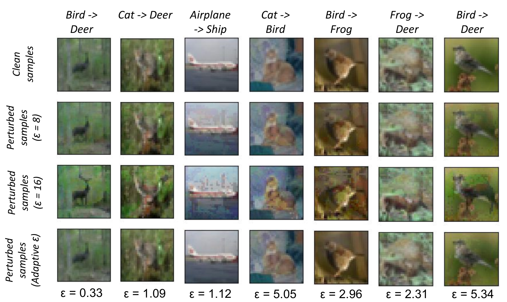
A visualization of samples from CIFAR-10 dataset with the corresponding value assigned by IAAT is shown in Figure. 6. We observe that samples for which low ’s are assigned are visually confusing (eg., top row of Figure. 6), while samples with high distinctively belong to one class.

In addition, we also show more visualizations of samples near decision boundary which contain samples from a different class within a fixed ball in Figure. 7. The infeasibility of label consistency constraints within the commonly used perturbation radius of is apparent in this visualization. Our algorithm effectively chooses an appropriate that retains label information within the chosen radius.
Appendix C Imagenet sweep over PGD iterations
Testing against a strong adversary is crucial to assess the true robustness of a model. A popular practice in adversarial robustness community is to attack models using PGD with many attack iterations (Xie et al. 2019). So, we test our instance adaptive adversarially trained models on a sweep of PGD iterations for a fixed level. Following (Xie et al. 2019), we perform the sweep upto attack steps fixing . The resulting plot is shown in Figure. 9. For all three Resnet models, we observe a saturation in adversarial robustness beyond 500 attack iterations.
Appendix D Implementation details
D.1 CIFAR
On CIFAR-10 and CIFAR-100 datasets, our implementation follows the standard adversarial training setting used in Madry et al. 2018. During training, adversarial examples are generated using PGD-10 attacks, which are then used to update the model. All hyperparameters we used are tabulated in Table. 7.
| Hyperparameters | Resnet-18 | WideResnet-32-10 |
|---|---|---|
| Optimizer | SGD | SGD |
| Start learning rate | 0.1 | 0.1 |
| Weight decay | 0.0002 | 0.0005 |
| Number of epochs trained | 200 | 110 |
| Learning rate annealing | Step decay | Step decay |
| Learning rate decay steps | [80, 140, 170] | [70, 90, 100] |
| Learning rate decay factor | 0.1 | 0.2 |
| Batch size | 128 | 128 |
| Warmup period | 5 epochs | 10 epochs |
| used in warmup () | 8 | 8 |
| Discretization | 1.9 | 1.9 |
| Exponential averaging factor | 0.1 | 0.1 |
| Attack parameters during training | ||
| Attack steps | 10 | 10 |
| Attack (for adv. training only) | 8 | 8 |
| Attack learning rate | 2/255 | 2/255 |
D.2 Imagenet
For Imagenet implementation, we mimic the setting used in Xie et al. 2019. During training, adversaries are generated with PGD-30 attacks. This is computationally expensive as every training update is followed by backprop iterations to generate the adversarial attack. To make training feasible, we perform distributed training using synchronized SGD updates on 64 / 128 GPUs. We follow the training recipe introduced in Goyal et al. 2017 for large batch training. Also, during training, adversarial attacks are generated with FP-16 precision. However, in test phase, we use FP-32.
We further use two more tricks to speed-up instance adaptive adversarial training: (1) A weaker attacker(PGD-10) is used in the algorithm for selecting (Alg. 2). (2) After is selected per Alg. 2, we clip it with a lower-bound i.e., . was used in our experiments.
Hyperparameters used in our experiments are reported in Table 8. All our models were trained on PyTorch.
| Hyperparameters | Imagenet |
|---|---|
| Optimizer | SGD |
| Start learning rate | 0.1 (effective batch size / 256) |
| Weight decay | 0.0001 |
| Number of epochs trained | 110 |
| Learning rate annealing | Step decay with LR warmup |
| Learning rate decay steps | [35, 70, 95] |
| Learning rate decay factor | 0.1 |
| Batch size | 32 per GPU |
| Warmup period | 30 epochs |
| used in warmup () | 16 |
| Discretization | 4 |
| Exponential averaging factor | 0.1 |
| Attack parameters during training | |
| Attack steps | 30 |
| Attack (for adv. training only) | 16 |
| Attack learning rate | 1/255 |
Resnet-50 model was trained on 64 Nvidia V100 GPUs, while Resnet-101 and Resnet-152 models were trained on 128 GPUs. Time taken for instance adaptive adversarial training for all models is reported in Table. 9.
| Model | Number of GPUs used | Training time |
|---|---|---|
| Resnet-50 | 64 | 92 hrs |
| Resnet-101 | 128 | 78 hrs |
| Resnet-152 | 128 | 94 hrs |