Bayes Linear Emulation of Simulator Networks

Samuel E. Jackson Note: samuel.e.jackson@ucl.ac.uk Affiliation: Clinical Operations Research Unit, University College London, London, UK Affiliation: David C. Woods Affiliation: Southampton Statistical Sciences Research Institute, University of Southampton, Affiliation: Southampton, UK

Abstract

Computationally expensive simulators, implementing mathematical models in computer codes, are commonly approximated using statistical emulators. We develop and assess novel emulation methods for systems best modelled via a chain, series or network of simulators. Using a Bayes linear framework, we link statistical emulators of the component simulators to explicitly account for the simulator input uncertainty induced by links between models in arbitrarily large networks. We demonstrate the advantages of these methods compared to use of a single emulator of the composite simulator network for a variety of examples, including the motivating epidemiological simulator chain to model the impact of an airborne infectious disease.

1 Introduction

Scientific processes are commonly modelled using mathematical models implemented in computer codes, or simulators, that encapsulate the key features of the system and facilitate prediction and decision making. Complex systems can often be most appropriately modelled as a network of simpler component simulators, that together form a composite simulator of the entire system of interest. In this paper, we develop statistical emulation methods to facilitate uncertainty quantification for such simulator networks.

One simple, but important, example from epidemiology combines an atmospheric Anthrax dispersion simulator (Legrand et al. 2009), labelled $d(\cdot)$ , with a dose-response (DR) simulator (Groer 1978), labelled $\rho(\cdot)$ , in a simple chain network; see Figure 1. The composite dispersion dose-response (DDR) simulator $h=\rho(d(\mathbf{z}))$ models the overall process, where $\mathbf{z}$ can be viewed as the input to $d$ or $h$ .

In the specific application we consider, the dispersion simulator models the spread of a released biological agent across a given spatial domain, with input parameters of interest corresponding to physical quantities wind speed ( $z_{WS}$ ), wind direction ( $z_{WD}$ ) and source mass ( $z_{SM}$ ). Simulator outputs $d(\mathbf{z})$ represent dose at each location across the domain.

For a given spatial location, the DR simulator takes dose, $x$ , as input and outputs casualties, $\rho(x)$ , as a proportion of the population at that location. When combined into a modelling chain, we take $x=d(\mathbf{z})$ . That is, the output from the dispersion simulator becomes the input to the DR simulator.

Figure 1: Graphical representation of the DDR network of simulators

h(\mathbf{z})=\rho(d(\mathbf{z}))

The primary interest of decision makers is the impact of release conditions on numbers of casualties. This assessment requires linking the two component simulators, each of which implements modelling from two different groups of experts. Other applications involving chained simulators include modelling of climate (Taylor et al. 2012) and seismic activity (Jha & Juanes 2014).

Utilising simulator networks for uncertainty quantification is challenging, largely due to the variety of sources of uncertainty for each individual component simulator (Goldstein et al. 2013) and the necessity of propagating that uncertainty through the network. In particular, the computational expense of a typical simulator leads to substantial output uncertainty across the input space due to the small number of input combinations for which it is feasible to run the simulator. Often, this uncertainty is captured by building a statistical approximation, or emulator, of the simulator using a computer experiment. In this paper, we answer the important, yet rather under-explored, question of whether combining emulators for the component simulators within a network can result in more powerful approximations than emulating the network as a single composite simulator. In particular, we present two novel approaches for linking Bayes linear emulators, which extend to arbitrarily large networks of simulators, as well as overcoming certain limitations on the structural form of the emulators seen in related work (for example Kyzyurova et al. 2018 and Section 2).

The article is outlined as follows. We formally introduce concepts, notation and previous work for simulator networks in Section 2. In Section 3, we present the two novel approaches alluded to above, before demonstrating their efficacy in Section 4, using the epidemiological application, by comparison to direct emulation of the composite simulator. Motivated by this application, much of the article focuses on the relatively simple composite simulator formed of two component simulators, however, in Section 5 we demonstrate the methodology on a more complicated network of simulators. Section 6 contains a brief discussion and some directions for future research. The methods in this paper are implemented in the R package NetworkPPBLE available at https://github.com/Jackson-SE/NetworkPPBLE.

2 Networks of Simulators

We represent a simulator network as a directed acyclic graph (Thulasiraman & Swamy 1992, DAG;) with nodes $\mathbf{f}^{0},\dots,\mathbf{f}^{w}$ :

1.

$\mathbf{f}^{0}=\mathbf{z}$ is a root note (in-degree of zero), representing a $p_{z}$ -vector of independent inputs, where $\mathbf{z}\in\mathbb{Z}\subseteq\mathbb{R}^{p_{z}}$ and
2.

$\mathbf{f}^{i}=\mathbf{f}^{i}(\cdot),i=1,\dots,w,$ represent component simulators with generic $p_{i}$ -vector inputs $\mathbf{x}_{i}\in\mathbb{X}_{i}\subseteq\mathbb{R}^{p_{i}}$ and $q_{i}$ -vector outputs.

The edges of the DAG represent directed links between simulators; there is an edge from node $\mathbf{f}^{i}$ to $\mathbf{f}^{j}$ if an output from simulator $\mathbf{f}^{i}$ is an input to simulator $\mathbf{f}^{j}$ . Further, we order the nodes such that a directed edge can only exist from $\mathbf{f}^{i}$ to $\mathbf{f}^{j}$ if $i<j$ ( $i,j=1,\dots,w$ ).

In general, we can now consider methods of emulating $\mathbf{f}^{j}$ , given that there is at least one occasion where $x_{j(r)}=f^{i}_{k}(\mathbf{x}_{i})$ , that is, where the $r$ th input to the $j$ th simulator arises as the $k$ th output from the $i$ th simulator, $i<j$ . For any such inputs, note that we also require $f_{k}(\mathbb{X}_{i})\subseteq\mathbb{X}_{j(r)}$ , where $\mathbb{X}_{j(r)}$ is the domain for the $r$ th input to the $j$ th simulator and $f_{k}(\mathbb{X}_{i})$ is the domain for the $k$ th output of the $i$ th simulator. For well designed simulator networks, this restriction will be satisfied automatically.

Figure 2: DAGs representing; left: a simple chain network of two simulators, and right: a more complex network of simulators.

Figure 2 shows two DAGs representing simulator networks. The left-hand DAG represents a simple chain network of two simulators, which, for clarity, we take as the main focus of the article. Such a chain may represent the simple network example of Section 2.3, the example of Kyzyurova et al. 2018 (discussed below), or the DDR example introduced in Section 1 and explored in Section 4. The right-hand DAG shows a more complex network of simulators, as is used in Section 5 to demonstrate the generality of our methods.

When one or more of the individual simulators $\mathbf{f}^{i}$ , $i<w$ , is computationally expensive and requires the construction of an emulator, the uncertainty arising from the emulation must be propagated through the network. We focus on linking Bayes linear emulators for each component simulator and compare to the direct construction of a single emulator for the composite simulator. Essentially, this results in the requirement to build emulators where one or more simulator inputs are uncertain in the computer experiment.

In previous related work, Kyzyurova et al. 2018 proposed coupling two simulators by linking independently developed Gaussian process (GP) emulators of the simulators. Their motivation arose from potentially having separate training runs for two simulators $\mathbf{f}^{1}=$ bent and $\mathbf{f}^{2}=$ puff, where bent simulates volcanic ash plumes arising from a vent and puff simulates ash dispersion. As a result, direct emulation (see Section 2.2) of the composite simulator defined by the chain is not possible. For specific GP forms, they derived closed form expressions for the overall mean and variance arising from linking the two emulators and applied these quantities within a normal distribution approximation for the composite emulator. This availability of second-order posterior statistics for the chain, but the lack of a closed-form distribution, has inspired us to investigate (Bayes linear) approaches to emulation in this context (see Section 2.1). In addition, these Bayes linear approaches remove the requirements that the inputs $\mathbf{x}_{j}$ to $\mathbf{f}^{j}$ must follow a particular distributional form, and that the correlation functions for each component emulator must be power exponential in form, as well as naturally extending to arbitrarily larger networks.

More broadly, literature exists concerning the problem of training emulators of simulators with inputs perturbed by noise, often assuming that the magnitude of the noise is uncertain and typically modelled using one or more additional hyperparameters. For example, McHutchon & Rasmussen 2011 made use of local linear expansions about each input point to allow input noise to be recast as output noise that is proportional to the squared gradient of the GP posterior mean. Under our definition of a simulator network, input uncertainty at a given input is assumed to be represented in the form of a second-order belief specification (arising from the posterior beliefs of a previous emulator).

Emulating simulator networks can also be compared to emulation using deep GPs (Damianou & Lawrence 2013; Dunlop et al. 2018). Deep GPs arise from belief networks about simulator behaviour based on GP mappings, such that layers of GP latent variables exist between simulator input and output, these being marginalised variationally (see, for example, Titisias & Lawrence 2010). Whilst similar, the intermediate variables in a simulator network represent physical system properties, which aids the construction and modelling of the emulators for each of the component processes. Direct use of a deep GP for the entire network will not exploit this additional information. However, such ideas may be applicable to aid emulation of the component simulators, which can then be linked together using the methods that we present here.

Bayes Linear Emulation

In this section we review general Bayes linear emulation methodology, using notation for a generic simulator $\mathbf{f}$ . The simulator has input vector $\mathbf{x}=(x_{(1)},\dots,x_{(p)})\in\mathbb{X}\subseteq\mathbb{R}^{p}$ , and outputs vector $\mathbf{f}(\mathbf{x})=(f_{1}(\mathbf{x}),\dots,f_{q}(\mathbf{x}))\in\mathbf{f}(\mathbb{X})\subseteq\mathbb{R}^{q}$ . We represent our beliefs about the behaviour of $\mathbf{f}(\mathbf{x})$ in the following form (Goldstein & Rougier 2004):

\mathbf{f}(\mathbf{x})=\mathbf{g}(\mathbf{x})^{T}\bm{B}+\mathbf{u}(\mathbf{x})\,,

(1)

where $\mathbf{g}(\mathbf{x})$ is an $m$ -vector of known basis regression functions, $\bm{B}$ is an $m\times q$ matrix of unknown regression coefficients, and $\mathbf{u}(\mathbf{x})$ is a $q$ -dimensional weakly-stationary stochastic process.

Let $\bm{\beta}=\textrm{vec}{(\bm{B})}$ be an $mq$ -vector resulting from stacking the columns of $\bm{B}$ , with a generic prior specification ${\rm E}[\bm{\beta}]=\bm{\Gamma}$ and ${\rm Var}[\bm{\beta}]=\bm{\mathit{\Delta}}$ . We also make the common assumptions that ${\rm E}[\mathbf{u}(\mathbf{x})]=\mathbf{0}$ , ${\rm Cov}\left[\bm{\beta},\mathbf{u}(\mathbf{x})\right]=\bm{\mathit{0}}$ , and covariance between $\mathbf{u}(\mathbf{x})$ and $\mathbf{u}(\mathbf{x}^{\prime})$ is of the form

\textrm{Cov}[\mathbf{u}(\mathbf{x}),\mathbf{u}(\mathbf{x}^{\prime})]=c(\mathbf{x},\mathbf{x}^{\prime})\,\bm{\mathit{\Sigma}}\,,

(2)

for two inputs $\mathbf{x}$ and $\mathbf{x}^{\prime}$ . Here, $\bm{\mathit{\Sigma}}$ is a $q\times q$ output covariance matrix and $c(\mathbf{x},\mathbf{x}^{\prime})$ is a stationary correlation function of $\mathbf{x}$ and $\mathbf{x}^{\prime}$ (Koehler & Owen 1996; Kennedy & O’Hagan 2001); for example, the Gaussian correlation function

c(\mathbf{x},\mathbf{x}^{\prime})=\exp\left\{-\sum_{r=1}^{p}\left(\frac{x_{(r)}-x^{\prime}_{(r)}}{\theta_{r}}\right)^{2}\right\},

(3)

which depends on the specification of the correlation length parameters $\theta_{r},r=1,...,p$ .

Suppose $\mathbf{F}=\mathbf{f}(\mathcal{X})=(\mathbf{f}_{1}(\mathcal{X})^{T},\dots,\mathbf{f}_{q}(\mathcal{X})^{T})^{T}$ is an $nq$ -vector with $\mathbf{f}_{k}(\mathcal{X})$ being $n$ -vectors of simulator output $k=1,\dots,q$ run at each row of the $n\times p$ design matrix $\mathcal{X}=(\mathbf{x}^{(1)},\dots,\mathbf{x}^{(n)})^{T}$ . We can adjust our second-order prior belief specification about $\mathbf{f}(\mathbf{x})$ across $\mathcal{X}$ by $\mathbf{F}$ using the Bayes linear update equations to obtain posterior quantities:

{\rm E}_{\mathbf{F}}[\mathbf{f}(\mathbf{x})]={\rm E}[\mathbf{f}(\mathbf{x})]+{\rm Cov}\left[\mathbf{f}(\mathbf{x}),\mathbf{F}\right]{\rm Var}[\mathbf{F}]^{-1}(\mathbf{F}-{\rm E}[\mathbf{F}])

(4)

{\rm Var}_{\mathbf{F}}[\mathbf{f}(\mathbf{x})]={\rm Var}[\mathbf{f}(\mathbf{x})]-{\rm Cov}\left[\mathbf{f}(\mathbf{x}),\mathbf{F}\right]{\rm Var}[\mathbf{F}]^{-1}{\rm Cov}\left[\mathbf{F},\mathbf{f}(\mathbf{x})\right]\,.

(5)

See the supplementary material for further details of the Bayes linear approach.

It is worth noting that avoiding unnecessary distributional assumptions is a general advantage of the Bayes linear approach to statistical inference. Inferential statements can still be made, using results such as Chebyshev’s inequality (Chebyshev 1867) or Pukelsheim’s $3\sigma$ rule (Pukelsheim 1994).

Direct Emulation of Simulator Network (DE)

Let $\mathbf{h}$ represent a simulator network, so that $\mathbf{h}(\mathbf{z})$ denotes running the resulting composite simulator starting with initial inputs $\mathbf{z}$ . The aim throughout this article is to develop appropriate mean and variance estimators, $\bm{\mu}_{\mathbf{h}}(\mathbf{z})$ and $\bm{\nu}_{\mathbf{h}}(\mathbf{z})$ , for $\mathbf{h}(\mathbf{z})$ .

An obvious estimation approach is Direct Emulation (DE) of $\mathbf{h}$ , which involves applying the Bayes linear update Equations (4) and (5) directly to $\mathbf{h}$ :

	$\displaystyle\bm{\mu}_{\mathbf{h}}(\mathbf{z})$	$\displaystyle\,=$	$\displaystyle\,{\rm E}_{\mathbf{H}}[\mathbf{h}(\mathbf{z})]\,\,$	$\displaystyle\,=$		$\displaystyle\,\,{\rm E}[\mathbf{h}(\mathbf{z})]+{\rm Cov}\left[\mathbf{h}(\mathbf{z}),\mathbf{H}\right]{\rm Var}[\mathbf{H}]^{-1}(\mathbf{H}-{\rm E}[\mathbf{H}])$		(6)
	$\displaystyle\bm{\nu}_{\mathbf{h}}(\mathbf{z})$	$\displaystyle\,=$	$\displaystyle\,{\rm Var}_{\mathbf{H}}[\mathbf{h}(\mathbf{z})]$	$\displaystyle\,=$		$\displaystyle\,\,\textrm{Var}[\mathbf{h}(\mathbf{z})]-{\rm Cov}\left[\mathbf{h}(\mathbf{z}),\mathbf{H}\right]{\rm Var}[\mathbf{H}]^{-1}{\rm Cov}\left[\mathbf{H},\mathbf{h}(\mathbf{z})\right],$		(7)

with $\mathbf{H}=\mathbf{h}(\mathcal{Z})$ being $n_{z}$ training runs at input locations given by the $n_{z}\times p_{z}$ design matrix $\mathcal{Z}$ . Such emulation neglects the fact that $\mathbf{h}$ is composed of multiple components, and thus can’t take advantage of accuracy gains that can be attained by utilising this fact. In addition, the inputs to subsequent simulators must directly correspond to the outputs of proceeding ones.

Illustrative Example

We demonstrate DE in the following example, which will be used throughout the article to demonstrate the novel methods for emulating networks of simulators. Consider the three functions:

f^{1}(x_{1})=0.2x_{1}+\cos(x_{1})\hskip 19.91684ptf^{2}(x_{2})=\exp(x_{2}/2)-\sin(5x_{2})\hskip 19.91684pth(z)=f^{2}(f^{1}(z)),

defined over domains of interest $\mathbb{X}_{1}=\mathbb{Z}=[0,10]$ and $\mathbb{X}_{2}=[-0.5,2.5]$ . These three functions are shown in Figures 3a-3c. Note that by construction we have $f^{1}(\mathbb{X}_{1})\subset\mathbb{X}_{2}$ . In addition, note how chaining even simple functions together can lead to much more complex behaviour.

Here we focus on emulating $h$ directly, following Equations (6) and (7), where training runs $\mathbf{H}$ are from $n_{z}=8$ equally spaced points over the input domain $\mathbb{Z}$ (as shown in Figure 3c).

Our prior beliefs about the behaviour of $h$ are represented by Equation (1), with covariance structure given by Equations (2) and (3) and regression functions $\mathbf{g}_{h}(z)=(1,z)^{T}$ , that is, a first-order polynomial function of $z$ . We denote regression and covariance parameters for the emulator for $h$ by $\bm{\beta}_{h}$ , $\sigma^{2}_{h}$ and $\theta_{h}$ respectively, where $\sigma^{2}$ represents a generic scalar variance term in place of the covariance matrix $\bm{\mathit{\Sigma}}$ in Equation (2). We specify vague prior beliefs on $\bm{\beta}_{h}$ , leading to posterior mean and variance estimators for $\bm{\beta}_{h}$ equivalent to Generalised Least Squares (GLS) estimators (Jackson 2018).

We obtain point estimates for $\sigma_{h}^{2}$ and $\theta_{h}$ via maximum likelihood (Andrianakis & Challenor 2012; Jackson et al. 2020). We adjust the prior beliefs for any $z$ in light of simulator runs $\mathbf{H}$ using Equations (6) and (7). Resulting visual diagnostics of DE are provided in Figure 3c, where later they can be easily compared to the results of our proposed approaches, showing simulator behaviour alongside emulator expectation $\pm 3$ emulator standard deviations (Goldstein & Wooff 2007; Bastos & O’Hagan 2008). From Figure 3c, the direct emulator for $h$ is valid, as the simulator output mostly lies within the $\pm 3$ standard deviation intervals. However, it is also inaccurate (emulator prediction is far from the true simulator output) and imprecise (large emulator uncertainty). This motivates exploration of alternative approaches to approximating $h$ , for example by making use of the simpler behaviour present in the component simulators $f^{1}$ and $f^{2}$ .

We note at this point that various approaches exist in the literature for obtaining improved emulators for erratic functions, such as $h$ . Examples include Treed GPs (Gramacy & Lee 2012), local GPs (Gramacy & Apley 2015) and the aforementioned deep GPs, amongst others. The aim of this article is not to compete with such existing methods, but to demonstrate the efficacy of linking together emulators of the component simulators in a network compared with emulating the composite simulator directly. In particular, these alternative methods, with modification for use in the Bayes linear paradigm, may still be used on any component simulator in a network to improve emulation of that component.

3 Approaches to Emulating Networks of Simulators

We now develop methods for predictive inference of $\mathbf{h}(\mathbf{z})$ , improving on the mean and variance estimates $\bm{\mu}_{\mathbf{h}}(\mathbf{z})$ and $\bm{\nu}_{\mathbf{h}}(\mathbf{z})$ of Section 2.2. We focus on the two-simulator chain depicted in Figure 2 (left), although the methods naturally extend to more complex simulator networks (see Section 5). We assume that training runs $\mathbf{K}=\mathbf{f}^{1}(\mathcal{X}^{1})$ and $\mathbf{L}=\mathbf{f}^{2}(\mathcal{X}^{2})$ are available, at input locations given by the design matrices $\mathcal{X}^{1}$ and $\mathcal{X}^{2}$ respectively. As such, unless $\mathcal{X}^{2}\subseteq\mathbf{K}$ , we can’t apply direct emulation as discussed in Section 2.2, since $\mathbf{h}(z)$ will not be available for all $z\in\mathbf{K}$ . A major motivation for developing methods that use emulators of component simulators $\mathbf{f}^{1}$ and $\mathbf{f}^{2}$ is that each emulator should be cheaper to construct (in comparison to the corresponding direct emulator) by requiring less training points as a result of the component simulators’ less complex behaviour. In addition, the fact that the number of training points for $\mathbf{f}^{1}$ and $\mathbf{f}^{2}$ need not be the same is beneficial if one simulator is faster to evaluate than the other. Other benefits are also achieved, as we shall proceed to demonstrate.

Consider a sequential adjustment of second-order prior beliefs about $\mathbf{h}(\mathbf{z})$ by $\mathbf{K}$ then $\mathbf{L}$ (Goldstein & Wooff 2007):

	$\displaystyle{\rm E}_{\mathbf{K},\mathbf{L}}[\mathbf{h}(\mathbf{z})]$	$\displaystyle=$	$\displaystyle{\rm E}_{\mathbf{K}}[\mathbf{h}(\mathbf{z})]+{\rm Cov}_{\mathbf{K}}\left[\mathbf{h}(\mathbf{z}),\mathbf{L}\right]{\rm Var}_{\mathbf{K}}[\mathbf{L}]^{-1}(\mathbf{L}-{\rm E}_{\mathbf{K}}[\mathbf{L}])$		(8)
	$\displaystyle{\rm Var}_{\mathbf{K},\mathbf{L}}[\mathbf{h}(\mathbf{z})]$	$\displaystyle=$	$\displaystyle{\rm Var}_{\mathbf{K}}[\mathbf{h}(\mathbf{z})]-{\rm Cov}_{\mathbf{K}}\left[\mathbf{h}(\mathbf{z}),\mathbf{L}\right]{\rm Var}_{\mathbf{K}}[\mathbf{L}]^{-1}{\rm Cov}_{\mathbf{K}}\left[\mathbf{L},\mathbf{h}(\mathbf{z})\right].$		(9)

Taking $\bm{\mu}_{\mathbf{h}}(\mathbf{z})={\rm E}_{\mathbf{K},\mathbf{L}}[\mathbf{h}(\mathbf{z})]$ and $\bm{\nu}_{\mathbf{h}}(\mathbf{z})={\rm Var}_{\mathbf{K},\mathbf{L}}[\mathbf{h}(\mathbf{z})]$ as given by Equation (8) and (9) is impractical since meaningful consideration of the required belief specifications to calculate the expressions on the right-hand side directly is likely to be challenging. We therefore make the assumption that $\mathbf{f}^{1}(\mathbf{z})$ is Bayes linear sufficient for the adjustment of $\mathbf{h}(\mathbf{z})$ by $\mathbf{K}$ , sometimes written

\lfloor{\mathbf{K}\perp\!\!\!\perp\mathbf{h}(\mathbf{z})}\rfloor/\mathbf{f}^{1}(\mathbf{z})\,

implying that the training runs $\mathbf{K}$ have no effect on our beliefs about $\mathbf{h}(\mathbf{z})$ once adjusted by $\mathbf{f}^{1}(\mathbf{z})$ . This assumption is analogous to a conditional independence property in the full Bayesian paradigm (Jensen 1998). As a result

	$\displaystyle{\rm E}_{\mathbf{K},\mathbf{L}}[\mathbf{h}(\mathbf{z})]$	$\displaystyle=$	$\displaystyle{\rm E}_{\mathbf{K}}[{\rm E}_{\mathbf{f}^{1}(\mathbf{z}),\mathbf{L}}[\mathbf{h}(\mathbf{z})]],$		(10)
	$\displaystyle{\rm Var}_{\mathbf{K},\mathbf{L}}[\mathbf{h}(\mathbf{z})]$	$\displaystyle=$	$\displaystyle{\rm E}_{\mathbf{K}}[{\rm Var}_{\mathbf{f}^{1}(\mathbf{z}),\mathbf{L}}[\mathbf{h}(\mathbf{z})]]+{\rm Var}_{\mathbf{K}}[{\rm E}_{\mathbf{f}^{1}(\mathbf{z}),\mathbf{L}}[\mathbf{h}(\mathbf{z})]],$		(11)

where ${\rm E}_{\mathbf{f}^{1}(\mathbf{z}),\mathbf{L}}[\mathbf{h}(\mathbf{z})]$ and ${\rm Var}_{\mathbf{f}^{1}(\mathbf{z}),\mathbf{L}}[\mathbf{h}(\mathbf{z})]$ are treated as uncertain quantities, for which we wish to adjust our beliefs in light of $\mathbf{K}$ .

Formally, the subscripts of ${\rm E}_{\mathbf{f}^{1}(\mathbf{z}),\mathbf{L}}[\mathbf{h}(\mathbf{z})]$ and ${\rm Var}_{\mathbf{f}^{1}(\mathbf{z}),\mathbf{L}}[\mathbf{h}(\mathbf{z})]$ imply a Bayes linear adjustment of $\mathbf{h}(\mathbf{z})$ by $\mathbf{f}^{1}(\mathbf{z})$ and $\mathbf{L}$ . However, since $\mathbf{h}(\mathbf{z})=\mathbf{f}^{2}(\mathbf{f}^{1}(\mathbf{z}))$ , it is more appropriate to view these expressions as a standard Bayes linear emulator for simulator $\mathbf{f}^{2}$ given training runs $\mathbf{L}$ assuming the input $\mathbf{x}_{2}=\mathbf{f}^{1}(\mathbf{z})$ is known. In other words, we slightly approximate (hence the $\hat{\,}$ notation below) the right-hand side of Equations (10) and (11) by focussing on Bayes linear adjustment of simulator outputs and seeking to evaluate:

	$\displaystyle{\hat{\rm E}}_{\mathbf{K},\mathbf{L}}[\mathbf{h}(\mathbf{z})]$	$\displaystyle=$	$\displaystyle{\rm E}_{\mathbf{K}}[\mathbf{t}^{E}(\mathbf{z})]$		(12)
	$\displaystyle{\hat{\rm V}\rm{ar}}_{\mathbf{K},\mathbf{L}}[\mathbf{h}(\mathbf{z})]$	$\displaystyle=$	$\displaystyle{\rm E}_{\mathbf{K}}[\mathbf{t}^{V}(\mathbf{z})]+{\rm Var}_{\mathbf{K}}[\mathbf{t}^{E}(\mathbf{z})],$		(13)

where $\mathbf{t}^{E}(\mathbf{z})={\rm E}_{\mathbf{L}}[\mathbf{h}(\mathbf{z})]$ and $\mathbf{t}^{V}(\mathbf{z})={\rm Var}_{\mathbf{L}}[\mathbf{h}(\mathbf{z})]$ are now the uncertain quantities we wish to adjust our beliefs about in light of $\mathbf{K}$ (uncertain because of their dependence on $\mathbf{x}_{2}=\mathbf{f}^{1}(\mathbf{z})$ ).

From this point there are several approaches to obtaining mean and variance estimators $\bm{\mu}_{\mathbf{h}}(\mathbf{z})$ and $\bm{\nu}_{\mathbf{h}}(\mathbf{z})$ for $\mathbf{h}(\mathbf{z})$ given $\mathbf{K}$ and $\mathbf{L}$ . We present three such approaches here. The first is a generalisation of Section 2.2; the latter two are novel.

Direct Emulation of Second-Order Belief Specification

For completeness, we start with a generalisation of the DE approach of Section 2.2 with the composite simulator split into its constituent parts. In a two-simulator system, a Bayes linear emulator is first constructed for $\mathbf{f}^{2}(\cdot)$ using training runs $\mathbf{L}$ . Second, the resulting second-order summaries $\mathbf{t}^{E}(\mathbf{z})$ and $\mathbf{t}^{V}(\mathbf{z})$ are emulated as functions of $\mathbf{z}$ . Training runs $\mathbf{T}^{E}$ and $\mathbf{T}^{V}$ for these two emulators are straightforward to obtain from training runs $\mathbf{K}$ for $\mathbf{f}^{1}$ , since $\textrm{E}_{\mathbf{L}}[\mathbf{f}^{2}(\mathbf{x}_{2})]$ and $\textrm{Var}_{\mathbf{L}}[\mathbf{f}^{2}(\mathbf{x}_{2})]$ can be calculated for any $\mathbf{x}_{2}=\mathbf{f}^{1}(\cdot)\in\mathbf{K}$ using the Bayes linear emulator for $\mathbf{f}^{2}$ . The resulting expressions for ${\rm E}_{\mathbf{K}}[\mathbf{t}^{E}(\mathbf{z})],{\rm Var}_{\mathbf{K}}[\mathbf{t}^{E}(\mathbf{z})]$ and ${\rm E}_{\mathbf{K}}[\mathbf{t}^{V}(\mathbf{z})]$ can then be used to calculate ${\hat{\rm E}}_{\mathbf{K},\mathbf{L}}[\mathbf{h}(\mathbf{z})]$ and ${\hat{\rm V}\rm{ar}}_{\mathbf{K},\mathbf{L}}[\mathbf{h}(\mathbf{z})]$ via Equations (12) and (13), providing appropriate estimators $\bm{\mu}_{\mathbf{h}}(\mathbf{z})$ and $\bm{\nu}_{\mathbf{h}}(\mathbf{z})$ , respectively.

The overall accuracy of the resulting estimators is limited in different ways by the performance of the separate emulators. The number of points in $\mathbf{K}$ (equivalently $\mathbf{T}^{E},\mathbf{T}^{V}$ ) benefits emulation of $\mathbf{t}^{E}(\mathbf{z})$ and $\mathbf{t}^{V}(\mathbf{z})$ , whereas the performance of $\mathbf{t}^{E}(\mathbf{z})$ as an approximation to $\mathbf{h}(\mathbf{z})$ depends on the number of points in $\mathbf{L}$ . Hence, for a fixed set of training points $\mathbf{K}$ , an increase in the number of training points for $\mathbf{f}^{2}$ is unlikely to lead to an improved approximation over the DE method of Section 2.2 with the same $\mathbf{K}$ , which effectively has $\mathbf{t}^{E}(\mathbf{z})=\mathbf{h}(\mathbf{z})$ .

As a result, we compare the developed approaches of this article with DE as introduced in Section 2.2, which can be recovered by setting $\mathcal{X}^{2}=\mathbf{K}$ . Then, $\mathbf{T}^{E}=\mathbf{H}$ and $\mathbf{T}^{V}=\mathbf{0}$ . Under the prior assumption ${\rm E}[\mathbf{t}^{V}(\mathbf{z})]=0$ , having $\mathbf{T}^{V}=\mathbf{0}$ implies ${\rm E}_{\mathbf{T}^{V}}[\mathbf{t}^{V}(\mathbf{z})]=\mathbf{0}$ for all $\mathbf{z}$ . Hence, ${\rm E}_{\mathbf{T}^{E}}[\mathbf{t}^{E}(\mathbf{z})]={\rm E}_{\mathbf{H}}[\mathbf{h}(\mathbf{z})]$ and ${\rm Var}_{\mathbf{T}^{E}}[\mathbf{t}^{E}(\mathbf{z})]={\rm Var}_{\mathbf{H}}[\mathbf{h}(\mathbf{z})]$ . Combining these results with Equations (12) and (13) leads to ${\hat{\rm E}}_{\mathbf{K},\mathbf{L}}[\mathbf{h}(\mathbf{z})]={\rm E}_{\mathbf{H}}[\mathbf{h}(\mathbf{z})]$ and ${\hat{\rm V}\rm{ar}}_{\mathbf{K},\mathbf{L}}[\mathbf{h}(\mathbf{z})]={\rm Var}_{\mathbf{H}}[\mathbf{h}(\mathbf{z})]$ . This is an intuitive special case; it is natural that adjusting our belief specification for $\mathbf{h}(\mathbf{z})$ given $\{\mathbf{K},\mathbf{L}\}$ with the restriction $\mathcal{X}^{2}=\mathbf{K}$ should produce the same results as directly adjusting $\mathbf{h}(\mathbf{z})$ by $\mathbf{H}$ .

In the DE approach, the training runs $\mathbf{K}$ are only used to calculate mean and variance estimates for $\mathbf{h}(\mathbf{z})$ via $\mathbf{t}^{E}(\mathbf{z})$ and $\mathbf{t}^{V}(\mathbf{z})$ . In Section 3.2 we present two novel alternative approaches which more directly use the information we have obtained about $\mathbf{f}^{1}$ from $\mathbf{K}$ .

Emulation With Uncertain Inputs

As $\mathbf{K}$ , the output from the first simulator for design $\mathcal{X}^{1}$ , only affects $\mathbf{t}^{E}(\mathbf{z})$ and $\mathbf{t}^{V}(\mathbf{z})$ through $\mathbf{f}^{1}(\mathbf{z})$ , under the Bayes linear paradigm we can replace $\mathbf{K}$ on the right-hand side of Equations (12) and (13) with ${\rm E}_{\mathbf{K}}[\mathbf{f}^{1}(\mathbf{z})]$ and ${\rm Var}_{\mathbf{K}}[\mathbf{f}^{1}(\mathbf{z})]$ . Hence

	$\displaystyle{\hat{\rm E}}_{\mathbf{K},\mathbf{L}}[\mathbf{h}(\mathbf{z})]$	$\displaystyle=$	$\displaystyle{\rm E}_{\eta^{K}(\mathbf{z})}[\mathbf{t}^{E}(\mathbf{z})]\,,$		(14)
	$\displaystyle{\hat{\rm V}\rm{ar}}_{\mathbf{K},\mathbf{L}}[\mathbf{h}(\mathbf{z})]$	$\displaystyle=$	$\displaystyle{\rm E}_{\eta^{K}(\mathbf{z})}[\mathbf{t}^{V}(\mathbf{z})]+{\rm Var}_{\eta^{K}(\mathbf{z})}[\mathbf{t}^{E}(\mathbf{z})]\,,$		(15)

with $\eta^{K}(\mathbf{z})=\{{\rm E}_{\mathbf{K}}[\mathbf{f}^{1}(\mathbf{z})],{\rm Var}_{\mathbf{K}}[\mathbf{f}^{1}(\mathbf{z})]\}$ . Obtaining each quantity on the right-hand side of Equations (14) and (15) is tantamount to requiring an adjusted second-order belief specification ${\rm E}_{\mathbf{L}}[\mathbf{f}^{2}(\mathbf{X}_{2})]$ , ${\rm Var}_{\mathbf{L}}[\mathbf{f}^{2}(\mathbf{X}_{2})]$ for simulator $\mathbf{f}^{2}$ by training runs $\mathbf{L}$ , where the input $\mathbf{X}_{2}=\mathbf{f}_{1}(\mathbf{z})$ is itself a random variable with a second-order belief specification ${\rm E}[\mathbf{X}_{2}]={\rm E}_{\mathbf{K}}[\mathbf{f}^{1}(\mathbf{z})]$ and ${\rm Var}[\mathbf{X}_{2}]={\rm Var}_{\mathbf{K}}[\mathbf{f}^{1}(\mathbf{z})]$ .

From here, we see that this is a special case of requiring ${\rm E}_{\mathbf{F}}[\mathbf{f}(\mathbf{X})]$ and ${\rm Var}_{\mathbf{F}}[\mathbf{f}(\mathbf{X})]$ for $\mathbf{f}(\mathbf{X})$ , where $\mathbf{f}$ (above $\mathbf{f}^{2}$ ) is a generic simulator, $\mathbf{F}$ (above $\mathbf{L}$ ) is a vector of training runs for $\mathbf{f}$ at a design matrix of known inputs $\mathcal{X}$ , and $\mathbf{X}$ (above $\mathbf{X}_{2}$ ) is a vector of random variables with second-order belief statements $\xi(\mathbf{X})=\{{\rm E}[\mathbf{X}],{\rm Var}[\mathbf{X}]\}$ . We therefore present two novel methods to Bayes linear emulation with random variable inputs. The approach in Section 3.2.1 uses appropriate distributions to integrate $\mathbf{X}$ out from the emulator specification, whereas the approach in Section 3.2.2 remains in the Bayes linear paradigm. For each method, we will state explicit expressions for $\bm{\mu}_{\mathbf{h}}(\mathbf{z})$ and $\bm{\nu}_{\mathbf{h}}(\mathbf{z})$ as approximations to $\mathbf{h}(\mathbf{z})$ for the two-simulator chain discussed above, however, they both generalise directly to arbitrarily large networks of simulators, as discussed in Section 5.

Uncertain Input Sampling (UIS)

For UIS, we assume that random variable $\mathbf{X}$ follows an appropriate probability distribution $\pi(\mathbf{x})$ which is consistent with our second-order adjusted belief specification $\xi(\mathbf{X})$ for $\mathbf{X}$ , for example

\mathbf{X}\sim\pi(\mathbf{x})=\mathcal{N}(\textrm{E}[\mathbf{X}],\textrm{Var}[\mathbf{X}]).

We then approximate ${\rm E}_{\mathbf{F}}[\mathbf{f}(\mathbf{X})]$ and ${\rm Var}_{\mathbf{F}}[\mathbf{f}(\mathbf{X})]$ by a fully Bayesian treatment of the expectation and variance (denoted $\mathbb{E}$ and $\mathbb{V}ar$ ) of ${\rm E}_{\mathbf{F}}[\mathbf{f}(\mathbf{x})]$ and ${\rm Var}_{\mathbf{F}}[\mathbf{f}(\mathbf{x})]$ over possible $\mathbf{x}$ :

$\displaystyle{\rm E}_{\mathbf{F}}[\mathbf{f}(\mathbf{X})]$	$\displaystyle\approx$	$\displaystyle\mathbb{E}[{\rm E}_{\mathbf{F}}[\mathbf{f}(\mathbf{x})]]=\int_{\mathbb{X}}{\rm E}_{\mathbf{F}}[\mathbf{f}(\mathbf{x})]\,\pi(\mathbf{x})\,\mathrm{d}\mathbf{x}$
$\displaystyle{\rm Var}_{\mathbf{F}}[\mathbf{f}(\mathbf{X})]$	$\displaystyle\approx$	$\displaystyle\mathbb{V}ar[{\rm E}_{\mathbf{F}}[\mathbf{f}(\mathbf{x})]]+\mathbb{E}[{\rm Var}_{\mathbf{F}}[\mathbf{f}(\mathbf{x})]]\,$
	$\displaystyle=$	$\displaystyle\int_{\mathbb{X}}\big(({\rm E}_{\mathbf{F}}[\mathbf{f}(\mathbf{x})]-\mathbb{E}[{\rm E}_{\mathbf{F}}[\mathbf{f}(\mathbf{x})]])^{2}+{\rm Var}_{\mathbf{F}}[\mathbf{f}(\mathbf{x})]\,\big)\pi(\mathbf{x})\,\mathrm{d}\mathbf{x}.$

Although integration with respect to the specified distribution for $\mathbf{X}$ may be possible for specific distributional choices, in general we propose taking a Monte Carlo approximation, leading to

	$\displaystyle{\rm\hat{E}}_{\mathbf{F}}[\mathbf{f}(\mathbf{X})]$	$\displaystyle=$	$\displaystyle\frac{1}{v}\sum_{k=1}^{v}{\rm E}_{\mathbf{F}}[\mathbf{f}(\mathbf{x}^{(k)})],$		(16)
	$\displaystyle{\rm\hat{V}ar}_{\mathbf{F}}[\mathbf{f}(\mathbf{X})]$	$\displaystyle=$	$\displaystyle\frac{1}{v}\sum_{k=1}^{v}({\rm E}_{\mathbf{F}}[\mathbf{f}(\mathbf{x}^{(k)})]-{\rm\hat{E}}_{\mathbf{F}}[\mathbf{f}(\mathbf{X})])^{2}+\frac{1}{v}\sum_{k=1}^{v}{\rm Var}_{\mathbf{F}}[\mathbf{f}(\mathbf{x}^{(k)})]\,,$		(17)

with $\mathbf{x}^{(1)},\ldots,\mathbf{x}^{(v)}$ a sample from the distribution of $\mathbf{X}$ . Note that these approximations are based solely on emulator means and variances, and do not require $v$ evaluations of the (potentially expensive) simulator $\mathbf{f}$ .

Application of UIS via Equations (16) and (17) given second-order belief specification $\xi(\mathbf{X})$ results in another second-order belief specification, thus making UIS directly applicable to approximate arbitrarily large networks of simulators. In the setting of an emulator network formed from a chain of two simulators, estimators for $\mathbf{h}(\mathbf{z})$ are explicitly given by:

	$\displaystyle\bm{\mu}_{\mathbf{h}}(\mathbf{z})$	$\displaystyle=$	$\displaystyle\frac{1}{v}\sum_{k=1}^{v}{\rm E}_{\mathbf{L}}[\mathbf{f}^{2}(\mathbf{x}_{2}^{(k)})],$		(18)
	$\displaystyle\bm{\nu}_{\mathbf{h}}(\mathbf{z})$	$\displaystyle=$	$\displaystyle\frac{1}{v}\sum_{k=1}^{v}({\rm E}_{\mathbf{L}}[\mathbf{f}^{2}(\mathbf{x}_{2}^{(k)})]-\bm{\mu}_{\mathbf{h}}(\mathbf{z}))^{2}+\frac{1}{v}\sum_{k=1}^{v}{\rm Var}_{\mathbf{L}}[\mathbf{f}^{2}(\mathbf{x}_{2}^{(k)})]\,,$		(19)

where $\mathbf{x}_{2}^{(k)},k=1,\dots,v$ are sampled from a distribution consistent with the adjusted second-order beliefs for $\mathbf{f}^{1}(\mathbf{z})$ , for example, $\mathcal{N}({\rm E}_{\mathbf{K}}[\mathbf{f}^{1}(\mathbf{z})],{\rm Var}_{\mathbf{K}}[\mathbf{f}^{1}(\mathbf{z})])$ .

We can gain insight into the uncertainty arising from emulating the separate component simulators by considering the two summations in Equation (19). The first summation (approximating $\mathbb{V}ar[{\rm E}_{\mathbf{L}}[\mathbf{f}^{2}(\mathbf{x}_{2})]]$ ) reflects uncertainty in $\mathbf{h}(\mathbf{z})$ as a result of emulating $\mathbf{f}^{1}$ , and the second summation (approximating $\mathbb{E}[{\rm Var}_{\mathbf{L}}[\mathbf{f}^{2}(\mathbf{x}_{2})]]$ ) reflects uncertainty in $\mathbf{h}(\mathbf{z})$ as a result of emulating $\mathbf{f}^{2}$ . This separation of contributions to the overall variance of $\mathbf{h}$ could be insightful for multiple reasons. An example is experimental design, where one is allocating computational resource budget between training runs of simulators $\mathbf{f}^{1}$ and $\mathbf{f}^{2}$ . Finally, having obtained a Monte Carlo sample, it is trivial to calculate an approximation to $\mathbb{V}ar[{\rm Var}_{\mathbf{L}}[\mathbf{f}^{2}(\mathbf{x}_{2})]]$ , which may also be useful for design purposes, as well as to construct diagnostic measures.

Illustrative Example

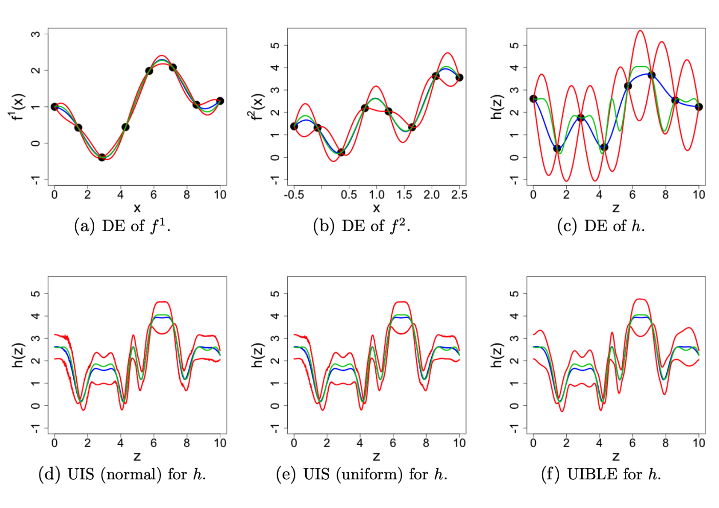
Refer to caption — Figure 3: Diagnostic plots comparing simulator output (green lines) with the DE (Section 2.2), UIS (Section 3.2.1) and UIBLE (Section 3.2.2) approaches to approximating $h$ shown as expectation (blue lines) $\pm 3$ standard deviations (red lines). For DE, the training points are represented as black dots.

Continuing the example of Section 2.3, we construct Bayes linear emulators for simulators $f^{1}$ and $f^{2}$ using training sets $\mathbf{K}$ and $\mathbf{L}$ respectively, each comprising eight simulator runs. We assume the same prior beliefs and techniques for estimating hyperparameters as discussed for $h$ in Section 2.3. The results of emulating these two simulators are shown in Figures 3d and 3e. We can see that both of these emulators are valid and accurate, with low uncertainty. The emulator for $f^{1}$ is more precise, resulting from its simpler behaviour compared to $f^{2}$ .

To combine the emulators for $f^{1}$ and $f^{2}$ using UIS we begin by evaluating $\textrm{E}_{\mathbf{K}}[f^{1}(x_{1})]$ and $\textrm{Var}_{\mathbf{K}}[f^{1}(x_{1})]$ at 1000 evenly-spaced points across the input space for $x_{1}$ . For each value of $x_{1}$ , we sampled $v=100$ possible values for $x_{2}=f^{1}(x_{1})$ according to $\mathcal{N}({\rm E}_{\mathbf{K}}[f^{1}(x_{1})],{\rm Var}_{\mathbf{K}}[f^{1}(x_{1})])$ , before calculating $\bm{\mu}_{\mathbf{h}}(\mathbf{z})$ and $\bm{\nu}_{\mathbf{h}}(\mathbf{z})$ using Equations (18) and (19). From the diagnostic results of this approximation (Figure 3d), we observe that $h$ has been emulated well, with low uncertainty. Areas of slightly larger uncertainty can be associated with regions of the input spaces for $f^{1}$ and/or $f^{2}$ with larger uncertainty, as should be expected.

To assess the effect of the chosen sampling distribution, we repeat the sampling approximation using a uniform distribution for $X_{2}$ (with parameters chosen such that the first two moments match the second-order belief specification for $f^{1}$ adjusted by $\mathbf{K}$ ). The results (Figure 3e) are fairly similar to those assuming a normal distribution, suggesting that the choice of exact distributional specification is not very influential in this case.

Uncertain Input Bayes Linear Emulation (UIBLE)

UIBLE is a computationally efficient alternative to UIS, and we profess permits reasonable approximations to simulator networks. We consider an emulator setup for $\mathbf{f}$ similar to that discussed in Section 2.1. Following Equation (1), we choose to decompose the vector of training runs $\mathbf{F}$ as follows:

\mathbf{F}=\textrm{vec}(\bm{G}\bm{B})+\mathbf{U}=\bm{W}\bm{\beta}+\mathbf{U},

where $\bm{G}=(\mathbf{g}(\mathbf{x}^{(1)}),\dots,\mathbf{g}(\mathbf{x}^{(n)}))^{T}$ is an $n\times m$ matrix of regressors at the known design points in $\mathcal{X}$ , $\bm{W}=\bm{I}_{q}\otimes\bm{G}$ , $\bm{I}_{q}$ is a $q\times q$ identity matrix, $\otimes$ represents the kronecker product, $\mathbf{U}=\mathbf{u}(\mathcal{X})$ is an $nq$ vector of residuals, and recall $\bm{\beta}=\textrm{vec}(\bm{B})$ with prior specification ${\rm E}[\bm{\beta}]=\bm{\Gamma}$ and ${\rm Var}[\bm{\beta}]=\bm{\mathit{\Delta}}$ .

We wish to make inference about $\mathbf{f}(\mathbf{X})$ , where $\mathbf{X}\in\mathbb{R}^{p}$ is an uncertain (random variable) input to $\mathbf{f}$ . Following Equation (1), $\mathbf{f}(\mathbf{X})$ can be written as

\mathbf{f}(\mathbf{X})=\mathbf{g}(\mathbf{X})^{T}\bm{B}+\mathbf{u}(\mathbf{X})=\bm{w}(\mathbf{X})\bm{\beta}+\mathbf{u}(\mathbf{X}).

where $\bm{w}(\mathbf{X})=\bm{I}_{q}\otimes\mathbf{g}(\mathbf{X})^{T}$ . We assume ${\rm E}[\mathbf{u}(\mathbf{X})]=\mathbf{0}$ and ${\rm Cov}\left[\bm{\beta},\mathbf{u}(\mathbf{X})\right]=\mathbf{0}$ . Such prior specification is similar to one that may be made in the case of known inputs (Jackson 2018). One of the key differences is specification of an appropriate correlation function that accounts for random variable inputs. We assume a general form, similar to that given by Equation (2), as follows:

{\rm Cov}\left[\mathbf{u}(\mathbf{X}),\mathbf{u}(\mathbf{X}^{\prime})\right]=c(\mathbf{X},\mathbf{X}^{\prime})\,\bm{\mathit{\Sigma}}=c({\rm E}[\mathbf{X}],{\rm Var}[\mathbf{X}],{\rm E}[\mathbf{X}^{\prime}],{\rm Var}[\mathbf{X}^{\prime}],{\rm Cov}\left[\mathbf{X},\mathbf{X}^{\prime}\right])\,\bm{\mathit{\Sigma}},

(20)

which implies that the correlation between $\mathbf{u}(\mathbf{X})$ and $\mathbf{u}(\mathbf{X}^{\prime})$ for two uncertain inputs $\mathbf{X}$ and $\mathbf{X}^{\prime}$ is a function of the second order belief specification about and between the two input variables. As an example, we propose the following extension to the Gaussian correlation function (3):

\begin{split}c(\mathbf{X},\mathbf{X}^{\prime})&=\exp\left\{-{\rm E}[(\mathbf{X}-\mathbf{X}^{\prime})^{T}\bm{\mathit{\Theta}}^{-2}(\mathbf{X}-\mathbf{X}^{\prime})]\right\}\\ &=\exp\left\{-\sum_{r=1}^{p}\left(\frac{\textrm{E}[X_{(r)}-X^{\prime}_{(r)}]^{2}+\textrm{Var}[X_{(r)}-X^{\prime}_{(r)}]}{\theta^{2}_{r}}\right)\right\}\,,\end{split}

(21)

with positive-definite diagonal matrix $\bm{\mathit{\Theta}}^{-2}$ having entries $(\Theta^{-2})_{rr}=1/\theta_{r}^{2}$ and the second line obtained from standard results on the expected value of a quadratic form (Harville 2018, pp. 200-201). This choice satisfies the desirable property that it reduces to a standard form of correlation function if $(\mathbf{X},\mathbf{X}^{\prime})=(\mathbf{x},\mathbf{x}^{\prime})$ are known. We also derive two further important results for this new correlation function in the form of two lemmas, proofs of which can be found in the supplementary material.

Lemma 3.2.1

For random variables $\mathbf{X},\mathbf{X}^{\prime}$ with finite first and second moments, the kernel function $c(\mathbf{X},\mathbf{X}^{\prime})$ from (21) is positive-definite.

Lemma 3.2.2

Covariance function (20), with $c(\mathbf{X},\mathbf{X}^{\prime})$ given by (21), is a lower bound under the Loewner (partial) ordering on the covariance obtained by assuming the conditional covariance

{\rm Cov}\left[\mathbf{u}(\mathbf{X}),\mathbf{u}(\mathbf{X}^{\prime})\,|\,\mathbf{X}=\mathbf{x},\mathbf{X}^{\prime}=\mathbf{x}^{\prime}\right]=\exp\left\{-\sum_{r=1}^{p}\left(\frac{x_{(r)}-x^{\prime}_{(r)}}{\theta_{r}}\right)^{2}\right\}\,\bm{\mathit{\Sigma}}\,.

(22)

Moreover, the $kk$ th element of (20) is a lower bound on the expected value, with respect to $\mathbf{X},\mathbf{X}^{\prime}$ , of the $kk$ th element of (22) ( $k=1,\ldots q$ ).

Whilst the proposed correlation function of Equation (21) can be viewed simply as a modelling assumption, Lemma 3.2.2 shows that it can also be derived as an approximation to the conditional covariance between $\mathbf{u}(\mathbf{X})$ and $\mathbf{u}(\mathbf{X}^{\prime})$ assuming the standard Gaussian correlation function that one might use for known $\mathbf{x},\mathbf{x}^{\prime}$ . In terms of an emulator, this quantity reflects the amount of resolved uncertainty given the training runs, hence an underestimation (lower bound) of this quantity is preferable to an overestimation. Similar derivations could be made to extend many other correlation function forms commonly presented in the literature (for example, given by Paulo 2005).

Given the general correlation function form of Equation (20) and the prior specification above, we have that ${\rm E}[\mathbf{U}]=\mathbf{0}$ , ${\rm Var}[\mathbf{U}]=\bm{\mathit{\Omega}}=\bm{\mathit{\Sigma}}\otimes\bm{C}$ and ${\rm Cov}\left[\bm{\beta},\mathbf{U}\right]=\bm{\mathit{0}}$ , where we define

\bm{C}=\left(\begin{array}[]{cccc}c(\mathbf{x}_{1},\mathbf{x}_{1})&c(\mathbf{x}_{1},\mathbf{x}_{2})&\cdots&c(\mathbf{x}_{1},\mathbf{x}_{n})\\ c(\mathbf{x}_{2},\mathbf{x}_{1})&c(\mathbf{x}_{2},\mathbf{x}_{2})&\cdots&c(\mathbf{x}_{2},\mathbf{x}_{n})\\ \vdots&\vdots&\ddots&\vdots\\ c(\mathbf{x}_{n},\mathbf{x}_{1})&c(\mathbf{x}_{n},\mathbf{x}_{2})&\cdots&c(\mathbf{x}_{n},\mathbf{x}_{n})\end{array}\right).

We also define $\bm{v}(\mathbf{X})=\bm{\mathit{\Sigma}}\otimes\mathbf{c}(\mathbf{X})$ and $\mathbf{c}(\mathbf{X})=(c(\mathbf{X},\mathbf{x}_{1}),\dots,c(\mathbf{X},\mathbf{x}_{n}))$ . We now proceed to state the adjusted belief formulae for $\mathbf{f}(\mathbf{X})$ by $\mathbf{F}$ in the form of two lemmas, proofs of which can be found in the supplementary material.

Lemma 3.2.3

The expected value of $\mathbf{f}(\mathbf{X})$ , adjusted by $\mathbf{F}$ , is given by:

{\rm E}_{\mathbf{F}}[\mathbf{f}(\mathbf{X})]={\rm E}[\bm{w}(\mathbf{X})]\,{\rm E}_{\mathbf{F}}[\bm{\beta}]+\bm{v}(\mathbf{X})\,\bm{\mathit{\Omega}}^{-1}\,(\mathbf{F}-\bm{W}\,{\rm E}_{\mathbf{F}}[\bm{\beta}])\,.

(23)

Lemma 3.2.4

The variance of $\mathbf{f}(\mathbf{X})$ , adjusted by $\mathbf{F}$ , is given by:

$\displaystyle{\rm Var}_{\mathbf{F}}[\mathbf{f}(\mathbf{X})]$	$\displaystyle=$	$\displaystyle{\rm E}[\bm{w}(\mathbf{X})\,{\rm Var}_{\mathbf{F}}[\bm{\beta}]\,\bm{w}(\mathbf{X})^{T}]+{\rm E}_{\mathbf{F}}[\bm{\beta}^{T}]\,{\rm Var}[\bm{w}(\mathbf{X})]\,{\rm E}_{\mathbf{F}}[\bm{\beta}]+\,\bm{\mathit{\Sigma}}$	(24)
		$\displaystyle\,\,\,\,\,\,\,-\,\bm{v}(\mathbf{X})\,\bm{\mathit{\Omega}}^{-1}\,\bm{v}(\mathbf{X})^{T}+\bm{v}(\mathbf{X})\,\bm{\mathit{\Omega}}^{-1}\,\bm{W}\,{\rm Var}_{\mathbf{F}}[\bm{\beta}]\,\bm{W}^{T}\,\bm{\mathit{\Omega}}^{-1}\,\bm{v}(\mathbf{X})^{T}$
		$\displaystyle\,\,\,\,\,\,\,-\,{\rm E}[\bm{w}(\mathbf{X})]\,{\rm Var}_{\mathbf{F}}[\bm{\beta}]\,\bm{W}\,\bm{\mathit{\Omega}}^{-1}\,\bm{v}(\mathbf{X})^{T}$
		$\displaystyle\,\,\,\,\,\,\,-\,({\rm E}[\bm{w}(\mathbf{X})]\,{\rm Var}_{\mathbf{F}}[\bm{\beta}]\,\bm{W}\,\bm{\mathit{\Omega}}^{-1}\,\bm{v}(\mathbf{X})^{T})^{T}\,.$

Specification of ${\rm E}[\bm{w}(\mathbf{X})]$ and ${\rm Var}[\bm{w}(\mathbf{X})]$ is straight forward for first-order linear regression functions. It is also possible for further functions of the input components, but these transformed input components will require a sensible second-order specification. As for the common known input case, vague priors on $\bm{\beta}$ result in ${\rm E}_{\mathbf{F}}[\bm{\beta}]=\bm{I}_{q}\otimes((\bm{G}^{T}\,\bm{C}^{-1}\,\bm{G})^{-1}\,\bm{G}^{T}\,\bm{C}^{-1}\,\mathbf{F})$ and ${\rm Var}_{\mathbf{F}}[\bm{\beta}]=\bm{I}_{q}\otimes(\bm{G}^{T}\,\bm{C}^{-1}\,\bm{G})^{-1}$ .

The results of Lemmas 3.2.3 and 3.2.4 can be used to provide a second-order approximation of the output of any simulator at random variable input for which a second-order belief specification is itself provided. As a result, UIBLE can be used to approximate arbitrarily large networks of simulators, where the random input $\mathbf{X}$ to one simulator is taken to have a second-order belief specification arising from a previous emulator. In this case, the most straightforward approach to obtaining ${\rm E}[\bm{w}(\mathbf{X})]$ and ${\rm Var}[\bm{w}(\mathbf{X})]$ in Equation (42) is by emulating the transformed inputs $\bm{w}(\mathbf{X})$ as further output quantities of the previous simulator.

In the setting of an emulator network formed from a chain of two simulators, estimators for $\mathbf{h}(\mathbf{z})$ are explicitly given by application of Equations (23) and (42):

	$\displaystyle\bm{\mu}_{\mathbf{h}}(\mathbf{z})$	$\displaystyle=$	$\displaystyle{\rm E}_{\mathbf{L}}[\mathbf{f}^{2}(\mathbf{X}_{2})]$		(25)
	$\displaystyle\bm{\nu}_{\mathbf{h}}(\mathbf{z})$	$\displaystyle=$	$\displaystyle{\rm Var}_{\mathbf{L}}[\mathbf{f}^{2}(\mathbf{X}_{2})]$		(26)

with ${\rm E}[\mathbf{X}_{2}]={\rm E}_{\mathbf{K}}[\mathbf{f}^{1}(\mathbf{x})]$ and ${\rm Var}[\mathbf{X}_{2}]={\rm Var}_{\mathbf{K}}[\mathbf{f}^{1}(\mathbf{x})]$ .

Illustrative Example

We emulate $f^{1}$ at 1000 evenly-spaced points $x_{1}=z$ across the input space to obtain ${\rm E}_{\mathbf{K}}[f^{1}(z)]$ and ${\rm Var}_{\mathbf{K}}[f^{1}(z)]$ . The UIBLE for $f^{2}$ is trained using the same training runs as in the previous sections, resulting in the same values for the parameters $\sigma^{2}_{2}$ and $\theta_{2}$ , where we denote by $\sigma^{2}_{i}$ and $\theta_{i}$ the scale variance and correlation length parameters for simulator $f^{i}$ respectively. Given these parameters, we can now approximate the output to $h$ at each corresponding uncertain input $X_{2}$ using Equations (25) and (26) with adjusted second-order belief specification ${\rm E}[X_{2}]={\rm E}_{\mathbf{L}}[f^{1}(z)]$ and ${\rm Var}[X_{2}]={\rm Var}_{\mathbf{L}}[f^{1}(z)]$ at each $z$ of interest. The results of doing this are shown in Figure 3f.

The result of approximating $h$ using UIBLE is slightly different to that obtained using UIS. The blue-line prediction is very similar, however, the $\pm 3$ standard deviation bounds are slightly wider in places. On the whole, however, we notice that the prediction is quite accurate, with much lower uncertainty than the DE approach used in Figure 3c.

4 Application to a Dispersion Dose-Response Chain of Simulators

In this section, we apply the UIS and UIBLE methodologies to the Dispersion Dose-Response (DDR) simulator network introduced in Section 1, comparing these approaches with DE.

Recall that the dispersion model $d(\cdot)$ (Brook et al. 2003) takes input $\mathbf{z}$ representing wind speed ( $z_{WS}$ ), wind direction ( $z_{WD}$ ) and source mass ( $z_{SM}$ ), and outputs a biological agent dose $d(\mathbf{z})$ at a spatial location of interest. Due to the behaviour of $d(\cdot)$ , we chose to emulate a transformation of the output, namely $f^{1}(\mathbf{x}_{1})=\log(d(\mathbf{x}_{1})+1)$ , treating this transformed function $f^{1}(\cdot)$ as the first simulator of the network.

The DR simulator $\rho(\cdot)$ takes dose as input and outputs a number of casualties, however, to be consistent with $f^{1}(\cdot)$ , we consider the second simulator to be $f^{2}(x_{2})=\rho(\exp(x_{2})-1)$ , so that $h(\mathbf{z})=f^{2}(f^{1}(\mathbf{z}))=\rho(d(\mathbf{z}))$ . We also note that whilst $d(\cdot)$ is computationally expensive, dose-response model $\rho(\cdot)$ is not; however we emulate both simulators to demonstrate the efficacy of our methods. Our methods are also applicable and effective when only a subset of the simulators in a network require emulation. As $f^{2}(\cdot)$ here is straightforward to emulate, our application also effectively demonstrates the use of the methods for this special case.

The composite simulator $h=f^{2}\cdot f^{1}=\rho\cdot d$ takes wind speed, wind direction and source mass as input $\mathbf{z}$ , and directly outputs a number of casualties $h(\mathbf{z})$ . The DAG of this setup can be presented as that on the right of Figure 2, with $\mathbf{f}^{1}$ and $\mathbf{f}^{2}$ (now scalar output) as discussed above. An expanded DAG showing the links between the original simulators $d$ and $\rho$ , their inputs, output and corresponding physical quantities, is presented in Figure 1.

We proceeded to construct Bayes linear emulators for each of the component simulators $f^{1}$ and $f^{2}$ , as well as the composite simulator $h$ . Ranges of interest of the inputs to simulator $f^{1}$ (and thus $h$ ) are $(z_{WD},z_{WS},z_{SM})\in[37,63]^{\circ}\times[1,150]\textrm{ms}^{-1}\times[0.001,1]\textrm{kg}$ , each of which were scaled to $[-1,1]$ for the purposes of our analysis. We constructed a training point design for $f^{1}$ and $h$ using a maximin Latin hypercube of size 50 across the three input dimensions. In contrast, simulator $f^{2}$ is one-dimensional, thus the need for fewer training points, so we take a random sample of 20 points from a uniform distribution. For each of the emulators for $f^{1},f^{2}$ and $h$ , we assumed a Gaussian correlation function, as given by Equation (3), along with a first-order polynomial mean function. We represent the scalar variance parameter and correlation length vectors as $\sigma^{2}_{1},\sigma^{2}_{2},\sigma^{2}_{h}$ and $\bm{\theta}_{1},\theta_{2},\bm{\theta}_{h}$ respectively. We fit these parameters using maximum likelihood for each emulator, this permitting a fair comparison between the emulation methods presented.

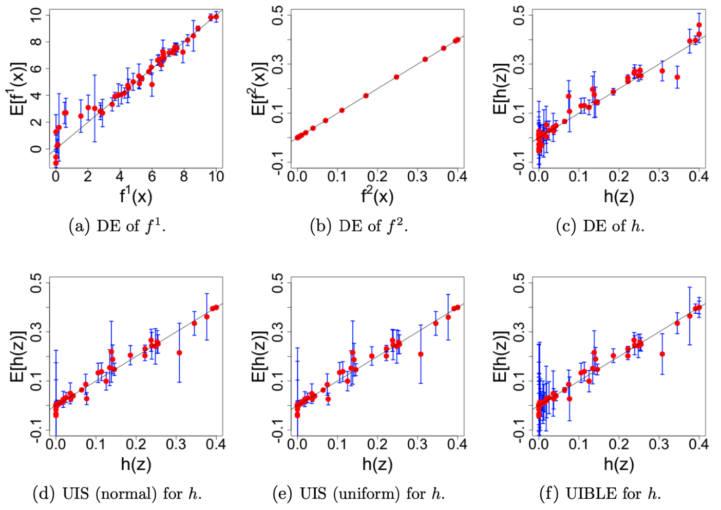
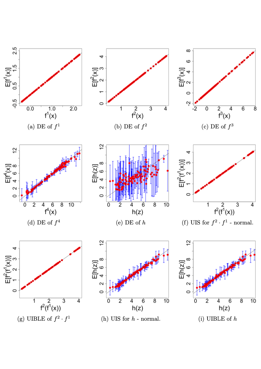
Given the component emulators for $f^{1}$ and $f^{2}$ , we can then combine them using UIS and UIBLE to yield chained emulators for $h$ . Figure 4 shows plots of adjusted expectation $\pm 3$ standard deviations against simulator output for a set of diagnostic runs for six different approximations; DE of $f^{1}$ , $f^{2}$ and $h$ , then approximation of $h$ via UIS (using normal and uniform sampling distributions) and UIBLE. The input designs for these diagnostic runs (of size 50 for $f^{1}$ and $h$ and 20 for $f^{2}$ ) were constructed in the same manner as the training run designs. In addition to the plots, Table 1 shows the Mean Absolute Standardised Prediction Error (MASPE) (Goldstein & Wooff 2007):

\frac{1}{n}\sum_{k=1}^{n}\frac{|f(\mathbf{x}^{(k)})-\mu_{f}(\mathbf{x}^{(k)})|}{\sqrt{\nu_{f}(\mathbf{x}^{(k)})}},

(27)

Root Mean Squared Prediction Error (RMSPE) (Bastos & O’Hagan 2008):

\sqrt{\frac{1}{n}\sum_{k=1}^{n}(f(\mathbf{x}^{(k)})-\mu_{f}(\mathbf{x}^{(k)}))^{2}},

(28)

and Mean Generalised Entropy Score (MGES), as defined by Equation (27) of gneiting2007sps:

-\,\frac{1}{n}\sum_{k=1}^{n}\left\{\frac{\left[f(\mathbf{x}^{(k)})-\mu_{f}(\mathbf{x}^{(k)})\right]^{2}}{\nu_{f}(\mathbf{x}^{(k)})}+\log(\nu_{f}(\mathbf{x}^{(k)}))\right\}

(29)

for the diagnostic runs for each of the six simulators, with $\mu_{f}$ , $\nu_{f}$ representing appropriate mean and variance estimators corresponding to generic simulator output $f$ . MASPE is a measure of emulator validity; heuristically we expect this value to be roughly 1 (assuming normal errors this value should be $\sqrt{2/\pi}$ ). RMSPE permits comparison of emulator accuracy. MGES is larger (better) for approximations that are both valid and precise.

Table 1: The MASPE, RMSPE and MGES for each of the six approximations discussed in Section 4. MASPE and RMSPE are smaller-the-better quantities; MGES is larger-the-better.

DE of $f^{1}$ DE of $f^{2}$ DE UIS_Normal UIS_Uniform UIBLE MASPE 1.638 0.766 1.579 1.256 1.242 0.767 RMSPE 0.6457 0.0003 0.0312 0.0235 0.0243 0.0240 MGES -1.456 14.620 4.118 7.724 7.612 6.288

We can see from Figure 4a that the emulator for $f^{1}$ is fairly accurate, with the exception of points towards the bottom end of the output range, where there are several cases of severe overestimation (with underestimated uncertainty). The emulator for $f^{2}$ (Figure 4b) is very accurate, reflecting the fact that emulator predictions can be taken with almost as much certainty as running the simulator itself. As a result, this example serves also to demonstrate the applicability of our methods of approximating simulator networks when only some of the simulators are computationally intensive enough to warrant emulating.

The direct emulator for $h$ (Figure 4c) yields predictions with underestimated uncertainty. By comparison, the estimated uncertainty for the remaining methods is larger, yielding both more appropriate MASPE values and improved MGES values. In addition, the accuracy of the predictions for the chained emulators are, on the whole, improved, this being confirmed by the RMSPE values for UIS and UIBLE. It is interesting to note, however, that the uncertainty attributed to each diagnostic point is different between the two approximations, with the uncertainty of UIBLE being larger for runs resulting in low or high values of $h(\mathbf{z})$ , and smaller for those points in the middle. This is likely to be a consequence of the way the uncertainty in $f^{1}$ is propagated through $f^{2}$ in the two methods. UIS propagates uncertainty in $f^{1}$ by sampling possible values of $f^{2}$ according to possible values of $f^{1}$ . This results in a heteroscedastic error structure across the emulator for $h$ (for example, if $f^{2}$ is expected to change little regardless of the possible values of $f^{1}$ , the uncertainty is small). In contrast, UIBLE has uncertainty from the regression part and covariance structure. As with standard Bayes linear emulation that uses a single correlation structure across $\mathbb{X}$ , there is some averaging of the uncertainty estimates for simulator prediction across the input space, even if the behaviour at some points is smoother than others. Incorporation of more sophisticated methodology into the UIBLE methodology, for example, utilising similar ideas to local GPs (Gramacy & Apley 2015), may be of benefit in this case. To summarise, we feel that the results presented give evidence for the two methods presented for linking emulators of component simulators in a network over using a direct emulator of the composite simulator in many cases. We defer further discussion to Section 6.

5 Application to a Larger Simulator Network

Both UIS and UIBLE directly generalise to more complex networks of simulators by repeated application of the general results (16), (17) or (23), (42) respectively. Such application is possible since the second-order specification resulting from application of UIS or UIBLE to one simulator leads to the sampling distribution (for UIS) or uncertain inputs specification (for UIBLE) of the next one.

In this section, we consider the illustrative network of simulators shown in Figure 5. $f^{1}$ and $f^{2}$ are taken to be the same functions as in Section 2.3, with $f^{3}$ and $f^{4}$ being defined as follows:

f^{3}(x_{3})=\sqrt{|x_{3}^{3}|}-1.6^{x_{3}},\hskip 42.67912ptf^{4}(\mathbf{x})=x_{4(1)}x_{4(3)}+\frac{x_{4(2)}}{x_{4(3)}}+\cos(x_{4(1)}+x_{4(2)}),

with $\mathbb{X}_{3}=[-4,6]$ and $\mathbb{X}_{4}=[0,4]\times[-2,8]\times[1,2.5]$ (deliberately constructed to contain the relevant output domains of previous simulators). The network function $h$ is defined by:

h(\mathbf{z})=f^{4}\big(f^{2}(f^{1}(z_{1})),f^{3}(z_{2}),z_{3}\big)

with input $\mathbf{z}=(z_{1},z_{2},z_{3})=(x_{1},x_{3},x_{4(3)})$ .

To begin with, we construct Bayes linear emulators for $f^{i},i=1,\dots,4$ , and $h$ . We take the training points for $h$ to be a Latin hypercube of size 30 across the three dimensions, appealing to the rough heuristic suggesting a minimum of $10p$ design points, where $p$ is the parameter space dimension (Loeppky et al. 2009). The relevant inputs of this Latin hypercube can then also be used as the training points for $f^{1}$ and $f^{3}$ . For $f^{2}$ and $f^{4}$ , additional training sets of 30 points were used. We again assume emulators of the form given by Equation (1) with covariance structure given by Equation (3). We specify vague prior beliefs on $\bm{\beta}$ , fitting $\sigma^{2}$ and $\bm{\theta}$ by maximum likelihood. The emulators for $f^{1}$ , $f^{2}$ , $f^{3}$ and $f^{4}$ were then combined similarly to the previous examples using both UIS (sampling from Normal distributions) and UIBLE to yield approximations for $h$ , these being compared with DE of $h$ via the diagnostic plots shown in Figures 5a-5c. The design for the diagnostic points was taken to be a Latin hypercube of size 100 across the three input dimensions to $h$ .

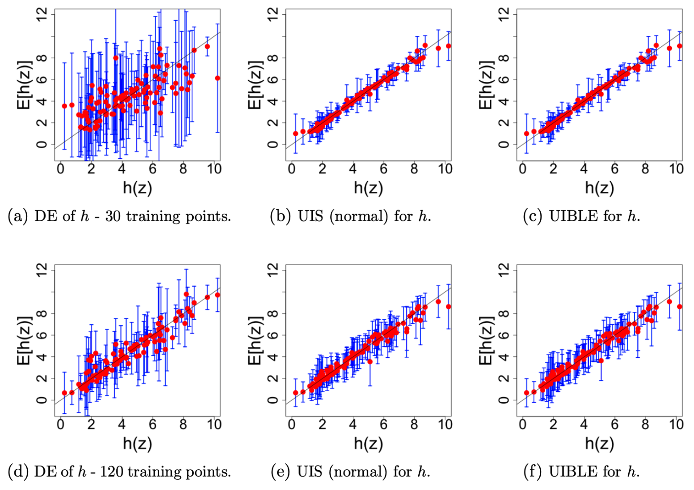
The behaviour of $h$ is hard to mimic using DE, whereas UIS and UIBLE yield much more accurate, and very similar, approximations. This is a result of the accuracy to which the component simulators can be emulated, arising largely from their reduced dimension. Diagnostic plots for the component emulators can be found in the supplementary material, along with further discussion.

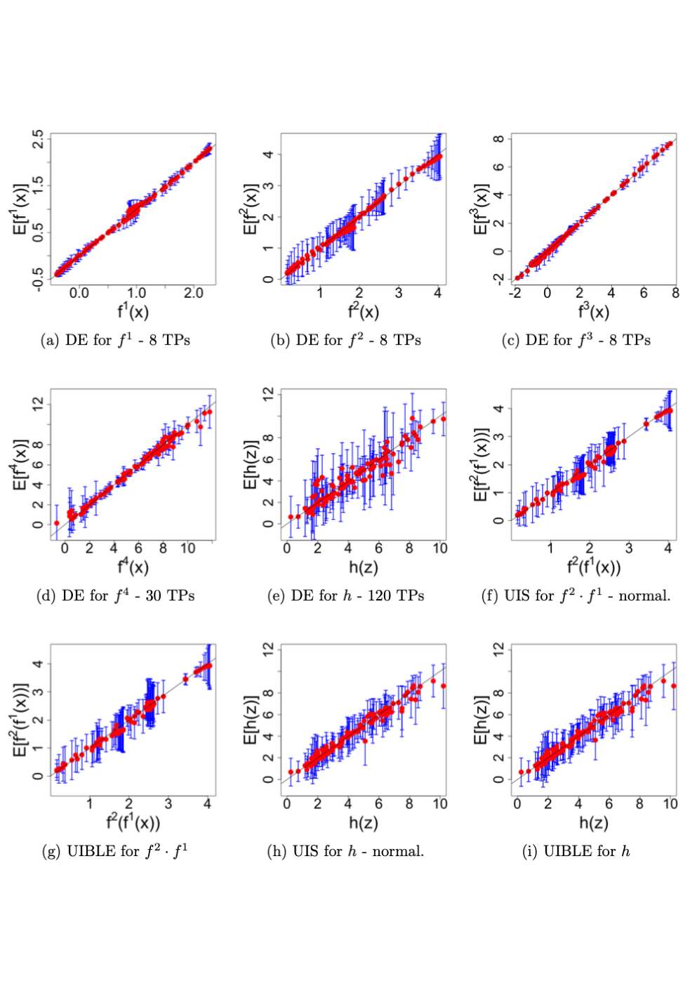
Figures 5d-5f show a repeat of the analysis shown in the top row having increased the number of training points for DE of $h$ to 120, whilst reducing the number of training points for the emulators of $f^{1}$ , $f^{2}$ and $f^{3}$ to 8 (as was the case in Sections 3.2 and 3.2). All other aspects of emulator construction remained the same. DE of $h$ using 120 training points is much more accurate than that using 30, however, only similarly accurate to UIS and UIBLE using many fewer training points. Whilst again providing evidence of the advantages of UIS and UIBLE over DE, there seems to be little discrepancy between these two proposed approaches, with the approximations being very similar. This is in contrast to the application example of Section 4, for which UIS and UIBLE yielded different, though comparably valid and accurate, results. Table 2 shows the MASPE, RMSPE and MGES (as given by Equations (27), (28) and (29) respectively) for each of the six approximations discussed above, with the numbers in brackets indicating the number of training points used to construct the emulators of the simulators in the network. These confirm the visual diagnostics presented in Figure 5. Whilst the MASPE values for UIS and UIBLE with 8 and 30 points may be a little low, we note that this slight overestimation of the uncertainty is preferable to underestimation in the context of emulation.

Table 2: The MASPE, RMSPE and MGES for each of the six approximations discussed in Section 5.

	DE (30)	UIS (30)	UIBLE (30)	DE (120)	UIS (8, 30)	UIBLE (8, 30)
MASPE	1.105	0.748	0.749	1.056	0.662	0.627
RMSPE	1.512	0.260	0.260	0.839	0.406	0.407
MGES	-19.274	1.967	1.965	-0.446	0.452	0.385

6 Discussion and Closing Remarks

We have presented novel methodology for efficient emulation of networks of simulators. Our examples have shown that both UIS and UIBLE can result in more accurate approximations compared to DE of the composite simulator of the network.

Each of the demonstrated approaches may be more applicable in different situations. UIS utilises distributional modelling assumptions for sampling purposes and thus more closely approximates a fully Bayesian analysis. Note that the Bayes linear framework in which this paper is largely set does not prevent the investigation of the consequences of assuming certain distributions. However, the sensitivity of results to the choice of sampling distribution should be explored by performing a robustness analysis. The sampling nature of UIS inherently requires running a standard emulator many times (at different points) for a single evaluation. If it is required to evaluate $\mathbf{f}(\mathbf{X})$ at very many points, then the approximations (16) and (17) could themselves be emulated using a stochastic simulator (Allen 2017; Binois et al. 2018). This would avoid the need to approximate $\mathbf{f}$ multiple times for each $\mathbf{X}$ specification.

In contrast, UIBLE is computationally more efficient as a result of each evaluation being akin to a single run of a standard emulator. The modelling assumptions (particularly regarding the correlation function form) are pragmatic but the resulting emulator can, and should, be assessed using diagnostic summaries and plots. Overall, in the examples presented, no large differences in predictive ability were found between the two methods, although in Section 4 the two approaches showed different levels of accuracy across different parts of the input space.

In addition to situations involving networks of simulators, the uncertain input emulation approaches discussed here have more general application. For example, they would permit efficient sensitivity analyses; several evaluations of an emulator with constant $\textrm{E}[\mathbf{X}]$ and varying $\textrm{Var}[\mathbf{X}]$ could quickly provide an indication of the influence of individual inputs on simulator output behaviour.

There are multiple directions for future work, for example by developing the methodology to allow for stochastic simulators and ensembles of competing simulators where model selection is required. Interesting design questions arise where several simulators are linked together. In particular, the efficiency of running the various simulators may vary, as might the number of training points deemed appropriate to capture simulator behaviour to a reasonable degree. Deciding how to allocate a fixed computational budget across computer experiments for the individual simulators is therefore an important follow on from this work. As a final thought, note that in this article we constructed the component emulators (including estimation of parameters) before combining them together. However, a combined parameter estimation process over all of the component emulators of the simulators in a network may prove to be a highly valuable addition to this research.

Acknowledgements

This work was supported by Chemical and Biological Technologies Department (contract HDTRA1-17-C-0028). We are grateful to Crystalcast project members for invaluable discussions, comments, and provision of the simulators for the dispersion dose-response application. Particular thanks are due to Professor Veronica Bowman and Dr Daniel Silk (Defence Science and Technology Laboratory, UK), and Dr Daria Semochkina (University of Southampton, UK).

References

(1)
Allen (2017) Allen, L. J. S. (2017), ‘A primer on stochastic epidemic models: Formulation, numerical simulation, and analysis’, Infectious Disease Modelling 2, 128–142.
Andrianakis & Challenor (2012) Andrianakis, Y. & Challenor, P. G. (2012), ‘The effect of the nugget on Gaussian process emulators of computer models’, Computational Statistics and Data Analysis 56, 4215–4228.
Bastos & O’Hagan (2008) Bastos, T. S. & O’Hagan, A. (2008), ‘Diagnostics for Gaussian process emulators.’, Technometrics 51, 425–438.
Binois et al. (2018) Binois, M., Huang, J., Gramacy, R. B. & Ludkovski, M. (2018), ‘Replication or exploration? sequential design for stochastic simulation experiments’, Technometrics 61(1), 7–23.
Brook et al. (2003) Brook, D. R., Beck, N. V., Clem, C. M., Strickland, D. C., Griffiths, I. H., Hall, D. J., Kingdon, R. D. & Hargrave, J. M. (2003), ‘Validation of the urban dispersion model (udm)’, International Conference on Harmonisation within Atmospheric Dispersion Modelling for Regulatory Purposes 8, 8–12.
Chebyshev (1867) Chebyshev, P. (1867), ‘Des valeurs moyennes’, Journal de mathématiques pures et appliquées 2(12), 177–184.
Damianou & Lawrence (2013) Damianou, A. C. & Lawrence, N. D. (2013), ‘Deep gaussian processes’, Proceedings of the 16th International Conference on Artificial Intelligence and Statistics 31.
de Finetti (1974) de Finetti, B. (1974), Theory of Probability, Vol. 1, Wiley.
de Finetti (1975) de Finetti, B. (1975), Theory of Probability, Vol. 2, Wiley.
Dunlop et al. (2018) Dunlop, M. M., Girolami, M. A., Stuart, A. M. & Teckentrup, A. L. (2018), ‘How deep are deep gaussian processes’, Journal of Machine Learning Research 19, 1–46.
Goldstein (1999) Goldstein, M. (1999), Bayes linear analysis, in S. Kotz, C. B. Read, N. Balakrishnan & B. Vidakovic, eds, ‘Encyclopedia of statistical Sciences’, Wiley, New York, chapter Bayes Linear Analysis, pp. 29–34.
Goldstein & Rougier (2004) Goldstein, M. & Rougier, J. C. (2004), ‘Probabilistic formulations for transferring inferences from mathematical models to physical systems’, SIAM Journal on Scientific Computing 26(2), 467–487.
Goldstein et al. (2013) Goldstein, M., Seheult, A. & Vernon, I. (2013), Assessing model adequacy, in J. Wainwright & M. Mulligan, eds, ‘Environmental Modelling: Finding Simplicity in Complexity’, John Wiley and Sons, Chichester.
Goldstein & Wooff (2007) Goldstein, M. & Wooff, D. (2007), Bayes Linear Statistics, Wiley, Chichester.
Gramacy & Apley (2015) Gramacy, R. B. & Apley, D. W. (2015), ‘Large gaussian process approximation for large computer experiments’, Journal of Computational and Graphical Statistics 24(2), 561–578.
Gramacy & Lee (2012) Gramacy, R. B. & Lee, H. K. H. (2012), ‘Bayesian treed gaussian process models with an application to computer modeling’, Journal of the American Statistical Association 103(483), 1119–1130.
Groer (1978) Groer, P. G. (1978), ‘Dose-response curves and competing risks’, Proceedings of the National Academy of Sciences of the United States of America 75(9), 4087–4091.
Hartigan (1969) Hartigan, J. A. (1969), ‘Linear Bayesian methods’, Journal of the Royal Statistical Society 31, 446–454.
Harville (2018) Harville, D. A. (2018), Linear Models and the relevant distributions and matrix algebra, CRC press, Boca Raton.
Jackson (2018) Jackson, S. E. (2018), Design of Physical System Experiments Using Bayes Linear Emulation and History Matching Methodology with Application to Arabidopsis Thaliana, PhD thesis, Durham University.
Jackson et al. (2020) Jackson, S. E., Vernon, I., Liu, J. & Lindsey, K. (2020), ‘Understanding hormonal crosstalk in arabidopsis root development via emulation and history matching’, Statistical Approaches in Genetics and Molecular Biology 19(5).
Jensen (1998) Jensen, F. V. (1998), ‘An introduction to bayesian networks’, The Knowledge Engineering Review 13(2), 201–208.
Jha & Juanes (2014) Jha, B. & Juanes, R. (2014), ‘Coupled multiphase flow and poromechanics: A computational model of pore pressure effects on fault slip and earthquake triggering’, Water Resources Research 50, 3776–3808.
Kennedy & O’Hagan (2001) Kennedy, M. C. & O’Hagan, A. (2001), ‘Bayesian calibration of computer models’, Journal of the Royal Statistical Society 63(3), 425–464.
Koehler & Owen (1996) Koehler, J. R. & Owen, A. B. (1996), ‘Computer experiments’.
Kyzyurova et al. (2018) Kyzyurova, K. N., Berger, J. O. & Wolpert, R. L. (2018), ‘Coupling computer models through linking their statistical emulators’, Journal on Uncertainty Quantification 6(3), 1151–1171.
Legrand et al. (2009) Legrand, J., Egan, J. R., Hall, I. M., Cauchemez, S., Leach, S. & Ferguson, N. M. (2009), ‘Estimating the location and spatial extent of a covert anthrax release’, PLoS Computational Biology 5(1).
Loeppky et al. (2009) Loeppky, J. L., Sacks, J. & Welch, W. J. (2009), ‘Choosing the sample size of a computer experiment: A practical guide’, Technometrics 51(4), 366–376.
Mardia et al. (1979) Mardia, K. V., Kent, J. T. & Bibby, J. M. (1979), Multivariate Analysis, Academic Press, London.
McHutchon & Rasmussen (2011) McHutchon, A. & Rasmussen, C. E. (2011), ‘Gaussian process training with input noise’, Advances in Neural Information Processing Systems 24.
O’Hagan (1987) O’Hagan, A. (1987), ‘Bayes linear estimators for randomized response models’, Journal of the American Statistical Association 82, 580–585.
Paulo (2005) Paulo, R. (2005), ‘Default priors for Gaussian processes’, The Annals of Statistics 33(2), 556–582.
Pukelsheim (1994) Pukelsheim, F. (1994), ‘The three sigma rule’, The American Statistician 48(2), 88–91.
Shawe-Taylor & Cristianini (2011) Shawe-Taylor, J. & Cristianini, N. (2011), Kernel Methods for Pattern Analysis, Cambridge University Press, Cambridge.
Taylor et al. (2012) Taylor, K. E., Stouffer, R. J. & Meehi, G. A. (2012), ‘An overview of cmip5 and the experiment design’, Journal of the American Meteorological Society 93, 485–498.
Thulasiraman & Swamy (1992) Thulasiraman, K. & Swamy, M. N. S. (1992), Graphs: Theory and Algorithms, Wiley, New York.
Titisias & Lawrence (2010) Titisias, M. K. & Lawrence, N. D. (2010), ‘Bayesian gaussian process latent variable model’, Proceedings of the 13th International Conference on Artificial Intelligence and Statistics 9, 844–851.
Whittle (1992) Whittle, P. (1992), Probability Via Expectation, Springer.

Appendix A Bayes Linear Statistics

In this article, we have largely focused on the Bayes Linear approach (Hartigan 1969, O’Hagan 1987, Goldstein 1999, Goldstein & Wooff 2007) to statistical inference, which takes expectation as primitive, following De Finetti (de Finetti 1974, de Finetti 1975, Whittle 1992), and deals with second-order belief specifications (that is, expectations, variances and covariances) of observable quantities. Probabilities can be represented as the expectation of the corresponding indicator function when required.

More precisely, suppose that there are two collections of random quantities, $\mathcal{B}=(B_{1},...,B_{r})$ and $\mathcal{D}=(D_{1},...,D_{s})$ . Bayes linear analysis involves updating subjective beliefs about $\mathcal{B}$ given observation of $\mathcal{D}$ . In order to do so, prior mean vectors and covariance matrices for $\mathcal{B}$ and $\mathcal{D}$ (that is, $\textrm{E}[\mathcal{B}]$ , $\textrm{E}[\mathcal{D}]$ , $\textrm{Var}[\mathcal{B}]$ and $\textrm{Var}[\mathcal{D}]$ ), along with a covariance matrix between $\mathcal{B}$ and $\mathcal{D}$ (that is, $\textrm{Cov}[\mathcal{B},\mathcal{D}]$ ), must be specified. Second-order beliefs about $\mathcal{B}$ can be adjusted in the light of $\mathcal{D}$ using the Bayes linear update formulae:

$\displaystyle\textrm{E}_{\mathcal{D}}[\mathcal{B}]$	$\displaystyle=$	$\displaystyle\textrm{E}[\mathcal{B}]+\textrm{Cov}[\mathcal{B},\mathcal{D}]\textrm{Var}[\mathcal{D}]^{-1}(\mathcal{D}-\textrm{E}[\mathcal{D}])$	(30)
$\displaystyle\textrm{Var}_{\mathcal{D}}[\mathcal{B}]$	$\displaystyle=$	$\displaystyle\textrm{Var}[\mathcal{B}]-\textrm{Cov}[\mathcal{B},\mathcal{D}]\textrm{Var}[\mathcal{D}]^{-1}\textrm{Cov}[\mathcal{D},\mathcal{B}]$	(31)
$\displaystyle\textrm{Cov}_{\mathcal{D}}[\mathcal{B}_{1},\mathcal{B}_{2}]$	$\displaystyle=$	$\displaystyle\textrm{Cov}[\mathcal{B}_{1},\mathcal{B}_{2}]-\textrm{Cov}[\mathcal{B}_{1},\mathcal{D}]\textrm{Var}[\mathcal{D}]^{-1}\textrm{Cov}[\mathcal{D},\mathcal{B}_{2}]$	(32)

Equations (30)-(32) are the backbone of the Bayes linear update Equations (4) and (5) of Section 2.1 of the main text. $\textrm{E}_{\mathcal{D}}[\mathcal{B}]$ and $\textrm{Var}_{\mathcal{D}}[\mathcal{B}]$ are termed the adjusted expectation and variance of $\mathcal{B}$ given $\mathcal{D}$ (Goldstein & Wooff 2007). $\textrm{Cov}_{\mathcal{D}}[\mathcal{B}_{1},\mathcal{B}_{2}]$ is termed the adjusted covariance of $\mathcal{B}_{1}$ and $\mathcal{B}_{2}$ given $\mathcal{D}$ , where $\mathcal{B}_{1}$ and $\mathcal{B}_{2}$ are subcollections of $\mathcal{B}$ . Following on from this, given a third collection of random quantities $\mathcal{A}=(A_{1},...,A_{t})$ we can sequentially adjust beliefs about $\mathcal{B}$ given observation of random quantities $\mathcal{D}$ and $\mathcal{A}$ using a sequential Bayes linear adjustment:

	$\displaystyle\textrm{E}_{\mathcal{D}\cup\mathcal{A}}[\mathcal{B}]$	$\displaystyle=$	$\displaystyle\textrm{E}_{\mathcal{D}}[\mathcal{B}]+\textrm{Cov}_{\mathcal{D}}[\mathcal{B},\mathcal{A}]\textrm{Var}_{\mathcal{D}}[\mathcal{A}]^{-1}(\mathcal{A}-\textrm{E}_{\mathcal{D}}[\mathcal{A}])$		(33)
	$\displaystyle\textrm{Var}_{\mathcal{D}\cup\mathcal{A}}[\mathcal{B}]$	$\displaystyle=$	$\displaystyle\textrm{Var}_{\mathcal{D}}[\mathcal{B}]-\textrm{Cov}_{\mathcal{D}}[\mathcal{B},\mathcal{A}]\textrm{Var}_{\mathcal{D}}[\mathcal{A}]^{-1}\textrm{Cov}_{\mathcal{D}}[\mathcal{A},\mathcal{B}]$		(34)

which adjusts the adjusted beliefs of $\mathcal{B}$ by $\mathcal{D}$ now additionally by $\mathcal{A}$ . Note that equivalent results are obtained by updating first by $\mathcal{A}$ then $\mathcal{D}$ by swapping the occurrences of $\mathcal{D}$ and $\mathcal{A}$ in Equations (30)-(34) above. Equations (33) and (34) are important for some of the discussions and calculations presented throughout Section 3 of the main text.

Appendix B Proof of Lemmas 3.2.1-3.2.4

In this section, we prove Lemmas 1 - 4 of the main text.

Proof of Lemma 3.2.1

Rewrite Equation (21) as

\begin{split}c(\mathbf{X},\mathbf{X}^{\prime})&=\exp\left\{-{\rm E}[(\mathbf{X}-\mathbf{X}^{\prime})^{T}\Theta^{-2}(\mathbf{X}-\mathbf{X}^{\prime})]\right\}\\ &=\exp\left\{-{\rm E}[\mathbf{X}^{T}\Theta^{-2}\mathbf{X}]\right\}\exp\left\{-{\rm E}[(\mathbf{X}^{\prime})^{T}\Theta^{-2}\mathbf{X}^{\prime}]\right\}\exp\left\{2{\rm E}[\mathbf{X}^{T}\Theta^{-2}\mathbf{X}^{\prime}]\right\}\,,\\ \end{split}

with kernel

k(\mathbf{X},\mathbf{X}^{\prime})=\exp\left\{2{\rm E}[\mathbf{X}^{T}\Theta^{-2}\mathbf{X}^{\prime}]\right\}\,.

The kernel $k(\mathbf{X},\mathbf{X}^{\prime})$ is positive definite since

\mathrm{tr}(\Theta^{-2}{\rm Var}[\mathbf{X}])+{\rm E}[\mathbf{X}]^{T}\Theta^{-2}{\rm E}[\mathbf{X}]\geq 0

with equality if and only if $\mathbf{X}$ has a degenerate distribution at zero. Postive definiteness of the function $c(\mathbf{X},\mathbf{X}^{\prime})$ then follows from standard properties of kernels (see Shawe-Taylor & Cristianini 2011, ch. 3)

Proof of Lemma 3.2.2

Covariance can be derived from conditional quantities using the law of total covariance, hence:

{\rm Cov}\left[\mathbf{u}(\mathbf{X}),\mathbf{u}(\mathbf{X}^{\prime})\right]={\rm E}[{\rm Cov}\left[\mathbf{u}(\mathbf{X}),\mathbf{u}(\mathbf{X}^{\prime})\,|\,\mathbf{X}=\mathbf{x},\mathbf{X}^{\prime}=\mathbf{x}^{\prime}\right]]\\ +{\rm Cov}\left[{\rm E}[\mathbf{u}(\mathbf{X})\,|\,\mathbf{X}],{\rm E}[\mathbf{u}(\mathbf{X}^{\prime})\,|\,\mathbf{X}^{\prime}]\right]\,.

Under the assumption that ${\rm E}[\mathbf{u}(\mathbf{X})]=0$ , it follows that ${\rm Cov}\left[{\rm E}[\mathbf{u}(\mathbf{X})\,|\,\mathbf{X}],{\rm E}[\mathbf{u}(\mathbf{X}^{\prime})\,|\,\mathbf{X}^{\prime}]\right]=0$ . Hence for conditional covariance (22), we have

\begin{split}{\rm Cov}\left[\mathbf{u}(\mathbf{X}),\mathbf{u}(\mathbf{X}^{\prime})\right]&=\mathrm{E}\left[\exp\left(-\sum_{r=1}^{p}\left\{\frac{X_{(r)}-X^{\prime}_{(r)}}{\theta_{r}}\right\}^{2}\right)\right]\,\bm{\mathit{\Sigma}}\\ &\succeq\exp\left(-\sum_{r=1}^{p}\mathrm{E}\left[\left\{\frac{X_{(r)}-X^{\prime}_{(r)}}{\theta_{r}}\right\}^{2}\,\right]\right)\,\bm{\mathit{\Sigma}}\,,\\ \end{split}

under the Loewner (partial) ordering, following from an application of Jensen’s inequality and the positive-definiteness of $\bm{\mathit{\Sigma}}$ . As the diagonal entries of $\bm{\mathit{\Sigma}}$ are all non-negative, elementwise inequality for the $kk$ th entry follows directly ( $k=1,\ldots,q$ ).

Proof of Lemma 3.2.3

We begin by expanding the terms of the Bayes linear update as follows:

\displaystyle{\rm E}_{\mathbf{F}}[\mathbf{f}(\mathbf{X})]

\displaystyle=

\displaystyle{\rm E}_{\mathbf{F}}[\bm{w}(\mathbf{X})\,\bm{\beta}]+{\rm E}_{\mathbf{F}}[\mathbf{u}(\mathbf{X})]\,.

Taking the two parts of the right-hand side of this equation separately, we first have that

{\rm E}_{\mathbf{F}}[\bm{w}(\mathbf{X})\,\bm{\beta}]={\rm E}_{\mathbf{F}}[\bm{w}(\mathbf{X})]\,{\rm E}_{\mathbf{F}}[\bm{\beta}]={\rm E}[\bm{w}(\mathbf{X})]\,{\rm E}_{\mathbf{F}}[\bm{\beta}]\,,

(35)

where we have used the facts that ${\rm E}_{\mathbf{F}}[\bm{w}(\mathbf{X})]={\rm E}[\bm{w}(\mathbf{X})]$ since ${\rm Cov}\left[\mathbf{X},\mathbf{F}\right]=\mathbf{0}$ , and ${\rm Cov}_{\mathbf{F}}\left[\bm{w}(\mathbf{X}),\bm{\beta}\right]=\mathbf{0}$ since ${\rm Cov}_{\mathbf{F}}\left[\mathbf{g}(\mathbf{X}),\bm{\beta}\right]=\mathbf{0}$ . We then have, using basic rules of linear algebra (Mardia et al. 1979), that

$\displaystyle{\rm E}_{\mathbf{F}}[\mathbf{u}(\mathbf{X})]$	$\displaystyle=$	$\displaystyle{\rm E}[\mathbf{u}(\mathbf{X})]+{\rm Cov}\left[\mathbf{u}(\mathbf{X}),\mathbf{F}\right]\,{\rm Var}[\mathbf{F}]^{-1}\,(\mathbf{F}-{\rm E}[\mathbf{F}])$	(36)
	$\displaystyle=$	$\displaystyle{\rm Cov}\left[\mathbf{u}(\mathbf{X}),\mathbf{U}\right]\,{\rm Var}[\mathbf{F}]^{-1}\,(\mathbf{F}-\bm{W}\,\bm{\Gamma})$
	$\displaystyle=$	$\displaystyle\bm{v}(\mathbf{X})\,(\bm{W}\,\bm{\mathit{\Delta}}\,\bm{W}^{T}+\bm{\mathit{\Omega}})^{-1}\,(\mathbf{F}-\bm{W}\,\bm{\Gamma})$
	$\displaystyle=$	$\displaystyle\bm{v}(\mathbf{X})\,\big((\bm{W}\,\bm{\mathit{\Delta}}\,\bm{W}^{T}+\bm{\mathit{\Omega}})^{-1}\,\mathbf{F}-(\bm{W}\,\bm{\mathit{\Delta}}\,\bm{W}^{T}+\bm{\mathit{\Omega}})^{-1}\,\bm{W}\,\bm{\Gamma}\big)$
	$\displaystyle=$	$\displaystyle\bm{v}(\mathbf{X})\bigg(\big(\bm{\mathit{\Omega}}^{-1}-\bm{\mathit{\Omega}}^{-1}\,\bm{W}\,(\bm{\mathit{\Delta}}^{-1}+\bm{W}^{T}\,\bm{\mathit{\Omega}}^{-1}\,\bm{W})^{-1}\,\bm{W}^{T}\,\bm{\mathit{\Omega}}^{-1}\big)\,\mathbf{F}$
		$\displaystyle\,\,\,\,\,\,-\bm{\mathit{\Omega}}^{-1}\,\bm{W}\,(\bm{W}^{T}\,\bm{\mathit{\Omega}}^{-1}\,\bm{W}+\bm{\mathit{\Delta}}^{-1})^{-1}\,\bm{\mathit{\Delta}}^{-1}\,\bm{W}\bigg)$
	$\displaystyle=$	$\displaystyle\bm{v}(\mathbf{X})\,\bm{\mathit{\Omega}}^{-1}\,\big(\mathbf{F}-\bm{W}\,(\bm{\mathit{\Delta}}^{-1}+\bm{W}^{T}\,\bm{\mathit{\Omega}}^{-1}\,\bm{W})^{-1}\,(\bm{\mathit{\Delta}}^{-1}\,\bm{W}+\bm{W}\,\bm{\mathit{\Omega}}^{-1}\,\mathbf{F})\big)$
	$\displaystyle=$	$\displaystyle\bm{v}(\mathbf{X})\,\bm{\mathit{\Omega}}^{-1}\,(\mathbf{F}-\bm{W}\,{\rm E}_{\mathbf{F}}[\bm{\beta}])\,.$

Combining Equations (35) and (36) we get:

\displaystyle{\rm E}_{\mathbf{F}}[\mathbf{f}(\mathbf{X})]

\displaystyle=

\displaystyle{\rm E}[\bm{w}(\mathbf{X})]\,{\rm E}_{\mathbf{F}}[\bm{\beta}]+\bm{v}(\mathbf{X})\,\bm{\mathit{\Omega}}^{-1}\,(\mathbf{F}-\bm{W}\,{\rm E}_{\mathbf{F}}[\bm{\beta}])\,.

$\Box$

Proof of Lemma 3.2.4

We begin by expanding the terms of the Bayes linear update as follows:

$\displaystyle{\rm Var}_{\mathbf{F}}[\mathbf{f}(\mathbf{X})]$	$\displaystyle=$	$\displaystyle{\rm Var}_{\mathbf{F}}[\bm{w}(\mathbf{X})\,\bm{\beta}+\mathbf{u}(\mathbf{X})]$	(37)
	$\displaystyle=$	$\displaystyle{\rm Var}_{\mathbf{F}}[\bm{w}(\mathbf{X})\,\bm{\beta}]+{\rm Var}_{\mathbf{F}}[\mathbf{u}(\mathbf{X})]$
		$\displaystyle\,\,\,\,\,\,\,+\,{\rm Cov}_{\mathbf{F}}\left[\bm{w}(\mathbf{X})\,\bm{\beta},\mathbf{u}(\mathbf{X})\right]+{\rm Cov}_{\mathbf{F}}\left[\mathbf{u}(\mathbf{X}),\bm{w}(\mathbf{X})\,\bm{\beta}\right]\,.$

Taking each term on the right-hand side of Equation (37) in turn, we have, using linear algebra (Mardia et al. 1979):

	$\displaystyle{\rm Var}_{\mathbf{F}}[\bm{w}(\mathbf{X})\,\bm{\beta}]$	$\displaystyle=$	$\displaystyle{\rm E}[{\rm Var}_{\mathbf{F}\cup\mathbf{X}}[\bm{w}(\mathbf{X})\,\bm{\beta}]]+{\rm Var}[{\rm E}_{\mathbf{F}\cup\mathbf{X}}[\bm{w}(\mathbf{X})\,\bm{\beta}]]$		(38)
		$\displaystyle=$	$\displaystyle{\rm E}[\bm{w}(\mathbf{X})\,{\rm Var}_{\mathbf{F}}[\bm{\beta}]\,\bm{w}(\mathbf{X})^{T}]+{\rm E}_{\mathbf{F}}[\bm{\beta}^{T}]\,{\rm Var}[\bm{w}(\mathbf{X})]{\rm E}_{\mathbf{F}}[\bm{\beta}]\,,$		(38)

$\displaystyle{\rm Var}_{\mathbf{F}}[\mathbf{u}(\mathbf{X})]$			(39)
	$\displaystyle=$	$\displaystyle{\rm Var}[\mathbf{u}(\mathbf{X})]-{\rm Cov}\left[\mathbf{u}(\mathbf{X}),\mathbf{F}\right]\,{\rm Var}[\mathbf{F}]^{-1}\,{\rm Cov}\left[\mathbf{F},\mathbf{u}(\mathbf{X})\right]$
	$\displaystyle=$	$\displaystyle\bm{\mathit{\Sigma}}-\bm{v}(\mathbf{X})\,(\bm{W}\,\bm{\mathit{\Delta}}\,\bm{W}^{T}+\bm{\mathit{\Omega}})^{-1}\,\bm{v}(\mathbf{X})^{T}$
	$\displaystyle=$	$\displaystyle\bm{\mathit{\Sigma}}-\bm{v}(\mathbf{X})\,(\bm{\mathit{\Omega}}^{-1}-\bm{\mathit{\Omega}}^{-1}\,\bm{W}\,(\bm{\mathit{\Delta}}^{-1}+\bm{W}^{T}\,\bm{\mathit{\Omega}}^{-1}\,\bm{W})^{-1}\,\bm{W}^{T}\,\bm{\mathit{\Omega}}^{-1})\,\bm{v}(\mathbf{X})^{T}$
	$\displaystyle=$	$\displaystyle\bm{\mathit{\Sigma}}-\bm{v}(\mathbf{X})\,\bm{\mathit{\Omega}}^{-1}\,\bm{v}(\mathbf{X})^{T}+\bm{v}(\mathbf{X})\,\bm{\mathit{\Omega}}^{-1}\,\bm{W}\,{\rm Var}_{\mathbf{F}}[\bm{\beta}]\,\bm{W}^{T}\,\bm{\mathit{\Omega}}^{-1}\,\bm{v}(\mathbf{X})^{T}\,,$

and

	$\displaystyle{\rm Cov}_{\mathbf{F}}\left[\bm{w}(\mathbf{X})\,\bm{\beta},\mathbf{u}(\mathbf{X})\right]$				(40)
		$\displaystyle=$	$\displaystyle{\rm Cov}\left[\bm{w}(\mathbf{X})\,\bm{\beta},\mathbf{u}(\mathbf{X})\right]-{\rm Cov}\left[\bm{w}(\mathbf{X})\,\bm{\beta},\mathbf{F}\right]{\rm Var}[\mathbf{F}]^{-1}{\rm Cov}\left[\mathbf{F},\mathbf{u}(\mathbf{X})\right]\,.$		(40)

In Equation (40), we have that:

$\displaystyle{\rm Cov}\left[\bm{w}(\mathbf{X})\,\bm{\beta},\mathbf{F}\right]$	$\displaystyle=$	$\displaystyle{\rm Cov}\left[\bm{w}(\mathbf{X})\,\bm{\beta},\bm{W}\,\bm{\beta}\right]$
	$\displaystyle=$	$\displaystyle{\rm Cov}\left[\bm{w}(\mathbf{X})\,\bm{\beta},\bm{\beta}\right]\bm{W}^{T}$
	$\displaystyle=$	$\displaystyle({\rm E}[\bm{w}(\mathbf{X})\,\bm{\beta}\,\bm{\beta}^{T}]-{\rm E}[\bm{w}(\mathbf{X})\,\bm{\beta}]{\rm E}[\bm{\beta}^{T}])\bm{W}^{T}$
	$\displaystyle=$	$\displaystyle({\rm E}[\bm{w}(\mathbf{X})]{\rm E}[\bm{\beta}\,\bm{\beta}^{T}]-{\rm E}[\bm{w}(\mathbf{X})]{\rm E}[\bm{\beta}]{\rm E}[\bm{\beta}^{T}])\bm{W}^{T}$
	$\displaystyle=$	$\displaystyle{\rm E}[\bm{w}(\mathbf{X})]{\rm Var}[\bm{\beta}]\bm{W}^{T}$
	$\displaystyle=$	$\displaystyle{\rm E}[\bm{w}(\mathbf{X})]\bm{\mathit{\Delta}}\bm{W}^{T}\,,$

so that

$\displaystyle{\rm Cov}_{\mathbf{F}}\left[\bm{w}(\mathbf{X})\,\bm{\beta},\mathbf{u}(\mathbf{X})\right]$	$\displaystyle=$	$\displaystyle-\,{\rm E}[\bm{w}(\mathbf{X})]\,\bm{\mathit{\Delta}}\,\bm{W}^{T}(\bm{W}\,\bm{\mathit{\Delta}}\,\bm{W}^{T}+\bm{\mathit{\Omega}})^{-1}\bm{v}(\mathbf{X})^{T}$	(41)
	$\displaystyle=$	$\displaystyle-\,{\rm E}[\bm{w}(\mathbf{X})](\bm{W}^{T}\,\bm{\mathit{\Omega}}^{-1}\,\bm{W}+\bm{\mathit{\Delta}}^{-1})^{-1}\bm{W}\,\bm{\mathit{\Omega}}^{-1}\,\bm{v}(\mathbf{X})^{T}$
	$\displaystyle=$	$\displaystyle-\,{\rm E}[\bm{w}(\mathbf{X})]{\rm Var}_{\mathbf{F}}[\bm{\beta}]\bm{W}^{T}\,\bm{\mathit{\Omega}}^{-1}\bm{v}(\mathbf{X})^{T}\,.$

Putting Equations (38), (39) and (41) together, we get that:

$\displaystyle{\rm Var}_{\mathbf{F}}[\mathbf{f}(\mathbf{X})]$	$\displaystyle=$	$\displaystyle{\rm E}[\bm{w}(\mathbf{X})\,{\rm Var}_{\mathbf{F}}[\bm{\beta}]\,\bm{w}(\mathbf{X})^{T}]+{\rm E}_{\mathbf{F}}[\bm{\beta}^{T}]\,{\rm Var}[\bm{w}(\mathbf{X})]\,{\rm E}_{\mathbf{F}}[\bm{\beta}]+\,\bm{\mathit{\Sigma}}$	(42)
		$\displaystyle\,\,\,\,\,\,\,-\,\bm{v}(\mathbf{X})\,\bm{\mathit{\Omega}}^{-1}\,\bm{v}(\mathbf{X})^{T}+\bm{v}(\mathbf{X})\,\bm{\mathit{\Omega}}^{-1}\,\bm{W}\,{\rm Var}_{\mathbf{F}}[\bm{\beta}]\,\bm{W}^{T}\,\bm{\mathit{\Omega}}^{-1}\,\bm{v}(\mathbf{X})^{T}$
		$\displaystyle\,\,\,\,\,\,\,-\,{\rm E}[\bm{w}(\mathbf{X})]\,{\rm Var}_{\mathbf{F}}[\bm{\beta}]\,\bm{W}\,\bm{\mathit{\Omega}}^{-1}\,\bm{v}(\mathbf{X})^{T}$
		$\displaystyle\,\,\,\,\,\,\,-\,({\rm E}[\bm{w}(\mathbf{X})]\,{\rm Var}_{\mathbf{F}}[\bm{\beta}]\,\bm{W}\,\bm{\mathit{\Omega}}^{-1}\,\bm{v}(\mathbf{X})^{T})^{T}$

$\Box$

Appendix C Extension of the Networks Example

Figure 6 shows diagnostic plots for nine emulators relating to the larger simulator network example Section 5 of the main text, using 30 training points to train each emulator. Figures 6a-6e show diagnostic plots for DE of $f^{1},f^{2},f^{3},f^{4}$ and $h$ . Since $f^{1}$ , $f^{2}$ and $f^{3}$ are relatively simple 1-dimensional functions, 30 training points allow almost-perfect predictions. $f^{4}$ is emulated with some uncertainty but fairly accurately, however, it is difficult to mimic the behaviour of $h$ using DE. Figures 6f and 6g show diagnostic plots for the approximation of $f^{2}(f^{1}(\cdot))$ using UIS and UIBLE. Both result in highly accurate and precise emulators as a result of the accuracy and precision of the component emulators for $f^{1}$ and $f^{2}$ (diagnostics shown in Figures 6a and 6b). Figures 6h and 6i show diagnostic plots for the approximation of $h$ using UIS and UIBLE, these being identical to Figures 5b and 5c of the main text, but shown again here for comparison purposes.

Figure 7 shows nine corresponding diagnostic plots for the case of reducing the number of training points for the emulators of the one-dimensional simulators $f^{1}$ , $f^{2}$ and $f^{3}$ to 8, whilst increasing the number for $h$ to 120. Whilst $f^{1}$ and $f^{3}$ still have fairly low uncertainty, the uncertainty on $f^{2}$ is higher, though all three emulators have high accuracy. As discussed in the main text, DE for $h$ constructed using 120 training points is much more accurate, although only similarly accurate to UIS and UIBLE (Figures 7h and 7i) using many fewer points. The uncertainties in the approximation of $f^{2}(f^{1}(\cdot))$ using UIS and UIBLE reflect accurate and fairly precise predictions, and are in accordance with the alternative 1-dimensional diagnostic plots shown in Figures 3d and 3f of the main text.