A Framework for Generating Synthetic Distribution Feeders using OpenStreetMap PubID: pubid: 978-1-7281-0407-2/19/$31.00 ©2019 IEEE Thanks: This work was partially supported by the Office of Naval Research under Award Number N00014-18-1-2393 and the Engineering Research Center Program of the National Science Foundation and the Office of Energy Efficiency and Renewable Energy of the Department of Energy under NSF Cooperative Agreement Number EEC-1041895.

A recent study developing synthetic radial distribution feeders [7] views the distribution system as a random graph with nodes and edges that can be imbued with various properties following realistic statistics for the topology and parameters, derived from a large set of real feeders. The approach includes an analysis and a synthesis step. The analysis step identifies statistical distributions between properties such as load, node, degree or cable length using data from the Netherlands. The statistics are then input to a synthesis algorithm that creates feeders with similar topological and physical characteristics; importantly, the statistical trends for different operating conditions of voltage, phase angles power flows are also realistic. Moreover, [7] provides a method for validating the results, using metrics of statistical similarity such as the Kulback Leibler distance of the trends of the real and synthetic cases. Another line of work is based on the Reference Network Model (RNM) [8], a large-scale distribution planning tool that can help regulators to estimate efficient costs in the context of incentives and regulation applied to distribution companies. The synthetic test-cases developed using RNM allows for the simultaneous planning of high-, medium-, and low-voltage networks using simultaneity factors and lays out cables in urban areas, taking street map into consideration. An adaptation of RNM to create RNM-US is shown in [9] which provides full-scale, high-quality synthetic distribution system dataset(s) for testing distribution automation algorithms, distributed control approaches, and other emerging distribution technologies. Broad application of RNM is hindered by the significant amount of data required such as (a) geo-referenced for transmission, substations, and consumer data, (b) load profiles, (c) equipment library for all power system components, (d) technical and economic parameters governing operation, and (e) environmental and topography data.

The contribution of this paper is threefold: 1) substation locations are selected from the ACTIVS models [3], a set of geo-embedded synthetic models of the US transmission system, to enable joint evaluation of synthetic transmission and distribution systems; 2) following the assumption that power distribution network follows the road network; radial positive sequence synthetic distribution feeder topologies are generated using OpenStreetMap (a constantly expanding publicly available data source for road network) [11] to create a spatially embedded dataset; 3) loads are assigned to nodes in the distribution network using US census population data. The developed framework also has the capability to provide the distribution feeder model in OpenDSS [12] format allowing simulation capabilities like hosting capacity calculation [13], complex infrastructure network simulation [14], and more.

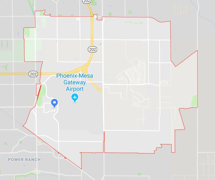
Location information (longitude, latitude) of the substation from ACTIVS cases is used to identify the corresponding ZIP Code ($Z$) from the ”US 2010 Census Bureau ZIP Code” shapefile¹¹ 1 A shapefile is a simple, non-topological format for storing the geometric location and attribute information of geographic features. [15] or the Google Reverse Geocoding API [16] if unavailable in the shapefile. If both processes fail, then the closest ZIP Code to substation $N$ is assigned. The selected substation for demonstration belongs to the ZIP Code $85212$. Fig. 2 illustrates the territory of ZIP Code $85212$ from Google Maps.

1. (i)

   A ZIP Code can be served by multiple substations. Using ACTIVS, the set of substation(s) ($N_{Z}$) in $Z$ are retrieved, giving $N\in N_{Z}\in N_{D}$. For ZIP Code $85212$, the ACTIVS case returns two substations with positive net loads, the second one to be located at $(33.3376^{\circ},-111.5900^{\circ})$ with a load demand of $55.07~+j8.51~\textnormal{MVA}$.

2. (ii)

   The ’drive’ network (drivable public streets excluding service roads) for $Z$ is retrieved using [17]. The retrieved network is a directional graph ($G_{Z}$) with self-loops and parallel edges.

3. (iii)

   $G_{Z}$ is then split into Voronoi regions [18] where the number of Voronoi partitions $\mathinner{\!\left\lvert N_{Z}\right\rvert}$ equals to number of substations in ZIP Code $Z$²² 2 $\mathinner{\!\left\lvert\bullet\right\rvert}$ of a set represents the cardinality of the set.. Fig. 3a shows $G_{Z}$ for the ZIP Code $85212$ having two substations with positive net loads. The blue and black colored circles represent the location of substations in $85212$. Fig. Fig. 3a also illustrates the two Voronoi regions corresponding to the two substations. The red and green nodes are distribution feeder nodes inside the blue and black substation’s Voronoi regions, respectively. The edges marked in red in Fig. 3a are the edges connecting the two Voronoi regions.

4. (iv)

   $\mathinner{\!\left\lvert N_{Z}\right\rvert}$ number of sub-graphs ($g_{z}$) are then created from $G_{Z}$ by splitting along the edges connecting the Voronoi regions. A sub-graph only includes the strongly connected nodes [19]; hence the sub-graph creation process can create isolated nodes as shown in Fig. 3a. The isolated nodes either have degree 0 or are part of an isolated graph. Let $G_{Z}^{n},~g_{z}^{n}$ be the set of nodes for $G_{Z}$, sub-graph $g_{z}$ respectively while $I$ is the set of isolated nodes. It follows that $I=G_{Z}^{n}\setminus\cup_{z=1}^{\mathinner{\!\left\lvert N_{Z}\right\rvert}}g_{z}^{n}$, where $\cup_{z=1}^{\mathinner{\!\left\lvert N_{Z}\right\rvert}}g_{z}^{n}$ represents the union of all the sub-graph nodes. Using Algorithm 1 the isolated nodes are connected to the appropriate sub-graph ($g_{z}$) as shown in Fig. 3b.

   1: for each node $i\in I$ do

   2:   find $A_{i}$ where $A_{i}$ is the set of nodes adjacent to node $i$ in $G_{z}$

   3:   find the $k^{th}$ sub-graph $g_{z,k}$ for the first node $a$ such that $a\in A_{i}\cap g^{n}_{z,k}$

   4:   connect node $i$ to node $a$ and copy the node and edge properties from $G_{Z}$ to $g^{n}_{z,k}$

   5:   remove $i$ from $I$

   6: end for

5. (v)

   A minimum spanning tree using Kruskal’s algorithm [20] is calculated for each $g_{z}$.

6. (vi)

   The census block data for $Z$ is retrieved using US 2010 Census data. If $B_{Z}$ is the set of census blocks for ZIP Code $Z$, there are $\mathinner{\!\left\lvert B_{Z}\right\rvert}$ census blocks within $Z$. There are $662$ census blocks for ZIP code $85212$, i.e. $\mathinner{\!\left\lvert B_{Z}\right\rvert}=662$.

7. (vii)

   For every node in $\cup_{z}g_{z}$, the framework finds the census block that a node belongs to using the latitude and longitude information of the node and geometry of census blocks.

8. (viii)

   The framework then assigns a weight ($p_{w}^{n}$) to each node based on the population information of the census block the node belongs to. For instance, if node $(n)$ belongs to census block $b_{z}^{i}\in B_{Z}$,  $p_{w}^{n}=\dfrac{m(b_{z}^{i})}{\sum_{i=1}^{\mathinner{\!\left\lvert B_{Z}\right\rvert}}m(b_{z}^{i})}$, where $m(b_{z}^{i})$ returns the population of the census block $b_{z}^{i}$. For $85212$, total population, or $\sum_{i=1}^{\mathinner{\!\left\lvert B_{Z}\right\rvert}}m(b_{z}^{i})$, is $25015$.

The output of these steps is a set of sub-graphs $\{g_{z}\}$ with $\mathinner{\!\left\lvert N_{Z}\right\rvert}$ elements where sub-graph $g_{z,N}$ corresponds to substation $N$ and $g_{z,N}\in\{g_{z}\}$.

1. (i)

   The node closest to the location of substation $N$ is chosen to be the slack bus/ substation node for distribution feeder for the sub-graph/ feeder $g_{z,N}$. The big red circle in Fig. 4 indicates the substation node.

2. (ii)

   The substation demand is then distributed among the nodes of the sub-graph $g_{z,N}$. Zero load nodes are identified using the methodology in [7]. The substation node is designated to have zero load. The load distribution for each node under the sub-graph $g_{z,N}$ is equated using the following equations:

   $\displaystyle P(n)$

   $\displaystyle=P_{N}\left(\dfrac{1}{n}+\epsilon\right)\times p_{w}^{n}~;~Q(n)$

   $\displaystyle=Q_{N}\left(\dfrac{1}{n}+\epsilon\right)\times p_{w}^{n}$

   (1)

   Here, $P_{N}$ and $Q_{N}$ are the real and reactive power load demand of substation $N$, respectively, and $\epsilon$ can be chosen from any distribution such as uniform distribution, or t-location scale distribution as in [7]. The final $P(n)$ and $Q(n)$ values are then scaled using the following equations to match the total demand $P_{N}$ and $Q_{N}$.

   $\displaystyle P(n)$

   $\displaystyle=P_{N}\times\dfrac{P(n)}{\sum P(n)}~;~Q(n)$

   $\displaystyle=Q_{N}\times\dfrac{Q(n)}{\sum Q(n)}$

   (2)

   The developed framework does not necessarily require population information for modeling the feeder. Setting the value of $p_{w}^{n}$ to 1 for all nodes will ignore the effect of population on the load distribution. Figure 4 shows the heat-map of real power of $g_{z,N}$ done following a t-location scale distribution while excluding the population information.

   

The framework has a radial graph $g_{z,N}$ of lines with known length, a substation node, and the real and reactive power demand at each node. Bus $0$ denotes the substation node or the point of common coupling (PCC), with a predefined reference voltage ($v_{0}$). Additional parameters including line resistance and reactance are required to run a steady state power flow.

Following the lossless linearized distribution power flow or DistFlow equations from [21] and using symbols introduced in Table I, for every $(i,j)\in\cal L$ of the radial distribution feeder:

Equation (3a)-(3b) can be used to calculate the vector of real and reactive power flows for every line using the nodal demand values. By using a predefined cable database (that includes impedance and apparent power (MVA) carrying capacity information) and the calculated line flows, the framework then follows Algorithm 2 to find the appropriate cable that can meet the power flow through a line with minimum number of parallels. Assigning cables allows the calculation of $r_{ij}$ and $x_{ij}$ for all lines, and equation (3c) is then used to calculate nodal voltages using $v_{0}=1.00.$

If the minimum of the node voltages is less than a predefined voltage threshold ($v_{th}$), nodes with degree 1 are removed from $g_{z,N}$ and procedures described in II-C and II-D are repeated for the modified version of the graph $g_{z,N}$.

Output of the previous step is then converted to an OpenDSS model to calculate a non-linear power flow solution for the positive sequence network model. The framework models all the loads as constant power loads with load and cable information retrieved from the graph $g_{z,N}$. Using the non-linear power flow provides the loss values across the network. The steady state voltage profile for the OpenDSS model is shown in Fig. 5.

The OpenDSS simulation returns loss values of $3.95832~+j7.63604~\textnormal{MVA}$; hence active losses are $8.9\%$ of the load demand of $40.47~+j11.14~\textnormal{MVA}$. The non-linear power flow solution from OpenDSS , which accounts for the losses, has larger currents, which are responsible for dragging the voltage profile lower than that calculated by the DistFlow equation (3c).

• •

  $\mathcal{C}_{N}$ represents the set of single phase nodes.

• •

  $d_{AB},d_{BC},d_{CA}$ represent the difference of total power of phase A and phase B; phase B and phase C ; phase C and phase A respectively.

• •

  $u_{n}^{A},u_{n}^{B},u_{c}^{C}$ represent the binary variables corresponding to individual phase for node $n$.

• •

  $p_{n}$ represents the real power demand of node $n\in\mathcal{C}_{N}$.

Figure. 6 shows the distribution feeder with three-phase and single-phase edges.

References

- [1] K. P. Schneider, Y. Chen, D. Engle, and D. Chassin, “A taxonomy of north american radial distribution feeders,” in 2009 IEEE Power Energy Society General Meeting, July 2009, pp. 1–6.
- [2] F. E. Postigo Marcos, C. M. Domingo, T. G. San Roman, B. S. Palmintier, B.-M. Hodge, V. K. Krishnan, F. de Cuadra Garcia, and B. A. Mather, “A review of power distribution test feeders in the united states and the need for synthetic representative networks,” Energies (Basel), vol. 10, no. 11, 11 2017.
- [3] A. B. Birchfield, T. Xu, K. M. Gegner, K. S. Shetye, and T. J. Overbye, “Grid structural characteristics as validation criteria for synthetic networks,” IEEE Transactions on Power Systems, vol. 32, no. 4, pp. 3258–3265, July 2017.
- [4] K. M. Gegner, A. B. Birchfield, , K. S. Shetye, and T. J. Overbye, “A methodology for the creation of geographically realistic synthetic power flow models,” in 2016 IEEE Power and Energy Conference at Illinois (PECI), Feb 2016, pp. 1–6.
- [5] H. Li, A. L. Bornsheuer, T. Xu, A. B. Birchfield, and T. J. Overbye, “Load modeling in synthetic electric grids,” in 2018 IEEE Texas Power and Energy Conference (TPEC), Feb 2018, pp. 1–6.
- [6] S. Abeysinghe, J. Wu, and M. Sooriyabandara, “A statistical assessment tool for electricity distribution networks,” Energy Procedia, vol. 105, pp. 2595 – 2600, 2017, 8th International Conference on Applied Energy, ICAE2016, 8-11 October 2016, Beijing, China. [Online]. Available: http://www.sciencedirect.com/science/article/pii/S187661021730810X
- [7] E. Schweitzer, A. Scaglione, A. Monti, and G. A. Pagani, “Automated generation algorithm for synthetic medium voltage radial distribution systems,” IEEE Journal on Emerging and Selected Topics in Circuits and Systems, vol. 7, no. 2, pp. 271–284, June 2017.
- [8] C. Mateo Domingo, T. Gomez San Roman, . Sanchez-Miralles, J. P. Peco Gonzalez, and A. Candela Martinez, “A reference network model for large-scale distribution planning with automatic street map generation,” IEEE Transactions on Power Systems, vol. 26, no. 1, pp. 190–197, Feb 2011.
- [9] V. K. Krishnan, B. S. Palmintier, B. S. Hodge, E. T. Hale, T. Elgindy, B. Bugbee, M. N. Rossol, A. J. Lopez, D. Krishnamurthy, C. Vergara, C. M. Domingo, F. Postigo, F. de Cuadra, T. Gomez, P. Duenas, M. Luke, V. Li, M. Vinoth, and S. Kadankodu, “Smart-ds: Synthetic models for advanced, realistic testing: Distribution systems and scenarios,” 8 2017.
- [10] A. B. Birchfield, E. Schweitzer, M. Athari, T. Xu, T. J. Overbye, A. Scaglione, and Z. Wang, “A metric-based validation process to assess the realism of synthetic power grids,” Energies, vol. 10, no. 8, p. 1233, Aug 2017.
- [11] OpenStreetMap contributors, “Planet dump retrieved from https://planet.osm.org ,” https://www.openstreetmap.org, 2017.
- [12] EPRI, “OpenDSS.” [Online]. Available: http://smartgrid.epri.com/SimulationTool.aspx
- [13] M. H. J. Bollen and S. K. Rönnberg, “Hosting capacity of the power grid for renewable electricity production and new large consumption equipment,” Energies, Aug 2017.
- [14] J. M. Brase and D. L. Brown, “Modeling, simulation and analysis of complex networked systems,” May 2009.
- [15] U.S. Census Bureau, 2010. [Online]. Available: {https://www.census.gov/geographies/mapping-files/time-series/geo/tiger-line-file.2010.html}
- [16] Google, “Reverse geocoding.” [Online]. Available: https://developers.google.com/maps/documentation/javascript/examples/geocoding-reverse
- [17] G. Boeing, “OSMnx: New methods for acquiring, constructing, analyzing, and visualizing complex street networks,” Computers, Environment and Urban Systems, vol. 65, pp. 126 – 139, 2017.
- [18] Voronoi Diagram. [Online]. Available: {https://courses.cs.washington.edu/courses/cse326/00wi/projects/voronoi.html}
- [19] Strongly Connected Components. [Online]. Available: {https://networkx.github.io/documentation/networkx-1.9/reference/generated/networkx.algorithms.components.strongly_connected.strongly_connected_components.html}
- [20] Minimum Spanning Tree. [Online]. Available: {https://networkx.github.io/documentation/networkx-1.10/reference/generated/networkx.algorithms.mst.minimum_spanning_tree.html}
- [21] M. Farivar, L. Chen, and S. Low, “Equilibrium and dynamics of local voltage control in distribution systems,” in 52nd IEEE Conference on Decision and Control, Dec 2013, pp. 4329–4334.