∎

DYTurbo: Fast predictions for Drell–Yan processesJournal: Eur. Phys. J. C

Stefano Camarda^∗¹ Maarten Boonekamp² Giuseppe Bozzi³ Stefano Catani⁴ Leandro Cieri⁵ Jakub Cuth⁶ Giancarlo Ferrera⁷ Daniel de Florian⁸ Alexandre Glazov⁹ Massimiliano Grazzini¹⁰ Manuella G. Vincter¹¹ Matthias Schott⁶

Abstract

Drell–Yan lepton pair production processes are extremely important for Standard Model (SM) precision tests and for beyond the SM searches at hadron colliders. Fast and accurate predictions are essential to enable the best use of the precision measurements of these processes; they are used for parton density fits, for the extraction of fundamental parameters of the SM, and for the estimation of background processes in searches. This paper describes a new numerical program, DYTurbo, for the calculation of the QCD transverse-momentum resummation of Drell–Yan cross sections up to next-to-next-to-leading logarithmic accuracy combined with the fixed-order results at next-to-next-to-leading order ( $\mathcal{O}(\alpha_{\mathrm{S}}^{2})$ ), including the full kinematical dependence of the decaying lepton pair with the corresponding spin correlations and the finite-width effects. The DYTurbo program is an improved reimplementation of the DYqT, DYRes and DYNNLO programs, which provides fast and numerically precise predictions through the factorisation of the cross section into production and decay variables, and the usage of quadrature rules based on interpolating functions for the integration over kinematic variables.

Keywords:

Hadron colliders Electroweak QCD Drell–Yan

1 Introduction

The Drell–Yan process denotes massive lepton-pair production in hadron-hadron collisions at high energies, as proposed by Sidney D. Drell and Tung-Mow Yan in 1970 PhysRevLett.25.902.2, and first observed at the Alternating Gradient Synchrotron PhysRevLett.25.1523. At the Large Hadron Collider (LHC) 1748-0221-3-08-S08001, the Drell–Yan process continues to play a fundamental role in probing the proton parton distribution functions (PDF), thereby providing valuable information on the $u$ - and $d$ -quark valence PDFs Khachatryan:2016pev and insight into the light-quark sea decomposition, in particular on the $s$ - over $\bar{d}$ -quark ratio Aaboud:2016btc. This process is also used to measure fundamental electroweak parameters such as the mass of the $W$ boson Aaboud:2017svj, the weak-mixing angle Aad:2015uau; Chatrchyan:2011ya, and the $W$ -boson width Camarda:2016twt. An accurate modelling of the Drell–Yan process is of paramount importance for searches of new physics phenomena beyond the Standard Model (SM) in final states with high dilepton invariant mass Khachatryan:2016zqb; Khachatryan:2016jww; Aaboud:2016cth; Aaboud:2016zkn. These experimental measurements need to be compared to accurate predictions based on high-order perturbative QCD and electroweak corrections. The Drell-Yan production total cross section and the vector boson rapidity distribution have been analytically computed up to the next-to-next-to-leading order (NNLO) in powers of the QCD coupling $\alpha_{\mathrm{S}}$ in Refs. Hamberg:1990np; Harlander:2002wh and Anastasiou:2003ds, respectively. Fully exclusive parton-level NNLO calculations, which include the leptonic decay of the vector boson, have been implemented in publicly available Monte Carlo codes Melnikov:2006di; Melnikov:2006kv; Catani:2009sm; Catani:2010en. The transverse-momentum ( $q_{\mathrm{T}}$ ) distribution of the lepton pair at large (formally, non-vanishing) values of $q_{\mathrm{T}}$ can be evaluated at $O(\alpha_{\mathrm{S}}^{3})$ from the parton-level calculations of $W$ / $Z/\gamma^{*}$ + jet production that have been performed in Refs. Boughezal:2015dva; Ridder:2015dxa; Boughezal:2015ded; Boughezal:2016dtm; Gehrmann-DeRidder:2017mvr. Various calculations that combine the QCD resummation formalism of logarithmically enhanced contributions at small- $q_{\mathrm{T}}$ Dokshitzer:1978yd; Parisi:1979se; Collins:1984kg; Catani:2013tia with fixed-order perturbative results at different levels of theoretical accuracy have been performed in Refs. Balazs:1997xd; Ellis:1997sc; Ellis:1997ii; Bozzi:2010xn; Banfi:2012du; Guzzi:2013aja; Catani:2015vma; Bizon:2018foh; Bizon:2019zgf. Analogous resummed calculations have been performed by applying Soft Collinear Effective Theory methods Becher:2010tm; Becher:2011xn; Chiu:2012ir; Ebert:2016gcn; Becher:2019bnm and transverse-momentum dependent factorisation Collins:2011zzd; GarciaEchevarria:2011rb; Collins:2012uy; Collins:2014jpa; Scimemi:2017etj; Bertone:2019nxa; Bacchetta:2019tcu; Bacchetta:2018lna; Bozzi:2019vnl. Electroweak (EW) Dittmaier:2001ay; Baur:2004ig; Zykunov:2006yb; Arbuzov:2005dd; CarloniCalame:2006zq; Baur:2001ze; Zykunov:2005tc; CarloniCalame:2007cd; Arbuzov:2007db and mixed QCD-EW Kotikov:2007vr; Kilgore:2011pa; Dittmaier:2014qza; Bonciani:2016wya; Cieri:2018sfk; deFlorian:2018wcj; Delto:2019ewv radiative corrections have also been considered. A reliable estimate of the theoretical uncertainties requires various procedures, which also include variations of PDFs, renormalisation and factorisation scales, and SM parameters. It is thus necessary to rely on computing codes that allow fast calculations of these variations with small numerical uncertainties. The DYTurbo program, which is presented in this paper, aims at providing fast and numerically precise predictions of the Drell–Yan production cross sections, for phenomenological applications such as QCD analyses and extraction of fundamental parameters of the SM. The enhancement in performance over original programs is achieved by overhauling pre-existing codes, by factorising the differential cross section into production and decay variables, and by introducing the usage of one-dimensional and multi-dimensional numerical integration based on interpolating functions. The DYTurbo program is a reimplementation of the DYRes Catani:2015vma and DYqT Bozzi:2010xn programs for $q_{\mathrm{T}}$ resummation, and of the DYNNLO Catani:2009sm program for the finite-order perturbative QCD calculation up to NNLO. The DYRes Catani:2015vma and DYqT Bozzi:2010xn programs encode the $q_{\mathrm{T}}$ resummed cross sections up to next-to-next-to-leading-logarithmic (NNLL) accuracy by using the resummation formalism proposed in Refs. Catani:2000vq; Bozzi:2005wk; Bozzi:2007pn. The $W$ +jet and $Z/\gamma^{*}$ +jet predictions at $O(\alpha_{\mathrm{S}})$ and $O(\alpha_{\mathrm{S}}^{2})$ are reimplemented from the analytical calculations of Refs. Ellis:1981hk; Arnold:1988dp; Gonsalves:1989ar, as encoded in DYqT, for the case of the triple-differential production cross sections as a function of rapidity $y$ , invariant mass $m$ , and transverse momentum $q_{\mathrm{T}}$ of the lepton pair, and from the MCFM program Campbell:2010ff, as encoded in DYRes and DYNNLO, for the full kinematical dependence of the decaying leptons. Software profiling was employed to achieve code optimisation. The most successful optimisation strategies leading to significant performance improvement were hoisting loop-invariant expressions out of loops, removing conditional statements from loops to allow the compiler performing automatic loop vectorisation, and manual loop unrolling. The DYTurbo software is based on a modular C++ structure, with a few Fortran functions wrapped and interfaced to C++. Multi-threading is implemented with OpenMP, and through the Cuba library by means of fork/wait system calls Hahn:2014fua. A flexible user interface allows setting the parameters of the calculation through input files and command line options. The results are provided in the form of text files and ROOT histograms Brun:1997pa. Preliminary versions of the DYTurbo program were used by the ATLAS Collaboration in Refs. Aaboud:2017svj; Aaboud:2016zpd; ATLAS-CONF-2018-037. The DYTurbo program is publicly available github.

2 Predictions with DYTurbo

The DYTurbo program provides predictions for $W$ and $Z/\gamma^{*}$ -boson (collectively denoted as $V$ -boson) production cross sections, fully differential in the four momenta of the decay leptons, and inclusive over final-state QCD radiation. The cross sections can be computed by performing the resummation of logarithmically-enhanced contributions in the small- $q_{\mathrm{T}}$ region of the leptons pairs at leading-logarithmic (LL), next-to-leading-logarithmic (NLL), and NNLL accuracy, and also including the corresponding finite-order QCD contributions at next-to-leading order (NLO) and NNLO. The logarithmically-enhanced terms are resummed by using the resummation formalism of Ref. Bozzi:2005wk in impact-parameter space. The structure of the cross section calculations is summarised in Eqs. (1) and (4), and we refer the reader to the discussion in Refs. Catani:2015vma; Bozzi:2010xn; Catani:2009sm for details on the theoretical formulation. Upon integration of final-state QCD radiation, the fully-differential Drell–Yan cross section is described by six kinematic variables corresponding to the momenta of the two leptons. To the purpose of reducing the complexity of the calculation, it is useful to reorganise the fully-differential Drell–Yan cross section by factorising the dynamics of the boson production, and the kinematics of the boson decay. The cross section is therefore expressed as a function of the transverse momentum $q_{\mathrm{T}}$ , the rapidity $y$ and the invariant mass $m$ of the lepton pair, and three angular variables corresponding to the polar angle $\theta_{\ell}$ and azimuth $\phi_{\ell}$ of the lepton decay in a given boson rest frame and to the azimuth $\phi_{V}$ of the boson in the laboratory frame. However, the cross section does not depend on $\phi_{V}$ , since in unpolarised hadron collisions the initial-state hadrons, i.e. the incoming beams, are to very good approximation azimuthally symmetric. Therefore the dependence of the cross section on $\phi_{V}$ is not considered further. In the following a distinction will be made between fiducial cross sections, where kinematic requirements are applied on the final state leptons, and total or full-lepton phase space cross sections. The former requires the evaluation of the fivefold differential cross sections, the latter are ( $q_{\mathrm{T}}$ , $m$ , $y$ )-dependent triple-differential cross sections integrated over $\cos\theta_{\ell}$ and $\phi_{\ell}$ . At NLL+NLO and NNLL+NNLO, the $q_{\mathrm{T}}$ -resummed cross section for $V$ -boson production can be written as

\displaystyle\textrm{d}\sigma^{\textrm{V}}_{\textrm{(N)NLL+(N)NLO}}

\displaystyle=

\displaystyle\textrm{d}\sigma^{\textrm{res}}_{\textrm{(N)NLL}}-\textrm{d}\sigma^{\textrm{asy}}_{\textrm{(N)LO}}+\textrm{d}\sigma^{\textrm{f.o.}}_{\textrm{(N)LO}}\,,

(1)

where $\textrm{d}\sigma^{\textrm{res}}$ is the resummed component of the cross-section, $\textrm{d}\sigma^{\textrm{asy}}$ is the asymptotic term that represents the fixed-order expansion of $\textrm{d}\sigma^{\textrm{res}}$ , and $\textrm{d}\sigma^{\textrm{f.o.}}$ is the $V$ +jet finite-order cross section integrated over final-state QCD radiation. All the cross sections are differential in $q_{\mathrm{T}}^{2}$ . The resummed component $\textrm{d}\sigma^{\textrm{res}}$ is the most important term at small $q_{\mathrm{T}}$ . The finite-order term $\textrm{d}\sigma^{\textrm{f.o.}}$ gives the larger net contribution at large $q_{\mathrm{T}}$ . The fixed-order expansion of the resummed component $\textrm{d}\sigma^{\textrm{asy}}$ embodies the singular behaviour of the finite-order term, providing a smooth behaviour of Eq. (1) as $q_{\mathrm{T}}$ approaches zero. The two finite-order terms of Eq. (1) and the finite-order factor $\mathcal{H}^{\textrm{V}}_{\textrm{(N)NLO}}$ in $\textrm{d}\sigma^{\textrm{res}}$ (see Eq. (2)) are calculated up to the same power in $\alpha_{\mathrm{S}}$ . The resummed component and its fixed-order expansion are given by ¹¹ 1 The convolution with PDFs and the sum over different initial-state partonic contributions are implied in the shorthand notation of Eqs. (2), (3) and (5). Analogously, the inverse Fourier transformation from $b$ space to $q_{\mathrm{T}}$ space is implied in Eq. (2).

	$\displaystyle\textrm{d}\sigma^{\textrm{res}}_{\textrm{(N)NLL}}$	$\displaystyle=$	$\displaystyle\textrm{d}{\hat{\sigma}}^{\textrm{V}}_{\textrm{LO}}(q_{\mathrm{T}})\times\mathcal{H}^{\textrm{V}}_{\textrm{(N)NLO}}\times\exp\{\mathcal{G}_{\textrm{(N)NLL}}\}$		(2)
	$\displaystyle\textrm{d}\sigma^{\textrm{asy}}_{\textrm{(N)LO}}$	$\displaystyle=$	$\displaystyle\textrm{d}{\hat{\sigma}}^{\textrm{V}}_{\textrm{LO}}(q_{\mathrm{T}})\times\Sigma^{\textrm{V}}(q_{\mathrm{T}}/Q)_{\textrm{(N)LO}}\,,$		(3)

where $Q$ denotes the auxiliary resummation scale Bozzi:2005wk that is introduced in $\textrm{d}\sigma^{\textrm{res}}$ and, consistently, in $\textrm{d}\sigma^{\textrm{asy}}$ . The term $\textrm{d}{\hat{\sigma}}^{\textrm{V}}_{\textrm{LO}}(q_{\mathrm{T}})$ is the leading-order (LO) cross section evaluated for non-vanishing values of $q_{\mathrm{T}}$ according to a given $q_{\mathrm{T}}$ -recoil prescription Catani:2015vma, namely, with values of $\theta_{\ell}$ and $\phi_{\ell}$ that correspond to a chosen dilepton rest frame. The factor $\mathcal{H}^{V}$ is the hard-collinear coefficient function. The term $\mathcal{G}$ is the exponent of the Sudakov form factor and it is originally expressed as a function of the impact parameter $b$ , which is the Fourier-conjugate variable to $q_{\mathrm{T}}$ . This term embodies the resummation of the logarithmically-enhanced contributions at LL, NLL or NNLL accuracy in $b$ space. In order to parameterise non-perturbative QCD effects, the Sudakov form factor includes a non-perturbative contribution, whose simplest form is a Gaussian form factor. The $b$ space expression of the Sudakov form factor is then evaluated in $q_{\mathrm{T}}$ space by numerically performing the (inverse) Fourier transformation. The function $\Sigma^{\textrm{V}}(q_{\mathrm{T}}/Q)$ arises from the finite-order expansion of $\mathcal{H}^{\textrm{V}}\times\exp\{\mathcal{G}\}$ , and it matches the singular behaviour of $\textrm{d}\sigma^{\textrm{f.o.}}$ in the region $q_{\mathrm{T}}\to 0$ . An additional feature of the DYTurbo program is the possibility of computing finite-order cross sections at LO, NLO and NNLO without the resummation of logarithmically-enhanced contributions. At NLO and NNLO, the finite-order cross section for $V$ -boson production is computed by using the $q_{\mathrm{T}}$ -subtraction formalism Catani:2007vq, and it is expressed as the sum of three components:

	$\displaystyle\textrm{d}\sigma^{\textrm{V}}_{\textrm{(N)NLO}}$	$\displaystyle=$	$\displaystyle\mathcal{H}^{\textrm{V}}_{\textrm{(N)NLO}}\times\textrm{d}\sigma^{\textrm{V}}_{\textrm{LO}}$		(4)
			$\displaystyle\qquad+\left[\textrm{d}\sigma^{\textrm{V+jet}}_{\textrm{(N)LO}}-\textrm{d}\sigma^{\textrm{CT}}_{\textrm{(N)LO}}\right]\,,$		(4)

with $\textrm{d}\sigma^{\textrm{CT}}_{\textrm{(N)LO}}$ given by

\displaystyle\textrm{d}\sigma^{\textrm{CT}}_{\textrm{(N)LO}}

\displaystyle=

\displaystyle\textrm{d}\sigma^{\textrm{V}}_{\textrm{LO}}\times\int_{0}^{\infty}\textrm{d}^{2}q_{\mathrm{T}}^{\prime}\,\Sigma^{\textrm{V}}(q_{\mathrm{T}}^{\prime}/m)_{\textrm{(N)LO}}\,.

(5)

The LO cross-section term $\textrm{d}\sigma^{\textrm{V}}_{\textrm{LO}}=\textrm{d}{\hat{\sigma}}^{\textrm{V}}_{\textrm{LO}}(q_{\mathrm{T}})\delta(q_{\mathrm{T}}^{2})$ is evaluated at $q_{\mathrm{T}}=0$ , and $\textrm{d}\sigma^{\textrm{V+jet}}$ is the $V$ +jet cross section. ²² 2 More precisely the term $\textrm{d}\sigma^{\textrm{V+jet}}_{\textrm{(N)LO}}$ in Eq. (4) has to be evaluated with $q_{\mathrm{T}}>{q_{\mathrm{T}}}_{\textrm{\scriptsize cut}}$ , the lower integration limit on $q_{\mathrm{T}}^{\prime}$ in Eq. (5) has to be understood to be ${q_{\mathrm{T}}}_{\textrm{\scriptsize cut}}$ and the square bracket term in Eq. (4) has to be evaluated in the limit ${q_{\mathrm{T}}}_{\textrm{\scriptsize cut}}\to 0$ .. A unitarity constraint is implemented in the resummation formalism Bozzi:2005wk so as to recover exactly the finite-order result upon integration over $q_{\mathrm{T}}$ of the full-lepton phase space resummed cross section. The unitarity constraint leads to the following relation:

\displaystyle\int_{0}^{\infty}\textrm{d}q_{\mathrm{T}}^{2}\,\textrm{d}\sigma^{\textrm{res}}_{\textrm{(N)NLL+(N)NLO}}

\displaystyle=

\displaystyle{\cal H}^{\textrm{V}}_{\textrm{(N)NLO}}\times\textrm{d}{\hat{\sigma}}^{\textrm{V}}_{\textrm{LO}}(0)\,.

(6)

The terms $\textrm{d}\sigma^{\textrm{res}}_{\textrm{(N)NLL}}$ and $\textrm{d}\sigma^{\textrm{asy}}_{\textrm{(N)LO}}$ can be, in general, multiplied by a switching function $w(q_{\mathrm{T}},m)$ above a given $q_{\mathrm{T}}$ threshold, to the purpose of reducing the contribution of the resummed calculation in the large- $q_{\mathrm{T}}$ region, where small- $q_{\mathrm{T}}$ resummation cannot improve the accuracy of the finite-order calculation. The switching function can spoil the unitarity constraint of Eq. (6) by an amount which is smaller when the chosen $q_{\mathrm{T}}$ threshold is larger. The default choice in DYTurbo is a Gaussian switching function, as used in DYRes. The Drell–Yan cross section predictions are obtained by integrating over the kinematic variables of the two leptons, and over additional variables related to QCD radiation, convolutions and integral transforms, as described in the following Sections. The integral transformations are evaluated by means of one-dimensional quadrature rules based on interpolating functions. The numerical integration over the other variables is performed with two different methods. The first method is based on the Vegas algorithm PETERLEPAGE1978192 as implemented in the Cuba library Hahn:2004fe. The second method employs a combination of one-dimensional and multi-dimensional numerical integrations based on interpolating functions. The one-dimensional integrations are performed by means of Gauss–Legendre quadrature rules, with nodes and weights evaluated with the Elhay–Kautsky method Elhay:1987:AIF:35078.214351; sandia. The multi-dimensional integrations are evaluated with the Cuhre algorithm GENZ1980295; Berntsen:1991:AAA:210232.210233 as implemented in the Cuba library Hahn:2004fe and in the Cubature package cubature, and with a tensor product of Clenshaw–Curtis quadrature rules as implemented in the Cubature package. The Vegas integration method is available for all terms of the resummed and fixed-order calculations, and allows evaluating predictions for any arbitrary observable, for total and fiducial cross sections. The numerical integration based on interpolating functions is available for all the terms in the case of total cross sections, and for all the terms except the finite-order term at $O(\alpha_{\mathrm{S}}^{2})$ in the case of fiducial cross sections. This integration method allows calculating only the cross sections as functions of $q_{\mathrm{T}}$ , $m$ , and $y$ . Of these two methods, the former is the most versatile, whereas the latter allows reaching relative uncertainties in the predicted cross sections well below $10^{-3}$ in a time frame that is significantly shorter than that required by the DYNNLO and DYRes programs. The EW parameters $G_{\textrm{F}}$ , $\alpha(m_{Z})$ , $m_{W}$ , $m_{Z}$ and $\sin^{2}\theta_{W}$ of the Drell-Yan LO cross section are set by choosing three parameters as input, and calculating the others according to tree-level relations. In the following the $G_{\mu}$ scheme is used, in which $G_{\textrm{F}}$ , $m_{W}$ , $m_{Z}$ are set to $G_{\textrm{F}}=1.1663787\cdot 10^{-5}$ GeV^-2, $m_{W}=80.385$ GeV, $m_{Z}=91.1876$ GeV, and $\sin^{2}\theta_{W}$ and $\alpha$ are calculated at tree level. The default values of the renormalisation ( $\mu_{R}$ ), factorisation ( $\mu_{F}$ ) and resummation scales are fixed to $\mu_{R}=\mu_{F}=2Q=m$ . The prescriptions necessary to obtain the resummed results (i.e. the $q_{\mathrm{T}}$ -recoil prescription, the switching function $w(q_{\mathrm{T}},m)$ and the prescription to avoid the Landau singularity) have been chosen following Ref. Catani:2015vma. Figure 1 shows results for $Z$ -boson production in proton–proton collisions at $\sqrt{s}=8$ TeV with the CT10nnlo set of parton density functions Gao:2013xoa, and default choices of QCD scales and EW parameters. The relative contributions of the various terms to the $Z$ -boson total cross section are illustrated in Figure 1. The evaluation of each term is described in the following subsections.

Figure 1: (a) DYTurbo results for the

Z

-boson full-lepton phase space cross section at

\sqrt{s}=8

TeV as a function of the boson transverse momentum

q_{\mathrm{T}}

at various orders of the calculation (NLO, NLL+NLO, NNLO, and NNLL+NNLO). The bottom panel shows ratios of results at various orders to the NNLL+NNLO result. (b) DYTurbo results at NNLL+NNLO accuracy for the

Z

-boson total cross section at

\sqrt{s}=8

TeV as a function of the boson transverse momentum and the separated contribution of various terms: resummed component, asymptotic term, finite-order term, sum of asymptotic and finite-order terms.

2.1 Resummed component

The resummed component of the $q_{\mathrm{T}}$ -resummed cross section (see Eq. (2)) can be factorised as the product of the LO cross section $\textrm{d}{\hat{\sigma}}^{\textrm{V}}_{\textrm{LO}}$ and the term $\mathcal{W}=\mathcal{H}^{\textrm{V}}\times\exp\{\mathcal{G}\}$ . In these two terms, only the LO cross section depends on the lepton angular variables, and their integration is factorised as follows. The dependence of the cross section on $\cos\theta_{\ell}$ is $\textrm{d}\sigma(\cos\theta_{\ell})\propto(1+\cos^{2}\theta_{\ell})+a\cos\theta_{\ell}$ , whereas an explicit dependence on $\phi_{\ell}$ enters only in the case of fiducial cross sections, due to the kinematic requirements on the final-state leptons. In the case of full-lepton phase space cross sections, the integration over the angular variables is obtained through the following substitutions:

	$\displaystyle 1+\cos^{2}\theta_{\ell}$	$\displaystyle\to$	$\displaystyle\int\textrm{d}\Omega\,(1+\cos^{2}\theta_{\ell})=16/3\pi\,,$		(7)
	$\displaystyle\cos\theta_{\ell}$	$\displaystyle\to$	$\displaystyle\int\textrm{d}\Omega\,\cos\theta_{\ell}=0\,,$		(8)

where $\textrm{d}\Omega=\textrm{d}\cos\theta_{\ell}\,\textrm{d}\phi_{\ell}$ . In the more general case of fiducial cross sections, the integrals in Eqs. (7) and (8) are as follows

\displaystyle\theta_{0}=\int\textrm{d}\Omega\,(1+\cos^{2}\theta_{\ell})\,\Theta_{K}\,,\theta_{1}=\int\textrm{d}\Omega\,\cos\theta_{\ell}\,\Theta_{K}\,,

(9)

where $\Theta_{K}$ is the acceptance function of the kinematic requirements. The integrals in Eq. (9) are evaluated by first searching all the values of $\cos\theta_{\ell}$ corresponding to the extremities of the region defined by the kinematic requirements at fixed values of $\phi_{\ell}$ . For each pair of $\cos\theta_{\ell}$ extreme values, the integrals are evaluated analytically in $\textrm{d}\cos\theta_{\ell}$ . In a second step, the integration along $\textrm{d}\phi_{\ell}$ is performed by means of Gauss-Legendre quadrature. In the case of the full-lepton phase space cross sections, the expressions in Eqs. (7) and (8) do not depend on $q_{\mathrm{T}}$ and $y$ , which allows further simplifications. In contrast, for the fiducial cross sections, the $\Theta_{K}$ acceptance function in Eq. (9), and so the integrals, depend in general on $q_{\mathrm{T}}$ and $y$ . Such a dependence varies between different $q_{\mathrm{T}}$ -recoil prescriptions and it is of $\mathcal{O}(q_{\mathrm{T}}/m)$ at small $q_{\mathrm{T}}$ . The $\mathcal{W}$ term is expressed through the Sudakov from factor $\exp\{\mathcal{G}\}$ in $b$ space. The $q_{\mathrm{T}}$ -dependent cross section is obtained by means of a two-dimensional inverse Fourier transformation, which is expressed as a zeroth-order inverse Hankel transformation by exploiting the azimuthal symmetry of the $\mathcal{W}$ function in the transverse plane:

\displaystyle\mathcal{W}(q_{\mathrm{T}},m,y)=\frac{m^{2}}{s}\int_{0}^{\infty}\textrm{d}b\;\frac{b}{2}\;J_{0}(bq_{\mathrm{T}})\;\mathcal{\tilde{W}}(b,m,y)\;,

(10)

where $\mathcal{\tilde{W}}$ is the expression of $\mathcal{W}$ in $b$ space, $J_{0}(x)$ is the zeroth-order Bessel function and $s$ is the centre–of–mass energy. The integral transformation of Eq.(10) is computed by means of a double-exponential formula for numerical integration OOURA1999229; OOURA1991353; DEquad. The convolution with PDFs is more efficiently performed by considering double Mellin moments of the partonic functions $\mathcal{\hat{W}}_{ab}$ , defined as

\displaystyle\mathcal{\hat{W}}_{ab}^{N_{1},N_{2}}=\int_{0}^{1}\textrm{d}z_{1}z_{1}^{N_{1}-1}\int_{0}^{1}\textrm{d}z_{2}z_{2}^{N_{2}-1}\;\mathcal{\hat{W}}_{ab}(z_{1},z_{2})\;,

(11)

where $z_{1,2}=m/\sqrt{\hat{s}}e^{\pm\hat{y}}$ , $\hat{y}=y-1/2\ln(x_1/x_2)$ , $\hat{s}=x_{1}x_{2}s$ , and $a,b$ denote the initial-state partons. The Mellin moments $\mathcal{\hat{W}}_{ab}^{N_{1},N_{2}}$ are calculated with ANCONT Blumlein:1998if; Blumlein:2000hw, a software library for the analytic continuation of Mellin transformations. The function $\mathcal{\tilde{W}}$ is then obtained by means of a double inverse Mellin transformation:

\displaystyle\begin{split}&\mathcal{\tilde{W}}(b,m,y)=\left(\frac{1}{2\pi i}\right)^{2}\\ &\int_{c-i\infty}^{c+i\infty}\textrm{d}N_{1}\,x_{1}^{-N_{1}}\int_{c-i\infty}^{c+i\infty}\textrm{d}N_{2}\,x_{2}^{-N_{2}}\;F_{a}^{N_{1}}F_{b}^{N_{2}}\mathcal{\hat{W}}_{ab}^{N_{1},N_{2}}\;,\end{split}

(12)

where $x_{1,2}=m/\sqrt{s}\,e^{\pm y}$ , $c$ is a real number which lies at the right of all the poles of the integrand, and $F_{i}^{N}$ , with $i=a,b$ , are Mellin moments of PDFs, $f_{i}(x)$ , defined as:

\displaystyle F_{i}(N)=\int_{0}^{1}\textrm{d}x\,x^{N-1}f_{i}(x)\;.

(13)

The integral transformation of Eq. (12) is computed by means of Gauss-Legendre quadrature, and the PDFs are evolved Bozzi:2010xn; Catani:2015vma from the factorisation scale $\mu_{F}$ to the scale $b_{0}/b\,$ ( $b_{0}=2e^{-\gamma_{E}}$ , and $\gamma_{E}$ is the Euler number) by using the program Pegasus QCD for the evolution of PDFs in Mellin space Vogt:2004ns. To perform the Mellin inversion, it is necessary to calculate the Mellin moments $F_{i}(N)$ at values of $N$ along a contour of integration in the complex plane. Parameterising the PDFs in a simple form such as

\displaystyle f(x)=x^{\alpha}(1-x)^{\beta}P(x)\,,

(14)

where $\alpha,\beta$ are constants and $P(x)$ is a polynomial, Mellin moments for arbitrary complex $N$ can be calculated through a simple formula involving the $\Gamma$ function:

\displaystyle\int_{0}^{1}\textrm{d}x\,x^{\alpha}(1-x)^{\beta}=\frac{\Gamma(\alpha+1)\Gamma(\beta+1)}{\Gamma(\alpha+\beta+2)}\;.

(15)

Thanks to the analytic continuation of Eq. (15) in the region of the complex plane with $\real(N)<0$ , when PDFs are expressed with this form, the integration contour in Eq. (12) can be optimised by bending towards negative values of $\real(N)$ , as depicted schematically in Figure 2, allowing for a faster convergence of the Mellin inversion integral. Such a strategy is adopted in DYRes and in Refs. PhysRevD.64.114007; Vogt:2004ns. As a drawback, PDFs need to be parameterised as in Eq. (14), or an approximation of the PDFs that follows this form has to be evaluated, which is significantly time consuming.

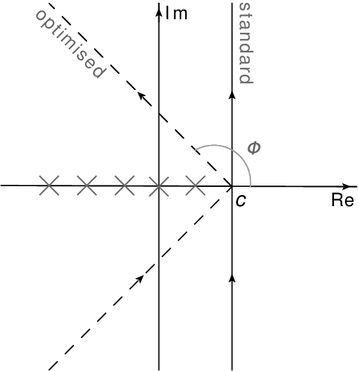
Refer to caption — Figure 2: Standard and optimised integration contours in the complex plane for the inverse Mellin transform. The two contours intersect the real axis at the point $c$ , and the optimised contour is bent by an angle $\phi>\pi/2$ with respect to the real axis. The crosses represent the poles of PDF parameterisation in Mellin space.

In DYTurbo, the Mellin moments of PDFs are evaluated numerically, by using Gauss-Legendre quadrature to calculate the integrals of Eq. (13). However these integrals can be evaluated numerically only for $\real(N)>0$ . As a consequence the integration contour of the inverse Mellin transform cannot be bent towards negative values of $\real(N)$ , and a standard contour along the straight line $[{c-i\infty},{c+i\infty}]$ is used (see Figure 2). This procedure results in a slower convergence of the integration in Eq. (12), for which about twice as many function evaluations are required, but it has the great advantage of allowing usage of PDFs with arbitrary parameterisation, without requiring knowledge of their functional form, and without requiring any time consuming evaluation of an approximation of PDFs in the form of Eq. (14). The integration over the $V$ -boson rapidity, $y$ , is factorised as follows. In the case of total cross sections, the values of the angular integrals in Eqs. (7) and (8) do not depend on $y$ . The only dependence on the rapidity in Eq. (12) is in the expression

\displaystyle x_{1}^{-N_{1}}x_{2}^{-N_{2}}=e^{-\ln(m/\sqrt{s})\,(N_{1}+N_{2})}e^{-y\,(N_{1}-N_{2})}\,,

(16)

and the integrals of Eq. (16) are evaluated analytically using the following relation:

\displaystyle\int_{y_{0}}^{y_{1}}\textrm{d}y\,e^{-y\,(N_{1}-N_{2})}=\frac{e^{-y_{1}(N_{1}-N_{2})}-e^{-y_{0}(N_{1}-N_{2})}}{N_{1}-N_{2}}\,,

(17)

where $y_{0}$ and $y_{1}$ are the lower and upper $y$ -bin boundaries. In the case $N_{1}=N_{2}$ , Eq. (17) further simplifies to $y_{1}-y_{0}$ . When the $y$ -bin boundaries are larger than the allowed kinematic range $|y|\leq y_{\textrm{max}}$ , with $y_{\textrm{max}}=\ln(\sqrt{s}/m)$ , Eq. (17) simplifies to $2\pi i\,\delta(N_{1}-N_{2})$ , and the double Mellin inversion is reduced to a single Mellin inversion Bozzi:2007pn by setting $N_{1}=N_{2}=N$ . In the case of fiducial cross sections, the values of $\theta_{0}$ and $\theta_{1}$ in Eq. (9) also depend on $y$ , and the integrals

\displaystyle\int_{y_{0}}^{y_{1}}\textrm{d}y\,e^{-y\,(N_{1}-N_{2})}\,\theta_{0,1}(y)\;,

(18)

are evaluated numerically for all pairs of $N_{1}$ and $N_{2}$ by means of Gauss-Legendre quadrature. The integration over the $V$ -boson transverse momentum, $q_{\mathrm{T}}$ , can be performed analytically in the case of the full-lepton phase space cross sections, since the expressions in Eqs. (7) and (8) do not depend on $q_{\mathrm{T}}$ , and the only term that depends on $q_{\mathrm{T}}$ is $J_{0}(bq_{\mathrm{T}})$ of Eq. (10). By using the relation $\int\textrm{d}x\,xJ_{0}(x)=xJ_{1}(x)$ , the integration over $q_{\mathrm{T}}$ in a bin of boundaries $q_{\mathrm{T}}^{0}$ and $q_{\mathrm{T}}^{1}$ can be evaluated as

\displaystyle\begin{split}&\int_{q_{\mathrm{T}}^{0}}^{q_{\mathrm{T}}^{1}}\textrm{d}q_{\mathrm{T}}\,2q_{\mathrm{T}}\,\mathcal{W}(q_{\mathrm{T}},m)=\\ \frac{m^{2}}{s}&\int_{0}^{\infty}{\textrm{d}b}\;\left[q_{\mathrm{T}}^{1}J_{1}(bq_{\mathrm{T}}^{1})-q_{\mathrm{T}}^{0}J_{1}(bq_{\mathrm{T}}^{0})\right]\;\mathcal{\tilde{W}}(b,m)\;.\end{split}

(19)

Similarly to Eq. (10), the integral of Eq. (19) is computed by means of a double-exponential formula for numerical integration, and by performing two separate integrations corresponding to the terms $J_{1}(bq_{\mathrm{T}}^{1})$ and $J_{1}(bq_{\mathrm{T}}^{0})$ . The information of the one-loop (two-loop) virtual correction to the LO subprocess is contained in the $\mathcal{H}^{V}$ function. In the computation of the fixed-order cross section of Eq. (4), the $\mathcal{H}^{V}$ function is evaluated in $x$ -space, i.e. without performing a Mellin transformation, and the convolution with PDFs is performed by integrating over the variables $z_{1,2}=e^{\pm\hat{y}}\,m/\sqrt{\hat{s}}$ . The corresponding integrals are calculated with Gauss–Legendre quadrature.

2.2 Asymptotic term and counter-term

The asymptotic term of Eq. (3) and the counter-term of Eq. (5) are computed using the function $\Sigma^{\textrm{V}}(q_{\mathrm{T}}/Q)$ , which embodies the singular behaviour of $\textrm{d}\sigma^{\textrm{f.o.}}$ in the limit $q_{\mathrm{T}}\to 0$ . In the finite-order case the counter-term contributes at $q_{\mathrm{T}}=0$ . Accordingly, the LO cross section is evaluated at $q_{\mathrm{T}}=0$ and the function $\Sigma^{\textrm{V}}(q_{\mathrm{T}}^{\prime}/Q)$ is integrated over the auxiliary variable $q_{\mathrm{T}}^{\prime}$ . At variance, in the resummed case the asymptotic term is a function of $q_{\mathrm{T}}$ , and the LO cross section is evaluated for nonzero values of $q_{\mathrm{T}}$ according to a given $q_{\mathrm{T}}$ -recoil prescription. As for the resummed term, the integration over the angular variables is factorised in the LO cross section by using Eqs. (7) and (8) or Eq. (9). The function $\Sigma^{\textrm{V}}(q_{\mathrm{T}}/Q)$ is evaluated in $x$ -space, i.e. without performing a Mellin transformation, and the convolution with PDFs is performed by integrating over the variables $z_{1,2}$ with Gauss–Legendre quadrature. In the case of full-lepton phase space cross sections, the $q_{\mathrm{T}}$ dependence of the asymptotic term and of the function $\Sigma^{\textrm{V}}(q_{\mathrm{T}}/Q)$ is fully embodied in a set of four functions $\tilde{I}_{n}(q_{\mathrm{T}}/Q)$ with $n=1,...,4$ Bozzi:2005wk. The integration over $q_{\mathrm{T}}$ of the asymptotic term is performed by integrating the $\tilde{I}_{n}(q_{\mathrm{T}}/Q)$ functions with Gauss–Legendre quadrature. In the case of fiducial cross sections, the values of $\theta_{0}$ and $\theta_{1}$ of Eq. (9) also depend on $q_{\mathrm{T}}$ , and the integrals

\displaystyle\int_{q_{\mathrm{T}}^{0}}^{q_{\mathrm{T}}^{1}}\textrm{d}q_{\mathrm{T}}\,2q_{\mathrm{T}}\,\tilde{I}_{n}(q_{\mathrm{T}}/Q)\,\theta_{i}(q_{\mathrm{T}})\;,\penalty\ \penalty\ \penalty\ \penalty\ \penalty\ \penalty\ i=0,1\;,

(20)

where $q_{\mathrm{T}}^{0}$ and $q_{\mathrm{T}}^{1}$ are the lower and upper $q_{\mathrm{T}}$ -bin boundaries, are evaluated numerically by means of Gauss–Legendre quadrature.

2.3 Finite-order term

The real-emission corrections are embodied in the (N)LO finite-order term of Eq. (1) and in the $V$ +jet term of Eq. (4) for the resummed and fixed-order predictions, respectively. Since DYTurbo provides results that are inclusive over final-state QCD radiation, the two terms are fully equivalent ³³ 3 Resummed predictions can be computed only inclusively with respect to final-state QCD radiation, whereas fixed-order predictions could be evaluated differentially.. Two independent calculations of this term are implemented. The first calculation, which is based on the code MCFM Campbell:2010ff, is fully differential with respect to the lepton angular variables and the final-state QCD radiation. The second calculation, which is inclusive over the lepton angles and the QCD radiation, implements the analytic results of Refs. Ellis:1981hk; Arnold:1988dp; Gonsalves:1989ar, and it relies in part on the code taken from DYqT Bozzi:2010xn. The MCFM implementation of the lowest-order term $\textrm{d}\sigma^{\textrm{V+jet}}_{\textrm{LO}}$ can be evaluated by using either the Vegas integration method or the numerical integration based on interpolating functions. The MCFM implementation of the next-order term $\textrm{d}\sigma^{\textrm{V+jet}}_{\textrm{NLO}}$ is the most complex part of the calculation, and it can be evaluated only with the Vegas algorithm. The reason is that this NLO calculation is based on the Catani–Seymour dipole subtraction scheme Catani:1996vz, in which for each point in the phase space where the real radiation is evaluated, a set of counter-term dipoles are computed corresponding to various different phase-space points. As in any local subtraction procedure, the resulting integrand presents discontinuities and it cannot be efficiently approximated by interpolating functions. The implementation of the analytic calculation of Refs. Ellis:1981hk; Arnold:1988dp; Gonsalves:1989ar yields the triple-differential production cross sections as a function of $q_{\mathrm{T}}$ , $m$ , and $y$ of the lepton pair, and it is used only for cross sections inclusive over the lepton decay, evaluated with numerical integration based on interpolating functions.

3 Tests of numerical precision

In order to validate the numerical precision of the resummed calculation, three closure tests are performed: the comparison of the fixed-order expansion of the resummed component (asymptotic term) and the finite-order term at small $q_{\mathrm{T}}$ , the comparison of the term $\mathcal{H}^{\textrm{V}}\times\textrm{d}\sigma^{\textrm{V}}_{\textrm{LO}}$ and the resummed component upon $q_{\mathrm{T}}$ integration, and comparisons of the integration methods available in DYTurbo, namely the Vegas algorithm and the multi-dimensional numerical integration based on interpolating functions, referred to as Quadrature integration in the plots. The numerical tests of this section are performed in full-lepton phase space, using the CT10nnlo set of parton density functions and with default values of the QCD scales and EW parameters. As discussed in Section 2, the function $\textrm{d}\sigma^{\textrm{asy}}$ embodies the singular behaviour of $\textrm{d}\sigma^{\textrm{f.o.}}$ when $q_{\mathrm{T}}\to 0$ , yielding the relation (see Eq. (4) of Ref. Bozzi:2005wk)

\displaystyle\lim_{Q_{\mathrm{T}}\to 0}\,\int_{0}^{Q_{\mathrm{T}}}\textrm{d}q_{\mathrm{T}}^{2}\left(\textrm{d}\sigma^{\textrm{\scriptsize f.o.}}-\textrm{d}\sigma^{\textrm{\scriptsize asy}}\right)=0\,,

(21)

or, equivalently,

\displaystyle\lim_{q_{\mathrm{T}}\to 0}\,q_{\mathrm{T}}\,\left(\textrm{d}\sigma^{\textrm{\scriptsize f.o.}}-\textrm{d}\sigma^{\textrm{\scriptsize asy}}\right)=0\,.

(22)

We note that $\textrm{d}\sigma^{\textrm{\scriptsize f.o.}}$ and $\textrm{d}\sigma^{\textrm{\scriptsize asy}}$ in Eq. (22) separately diverge proportionally to $q_{\mathrm{T}}^{-2}$ (modulo powers of $\log q_{\mathrm{T}}$ ) as $q_{\mathrm{T}}\to 0$ . Computing such a relation at small values of $Q_{\mathrm{T}}$ provides a stringent test of the numerical precision of the asymptotic and finite-order terms. The triple-differential cross sections $\textrm{d}\sigma^{\textrm{asy}}$ and $\textrm{d}\sigma^{\textrm{f.o.}}$ , as functions of $q_{\mathrm{T}}$ , $m$ and $y$ , are evaluated at the fixed values $y=0$ and $m=m_{V}$ , with $V=W,Z$ , for proton–proton collisions at $\sqrt{s}=13$ TeV. The result of the test is shown in Figure 3 for the NLL+NLO and NNLL+NNLO calculations. In all the cases, the relation of Eq. (22) is shown at values of $q_{\mathrm{T}}$ as low as $q_{\mathrm{T}}=0.01$ GeV.

Figure 3: Closure test of the relation

\textrm{d}\sigma^{\textrm{asy}}\sim\textrm{d}\sigma^{\textrm{f.o.}}

when

q_{\mathrm{T}}\to 0

for (a)

Z/\gamma^{*}

-boson, (b) positively-charged

W

-boson, and (c) negatively-charged

W

-boson production at

\sqrt{s}=13

TeV.

As a second closure test, the unitarity constraint of Eq. (6), which relates the $\mathcal{H}^{\textrm{V}}\times\textrm{d}\sigma^{\textrm{V}}_{\textrm{LO}}$ and $\textrm{d}\sigma^{\textrm{res}}$ terms, is tested. Computing such a relation provides a stringent test of the numerical precision of the procedure. The triple-differential cross sections $\textrm{d}\sigma^{\textrm{res}}$ as a function of $q_{\mathrm{T}}$ , $m$ , and $y$ are integrated in $q_{\mathrm{T}}$ from zero to infinity, and in the range of rapidity $|y|\leq y_{\textrm{max}}$ , and they are compared with the $\mathcal{H}^{\textrm{V}}\times\textrm{d}{\hat{\sigma}}^{\textrm{V}}_{\textrm{LO}}(0)$ double differential cross sections as a function of $m$ and $y$ , integrated in the same range of rapidity. The switching function $w(q_{\mathrm{T}},m)$ , which reduces the contribution of the resummed calculation in the large- $q_{\mathrm{T}}$ region, is not used in this test. Figure 4 shows the result of such a comparison at LO, NLO and NNLO for $Z/\gamma^{*}$ -boson production in proton–proton collisions at $\sqrt{s}=13$ TeV, for 180 equally-spaced bins of $m$ in the range $[20,200]$ GeV. In all cases the relation $\bigl(\int_{0}^{\infty}\textrm{d}q_{\mathrm{T}}^{2}\,\textrm{d}\sigma^{\textrm{res}}\bigr)/\bigl(\mathcal{H}^{\textrm{V}}\times\textrm{d}{\hat{\sigma}}^{\textrm{V}}_{\textrm{LO}}\bigr)=1$ is verified, with deviations from unity that are smaller than $10^{-6}$ . The terms $\mathcal{H}^{\textrm{V}}\times\textrm{d}\sigma^{\textrm{V}}_{\textrm{LO}}$ and $\textrm{d}\sigma^{\textrm{res}}$ are evaluated in $x$ -space and Mellin-space, respectively. Therefore, computing such a relation also provides a test of the numerical precision of the Mellin inverse transformation in Eq. (12). Similar level of agreement is observed by performing this closure test as a function of the rapidity.

Figure 4: Closure test of the relation

\int_{0}^{\infty}\textrm{d}q_{\mathrm{T}}^{2}\,\textrm{d}\sigma^{\textrm{res}}=\mathcal{H}^{\textrm{V}}\times\textrm{d}{\hat{\sigma}}^{\textrm{V}}_{\textrm{LO}}

for

Z/\gamma^{*}

-boson production at

\sqrt{s}=13

TeV, results at: (a) LO and LL, (b) NLO

{}^{\textrm{virt}}

and NLL, (c) NNLO

{}^{\textrm{virt}}

and NNLL. The labels NLO

{}^{\textrm{virt}}

(NNLO

{}^{\textrm{virt}}

) identify the contribution of the regularised virtual corrections up to one-loop (two-loop) order.

The results at NNLL+NNLO from DYTurbo using the numerical integration based on interpolating functions and the Vegas algorithm are compared for the $Z$ -boson differential cross section in proton–proton collisions at $\sqrt{s}=8$ TeV. The $Z$ -boson invariant mass range is required to be $80\penalty\ {\rm GeV}<m<100$ GeV. Ratios of these results are shown in Figure 5. The scatter in the central values of the points is at the permille level, except for the points at the very edges of the kinematic phase space, and for the finite-order term at high $q_{\mathrm{T}}$ where deviations of two permille are observed.

Figure 5: Ratio of full-lepton phase space differential cross sections at

\sqrt{s}=8

TeV as a function of

Z

-boson transverse momentum as evaluated with the Quadrature and Vegas integration methods of DYTurbo. From left to right: resummed component, asymptotic term, finite-order term, and total differential cross section.

4 Benchmark results

This section provides benchmark results of DYTurbo to DYRes at NNLL+NNLO for cross sections differential in $q_{\mathrm{T}}$ , and benchmark results of DYTurbo to DYRes and DYNNLO for fully-integrated fiducial cross sections at NNLL+NNLO and NNLO.

4.1 Benchmark of DYTurbo to DYRes differential results

Predictions at NNLL+NNLO for $Z$ -boson and $W$ -boson cross sections in proton–proton collisions at $\sqrt{s}=7$ TeV using the CT10nnlo set of parton density functions were evaluated with DYRes Catani:2015vma and compared to the corresponding predictions in DYTurbo. The $W$ -boson predictions are in the full-lepton phase space, whereas the $Z$ -boson predictions are fiducial, and match the kinematic definition of Ref. Aad:2014xaa. Careful attention is paid to exactly match in DYTurbo the settings used to produce the DYRes predictions, such as QCD scales choice, EW scheme and input parameters, switching function at high $q_{\mathrm{T}}$ , $q_{\mathrm{T}}$ -recoil prescription, and the prescription for avoiding the Landau pole in $b$ -space. All these parameters are set to the default values of DYRes. Figures 6 and 7 show the comparisons to DYRes of DYTurbo results for the $Z$ -boson and positively-charged $W$ -boson production cross sections. The $Z$ -boson fiducial phase space is defined by the lepton transverse momentum $p_{\mathrm{T}}^{\ell}>20$ GeV, the lepton pseudorapidity $|\eta_{\ell}|<2.4$ , and invariant mass of the lepton pair in the range $66\penalty\ {\rm GeV}<m<116$ GeV. All comparisons of predictions for the resummed term are validated at the better than 1% level while the comparison of the sum of the asymptotic and finite-order terms are validated at the $\sim$ 2% level for $q_{\mathrm{T}}$ above 40 GeV. In particular, the positively-charged $W$ -boson predictions show well that the sum of the asymptotic and finite-order terms converges to zero at low $q_{\mathrm{T}}$ , as expected (it is also consistent with zero for the $Z$ -boson predictions, within the Vegas uncertainties, which are highly correlated bin-to-bin).

Figure 6: Comparison of differential fiducial cross sections computed with DYRes and DYTurbo at

\sqrt{s}=7

TeV as a function of the

Z

-boson transverse momentum. The

Z

-boson fiducial phase space is defined by the lepton transverse momentum

p_{\mathrm{T}}^{\ell}>20

GeV, the lepton pseudorapidity

|\eta_{\ell}|<2.4

, and the invariant mass of the lepton pair

66\penalty\ {\rm GeV}<m<116

GeV. (a) Comparison of resummed component between DYRes and DYTurbo with Vegas integration. (b) Comparison of resummed component between DYRes and DYTurbo with Quadrature integration. (c) Comparison of the sum of asymptotic and finite-order terms between DYRes and DYTurbo with Vegas integration. The top panels show absolute cross sections, and the bottom panels show ratios of DYTurbo to DYRes results.

Figure 7: Comparison of full-lepton phase space differential cross sections computed with DYRes and DYTurbo (Quadrature integration method) at

\sqrt{s}=7

TeV as a function of the transverse momentum of the positively-charged

W

-boson: (a) resummed component, (b) sum of asymptotic and finite-order terms. The top panels show absolute cross sections, and the bottom panels show ratios of DYTurbo to DYRes results.

The DYTurbo and DYRes results are compared in Figure 8 after summing all terms. Also in this case good agreement is observed between the two codes, within the numerical uncertainty of the Vegas integration.

Figure 8: Comparison of DYRes and DYTurbo cross sections at

\sqrt{s}=7

TeV as a function of the boson transverse momentum for full-lepton phase space

W^{+}

and

W^{-}

production, and fiducial

Z

-boson production.

4.2 Benchmark of fully-integrated cross-section results

Benchmark results for fully-integrated fiducial cross section at NNLL+NNLO from DYRes Catani:2015vma and at NNLO from DYNNLO Catani:2009sm are shown in Table 1 and compared with the corresponding results calculated with DYTurbo ⁴⁴ 4 The NNLO results in Table 1 are obtained with a minimum value of $r=q_{\mathrm{T}}/m$ fixed to $r_{\textrm{cut}}=0.002$ and their corresponding numerical uncertainties do not include the systematic uncertainty from the $r_{\textrm{cut}}\to 0$ extrapolation. A more accurate NNLO result and an estimate of such uncertainty can be obtained by evaluating the cross section at different values of $r_{\textrm{cut}}$ and carrying out the limit $r_{\textrm{cut}}\to 0$ Grazzini:2017mhc.. The predictions are evaluated for proton–proton collisions at the centre–of–mass energy $\sqrt{s}=8$ TeV, and according to the fiducial definition and QCD and EW settings of Ref. Alioli:2016fum. The $Z$ - and $W$ -boson fiducial phase space is defined by the charged lepton and neutrino transverse momentum $p_{\mathrm{T}}^{\ell,\nu}>25$ GeV, the charged lepton pseudorapidity $|\eta_{\ell}|<2.5$ , and invariant mass of the lepton pair larger than $50$ GeV for $Z$ -boson production and larger than $1$ GeV for $W$ -boson production. The results for DYNNLO shown in the table are taken from Table 12 of Ref. Alioli:2016fum. The results of DYTurbo are in agreement with the results of the other programs considered in Ref. Alioli:2016fum. Differences as large as 1% are observed between the NNLO and the NNLL+NNLO results, which are mostly due to recoil effects in the lepton kinematics (the unitarity constraint of Eq. (6) between fixed-order and resummed calculations does not apply in the presence of lepton kinematic cuts). An additional source of difference between the NNLO and the NNLL+NNLO results is the inclusion of the switching function $w(q_{\mathrm{T}},m)$ , which affects the cross sections at the per mille level.

Table 1: Comparison of NNLO and NNLO+NNLL cross-section results at

\sqrt{s}=8

TeV. The results for DYNNLO are taken from Ref. Alioli:2016fum.

Program	DYNNLO	DYTurbo	DYRes	DYTurbo
Order	NNLO	NNLO	NNLO+NNLL	NNLO+NNLL
$\sigma(pp\rightarrow W^{+}\rightarrow l^{+}\nu$ ) [pb]	$3191\pm 7$	$3176\pm 3$	$3149\pm 8$	$3155\pm 3$
$\sigma(pp\rightarrow W^{-}\rightarrow l^{-}\nu$ ) [pb]	$2243\pm 6$	$2234\pm 2$	$2214\pm 4$	$2213\pm 2$
$\sigma(pp\rightarrow Z/\gamma^{*}\rightarrow l^{+}l^{-}$ ) [pb]	$502.4\pm 0.4$	$502.8\pm 0.5$	$500.7\pm 0.9$	$500.5\pm 0.6$

5 Time performance

In this section various tests of time performance are discussed. The computation time requested to calculate cross-section predictions for DYTurbo and DYRes is compared and used to assess the performance improvement of DYTurbo. The amount of time required to perform a calculation as a function of threads provides a test of the scaling behaviour of the multi-threading implementation. The time-performance tests are run on a server mounting two AMD Opteron 6344 CPUs with 12 cores each. The fully-integrated fiducial cross section of $Z$ -boson production, as defined for the results shown in Table 1, is computed with DYRes and DYTurbo at NNLL+NNLO. The DYRes calculation took 40 hours for an uncertainty of 0.4 DYTurbo took 8 hours, yielding a factor of 5 in the improvement of the time performance. Figure 9 shows the speedup factors for cross-section calculations as a function of the number of threads, where the speedup is defined as the ratio of elapsed time of the multi-threaded calculation divided by the reference elapsed time of the one-thread calculation. Assuming that the one-thread calculation has a parallelisable time fraction and a non-parallelisable time fraction, and the multithreading process has an overhead time proportional to the number of threads $N$ , the speedup curve can be parameterised as $(1+s)/(1/N+s+o\cdot N)$ . where $s$ is the ratio between non-parallelisable and parallelisable times, and $o$ is the overhead time per thread. The measured speedup factors are well described by this model, with overhead times compatible with zero, and with fractions of non-parallelisable time which are smaller when the target precision is higher. Indeed most of the non-parallelisable time is spent in the program initialisation, which becomes negligible for long runs with high target precision.

Figure 9: Computing time as a function of the number of threads for

Z

-boson production at

\sqrt{s}=8

TeV with different target precision: (a) NNLO results with the Vegas integration method, and (b) NNLL+NNLO results with the Quadrature integration method.

We conclude this section reporting typical running times for fast and numerically precise DYTurbo predictions with the numerical integration based on interpolating functions. Figure 10 shows NLL+NLO and NNLL+NNLO predictions for the $Z$ -boson production at 13 TeV in full-lepton phase space, integrated in the range of invariant mass $[66,116]$ GeV and in the range of rapidity $|y|\leq y_{\textrm{max}}\sim 5.3$ . The predictions are computed in 100 equally-spaced $q_{\mathrm{T}}$ bins from zero to 25 GeV. The predictions are evaluated with a target in the relative numerical uncertainty of $10^{-4}$ for each term, and using simultaneously 20 parallel threads. The computation time required to perform the full calculation is 4 min at NLL+NLO and 3.4 hours at NNLL+NNLO. The computation of the resummed component required 6 seconds at NLL+NLO and 10 seconds at NNLL+ NNLO, the computation of the asymptotic term required 0.2 seconds at NLL+NLO and 0.7 seconds at NNLL+NNLO, the computation of the finite-order term required 4 min at NLL+NLO and 3.4 hours at NNLL+ NNLO. In these examples, as in all other time-performance tests, the great majority of the computation time is spent to evaluate the finite-order term. For applications as PDF fits, where very fast predictions are required, this part of the calculation could be computed by using APPLGRID Carli:2010rw.

Figure 10: Example of predictions at NLL+NLO and NNLL+NNLO accuracy for

Z

-boson production at

\sqrt{s}=13

TeV.

6 Conclusions

The DYTurbo program provides fast and numerical precise predictions of Drell–Yan processes, through a new implementation of the DYqT, DYRes and DYNNLO numerical codes. The cross-section predictions include the calculation of the QCD transverse-momentum resummation up to next-to-next-to-leading logarithmic accuracy combined with the fixed-order results at next-to-next-to-leading order ( $\mathcal{O}(\alpha_{\mathrm{S}}^{2})$ ). They also include the full kinematical dependence of the decaying lepton pair with the corresponding spin correlations and the finite-width effects. The enhancement in performance over previous programs is achieved by code optimisation, by factorising the cross section into production and decay variables, and with the usage of numerical integration based on interpolating functions. The resulting cross-section predictions are in agreement with the results of the original programs. The great reduction of computing time for performing cross-sections calculation opens new possibilities for the usage of Drell–Yan processes for PDF fits, for the extraction of fundamental parameters of the SM, such as the mass of the $W$ boson and the weak-mixing angle, and for the estimation of background processes in searches for physics beyond the SM.

Acknowledgements.

We thank Sven Moch for fruitful discussions on Mellin transformations. M. S. acknowledges support from the Volkswagen Foundation and the German Research Foundation (DFG). G. B. acknowledges support from the European Research Council (ERC) under the European Union’s Horizon 2020 research and innovation program (grant agreement No. 647981, 3DSPIN).

References

(1) S. D. Drell and T.-M. Yan, “Massive lepton-pair production in hadron-hadron collisions at high energies,” Phys. Rev. Lett. 25 (Sep, 1970) 902–902.
(2) J. H. Christenson, G. S. Hicks, L. M. Lederman, P. J. Limon, B. G. Pope, and E. Zavattini, “Observation of massive muon pairs in hadron collisions,” Phys. Rev. Lett. 25 (Nov, 1970) 1523–1526.
(3) L. Evans and P. Bryant, “LHC Machine,” JINST 3 no. 08, (2008) S08001.
(4) CMS Collaboration, “Measurement of the differential cross section and charge asymmetry for inclusive $\mathrm{p}\mathrm{p}\rightarrow\mathrm{W}^{\pm}+X$ production at ${\sqrt{s}}=8$ TeV,” Eur. Phys. J. C 76 no. 8, (2016) 469, arXiv:1603.01803 [hep-ex].
(5) ATLAS Collaboration, “Precision measurement and interpretation of inclusive $W^{+}$ , $W^{-}$ and $Z/\gamma^{*}$ production cross sections with the ATLAS detector,” Eur. Phys. J. C 77 no. 6, (2017) 367, arXiv:1612.03016 [hep-ex].
(6) ATLAS Collaboration, “Measurement of the $W$ -boson mass in pp collisions at $\sqrt{s}=7$ TeV with the ATLAS detector,” Eur. Phys. J. C 78 no. 2, (2018) 110, arXiv:1701.07240 [hep-ex].
(7) ATLAS Collaboration, “Measurement of the forward-backward asymmetry of electron and muon pair-production in $pp$ collisions at $\sqrt{s}$ = 7 TeV with the ATLAS detector,” JHEP 09 (2015) 049, arXiv:1503.03709 [hep-ex].
(8) CMS Collaboration, “Measurement of the weak mixing angle with the Drell-Yan process in proton-proton collisions at the LHC,” Phys. Rev. D 84 (2011) 112002, arXiv:1110.2682 [hep-ex].
(9) S. Camarda, J. Cuth, and M. Schott, “Determination of the muonic branching ratio of the W boson and its total width via cross-section measurements at the Tevatron and LHC,” Eur. Phys. J. C 76 no. 11, (2016) 613, arXiv:1607.05084 [hep-ex].
(10) CMS Collaboration, “Search for narrow resonances in dilepton mass spectra in proton-proton collisions at $\sqrt{s}$ = 13 TeV and combination with 8 TeV data,” Phys. Lett. B 768 (2017) 57–80, arXiv:1609.05391 [hep-ex].
(11) CMS Collaboration, “Search for heavy gauge W’ boson in events with an energetic lepton and large missing transverse momentum at $\sqrt{s}=$ 13 TeV,” Phys. Lett. B 770 (2017) 278–301, arXiv:1612.09274 [hep-ex].
(12) ATLAS Collaboration, “Search for high-mass new phenomena in the dilepton final state using proton-proton collisions at $\sqrt{s}=13$ TeV with the ATLAS detector,” Phys. Lett. B 761 (2016) 372–392, arXiv:1607.03669 [hep-ex].
(13) ATLAS Collaboration, “Search for new resonances in events with one lepton and missing transverse momentum in $pp$ collisions at $\sqrt{s}=13$ TeV with the ATLAS detector,” Phys. Lett. B 762 (2016) 334–352, arXiv:1606.03977 [hep-ex].
(14) R. Hamberg, W. L. van Neerven, and T. Matsuura, “A complete calculation of the order $\alpha_{s}^{2}$ correction to the Drell-Yan $K$ factor,” Nucl. Phys. B 359 (1991) 343–405. [Erratum: Nucl. Phys.B644,403(2002)].
(15) R. V. Harlander and W. B. Kilgore, “Next-to-next-to-leading order Higgs production at hadron colliders,” Phys. Rev. Lett. 88 (2002) 201801, arXiv:hep-ph/0201206 [hep-ph].
(16) C. Anastasiou, L. J. Dixon, K. Melnikov, and F. Petriello, “High precision QCD at hadron colliders: Electroweak gauge boson rapidity distributions at NNLO,” Phys. Rev. D 69 (2004) 094008, arXiv:hep-ph/0312266 [hep-ph].
(17) K. Melnikov and F. Petriello, “The $W$ boson production cross section at the LHC through $O(\alpha^{2}_{s})$ ,” Phys. Rev. Lett. 96 (2006) 231803, arXiv:hep-ph/0603182 [hep-ph].
(18) K. Melnikov and F. Petriello, “Electroweak gauge boson production at hadron colliders through O( $\alpha_{s}^{2}$ ),” Phys. Rev. D 74 (2006) 114017, arXiv:hep-ph/0609070 [hep-ph].
(19) S. Catani, L. Cieri, G. Ferrera, D. de Florian, and M. Grazzini, “Vector boson production at hadron colliders: a fully exclusive QCD calculation at NNLO,” Phys. Rev. Lett. 103 (2009) 082001, arXiv:0903.2120 [hep-ph].
(20) S. Catani, G. Ferrera, and M. Grazzini, “W Boson Production at Hadron Colliders: The Lepton Charge Asymmetry in NNLO QCD,” JHEP 05 (2010) 006, arXiv:1002.3115 [hep-ph].
(21) R. Boughezal, C. Focke, X. Liu, and F. Petriello, “ $W$ -boson production in association with a jet at next-to-next-to-leading order in perturbative QCD,” Phys. Rev. Lett. 115 no. 6, (2015) 062002, arXiv:1504.02131 [hep-ph].
(22) A. Gehrmann-De Ridder, T. Gehrmann, E. W. N. Glover, A. Huss, and T. A. Morgan, “Precise QCD predictions for the production of a Z boson in association with a hadronic jet,” Phys. Rev. Lett. 117 no. 2, (2016) 022001, arXiv:1507.02850 [hep-ph].
(23) R. Boughezal, J. M. Campbell, R. K. Ellis, C. Focke, W. T. Giele, X. Liu, and F. Petriello, “Z-boson production in association with a jet at next-to-next-to-leading order in perturbative QCD,” Phys. Rev. Lett. 116 no. 15, (2016) 152001, arXiv:1512.01291 [hep-ph].
(24) R. Boughezal, X. Liu, and F. Petriello, “W-boson plus jet differential distributions at NNLO in QCD,” Phys. Rev. D 94 no. 11, (2016) 113009, arXiv:1602.06965 [hep-ph].
(25) A. Gehrmann-De Ridder, T. Gehrmann, E. W. N. Glover, A. Huss, and D. M. Walker, “Next-to-Next-to-Leading-Order QCD Corrections to the Transverse Momentum Distribution of Weak Gauge Bosons,” Phys. Rev. Lett. 120 no. 12, (2018) 122001, arXiv:1712.07543 [hep-ph].
(26) Y. L. Dokshitzer, D. Diakonov, and S. I. Troian, “On the Transverse Momentum Distribution of Massive Lepton Pairs,” Phys. Lett. B 79 (1978) 269–272.
(27) G. Parisi and R. Petronzio, “Small Transverse Momentum Distributions in Hard Processes,” Nucl. Phys. B 154 (1979) 427–440.
(28) J. C. Collins, D. E. Soper, and G. F. Sterman, “Transverse Momentum Distribution in Drell-Yan Pair and W and Z Boson Production,” Nucl. Phys. B 250 (1985) 199–224.
(29) S. Catani, L. Cieri, D. de Florian, G. Ferrera, and M. Grazzini, “Universality of transverse-momentum resummation and hard factors at the NNLO,” Nucl. Phys. B 881 (2014) 414–443, arXiv:1311.1654 [hep-ph].
(30) C. Balazs and C. P. Yuan, “Soft gluon effects on lepton pairs at hadron colliders,” Phys. Rev. D 56 (1997) 5558–5583, arXiv:hep-ph/9704258 [hep-ph].
(31) R. K. Ellis, D. A. Ross, and S. Veseli, “Vector boson production in hadronic collisions,” Nucl. Phys. B 503 (1997) 309–338, arXiv:hep-ph/9704239 [hep-ph].
(32) R. K. Ellis and S. Veseli, “ $W$ and $Z$ transverse momentum distributions: Resummation in $q_{T}$ space,” Nucl. Phys. B 511 (1998) 649–669, arXiv:hep-ph/9706526 [hep-ph].
(33) G. Bozzi, S. Catani, G. Ferrera, D. de Florian, and M. Grazzini, “Production of Drell-Yan lepton pairs in hadron collisions: Transverse-momentum resummation at next-to-next-to-leading logarithmic accuracy,” Phys. Lett. B 696 (2011) 207–213, arXiv:1007.2351 [hep-ph].
(34) A. Banfi, M. Dasgupta, S. Marzani, and L. Tomlinson, “Predictions for Drell-Yan $\phi^{*}$ and $Q_{T}$ observables at the LHC,” Phys. Lett. B715 (2012) 152–156, arXiv:1205.4760 [hep-ph].
(35) M. Guzzi, P. M. Nadolsky, and B. Wang, “Nonperturbative contributions to a resummed leptonic angular distribution in inclusive neutral vector boson production,” Phys. Rev. D 90 no. 1, (2014) 014030, arXiv:1309.1393 [hep-ph].
(36) S. Catani, D. de Florian, G. Ferrera, and M. Grazzini, “Vector boson production at hadron colliders: transverse-momentum resummation and leptonic decay,” JHEP 12 (2015) 047, arXiv:1507.06937 [hep-ph].
(37) W. Bizoń, X. Chen, A. Gehrmann-De Ridder, T. Gehrmann, N. Glover, A. Huss, P. F. Monni, E. Re, L. Rottoli, and P. Torrielli, “Fiducial distributions in Higgs and Drell-Yan production at N³LL+NNLO,” JHEP 12 (2018) 132, arXiv:1805.05916 [hep-ph].
(38) W. Bizon, A. Gehrmann-De Ridder, T. Gehrmann, N. Glover, A. Huss, P. F. Monni, E. Re, L. Rottoli, and D. M. Walker, “The transverse momentum spectrum of weak gauge bosons at N³LL $+$ NNLO,” arXiv:1905.05171 [hep-ph].
(39) T. Becher and M. Neubert, “Drell-Yan Production at Small $q_{T}$ , Transverse Parton Distributions and the Collinear Anomaly,” Eur. Phys. J. C 71 (2011) 1665, arXiv:1007.4005 [hep-ph].
(40) T. Becher, M. Neubert, and D. Wilhelm, “Electroweak Gauge-Boson Production at Small $q_{T}$ : Infrared Safety from the Collinear Anomaly,” JHEP 02 (2012) 124, arXiv:1109.6027 [hep-ph].
(41) J.-Y. Chiu, A. Jain, D. Neill, and I. Z. Rothstein, “A Formalism for the Systematic Treatment of Rapidity Logarithms in Quantum Field Theory,” JHEP 05 (2012) 084, arXiv:1202.0814 [hep-ph].
(42) M. A. Ebert and F. J. Tackmann, “Resummation of Transverse Momentum Distributions in Distribution Space,” JHEP 02 (2017) 110, arXiv:1611.08610 [hep-ph].
(43) T. Becher and M. Hager, “Event-Based Transverse Momentum Resummation,” arXiv:1904.08325 [hep-ph].
(44) J. Collins, “Foundations of perturbative QCD,” Camb. Monogr. Part. Phys. Nucl. Phys. Cosmol. 32 (2011) 1–624.
(45) M. G. Echevarria, A. Idilbi, and I. Scimemi, “Factorization Theorem For Drell-Yan At Low $q_{T}$ And Transverse Momentum Distributions On-The-Light-Cone,” JHEP 07 (2012) 002, arXiv:1111.4996 [hep-ph].
(46) J. C. Collins and T. C. Rogers, “Equality of Two Definitions for Transverse Momentum Dependent Parton Distribution Functions,” Phys. Rev. D 87 no. 3, (2013) 034018, arXiv:1210.2100 [hep-ph].
(47) J. Collins and T. Rogers, “Understanding the large-distance behavior of transverse-momentum-dependent parton densities and the Collins-Soper evolution kernel,” Phys. Rev. D 91 no. 7, (2015) 074020, arXiv:1412.3820 [hep-ph].
(48) I. Scimemi and A. Vladimirov, “Analysis of vector boson production within TMD factorization,” Eur. Phys. J. C 78 no. 2, (2018) 89, arXiv:1706.01473 [hep-ph].
(49) V. Bertone, I. Scimemi, and A. Vladimirov, “Extraction of unpolarized quark transverse momentum dependent parton distributions from Drell-Yan/Z-boson production,” JHEP 06 (2019) 028, arXiv:1902.08474 [hep-ph].
(50) A. Bacchetta, G. Bozzi, M. Lambertsen, F. Piacenza, J. Steiglechner, and W. Vogelsang, “Difficulties in the description of Drell-Yan processes at moderate invariant mass and high transverse momentum,” Phys. Rev. D 100 no. 1, (2019) 014018, arXiv:1901.06916 [hep-ph].
(51) A. Bacchetta, G. Bozzi, M. Radici, M. Ritzmann, and A. Signori, “Effect of Flavor-Dependent Partonic Transverse Momentum on the Determination of the $W$ Boson Mass in Hadronic Collisions,” Phys. Lett. B788 (2019) 542–545, arXiv:1807.02101 [hep-ph].
(52) G. Bozzi and A. Signori, “Nonperturbative Uncertainties on the Transverse Momentum Distribution of Electroweak Bosons and on the Determination of the Boson Mass at the LHC,” Adv. High Energy Phys. 2019 (2019) 2526897, arXiv:1901.01162 [hep-ph].
(53) S. Dittmaier and M. Krämer, “Electroweak radiative corrections to W boson production at hadron colliders,” Phys. Rev. D 65 (2002) 073007, arXiv:hep-ph/0109062 [hep-ph].
(54) U. Baur and D. Wackeroth, “Electroweak radiative corrections to $p\bar{p}\to W^{\pm}\to\ell^{\pm}\nu$ beyond the pole approximation,” Phys. Rev. D 70 (2004) 073015, arXiv:hep-ph/0405191 [hep-ph].
(55) V. A. Zykunov, “Radiative corrections to the Drell-Yan process at large dilepton invariant masses,” Phys. Atom. Nucl. 69 (2006) 1522. [Yad. Fiz.69,1557(2006)].
(56) A. Arbuzov, D. Bardin, S. Bondarenko, P. Christova, L. Kalinovskaya, G. Nanava, and R. Sadykov, “One-loop corrections to the Drell-Yan process in SANC. I. The Charged current case,” Eur. Phys. J. C 46 (2006) 407–412, arXiv:hep-ph/0506110 [hep-ph]. [Erratum: Eur. Phys. J.C50,505(2007)].
(57) C. M. Carloni Calame, G. Montagna, O. Nicrosini, and A. Vicini, “Precision electroweak calculation of the charged current Drell-Yan process,” JHEP 12 (2006) 016, arXiv:hep-ph/0609170 [hep-ph].
(58) U. Baur, O. Brein, W. Hollik, C. Schappacher, and D. Wackeroth, “Electroweak radiative corrections to neutral current Drell-Yan processes at hadron colliders,” Phys. Rev. D 65 (2002) 033007, arXiv:hep-ph/0108274 [hep-ph].
(59) V. A. Zykunov, “Weak radiative corrections to Drell-Yan process for large invariant mass of di-lepton pair,” Phys. Rev. D 75 (2007) 073019, arXiv:hep-ph/0509315 [hep-ph].
(60) C. M. Carloni Calame, G. Montagna, O. Nicrosini, and A. Vicini, “Precision electroweak calculation of the production of a high transverse-momentum lepton pair at hadron colliders,” JHEP 10 (2007) 109, arXiv:0710.1722 [hep-ph].
(61) A. Arbuzov, D. Bardin, S. Bondarenko, P. Christova, L. Kalinovskaya, G. Nanava, and R. Sadykov, “One-loop corrections to the Drell–Yan process in SANC. (II). The Neutral current case,” Eur. Phys. J. C 54 (2008) 451–460, arXiv:0711.0625 [hep-ph].
(62) A. Kotikov, J. H. Kuhn, and O. Veretin, “Two-Loop Formfactors in Theories with Mass Gap and Z-Boson Production,” Nucl. Phys. B 788 (2008) 47–62, arXiv:hep-ph/0703013 [HEP-PH].
(63) W. B. Kilgore and C. Sturm, “Two-Loop Virtual Corrections to Drell-Yan Production at order $\alpha_{s}\alpha^{3}$ ,” Phys. Rev. D 85 (2012) 033005, arXiv:1107.4798 [hep-ph].
(64) S. Dittmaier, A. Huss, and C. Schwinn, “Mixed QCD-electroweak O( $\alpha_{s}\alpha$ ) corrections to Drell-Yan processes in the resonance region: pole approximation and non-factorizable corrections,” Nucl. Phys. B 885 (2014) 318–372, arXiv:1403.3216 [hep-ph].
(65) R. Bonciani, F. Buccioni, R. Mondini, and A. Vicini, “Double-real corrections at $\mathcal{O}(\alpha\alpha_{s})$ to single gauge boson production,” Eur. Phys. J. C 77 no. 3, (2017) 187, arXiv:1611.00645 [hep-ph].
(66) L. Cieri, G. Ferrera, and G. F. R. Sborlini, “Combining QED and QCD transverse-momentum resummation for Z boson production at hadron colliders,” JHEP 08 (2018) 165, arXiv:1805.11948 [hep-ph].
(67) D. de Florian, M. Der, and I. Fabre, “QCD $\oplus$ QED NNLO corrections to Drell Yan production,” Phys. Rev. D 98 no. 9, (2018) 094008, arXiv:1805.12214 [hep-ph].
(68) M. Delto, M. Jaquier, K. Melnikov, and R. Röntsch, “Mixed QCD $\otimes$ QED corrections to on-shell $Z$ boson production at the LHC,” arXiv:1909.08428 [hep-ph].
(69) S. Catani, D. de Florian, and M. Grazzini, “Universality of nonleading logarithmic contributions in transverse momentum distributions,” Nucl. Phys. B 596 (2001) 299–312, arXiv:hep-ph/0008184 [hep-ph].
(70) G. Bozzi, S. Catani, D. de Florian, and M. Grazzini, “Transverse-momentum resummation and the spectrum of the Higgs boson at the LHC,” Nucl. Phys. B 737 (2006) 73–120, arXiv:hep-ph/0508068 [hep-ph].
(71) G. Bozzi, S. Catani, D. de Florian, and M. Grazzini, “Higgs boson production at the LHC: Transverse-momentum resummation and rapidity dependence,” Nucl. Phys. B 791 (2008) 1–19, arXiv:0705.3887 [hep-ph].
(72) R. K. Ellis, G. Martinelli, and R. Petronzio, “Lepton Pair Production at Large Transverse Momentum in Second Order QCD,” Nucl. Phys. B 211 (1983) 106–138.
(73) P. B. Arnold and M. H. Reno, “The Complete Computation of High $\textit{p}_{T}$ W and Z Production in 2nd Order QCD,” Nucl. Phys. B 319 (1989) 37–71. [Erratum: Nucl. Phys.B330,284(1990)].
(74) R. J. Gonsalves, J. Pawlowski, and C.-F. Wai, “QCD Radiative Corrections to Electroweak Boson Production at Large Transverse Momentum in Hadron Collisions,” Phys. Rev. D 40 (1989) 2245.
(75) J. M. Campbell and R. K. Ellis, “MCFM for the Tevatron and the LHC,” Nucl. Phys. Proc. Suppl. 205-206 (2010) 10–15, arXiv:1007.3492 [hep-ph].
(76) T. Hahn, “Concurrent Cuba,” J. Phys. Conf. Ser. 608 no. 1, (2015) 012066, arXiv:1408.6373 [physics.comp-ph].
(77) R. Brun and F. Rademakers, “ROOT: An object oriented data analysis framework,” Nucl. Instrum. Meth. A 389 (1997) 81–86.
(78) ATLAS Collaboration, “Measurements of top-quark pair to $Z$ -boson cross-section ratios at $\sqrt{s}=13,8,7$ TeV with the ATLAS detector,” JHEP 02 (2017) 117, arXiv:1612.03636 [hep-ex].
(79) ATLAS Collaboration, “Measurement of the effective leptonic weak mixing angle using electron and muon pairs from $Z$ -boson decay in the ATLAS experiment at $\sqrt{s}=8$ TeV,” Tech. Rep. ATLAS-CONF-2018-037, CERN, Geneva, Jul, 2018. http://cds.cern.ch/record/2630340.
(80) S. Camarda et al., “DYTurbo.” https://dyturbo.hepforge.org/.
(81) S. Catani and M. Grazzini, “An NNLO subtraction formalism in hadron collisions and its application to Higgs boson production at the LHC,” Phys. Rev. Lett. 98 (2007) 222002, arXiv:hep-ph/0703012 [hep-ph].
(82) G. P. Lepage, “A new algorithm for adaptive multidimensional integration,” Journal of Computational Physics 27 no. 2, (1978) 192 – 203.
(83) T. Hahn, “CUBA: A Library for multidimensional numerical integration,” Comput. Phys. Commun. 168 (2005) 78–95, arXiv:hep-ph/0404043 [hep-ph].
(84) S. Elhay and J. Kautsky, “Algorithm 655: Iqpack: Fortran subroutines for the weights of interpolatory quadratures,” ACM Trans. Math. Softw. 13 no. 4, (Dec., 1987) 399–415.
(85) J. Burkardt, “Sandia rules,” 2011. https://people.sc.fsu.edu/˜jburkardt/cpp_src/sandia_rules/sandia_rules.html.
(86) A. Genz and A. Malik, “Remarks on algorithm 006: An adaptive algorithm for numerical integration over an n-dimensional rectangular region,” Journal of Computational and Applied Mathematics 6 no. 4, (1980) 295 – 302.
(87) J. Berntsen, T. O. Espelid, and A. Genz, “An adaptive algorithm for the approximate calculation of multiple integrals,” ACM Trans. Math. Softw. 17 no. 4, (Dec., 1991) 437–451.
(88) S. Johnson, “Cubature,” 2005–2013. https://github.com/stevengj/cubature.
(89) J. Gao, M. Guzzi, J. Huston, H.-L. Lai, Z. Li, P. Nadolsky, J. Pumplin, D. Stump, and C. P. Yuan, “CT10 next-to-next-to-leading order global analysis of QCD,” Phys. Rev. D 89 no. 3, (2014) 033009, arXiv:1302.6246 [hep-ph].
(90) T. Ooura and M. Mori, “A robust double exponential formula for fourier-type integrals,” Journal of Computational and Applied Mathematics 112 no. 1, (1999) 229 – 241.
(91) T. Ooura and M. Mori, “The double exponential formula for oscillatory functions over the half infinite interval,” Journal of Computational and Applied Mathematics 38 no. 1, (1991) 353 – 360.
(92) T. Hidetosi and M. Masatake, “Double exponential formulas for numerical integration,” Publ. Res. Inst. Math. Sci. 9 (1973) 721–741.
(93) J. Blumlein and S. Kurth, “Harmonic sums and Mellin transforms up to two loop order,” Phys. Rev. D 60 (1999) 014018, arXiv:hep-ph/9810241.
(94) J. Blumlein, “Analytic continuation of Mellin transforms up to two loop order,” Comput. Phys. Commun. 133 (2000) 76–104, arXiv:hep-ph/0003100 [hep-ph].
(95) A. Vogt, “Efficient evolution of unpolarized and polarized parton distributions with QCD-PEGASUS,” Comput. Phys. Commun. 170 (2005) 65–92, arXiv:hep-ph/0408244 [hep-ph].
(96) M. Stratmann and W. Vogelsang, “Towards a global analysis of polarized parton distributions,” Phys. Rev. D 64 (2001) 114007.
(97) S. Catani and M. H. Seymour, “A General algorithm for calculating jet cross-sections in NLO QCD,” Nucl. Phys. B 485 (1997) 291–419, arXiv:hep-ph/9605323 [hep-ph]. [Erratum: Nucl. Phys. B 510,503(1998)].
(98) ATLAS Collaboration, “Measurement of the $Z/\gamma^{*}$ boson transverse momentum distribution in $pp$ collisions at $\sqrt{s}$ = 7 TeV with the ATLAS detector,” JHEP 09 (2014) 145, arXiv:1406.3660 [hep-ex].
(99) M. Grazzini, S. Kallweit, and M. Wiesemann, “Fully differential NNLO computations with MATRIX,” Eur. Phys. J. C 78 no. 7, (2018) 537, arXiv:1711.06631 [hep-ph].
(100) S. Alioli et al., “Precision studies of observables in $pp\rightarrow W\rightarrow l\nu_{l}$ and $pp\rightarrow\gamma,Z\rightarrow l^{+}l^{-}$ processes at the LHC,” Eur. Phys. J. C 77 no. 5, (2017) 280, arXiv:1606.02330 [hep-ph].
(101) T. Carli, D. Clements, A. Cooper-Sarkar, C. Gwenlan, G. P. Salam, F. Siegert, P. Starovoitov, and M. Sutton, “A posteriori inclusion of parton density functions in NLO QCD final-state calculations at hadron colliders: The APPLGRID Project,” Eur. Phys. J. C 66 (2010) 503–524, arXiv:0911.2985 [hep-ph].