Constrained Bayesian Optimization with Max-Value Entropy Search
Abstract
Bayesian optimization (BO) is a model-based approach to sequentially optimize expensive black-box functions, such as the validation error of a deep neural network with respect to its hyperparameters. In many real-world scenarios, the optimization is further subject to a priori unknown constraints. For example, training a deep network configuration may fail with an out-of-memory error when the model is too large. In this work, we focus on a general formulation of Gaussian process-based BO with continuous or binary constraints. We propose constrained Max-value Entropy Search (cMES), a novel information theoretic-based acquisition function implementing this formulation. We also revisit the validity of the factorized approximation adopted for rapid computation of the MES acquisition function, showing empirically that this leads to inaccurate results. On an extensive set of real-world constrained hyperparameter optimization problems we show that cMES compares favourably to prior work, while being simpler to implement and faster than other constrained extensions of Entropy Search.
Constrained Bayesian Optimization with Max-Value Entropy Search
Valerio Perrone, Iaroslav Shcherbatyi, Rodolphe Jenatton**footnotemark: * , Cédric Archambeau, Matthias Seeger Amazon Berlin, Germany {vperrone, siarosla, cedrica, matthis}@amazon.com
1 Introduction
Consider the problem of tuning the hyperparameters of a large neural network to minimize its validation error. This validation error is a black-box in that neither its analytical form nor gradients are available, and each (noisy) point evaluation requires time-consuming training from scratch. In Bayesian optimization (BO) the black-box function is queried sequentially at points selected by optimizing an acquisition function, based on a probabilistic surrogate model (e.g., a Gaussian process) fit to the evaluations collected so far [1, 2, 3]. In many real-world settings, this black-box optimization problem is subject to stochastic constraints. For example, we may want to maximize the accuracy of a machine learning model while limiting its training time or prediction latency. Here, objective and constraint are real-valued functions which are jointly observed. Alternatively, we may want to tune a deep neural network (DNN) while avoiding training failures due to out-of-memory (OOM) errors. In this latter case, the constraint feedback is binary, and the objective is not observed at points where the constraint is violated.
It is custom to treat a constraint on par with the objective, using a joint or conditionally independent random function model. On the one hand, unfeasible evaluations carry a cost (e.g., wasted resources, compute node failure), so their occurence should be minimized. On the other hand, avoiding the unfeasible region should not lead to convergence to suboptimal hyperparameters. Often, good configurations lie at the boundary of the feasible region. For example, setting a high learning rate when training a DNN can lead to better performance but could make the training diverge. Ideally, a user should be able to control the probability of the final solution satisfying the constraints.
In the absence of constraints, Gaussian process (GP) based BO typically uses simple acquisition functions, such as Expected Improvement (EI) [1] or Upper Confidence Bound (UCB) [4]. Unfortunately, their extension to the constrained case poses conceptual difficulties [5, 6, 7]. Entropy Search (ES) [8] or Predictive Entropy Search (PES) [9, 10] render acquisition functions tailored to constrained BO [7]. However, these are much more complex and expensive to evaluate than EI. Max-value Entropy Search (MES) was recently introduced as a simple and efficient alternative to PES [11], but has not been extended to handle stochastic constraints.
In this work, we focus on BO with continuous or binary feedback constraints. The continuous feedback case is simpler to implement and has received much attention in the literature, while binary feedback constraints are underserved in prior work despite their relevance in practice. We develop Max-value Entropy Search with constraints (cMES), a novel information theoretic acquisition function that generalizes MES. cMES can handle both continuous and binary feedback, while retaining the computational efficiency of its unconstrained counterpart [11]. We evaluate cMES on a range of constrained black-box optimization problems, demonstrating that it tends to outperform previously published methods such as constrained EI [5]. We also consider a simple, but strong adaptive percentile baseline, which is an improved variant of the high-value heuristic from [6]. Despite its simplicity, it can outperform constrained EI. We therefore encourage the community to also consider this new baseline in future research.
As a byproduct of our evaluations, we analyze the impact of different ways of sampling the (constrained) maximum from the posterior distribution. We find that the independent “mean field” approximation proposed in [11] leads to poor results, providing an explanation for this finding. Jointly dependent sampling works well and remains tractable in our experiments, even though it scales cubically in the size of the discretization set.
2 Constrained Bayesian Optimization
Let represent a black-box function over a set . For instance, is the validation error of a deep neural network (DNN) as a function of its hyperparameters (e.g., learning rate, number of layers, dropout rates). Each evaluation of requires training the network, which can be expensive to do. Our aim is to minimize with as few queries as possible. Bayesian optimization (BO) is an efficient approach to find a minimum of the black-box function , where [2, 12, 3]. The idea is to replace by a Gaussian process surrogate model [13, 3], updating this model sequentially by querying the black-box at new points. Query points are found by optimizing an acquisition function, which trades off exploration and exploitation. However, conventional models and acquisition functions are not designed to take constraints into account.
Our goal is to minimize the target black-box , subject to a constraint . In this paper, we limit our attention to modeling the feasible region by a single function . As the latent constraints are pairwise conditionally independent, an extension to multiple constraints is straightforward, yet notationally cumbersome. Both and , are unknown and need to be queried sequentially. The constrained optimization problem we would like to solve is defined as follows:
| (1) |
where is a confidence parameter. The latent functions and are assumed to be conditionally independent in our surrogate model, with different GP priors placed on them.
We consider two different setups, depending on what information is observed about the constraint. Most previous work [5, 6, 7] assumes that real-valued feedback is obtained on , just as for . In this case, both latent function can be represented as GPs with Gaussian noise. Unfortunately, this setup does not cover practically important use cases of constrained hyperparameter optimization. For example, if training a DNN fails with an out-of-memory (OOM) error, we cannot observe the amount of memory requested just before the crash, neither do we usually know the exact amount of memory available on the compute instance in order to calibrate . Covering such use cases requires handling binary feedback on , even though this is technically more difficult. An evaluation returns and , where for a feasible, for an unfeasible point. We never observe the latent constraint function directly. We assume , where is the logistic sigmoid, but other choices are possible. We can then rewrite the constrained optimization problem (1) as follows:
This formulation is similar to the one proposed in [6]. The confidence parameter controls the size of the (random) feasible region for defining . Finally, note that in the example of OOM training failures, the criterion observation is obtained only if : if a training run crashes, a validation error is not obtained for the queried configuration. Apart from a single experiment in [6], we are not aware of previous contrained BO work covering the binary feedback case, as we do here.
Related Work
The most established technique to tackle constrained BO is constrained EI (cEI) [5, 6, 14, 15]. If the constraint is denoted by , a separate regression model is used to learn the constraint function (typically a GP), and EI is modified in two ways. First, the expected amount of improvement of an evaluation is computed only with respect to the current feasible minimum. Second, hyperparameters with a large probability of satisfying the constraint are encouraged by optimizing , where is the posterior probability of being feasible under the constraint model, and is the standard EI acquisition function.
Several issues with cEI are detailed in [7]. First, the current feasible minimum has to be known, which is problematic if all initial evaluations are unfeasible. A workaround is to use a different acquisition function initially, focussed on finding a feasible point [6]. In addition, the probability of constraint violation is not explicitely accounted for in cEI. A confidence parameter equivalent to ours features in [6], but is only used to recommend the final hyperparameter configuration. Another approach was proposed in [7], where PES is extended to the constrained case. Constrained PES (cPES) can outperform cEI and does not require the workarounds mentioned above. However, it is complex to implement, expensive to evaluate, and unsuitable for binary constraint feedback.
Drawing from numerical optimization, different generalizations of EI to the constrained case are developed in [16] and [17]. The authors represent the constrained minimum by way of Lagrange multipliers, and the resulting query selection problem is solved as a sequence of unconstrained problems. These approaches are not designed for the binary constraint feedback, and either require numerical quadrature [16] or come at the cost of a large set of extra hyperparameters [17]. In contrast, our acquisition function can be optimized by a standard unconstrained optimizer, thus is simple to integrate into BO packages such as GPyOpt [18] .
3 Max-Value Entropy Search with Constraints
In this section we derive cMES, a novel max-value entropy search acquisition function scoring the value of an evaluation at some . Our method supports, both, real-valued and binary constrained feedback. Since the binary feedback case is more challenging to derive, and is not covered by prior work, we here focus on , where . The derivation for is provided in Section A.1 of the supplemental material.
We assume and are given independent Gaussian process priors, with mean zero and covariance functions and respectively. Moreover, data has already been acquired. Since , the posterior for is a GP again [13], with marginal mean and variance given by
where , , and . For real-valued constraint feedback (i.e., ), we can use the same formalism for the posterior over . In the binary feedback case, we use expectation propagation [19] in order to approximate the posterior for by a GP. In the sequel, we denote the posterior marginals of these processes at input by and , dropping the conditioning on and for convenience. Details on , are given in [13, Sect. 3.6.1].
The unconstrained MES acquisition function is given by
where the expectation is over , and [11]. Here, denotes the differentiable entropy and is a truncated Gaussian. First, it should be noted that this is a simplifying assumption. In PES [9], the related distribution is approximated, where is the argmin. Several local constraints on at are taken into account, such as . This is not done in MES, which simplifies derivations considerably. Second, the expectation over is approximated by Monte Carlo sampling.
The cMES acquisition we develop is a generalization of MES. For binary feedback, this extension modifies the mutual information criterion as follows:
where is the constrained minimum from (1). Note that we use the noise-free in place of for simplicity, as done in [11]. A variant incorporating Gaussian noise is described in Section A.2 of the supplemental material. We first show how to approximate the entropy difference for fixed , then how to sample from in order to approximate by Monte Carlo.
Entropy Difference for fixed
Suppose that we observed in place of . What would be? If , then , while if , our belief in remains the same. In other words, , where is an indicator function. The entropy difference can now be expressed in terms of
where and is the cumulative distribution function for a standard normal variate. For example, . Details are given in Section A.1 of the supplemental material, essentially providing the cMES derivation for real-valued constraint feedback.
For a binary response , we need to take into account that less information about is obtained. Since is not Gaussian, we approximate
where the are Gaussians. We make use of Laplace’s approximation, in particular the accurate approximation is detailed in [20, Sect. 4.5.2]. Now:
While is not an indicator, it is piece-wise constant, allowing for an analytically tractable computation of the entropy difference:
where , , and . Function denotes the hazard function for the standard normal distribution. A derivation of this expression is given in Section A.3 of our supplemental material, along with recommendations for a numerically robust implementation. All terms depending on and are independent of , and can therefore be precomputed.
Sampling from
In the constrained case, we aim to sample from , where . Here, and are posterior GPs conditioned on the current data . This primitive is known as Thompson sampling for a GP model [21, 22]. For commonly used infinite-dimensional kernels, it is intractable to draw exact sample functions from these GPs, let alone to solve the conditional optimization problem for . Several approximations have been considered in prior work.
In [7], a finite-dimensional random kitchen sink (RKS) approximation is used to draw approximate sample paths, and the constrained problem is solved for these. Since the RKS basis functions are nonlinear in , so are the objective and constraint function, and solving for requires complex machinery. Moreover, each kernel function has a different RKS expansion, and the latter is not readily available for many kernels used in practice. A simpler approach is used in [11]. They target the cumulative distribution function (CDF) of , which can be written as expectation over and of an infinite product. This is approximated by restricting the product over a finite set , and by assuming independence of all and for . Given these assumption, their CDF approximation can be evaluated by computing marginal posteriors over points in , which scales linearly in .
While this gives rise to a tractable approximation of the CDF, we found this approximation to result in poor overall performance in our experiments. A simple alternative is to restrict ourselves to a finite set (we use a Sobol sequence [23]), but then draw jointly dependent samples of and respectively, based on which (restricted to ) is trivial to compute (Section A.4 in the supplemental material). While joint sampling scales cubically in the size of , sampling takes less than a second for , the size we used in our experiments.
In Table 4, we compare BO for different variants of cMES, using joint or marginal sampling of respectively. It is clear that joint sampling leads to significantly better results across the board. As noted in [11], drawn under their independence assumption is underbiased. We show this in Figure 1, where the size of this bias is very significant. Importantly, the bias gets worse the larger is: diverges as . This means that the regime of where the bias is small enough not to distort results, is likely small enough to render joint sampling perfectly tractable. While for high-dimensional configuration spaces, a discretization set of size may prove insufficient, and more complex RKS approximations may have to be used [7], the simple jointly dependent Thompson sampling solution should always be considered as a baseline.** * Jointly dependent sampling is also used in [22] (personal communication).
4 Experiments
In this section, we compare our novel cMES acquisition function against competing approaches in a variety of settings. We start with binary feedback scenarios, where the latent constraint function is accessed indirectly via , the model for uses a Bernoulli likelihood, and inference is approximated by expectation propagation [19, 13]. We consider two variants: observed-objective, where the objective is observed with each evaluation (feasible or not); and unobserved-objective, where an observation is obtained only if (feasible). We also work on real-valued feedback scenarios, where is observed directly via , and inference for the model is analytically tractable. In this latter case, we compare against a larger range of prior work, extensions of which to the binary feedback case are not available.
In all scenarios, we compare against constrained EI (cEI) [6], which can be used with binary feedback. Since EI needs a feasible incumbent, we minimize the probability of being unfeasible as long as no feasible points have been observed [6]. As baselines, we use random search [24], as well as a novel heuristic called adaptive percentile (AP). AP is a variant of the high-value heuristic introduced in [6], where a single GP is used. Whenever an evaluation is unfeasible, AP plugs in the -percentile of all previously observed objective values as target value. We consider , noting that corresponds to plugging in the maximum observed so far. We compare against PESC [7] for real-valued feedback, as it does not support binary feedback.
In all experiments, we compute cMES by drawing the constrained optimum via jointly dependent Thompson sampling as detailed in Section 3, using a discretization set of size 2000. The subscript indicates the observed-objective scenario ( always observed), and for cMES denotes . Unless said otherwise, methods are implemented in GPyOpt [18], using a Matérn covariance kernel with automatic relevance determination hyperparameters, optimized by empirical Bayes [13]. Integer-valued hyperparameters are dealt with by rounding to the closest integer after continuous optimization of the acquisition function, and one-hot encoding is used for categorical variables.
To build up intuition, we start with an artificial 2D constrained optimization problem. We then compare all methods on a range of ten constrained hyperparameter optimization (HPO) problems, involving real-world datasets and machine learning methods from scikit-learn [25].
4.1 2D Constrained Optimization Problem
We compared the behavior of cMES and cEI on a 2D constraint optimization problem. The synthetic black-box function consists of three quadratics in 2D () with a disconnected feasible region, the smallest component of which contains the global optimum. Formally, , with and . We consider the unobserved-objective scenario, and define the feasible region by . We warm-started both cEI and cMES with the same 5 points randomly drawn from the search space, and we ran constrained BO under the same fixed budget.
Figure 2 shows the objective surface, the probability of satisfying the constraint, and the acquisition function values, for both the cEI and the cMES. As the objective value is unobserved upon violations of the constraint, the GP model placed on the objective is not updated after querying unfeasible points. The cMES is able to better account for the constraint surface and finds the valley in the upper right corner, converging to a better solution.


4.2 Ten real-world hyperparameter tuning problems
We then considered ten constrained HPO problems, spanning different scikit-learn algorithms [25], libsvm datasets [26], and constraint modalities. The first six problems are about optimizing an accuracy metric (AUC for binary classification, coefficient of determination for regression), subject to a constraint on model size, a setup motivated by applications in IOT or on mobile devices. The remaining four problems require minimizing the error on positives, subject to a limit on the error on negatives as is relevant in medical domain applications. A summary of algorithms, datasets, and fraction of feasible configurations is given in Table 7. In the table, we denote as the input dimension description of the blackbox function, in the following format: total number of dimensions (number of real dimensions, number of integer valued dimensions, number of categorical dimensions).
When sampling a problem, and then a hyperparameter configuration at random, we hit a feasible point with probability 51.5%. Also note that for all these problems, the overall global minimum point is unfeasible. Further details about these problems and the choice of thresholds for the constraints are provided in Section B of the supplement.
We ran each method to be compared on the ten HPO problems described above, using twenty random repetitions each. We start each method with evaluations at five randomly sampled candidates. To account for the heterogeneous scales of the 10 blackboxes and be able to compare the relative performance of the competing methods, common practice is to aggregate results based on the average rank (lower, better) [27, 28, 29]. Specifically, we rank methods for the same HPO problem, iteration, and random seed according to the best feasible value they observed so far, then average over all these. Note that in initial rounds, some methods may not have made feasible observations. For example, if five of ten methods have feasible evaluations, then the former are ranked , while the latter are equally ranked .
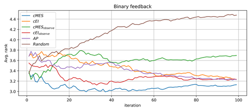
The results for the binary-feedback case in Table 2 and Figure 4 point to a number of conclusions. First, among methods operating in the unobserved scenario, cMES achieves the best overall average rank. While cEI uses fewer unfeasible evaluations, it is overly conservative and tends to converge to worse optima. Second, the AP baseline for is surprisingly effective, outperforming cEI. Third, using the value of in the unfeasible region, where the (unfeasible) global optimum resides, degrades performance for cMES. Finally, Figure 4 shows that cMES () is particularly efficient in early iterations, outperforming all competing methods by a wide margin. Individual results for each of the 10 optimization problems are given in Figure 8 of the supplemental material. We also compared all previous methods as well as PESC in the standard real-valued feedback, observed-objective scenario. The results over the 10 problems are summarized in Figure 5 and Table 3, showing that cMES outperforms competing approaches.
| Model | Dataset | Constraint | Threshold | Feasible points | |
|---|---|---|---|---|---|
| XGBoost | mg | model size | 50000 bytes | 72% | 7 (5, 2, 0) |
| Decision tree | mpg | model size | 3500 bytes | 48% | 4 (2, 1, 1) |
| Random forest | pyrim | model size | 5000 bytes | 26% | 4 (1, 2, 1) |
| Random forest | cpusmall | model size | 27000 bytes | 80% | 4(1, 2, 1) |
| MLP | pyrim | model size | 27000 bytes | 79% | 11 (5, 5, 1) |
| kNN + rnd. projection | australian | model size | 28000 bytes | 29% | 5 (1, 1, 3) |
| MLP | heart | error on neg. | 13.3% | 30% | 12 (6, 5, 1) |
| MLP | higgs | error on neg. | 60% | 38% | 12 (6, 5, 1) |
| Factorization machine | heart | error on neg. | 17% | 39% | 7 (3, 3, 1) |
| MLP | diabetes | error on neg. | 80% | 74% | 12 (6, 5, 1) |
| Optimizers | Unfeasible fraction | Ranking avg |
|---|---|---|
| 46.75 | 3.08 | |
| 33.01 | 3.43 | |
| 53.31 | 3.63 | |
| 40.44 | 3.26 | |
| 27.87 | 3.38 | |
| 49.83 | 4.21 |
| Optimizers | Unfeasible fraction | Ranking avg |
|---|---|---|
| 44.59 | 2.68 | |
| 40.84 | 3.0 | |
| 48.96 | 3.09 | |
| 27.87 | 2.79 | |
| 49.83 | 3.45 |



| Optimizers | Marginal | Joint |
|---|---|---|
| avg rank | avg rank | |
| 6.52 | 6.05 | |
| 6.1 | 5.77 | |
| 6.21 | 5.35 | |
| 7.24 | 7.04 | |
| 7.03 | 6.85 | |
| 7.36 | 6.45 |
| Optimizers | Avg rank |
|---|---|
| 5.55 | |
| 5.5 | |
| 5.22 | |
| 5.58 | |
| 5.48 | |
| 5.09 | |
| 5.59 | |
| 5.6 | |
| 5.49 | |
| 5.89 |
| Optimizers | Avg rank |
|---|---|
| 5.34 | |
| 5.73 | |
| 5.33 | |
| 5.87 | |
| 5.7 | |
| 5.4 | |
| 5.2 | |
| 5.68 | |
| 5.37 | |
| 5.4 |
All experiments with cMES draw the constrained optimum via joint sampling as described in Section 3. To gain more insight into the “mean field” assumption of [11], we reran cMES on the 10 constrained optimization problems using their marginal sampling approach to draw . The average rankings are reported in Table 4, where we draw 10 samples of at each iteration either via marginal or joint sampling, both in the observed and unobserved-objective settings and a range of values of . It is clear that marginal sampling degrades optimization performance across the board, confirming our observations from Section 3.
5 Conclusion
In this work, we introduced cMES, a novel acquisition function for Bayesian optimization in the presence of unknown constraints. Our proposed acquisition function can be used both with real-valued and binary constraint feedback. The binary case is relevant in practice, yet underserved in prior work. In an empirical comparison over a wide range of real-world HPO problems, cMES was shown to outperform baselines.
In future work, we will explore modalities where constraints can be evaluated independently of the objective. While cEI alone cannot be used to decide whether to evaluate or in isolation, as shown in our supplemental material it is easy to extend cMES to the separate evaluation case. Experiments with this mode as well as with multiple constraint functions are open directions for future work. We would also like to be able to more directly control the ratio of unfeasible evaluations, which requires changes to the policy beyond the acquisition function. Given our findings about shortcomings of the “mean field” independence assumption made in MES [11], it could also be important to find alternatives for posterior sampling of the constrained optimum . While joint posterior sampling works well in our experiments, its cubic scaling prevents usage for high-dimensional BO search spaces.
References
- [1] Jonas Mockus, Vytautas Tiesis, and Antanas Zilinskas. The application of Bayesian methods for seeking the extremum. Towards Global Optimization, 2(117-129):2, 1978.
- [2] Donald R Jones, Matthias Schonlau, and William J Welch. Efficient global optimization of expensive black-box functions. Journal of Global optimization, 13(4):455–492, 1998.
- [3] Bobak Shahriari, Kevin Swersky, Ziyu Wang, Ryan P Adams, and Nando de Freitas. Taking the human out of the loop: A review of Bayesian optimization. Proceedings of the IEEE, 104(1):148–175, 2016.
- [4] N. Srinivas, A. Krause, S. Kakade, and M. Seeger. Information-theoretic regret bounds for Gaussian process optimization in the bandit setting. IEEE Transactions on Information Theory, 58:3250–3265, 2012.
- [5] Jacob Gardner, Matt Kusner, Zhixiang Xu, Kilian Weinberger, and John Cunningham. Bayesian optimization with inequality constraints. In Proceedings of the International Conference on Machine Learning (ICML), pages 937–945, 2014.
- [6] Michael A. Gelbart, Jasper Snoek, and Ryan P. Adams. Bayesian optimization with unknown constraints. In Proceedings of the Thirtieth Conference on Uncertainty in Artificial Intelligence (UAI), pages 250–259, 2014.
- [7] José Miguel Hernández-Lobato, Michael A. Gelbart, Matthew W. Hoffman, Ryan P. Adams, and Zoubin Ghahramani. Predictive entropy search for Bayesian optimization with unknown constraints. In Proceedings of the International Conference on Machine Learning (ICML), pages 1699–1707, 2015.
- [8] P. Hennig and C. Schuler. Entropy search for information-efficient global optimization. Journal of Machine Learning Research, 13:1809–1837, 2012.
- [9] D. Hernandez-Lobato, J. Hernandez-Lobato, A. Shah, and R. Adams. Predictive entropy search for multi-objective Bayesian optimization. In M. Balcan and K. Weinberger, editors, International Conference on Machine Learning 33. JMLR.org, 2016.
- [10] José Miguel Hernández-Lobato, Michael A. Gelbart, Ryan P. Adams, Matthew W. Hoffman, and Zoubin Ghahramani. A general framework for constrained bayesian optimization using information-based search. Journal of Machine Learning Research, 17(160):1–53, 2016.
- [11] Z. Wang and S. Jegelka. Max-value entropy search for efficient Bayesian optimization. In D. Precup and Y. W. Teh, editors, International Conference on Machine Learning 34. JMLR.org, 2017.
- [12] K Eggensperger, F Hutter, HH Hoos, and K Leyton-brown. Efficient benchmarking of hyperparameter optimizers via surrogates background: Hyperparameter optimization. In Proceedings of the 29th AAAI Conference on Artificial Intelligence (AAAI), pages 1114–1120, 2012.
- [13] Carl Rasmussen and Chris Williams. Gaussian Processes for Machine Learning. MIT Press, 2006.
- [14] Jasper Snoek, Oren Rippel, Kevin Swersky, Ryan Kiros, Nadathur Satish, Narayanan Sundaram, Mostofa Patwary, Mr Prabhat, and Ryan Adams. Scalable Bayesian optimization using deep neural networks. In Proceedings of the International Conference on Machine Learning (ICML), pages 2171–2180, 2015.
- [15] Benjamin Letham, Brian Karrer, Guilherme Ottoni, and Eytan Bakshy. Constrained bayesian optimization with noisy experiments. Bayesian Analysis, 14(2):495–519, 2019.
- [16] V. Picheny, R. B. Gramacy, S. Wild, and S. Le Digabel. Bayesian optimization under mixed constraints with a slack-variable augmented Lagrangian. Advances in Neural Information Processing Systems 29, 2016.
- [17] Setareh Ariafar, Jaume Coll-Font, Dana Brooks, and Jennifer Dy. Admmbo: Bayesian optimization with unknown constraints using admm. Journal of Machine Learning Research, 20(123):1–26, 2019.
- [18] GPyOpt: A Bayesian optimization framework in Python. http://github.com/SheffieldML/GPyOpt, 2016.
- [19] T. Minka. Expectation propagation for approximate Bayesian inference. In J. Breese and D. Koller, editors, Uncertainty in Artificial Intelligence 17. Morgan Kaufmann, 2001.
- [20] C. Bishop. Pattern Recognition and Machine Learning. Springer, 1st edition, 2006.
- [21] W. Thompson. On the likelihood that one unknown probability exceeds another in view of theevidence of two samples. Biometrika, 25(3):285–294, 1933.
- [22] K. Kandasamy, A. Krishnamurthy, J. Schneider, and B. Poczos. Parallelised Bayesian optimisation via Thompson sampling. In A. Gretton and C. Robert, editors, Workshop on Artificial Intelligence and Statistics 19, pages 133–142, 2016.
- [23] Ilya M Sobol. On the distribution of points in a cube and the approximate evaluation of integrals. USSR Computational Mathematics and Mathematical Physics, 7(4):86–112, 1967.
- [24] James Bergstra and Yoshua Bengio. Random search for hyper-parameter optimization. Journal of Machine Learning Research (JMLR), 13:281–305, 2012.
- [25] Fabian Pedregosa, Gaël Varoquaux, Alexandre Gramfort, Vincent Michel, Bertrand Thirion, Olivier Grisel, Mathieu Blondel, Peter Prettenhofer, Ron Weiss, Vincent Dubourg, Jake Vanderplas, Alexandre Passos, David Cournapeau, Matthieu Brucher, Matthieu Perrot, and Édouard Duchesnay. Scikit-learn: Machine learning in Python. Journal of Machine Learning Research (JMLR), 12:2825–2830, 2011.
- [26] Chih-Chung Chang and Chih-Jen Lin. LIBSVM: A library for support vector machines. ACM Transactions on Intelligent Systems and Technology, 2:27:1–27:27, 2011.
- [27] M. Feurer, A. Klein, K. Eggensperger, J. Springenberg, M. Blum, and F. Hutter. Efficient and robust automated machine learning. In Advances in Neural Information Processing Systems 28, pages 2962–2970, 2015.
- [28] R. Bardenet, M. Brendel, B. Kégl, and M. Sebag. Collaborative hyperparameter tuning. In Proceedings of the International Conference on Machine Learning (ICML), pages 199–207, 2013.
- [29] A. Klein, Z. Dai, F. Hutter, N. Lawrence, and J. Gonzalez. Meta-surrogate benchmarking for hyperparameter optimization. arXiv:1905.12982, 2019.
Supplementary material
Appendix A Derivations
Consider the problem of Bayesian Optimization (BO) with unknown constraints. There are two real-valued functions , over a common space . The first models the criterion to be minimized, the second parameterizes the constraint. An evaluation produces , according to likelihood functions. First,
For , we consider two different options. In one scenario, we may observe directly, up to Gaussian noise:
In a different scenario, we may observe a binary target only:
Here, means the evaluation at is feasible, and means it is infeasible. We use the logistic parameterization, involving
but any other likelihood could be used instead. The constrained optimization problem we would like to solve is
| (2) |
Here, is a confidence parameter. In the case of binary feedback, , we can also write
where the confidence parameter is . Importantly, both and are unknown up front and have to be learned from noisy samples .
We assume that some data has already been acquired, based on which independent Gaussian posterior processes are obtained for and . The marginals of these are denoted by and , where we drop the indexing by . In the sequel, we drop both the conditioning on and on from the notation. For example, we write instead of :
The MES acquisition function [11] without constraints is given by:
where the expectation is over , and . Here, is a truncated Gaussian. It should be noted that this is a simplifying assumption. In PES [9], the related distribution is approximated, where is the argmin. Several local constraints on at are taken into account, such as . This is not done in MES, which simplifies derivations dramatically. Second, the expectation over is approximated by Monte Carlo sampling.
A.1 Real-valued Constraint Feedback
In this section, we assume that the constraint function can be observed directly, so that we obtain real-valued feedback from both and . Our generalization of MES to the constrained case uses
| (3) |
where the expectation is over , and is the constrained minimum (1). There are two points to be worked out:
- •
Expression for fixed
- •
Efficient approximate sampler from , where is given by (1), given that and are sampled from their respective posterior distributions (assumed to be independent).
In fact, the formulation so far ignores that we observe at , not , . Even though this is ignored in the original MES paper, a better acquisition function would therefore be
| (4) |
We start with the entropy difference in (3), where noise models are ignored, and come back to the noisy case (4) below. We will define in the same “local” way as in MES, avoiding all complications as considered in PES. What do we learn by conditioning on ? If , then . Otherwise (), our belief in remains the same. Therefore:
Here, we replaced by , which makes no difference for a distribution with a density. In the remainder of this section, is always over , unless otherwise indicated. Denote
We need some notation:
Here, , , is the cumulative distribution function for a standard normal variate. The normalization constant is
Also,
Note that the drops out, because . If we parameterize , , where are independent variates, we have that
Plugging this in:
At this point, we need the simple identity:
Concentrating on the final expectation term:
The hazard function of the standard normal is defined as
Noting that and , some algebra gives
Here, we used
All in all:
Note that , are negative. The only case when this expression becomes problematic is if both and tend to zero. This happens only if both is much smaller than and is much smaller than . If is sampled from , this is very unlikely to be the case. We need numerically robust code for computing and .
A.2 Entropy Difference for Noisy Targets
As noted above, we would ideally compute the entropy difference for the noisy targets instead of the latents , so use the acquisition function (4) instead of (3). How would this look like for the case where both and are real-valued with Gaussian likelihood? Define
where is defined as , but with being replaced by the posterior . Then:
To our knowledge, there is no simple closed-form expression for . The problem is that is not the product of a Gaussian with an indicator, and in particular is a complex function.
Here is a simple idea which may work better than just ignoring the noise and using (3). Complications arise because the expectations over and in do not result in a term which is the product of Gaussians and indicators. We can mitigate this problem by approximating with . Doing so results in
Here, , . Since is an affine function of , this can be brought into the same form as is used in the noise-free case, but is replaced by , by a different value, and by . Namely,
so that
We can now simply use the derivation from above. In fact,
just have to be used instead of .
A.3 Binary Constraint Feedback
For binary response , we have to take into account that much less information is obtained by sampling the constraint at . Here, a sensible approach is to ignore the noise on , but not ignore the likelihood . In other words, we can try to approximate
| (5) |
In this case, we use some approximate inference method for
where are Gaussians. In our current code, we use Laplace’s approximation, where mode finding is approximated by a single Newton step. Also, is using the highly accurate approximation given in [20, Sect. 4.5.2]. Now:
and
Importantly, is piece-wise constant, while not an indicator function anymore. Note that in general, due to the approximation we use, but it should be close.
In the following, is over , is over , and is over . First,
We split this in three parts, using the derivation of the noise-free case above. First:
Next:
Finally, note that if , then , so we can replace by , therefore:
Next, the expectation over . First,
so that
Next, using :
Finally,
Altogether, we obtain
We would compute , , , , then by logsumexp. In fact, if
then
The term is computed by folding the normalization into the argument inside , which is computed as
We then multiply with and sum over .
A.4 Sampling from
In the constrained case, we aim to sample from , where . Here, and are posterior GPs conditioned on the current data . At least for commonly used infinite-dimensional kernels, it is intractable to draw exact sample functions from these GPs, let alone to solve the conditional optimization problem for .
In [7], a finite-dimensional random kitchen sink (RKS) approximation is used to draw approximate sample paths, and the constrained problem is solved for these. Since the RKS basis functions are nonlinear in , so are objective and constraint function, and solving for requires complex machinery. A simpler approach is used in [11]. They target the cumulative distribution function (CDF) of , which can be written as expectation over and of an infinite product. This is approximated by restricting the product over a finite set , and by assuming independence of all and for . While this gives rise to a tractable approximation of the CDF, we found this approximation to be problematic in our experiments. As noted in [11], drawn under these assumptions are underbiased. In fact, due to the independence assumption, this bias gets worse the larger is: diverges as .
In our experiments, we follow [11] by restricting our attention to a finite set (we use a Sobol sequence [23]), but then draw joint samples of and respectively, based on which (restricted to ) is trivial to compute. While joint sampling scales cubically in the size of , sampling takes less than a second for , the size we used in our experiments.
More precisely, the posterior for conditioned on data is defined in terms of the Cholesky factor and the vector , where
where is the kernel matrix on the training set (), and is the noise precision. The posterior distribution of is a Gaussian with mean and covariance
where , , and . Samples of are drawn as
Due to the Cholesky factorization, joint sampling scales cubically in . On the other hand, sampling takes less than one second for sizes smaller than 2000.
A.5 Scoring Constraint or Criterion Evaluation
In some situations, we may be able to evaluate criterion and constraints independent of each other. For example, one may be much cheaper to evaluate than the other. To this end, we would like to score the value of sampling or at .
To this end, we just marginalize the joint distributions worked out above. First, consider the case where are real-valued, and we would like to score the value of sampling (the case of sampling is symmetric then). Note that this is the noisy case, where is replaced by , by , etc. We have that
Then, . Note that without the noise. In fact, the marginal does not depend on the noise , so the same expression is obtained in the case . In the following, we use that
Then:
Some algebra gives
By symmetry, if with Gaussian noise:
Finally, consider . Here,
Then:
Some algebra gives
where . Using the notation from above, this can also be written as
A.6 Observe only in Feasible Region
In this section, we deal with binary feedback . For some important applications, feedback on is obtained only if (feasible). For example, BO may be used to tune parameters of deep neural networks. A function evaluation of a test set metric may fail, because training crashed due to out of memory errors (). Note that itself does not depend on values of in the infeasible region.
It seems hard to properly define the entropy difference (conditioned on ) in this case. One idea is to simply use the entropy difference from Section A.3. Even though this assumes noise-free feedback for , the value conveys information about only if is feasible. Another idea is to consider the mixture of times the entropy difference from Section A.3 plus times the entropy difference from Section A.5. At least for away from , this could be a more reasonable score. Note that the part
appears in both entropy difference expressions.
Appendix B Real-world Hyperparameter Tuning Problems
We considered a range of 10 constrained HPO problems, spanning different scikitlearn algorithms [25], libsvm datasets [26], and constraint modalities. The first six problems are about optimizing an accuracy metric (AUC for binary classification, coefficient of determination for regression) subject to a constraint on model size, a setup motivated by applications in IOT or on mobile devices. The remaining four problems require minimizing the error on positives, subject to a limit on the error on negatives, as is relevant for example in applications in medical domains; here, one hyperparameter to tune is the fraction of the positive class in the data (both training and validation), which is adjusted by resampling with replacement. A summary of algorithms, datasets, and fraction of feasible configurations is given in Table 7. When sampling a problem, and then a hyperparameter configuration at random, we hit a feasible point with probability 51.5%. Also note that for all these problems, the overall global minimum point is unfeasible.
| Model | Dataset | Constraint | Threshold | Feasible points | |
|---|---|---|---|---|---|
| XGBoost | mg | model size | 50000 bytes | 72% | 7 (5, 2, 0) |
| Decision tree | mpg | model size | 3500 bytes | 48% | 4 (2, 1, 1) |
| Random forest | pyrim | model size | 5000 bytes | 26% | 4 (1, 2, 1) |
| Random forest | cpusmall | model size | 27000 bytes | 80% | 4(1, 2, 1) |
| MLP | pyrim | model size | 27000 bytes | 79% | 11 (5, 5, 1) |
| kNN + rnd. projection | australian | model size | 28000 bytes | 29% | 5 (1, 1, 3) |
| MLP | heart | error on neg. | 13.3% | 30% | 12 (6, 5, 1) |
| MLP | higgs | error on neg. | 60% | 38% | 12 (6, 5, 1) |
| Factorization machine | heart | error on neg. | 17% | 39% | 7 (3, 3, 1) |
| MLP | diabetes | error on neg. | 80% | 74% | 12 (6, 5, 1) |
All our example functions require a threshold, either on the size of trained model, or on the error on negatives. For a given HPO problem, the threshold is chosen as follows. First, we sample 2000 random values of the criterion function, without constraint. This allows us to access an effect of a particular threshold on the value of objective, and on a fraction of points which are unfeasible. We select a threshold at random, such that a total fraction of unfeasible points is between 20% and 80%. An example visualization for XGBoost is given in Figure 7.

The results for binary feedback on each individual blackbox are given in Figure 8, where we report the current minimum found up to each BO iteration for each competing method. Results are averaged over 20 repetitions and 95% confidence intervals on the minimal objective value are computed via boostrap.†† † www.github.com/facebookincubator/bootstrapped.


