跳到论文正文
W Papers独立论文阅读器 arXiv:1910.06871 论文正文 计算阅读时间 · 0%
引用这篇论文根据当前论文元数据生成,正式投稿前建议核对。


License: arXiv.org perpetual non-exclusive license
arXiv:1910.06871v4 [math.CO] 20 Nov 2020

Doctoral Dissertation

Combinatorial Analysis for Pseudoknot RNA with Complex Structure

By
Yangyang Zhao

A thesis submitted to the Graduate School of Nankai University

in partial fulfillment of the requirement for the degree of

Doctor of Philosophy

Nankai University

Tianjin, People’s Republic of China

March 2012

© Copyright 2012

Abstract

There exists many complicated kk-noncrossing pseudoknot RNA structures in nature based on some special conditions. The special characteristic of RNA structures gives us great challenges in researching the enumeration, prediction and the analysis of prediction algorithm. We will study two kinds of typical kk-noncrossing pseudoknot RNAs with complex structures separately.

The main content of Chapter 1 introduces the background and the significance of the project. We also present the chief results of this thesis.

In Chapter 2, we mainly illustrate the basic concepts, including the following items:

  1. 1.

    The construction of RNA, containing the secondary structures, pseudoknot structures and substructure of RNA.

  2. 2.

    Symbolic enumeration method. It is one of the most important method for studying the enumeration of RNA structures. All the generating functions are concluded by this method.

  3. 3.

    Combinatorial analysis, basic tool for asymptotically analyzing the enumeration of RNA structures. We mainly show DD-finiteness, PP-recursive, singularity analysis and distribution analysis in detail.

In Chapter 3, we discuss a kind of complicated structures named modular kk-noncrossing diagram. Such diagrams frequently appear in RNA prediction. The prediction program based on modular kk-noncrossing diagram is much more difficult to code. Therefore, we need to make the diagram clear, including the way of building it and the time complexity we build. To reach the purpose, we invent a whole new method to enumerate and find the asymptotic behavior of modular kk-noncrossing diagrams. The method is made with reconstructing VkV_{k}-shape, recurrence, differential equation and symbolic method. Finally we get the result that the asymptotic formula of the number of modular, kk-noncrossing diagram with nn nucleotides, which is,

𝖰k​(n)∼ck​n−((k−1)2+(k−1)/2)​(γk−1)n,k≥3,{\sf Q}_{k}(n)\sim c_{k}\,n^{-((k-1)^{2}+(k-1)/2)}\,(\gamma_{k}^{-1})^{n},\quad k\geq 3,

where γk\gamma_{k} is the minimum real solution of ϑ⁡(z)=ρk2\vartheta(z)=\rho_{k}^{2} and ckc_{k} is some positive constant, see eq. (3.4.28).

In Chapter 4, we emphasize the research on kk-noncrossing skeleton structure, especially when k=3k=3. The skeleton structure is well known in Huang’s folding algorithm for 33-noncrossing RNA structures. The algorithm constructs a skeleton tree first, in which every leaf is a skeleton structure. The structure of the skeleton tree is so complicated that the complexity of the algorithm is only concluded by experiment data in their paper. We will give a proof for the complexity and obtain the asymptotic formula of the number of canonical 33-noncrossing skeleton diagrams with nn vertices,

𝖲3[4]​(n)∼C′​n−5​(η−1)n,{\sf S}^{[4]}_{3}(n)\sim C^{\prime}\,n^{-5}\,(\eta^{-1})^{n},

where C′≈7892.16C^{\prime}\approx 7892.16, η≈0.4934\eta\approx 0.4934. Afterwards, we study the statistical properties of arcs in canonical 33-noncrossing skeleton diagrams. We prove the central limit theorem for arcs distributions in terms of their bivariate generating function. Our result allows to estimate the arc numbers in a random canonical 33-noncrossing skeleton diagrams.

Keywords: pseudoknot RNA, kk-noncrossing, matching, modular diagram, skeleton, symbolic enumeration, OGF, DD-finiteness, PP-recursive, singularity analysis, central limit law.

Chapter 1 Introduction

1.1 Background

The Ribonucleotide acid (RNA) is a single stranded molecule of four different nucleotides A, C, G and U, together with Watson-Crick (A-U, G-C) and (U-G) base pairs. It is one of the three major macromolecules that are essential for all known forms of life. The sequence of nucleotides allows RNA to encode genetic information. Over the decades of years, for the need of medicine and pharmacy, scientists give an intense interesting in the structure of RNA. The traditional way of researching RNA structure is cutting RNA by RNA enzyme or some reagent and analyzing by sequencing gel, which is time-consuming, high-tech demanding and expensive. To solve these problems, people turned to focus on using computer to predict a specific RNA structure.

Figure 1.1: HAR1F RF00635 RNA secondary structure represented as a planar graph. There are more than two isolated vertices in a hairpin marked by a dashed-line box.

RNA structures are separated into two categories, which are secondary structures and pseudoknot structures respectively. The secondary structures are the first been studied. In 1978, Waterman etc. completely investigate the combinatorial properties of secondary structure [44][45][29][37]. Assume that the number of secondary structures with nn nucleotides having arcs of length at least λ\lambda is 𝖳2[λ]​(n){\sf T}^{[\lambda]}_{2}(n). We have the recursion that

𝖳2[λ]​(n)=𝖳2[λ]​(n−1)+∑i=0n−λ−1𝖳2[λ]​(i)​𝖳2[λ]​(n−i−2),{\sf T}^{[\lambda]}_{2}(n)={\sf T}^{[\lambda]}_{2}(n-1)+\sum_{i=0}^{n-\lambda-1}{\sf T}^{[\lambda]}_{2}(i){\sf T}^{[\lambda]}_{2}(n-i-2), (1.1.1)

where 𝖳2[λ]​(n){\sf T}^{[\lambda]}_{2}(n) for 0≤n≤λ0\leq n\leq\lambda. The recursion above tells us the way of constructing an arbitrary secondary structure and it is also the fundamental of efficient minimum free energy folding (mfe) of RNA secondary structure [14, 13, 15]. The RNA secondary structure does not allow one or two isolated nucleotides in any one of hairpin loops, see Fig. 1.1** * The planar graph of HAR1F RF00635 is drawn by reference to http://en.wikipedia.org/wiki/File:HAR1F_RF00635_rna_secondary_structure.jpg..

Refer to caption
Figure 1.2: A planar graph of turnip yellow mosaic virus. The substructure marked by a dashed-line box is the pseudoknot.

There exists other RNA structures having cross-serial nucleotide interactions which is different from secondary structure. We call them pseudoknot structure [11]. The pseudoknot structure was first discovered in yellow mosaic virus in [41], see Fig. 1.2†† † The figure is cited from http://pseudoviewer.inha.ac.kr/Examples.htm.. Unlike the secondary structure, they are more complicated and hard to find a bijection between them and some combinatorial structure. It gives people who want to predict pseudoknot structures a big trouble. In 1999, Elena Rivas and Sean R. Eddy gave us a classical dynamic programming algorithm for RNA pseudoknot structure [36]. Meanwhile, Lynsø etc. [27] advanced a new predicting method based on a energy models. However, for the lack of the knowledge about the exact combinatorial meaning of pseudoknot, they cannot control the crossing number. For this reason, people began to study the combinatorial properties of RNA pseudoknot structure [17]. In the year of 2007, the paper [3] written by Chen and Stanley etc. showed us an involution combinatorial structure, “kk-noncrossing matching”. It actually builds a connection between a RNA pseudoknot structure and a kk-noncrossing matching. Based on this idea, Reidys etc. generalize the kk-noncrossing matching to specified kk-noncrossing diagram, which have bijection to the RNA pseudoknot structure [20][21][10]. Furthermore, the generating functions of some kinds of kk-noncrossing diagram were computed the asymptotic formula, which gives us a proof of growth rate when the number of nucleotides is increasing.

Figure 1.3: Modular kk-noncrossing diagrams: the inflation method. A modular 33-noncrossing diagram (top) is derived by inflating its 𝖵3{\sf V}_{3}-shape (bottom) in two steps. First we individually inflate each shape-arc into a more complex configuration and second insert isolated vertices (purple).

Around the year of 2010, Jin [19] focused on deriving the generating functions and asymptotic formula of 33-noncrossing diagram, while Han [10] focused on the diagram with 44 or higher cross number. Ma etc, [28] had further studies on some kk-noncrossing diagrams satisfying some constraints, i.e. kk-noncrossing τ\tau-canonical diagrams. The constraints specify minimum arc-length and stack-length of the diagrams, due to the biophysical constraints. All these kinds of diagrams belong to the class of diagrams, whose arc-length λ\lambda satisfies 1≤λ≤τ+11\leq\lambda\leq\tau+1. It means that the method used to compute the generating function and asymptotic formula of such a class of diagrams cannot be applied to some kk-noncrossing τ\tau-canonical diagram with arc length larger than τ+1\tau+1, such as kk-noncrossing 2-canonical diagrams with arc length not less than 4, which is also known as modular kk-noncrossing diagram. We have to develop a new way to treat this kind of diagrams. Fortunately, the 𝖵k{\sf V}_{k}-shapes will help us find the answer. It is like a core of a kk-noncrossing diagram. With an action called “inflation”, every kk-noncrossing diagrams can be produced by adding isolated vertices and stacks based on some 𝖵k{\sf V}_{k}-shape. The 𝖵k{\sf V}_{k}-shape in [32] can only be inflated to a kk-noncrossing τ\tau-canonical diagram with the arc length λ\lambda satisfying 1≤λ≤τ+11\leq\lambda\leq\tau+1. We have to reform the traditional 𝖵k{\sf V}_{k}-shape, called colored 𝖵k{\sf V}_{k}-shape, so as to adapt to the new problem. The main idea is to build modular kk-noncrossing diagrams via inflating their colored 𝖵k{\sf V}_{k}-shapes [33], see Fig. 1.3. The inflation gives rise to “stem-modules” over shape-arcs and is the key for the symbolic derivation of 𝐐k​(z){\bf Q}_{k}(z). One additional observation maybe worth to be pointed out: the computation of the generating function of colored shapes in Section 3.3, hinges on the intuition that the crossings of short arcs are relatively simple and give rise to manageable recursions. The coloring of these shapes then allows to identify the arc-configurations that require special attention during the inflation process. Our results are of importance in the context of RNA pseudoknot structures [35] and evolutionary optimization [31]. The method of generating modular kk-noncrossing diagrams gives contributions to analyze the joint structure [25][26].


Figure 1.4: An outline of cross[18]: the generation of motifs (I), the construction of skeleta-trees, that are rooted in irreducible shadows (II) and the saturation (III). During the latter we derive via DP-routines optimal fillings of intervals of skeleta. The red arrows represent the processing of two motifs, one of which leads to the generation of a skeleton tree, while the other leads directly to the saturation routine.

Besides modular kk-noncrossing diagram, another diagram, called skeleton diagram, is worth to study. It has a special characteristic that every arc is crossed by another arc. In the world of nature, the skeleton diagram rarely appears independently. However, skeleton diagram is an important substructure in every pseudoknot RNA structure. It is like a skeleton covering outside a pseudoknot diagram, and small substructures are filled in the “gap” of the skeleton diagrams, like muscle, see Fig. 1.5. Making the use of this special property, we can design a dynamic program to predict RNA structure. In 2008, Huang etc. [18] designed a folding 33-noncrossing algorithm, cross, based on the skeleton diagrams. The main idea is generating motifs first, then constructing a skeleta trees, rooted in irreducible shadows and saturation, during which via DP-routines, optimal fillings of skeleta-intervals are derived, see Fig. 1.4. The key difference to any other pseudoknot folding algorthm is the fact that cross has a transparent, combinatorially specified, output class. Cross is by design an algorithm of exponential time complexity by virtue of its construction of its skeleta-trees. Only in its saturation phase it employs vector versions of DP-routines. The fact shows us we must make clear the time complexity of generating skeleta-trees if we want to know the time complexity of the algorithm. It turns to be a problem that what the statistics property of the skeleta-trees is. Since any skeleton diagram can be found in a skeleta-tree, we need to find a way to enumerate the skeleton diagrams.

Figure 1.5: A skeleton diagram in a pseudoknot structure. The skeleton diagram is marked by thick line. The substructures marked by thin line are embedded in the intervals generated through splitting nucleotide (grey balls) sequence by the skeleton diagram.

1.2 Outline of the thesis

Besides introducing some basic concepts in this thesis, we mainly discuss about two subjects, which are the modular, kk-noncrossing diagrams and the 33-noncrossing skeleton diagrams, respectively. The thesis is organized as following.

In Chapter 1, we introduce the background and motivation of the thesis and illustrate the outline of the result and key method. The basic concepts and fundamental theorems which are highly used in the thesis, are present in Chapter 2.

The main results will be shown with the beginning of Chapter 3. The combinatorial analysis of modular, kk-noncrossing diagram is the main content of Chapter 3 . Based on 𝖵k{\sf V}_{k}-shape, we compute the generating function of colored shape, 𝐖k​(x,y,w){\bf W}_{k}(x,y,w) and 𝐈k​(x,y,z,w){\bf I}_{k}(x,y,z,w), which are

𝐖k​(x,y,w)=(1+x)​v​𝐅k​(x⁡(1+x)​v2),{\bf W}_{k}(x,y,w)=(1+x)v\,{\bf F}_{k}\left(x(1+x)v^{2}\right), (1.2.2)

and

𝐈k​(x,y,z,w,t)=1+xθ​𝐅k​(x⁡(1+(2​w−1)​x+(t−1)​x2)θ2),{\bf I}_{k}(x,y,z,w,t)=\frac{1+x}{\theta}{\bf F}_{k}\left(\frac{x(1+(2w-1)x+(t-1)x^{2})}{\theta^{2}}\right), (1.2.3)

where 𝐅k{\bf F}_{k} is the generating function of kk-noncrossing matching (see Section ) and

v\displaystyle v =\displaystyle= ((1−w)​x3+(1−w)​x2+(2−y)​x+1)−1\displaystyle\left((1-w)x^{3}+(1-w)x^{2}+(2-y)x+1\right)^{-1}
θ\displaystyle\theta =\displaystyle= 1−(y−2)​x+(2​w−z−1)​x2+(2​w−z−1)​x3\displaystyle 1-(y-2)x+(2w-z-1)x^{2}+(2w-z-1)x^{3}

for k>2k>2.

With help of the above two generating functions of colored shapes and symbolic enumeration method, we obtain the generating function of modular, kk-noncrossing diagrams when k>2k>2, which is

𝐐k​(z)\displaystyle{\bf Q}_{k}(z) =\displaystyle= 1−z2+z4q⁡(z)​𝐅k​(ϑ⁡(z)),\displaystyle\frac{1-z^{2}+z^{4}}{q(z)}{\bf F}_{k}\left(\vartheta(z)\right), (1.2.4)

where

q⁡(z)\displaystyle q(z) =\displaystyle= 1−z−z2+z3+2​z4+z6−z8+z10−z12\displaystyle 1-z-z^{2}+z^{3}+2z^{4}+z^{6}-z^{8}+z^{10}-z^{12}
ϑ⁡(z)\displaystyle\vartheta(z) =\displaystyle= z4​(1−z2−z4+2​z6−z8)q​(z)2.\displaystyle\frac{z^{4}(1-z^{2}-z^{4}+2z^{6}-z^{8})}{q(z)^{2}}. (1.2.5)

Eq. (1.2.4) shows us the generating function of modular, kk-noncrossing diagrams is composed of an rational expression and a composite function. Using the asymptotic method introduced in Chapter 2, we are able to conclude the asymptotic formula of modular, kk-noncrossing diagrams with nn vertices, which is

𝖰k​(n)∼ck​n−((k−1)2+(k−1)/2)​(γk−1)n,for some ck>0.{\sf Q}_{k}(n)\sim c_{k}\,n^{-((k-1)^{2}+(k-1)/2)}\,(\gamma_{k}^{-1})^{n},\quad\text{for some {$c_{k}>0$}}.

After we finish discussing about modular, kk-noncrossing diagram, we start to focus another interesting diagram, 33-noncrossing skeleton diagram, which will be studied in Chapter 4 [34]. Similarly as modular, kk-noncrossing diagram, the generating function of 33-noncrossing skeleton diagram should be given by inflating its shape (we call it 33-noncrossing skeleton shape), and the conclusion is

𝐒3[4]​(z)=(1−z)​𝐆​((w0​(z)​z1−z)2),{\bf S}^{[4]}_{3}(z)=(1-z){\bf G}\left(\left({{\sqrt{w_{0}(z)}z}\over{1-z}}\right)^{2}\right), (1.2.6)

where

𝐆⁡(x)=𝐒⁡(x)−1−x,w0​(z)=z41−z2+z6.\displaystyle{\bf G}(x)={\bf S}(x)-1-x,w_{0}(z)={z^{4}\over{1-z^{2}+z^{6}}}.

Here 𝐒⁡(x){\bf S}(x) is the generating function of 33-noncrossing skeleton shape. Before doing asymptotic of 33-noncrossing skeleton diagram, we must obtain the generating function of 𝐒⁡(x){\bf S}(x) and doing combinatorial analysis. The main idea is utilizing the relationship between skeleton diagram and irreducible structure [22] to compute the generating function of skeleton matching (a matching satisfying the condition of skeleton). Then we “shrink” the skeleton matching to the skeleton shape. Unlike the 33-noncrossing matching, the generating function of 33-noncrossing skeleton matching has no explicit formula. Thanks to the Bender’s theorem [2] and Eric’s method [8], we finally solve the asymptotic problem of 33-noncrossing skeleton matching, which is

𝖲⁡(h)∼C⋅h−5​R−h,{\sf S}(h)\ \sim\ C\cdot h^{-5}R^{-h},

where 𝖲⁡(h){\sf S}(h) is the number of 33-noncrossing skeleton matching with hh arcs and

C=24​(−512+165​π)53125​(256−81​π)5​π≈3.03096,R=256​(118−6415​π)2≈0.0729.\displaystyle C=\frac{24(-512+165\pi)^{5}}{3125(256-81\pi)^{5}\pi}\approx 3.03096,\quad R=256\left(\frac{11}{8}-\frac{64}{15\pi}\right)^{2}\approx 0.0729.

Using the asymptotic property of 33-noncrossing matching and eq. (1.2.6), we deduce that the asymptotic formula of 33-noncrossing skeleton diagram is

𝖲3[4]​(n)∼C′​n−5​(η−1)n,for some C′>0,{\sf S}^{[4]}_{3}(n)\sim C^{\prime}\,n^{-5}\,(\eta^{-1})^{n},\quad\text{for some {$C^{\prime}>0$}},

where 𝖲3[4]​(n){\sf S}^{[4]}_{3}(n) represents the number of canonical 33-noncrossing skeleton diagrams with nn vertices and C′≈7892.16C^{\prime}\approx 7892.16, η≈0.4934\eta\approx 0.4934.

Chapter 2 Basic concepts

In this chapter we provide the mathematical foundation of the thesis. The main object here is the generating function and asymptotic formula of kk-noncrossing matchings, which will play a central role for in RNA pseudoknot structures.

We begin with the nomenclatures and notations needed for the thesis. It contains two kinds of expressions for RNA pseudoknot structure, the elements in the RNA structure, diagram, and kk-noncrossing τ\tau-canonical, etc.

Next we introduce the fundamental combinatorial tools for obtaining the generating functions of kk-noncrossing diagrams. We use symbolic enumeration present by Flajolet [7] to get the generating function, avoiding the complicated recursive method.

After that we begin to discuss the combinatorial analyzing method for generating functions. The key method is the singularity analysis. However, before we introduce it, an important concept must be inducted, which is DD-finiteness. The DD-finiteness and singularity analysis are going to help us to analyze the generating function of kk-noncrossing diagrams asymptotically.

We then conclude this chapter by the central limit theorem due to Bender [1]. The central limit theorem shows that a sequence of random variables have a limit distribution Gaussian or normal distribution. The central limit theorem will be used in Chapter 4 to analyze the distribution of 33-noncrossing skeleton diagrams with nn vertices and hh arcs.

2.1 Nomenclatures and Notations

An arbitrary RNA structures can be uniquely expressed by two forms respectively, which are planar graph and diagram. A planar graph of RNA structure is a graph that obtained by embedding the 33-dimensional RNA structure into the plain, in which the nodes represent nucleotides and edges represent phosphodiester bond and Watson-Crick base pairs (A-U, G-C and U-G), see Fig. 1.2. If we “straighten” the edges representing phosphodiester bond, we will get the other expression, diagram. The strict definition of diagram follows

Definition 2.1.

A diagram is a labeled graph over the vertex set [n]=1,2,…,n[n]={1,2,\ldots,n}, represented by drawing its vertices on a horizonal line and its arcs (i,j)(i,j), i<ji<j in the upper half plain, where each vertex is connected with at most one arc, see Fig. 2.1. A vertex in a diagram is called an isolated vertex if there are not any arcs connecting with the vertex.

Figure 2.1: Features of a modular 33-noncrossing diagram represented as planar graph (top) and in diagram representation (bottom). We display a stack of length two (green), a stem of size two (red) and a 55-arc (blue).

Obviously, vertices and arcs correspond to nucleotides and Waston-Crick base pairs, respectively. In a diagram, a sequence of arcs (is,js)1≤s≤k{(i_{s},j_{s})}_{1\leq s\leq k} is called kk-nesting, if they satisfy

is<is−1<…<i2<i1<j1<j2<…<js−1<js.i_{s}<i_{s-1}<\ldots<i_{2}<i_{1}<j_{1}<j_{2}<\ldots<j_{s-1}<j_{s}.

Similarly, a sequence of arcs (is,js)1≤s≤k{(i_{s},j_{s})}_{1\leq s\leq k} is called kk-crossing if

i1<i2<…<ik<j1<j2<…<jk.i_{1}<i_{2}<\ldots<i_{k}<j_{1}<j_{2}<\ldots<j_{k}.

Similarly, If a diagram have k−1k-1-crossing arcs at most, we call it kk-noncrossing diagram. Particularly, if kk equals 2, the diagram will degenerate to noncrossing diagram, which corresponds to secondary structure.

A kk-noncrossing, τ\tau-canonical structure, is a diagram in which

  • •

    there exists no kk-crossing arcs,

  • •

    stack has at least size τ\tau, and

  • •

    any arc (i,j)(i,j) has a minimum arc length j−i≥2j-i\geq 2

We next specify further properties of kk-noncrossing diagrams:

  • •

    a stack of size σ\sigma, Si,jσS_{i,j}^{\sigma}, is a maximal sequence of “parallel” arcs,

    ((i,j),(i+1,j−1),…,(i+(σ−1),j−(σ−1))).((i,j),(i+1,j-1),\dots,(i+(\sigma-1),j-(\sigma-1))).

    We call a stack of size σ\sigma a σ\sigma-stack,

  • •

    a stem of size ss is a sequence

    (Si1,j1σ1,Si2,j2σ2,…,Sis,jsσs)\left(S_{i_{1},j_{1}}^{\sigma_{1}},S_{i_{2},j_{2}}^{\sigma_{2}},\ldots,S_{i_{s},j_{s}}^{\sigma_{s}}\right)

    where Sim,jmσmS_{i_{m},j_{m}}^{\sigma_{m}} is nested in Sim−1,jm−1σm−1S_{i_{m-1},j_{m-1}}^{\sigma_{m-1}} such that any arc nested in Sim−1,jm−1σm−1S_{i_{m-1},j_{m-1}}^{\sigma_{m-1}} is either contained or nested in Sim,jmσmS_{i_{m},j_{m}}^{\sigma_{m}}, for 2≤m≤s2\leq m\leq s.

For an illustration of the above structural features, see Fig. 2.1. Note that given a stem

(Si1,j1σ1,Si2,j2σ2,…,Sis,jsσs)\left(S_{i_{1},j_{1}}^{\sigma_{1}},S_{i_{2},j_{2}}^{\sigma_{2}},\ldots,S_{i_{s},j_{s}}^{\sigma_{s}}\right)

the maximality of the stacks implies that any two nested stacks within a stem, Sim,jmσmS_{i_{m},j_{m}}^{\sigma_{m}} and Sim−1,jm−1σm−1S_{i_{m-1},j_{m-1}}^{\sigma_{m-1}} are separated by a nonempty interval of isolated vertices between im−1+(σm−1−1)i_{m-1}+(\sigma_{m-1}-1) and imi_{m} or jm−1−(σm−1−1)j_{m-1}-(\sigma_{m-1}-1) and jmj_{m}, respectively.

2.2 Symbolic enumeration method

When we deal with the enumeration of diagrams, we actually deal with d​i​s​c​r​e​t​ediscrete objects, which can be finitely described by constructions rules. For example, the vertices, arcs, stacks and stems in kk-noncrossing RNA structures. Our major is to enumerate such objects according to some characteristics parameter(s).

Definition 2.2.

A combinatorial class, or simply a class, is a finite or denumerable set on which a size function is defined, satisfying the following conditions: (i) the size of an element is a non-negative integer; (ii) the number of elements of any given size is finite.

Definition 2.3.

The counting sequence of a combinatorial class is the sequence of integers (an)n≥0(a_{n})_{n\geq 0} where an=card⁡(an)a_{n}={\rm card}(a_{n}) is the number of objects in class 𝒜\mathcal{A} that have size nn.

Next, for combinatorial enumeration purposes, it is convenient to identify combinatorial classes that are merely variants of one another.

Definition 2.4.

Two combinatorial classes 𝒜\mathcal{A} and ℬ\mathcal{B} are said to be (combinatorially) isomorphic, which is written 𝒜≅ℬ\mathcal{A}\cong\mathcal{B}, iff their counting sequences are identical. This condition is equivalent to the existence of a bijection from 𝒜\mathcal{A} to ℬ\mathcal{B} that preserves size, and one also says that 𝒜\mathcal{A} and ℬ\mathcal{B} are bijectively equivalent.

Suppose we have a combinatorial class and the corresponding counting sequence. We define the ordinary generating function (OGF) as follows.

Definition 2.5.

The ordinary generating function (OGF) of a sequence (an)(a_{n}) is the formal power series

A⁡(z)=∑n=0∞an​zn.A(z)=\sum_{n=0}^{\infty}a_{n}z^{n}. (2.2.1)

The ordiary generating function (OGF) of a combinatorial class 𝒜\mathcal{A} is the generating function of the number An=card⁡(an)A_{n}={\rm card}(a_{n}). Equivalently, the OGF of class 𝒜\mathcal{A} admits the combinatorial form

A⁡(z)=∑α∈𝒜z|α|.A(z)=\sum_{\alpha\in\mathcal{A}}z^{|\alpha|}. (2.2.2)

It is also said that the variable zz marks size in the generating function

The combinatorial form of an OGF in eq. (2.2.2) results straightforwardly from observing that the term znz^{n} occurs as many times as there are objects in 𝔸\mathbb{A} having size nn.

We let generally [zn]​f​(z)[z^{n}]f(z) denote the operation of extracting the coefficient of znz^{n} in the formal power series f⁡(z)=∑fn​znf(z)=\sum f_{n}z^{n}, so that

[zn]​(∑n≥0fn​zn)=fn[z^{n}]\left(\sum_{n\geq 0}f_{n}z^{n}\right)=f_{n} (2.2.3)
Example 2.1.

Noncrossing matching. Let ℳ\mathcal{M} be the class of the noncrossing matchings. Then ℳ\mathcal{M} can be represented as

ℳ:={ε,{(1,2)},{(1,2),(3,4)},{(1,4),(2,3)},…},\mathcal{M}:=\{\varepsilon,\{(1,2)\},\{(1,2),(3,4)\},\{(1,4),(2,3)\},\ldots\},

where ε\varepsilon is an empty noncrossing matching without arcs. For the matching γ={(1,2),(3,4)}\gamma=\{(1,2),(3,4)\} we have |γ|=2|\gamma|=2. We already know the number of noncrossing matching with nn arcs is cn=1n+1​(2​nn)c_{n}=\frac{1}{n+1}{{2n}\choose n}. Therefore we have the following equations,

M⁡(z)=∑γ∈ℳzγ=∑n≥0cn​zn=1−1−4​z2​z.M(z)=\sum_{\gamma\in\mathcal{M}}z^{\gamma}=\sum_{n\geq 0}c_{n}z^{n}=\frac{1-\sqrt{1-4z}}{2z}.

Now we start to learn about the basic constructions that constitute the core of a specification language for combinatorial structures. For the demand of the thesis, we mainly discuss about disjoint union, Cartesian product and sequence construction.

First, assume we are given a class ℰ\mathcal{E} called the neutral class that consists of a single object of size 00, and a class 𝒵\mathcal{Z} called an atomic class comprising a single element of size 11. Clearly, the generating functions of a neutral class ℰ\mathcal{E} and an atomic class 𝒵\mathcal{Z} are

E⁡(z)=1,Z⁡(z)=z,E(z)=1,\qquad Z(z)=z,

corresponding to the unit 1,and the variable zz, of generating functions.

Proposition 2.1.

Let 𝒜\mathcal{A}, ℬ\mathcal{B}, 𝒞\mathcal{C} be combinatorial classes. AnA_{n}, BnB_{n}, CnC_{n} are the corresponding cardinals of size nn and A⁡(x)A(x), B⁡(x)B(x), C⁡(x)C(x) are the corresponding ordinary generating functions.

  1. 1.

    Disjoint union. 𝒜\mathcal{A}, ℬ\mathcal{B} and 𝒞\mathcal{C} satisfy

    𝒜=ℬ∪𝒞,withℬ∩𝒞=∅,\mathcal{A}=\mathcal{B}\cup\mathcal{C},\qquad\text{with}\quad\mathcal{B}\cap\mathcal{C}=\emptyset, (2.2.4)

    with size defined in a consistent manner: for ω∈𝒜\omega\in\mathcal{A},

    |ω|𝒜={|ω|ℬif ω∈ℬ|ω|𝒞if ω∈𝒞.|\omega|_{\mathcal{A}}=\begin{cases}|\omega|_{\mathcal{B}}&\quad\text{if $\omega\in\mathcal{B}$}\\ |\omega|_{\mathcal{C}}&\quad\text{if $\omega\in\mathcal{C}$}.\end{cases} (2.2.5)

    One has

    An=Bn+Cn,A_{n}=B_{n}+C_{n}, (2.2.6)

    which, at generating function level, means

    A⁡(z)=B⁡(z)+C⁡(z).A(z)=B(z)+C(z). (2.2.7)
  2. 2.

    Cartesian product. This construction applied to two classes ℬ\mathcal{B} and 𝒞\mathcal{C} forms ordered pairs,

    𝒜=ℬ×𝒞iff𝒜={α=(β,γ)∣β∈ℬ,γ∈𝒞},\mathcal{A}=\mathcal{B}\times\mathcal{C}\quad\text{iff}\quad\mathcal{A}=\{\alpha=(\beta,\gamma)\mid\beta\in\mathcal{B},\gamma\in\mathcal{C}\}, (2.2.8)

    with the size of a pair α=(β,γ)\alpha=(\beta,\gamma) being defined by

    |α|𝒜=|β|ℬ+|​γ|𝒞.|\alpha|_{\mathcal{A}}=|\beta|_{\mathcal{B}}+|\gamma|_{\mathcal{C}}. (2.2.9)

    It is immediately seen that the counting sequences corresponding to 𝒜,ℬ,𝒞\mathcal{A},\mathcal{B},\mathcal{C} are related by the convolution relation

    An=∑k=0nBk​Cn−k,A_{n}=\sum_{k=0}^{n}B_{k}C_{n-k}, (2.2.10)

    which means admissibility. Furthermore, we recognize here the formula for a product of two power series,

    A⁡(z)=B⁡(z)⋅C⁡(z).A(z)=B(z)\cdot C(z). (2.2.11)
  3. 3.

    Sequence construction. If ℬ\mathcal{B} is a class then the sequence class Seq(ℬ)(\mathcal{B}) is defined as the infinite sum

    Seq​(ℬ)={ϵ}+ℬ+ℬ×ℬ+⋯\textsc{Seq}(\mathcal{B})=\{\epsilon\}+\mathcal{B}+\mathcal{B}\times\mathcal{B}+\cdots (2.2.12)

    with ϵ\epsilon being a neutral structure. In other words, we have

    𝒜={(β1,…,βℓ)∣ℓ≥0,βj∈ℬ}.\mathcal{A}=\left\{(\beta_{1},\ldots,\beta_{\ell})\mid\ell\geq 0,\beta_{j}\in\mathcal{B}\right\}.

    According cartesian product and eq. (2.2.12), the generating function of 𝒜\mathcal{A} will hold as follows,

    A⁡(z)=1+B⁡(z)+B⁡(z)⋅B⁡(z)+⋯=11−B⁡(z).A(z)=1+B(z)+B(z)\cdot B(z)+\cdots=\frac{1}{1-B(z)}. (2.2.13)
Example 2.2.

Interval coverings. Let 𝒵:=a\mathcal{Z}:={a}. Then 𝒜=𝒵+𝒵×𝒵\mathcal{A}=\mathcal{Z}+\mathcal{Z}\times\mathcal{Z} is a set of two elements, aa and (a,a)(a,a), which we choose to note as {a,a​a}\{a,aa\}. Then 𝒞=Seq​(𝒜)\mathcal{C}=\textsc{Seq}(\mathcal{A}) contains

a,a​a,a​a,a​a​a,a​a​a,a​a​a​a,a​a​a​a,…a,a\ a,aa,a\ aa,aa\ a,aa\ aa,a\ a\ a\ a,\ldots

with the notion of size adopted, the objects of size nn in 𝒞=Seq​(𝒵+𝒵×𝒵)\mathcal{C}=\textsc{Seq}(\mathcal{Z}+\mathcal{Z}\times\mathcal{Z}) are isomorphic to the covering of [0,n][0,n] by intervals of length either 1 or 2. The OGF

C⁡(z)=1+z+2​z2+3​z3+5​z4+⋯=11−z−z2.C(z)=1+z+2z^{2}+3z^{3}+5z^{4}+\cdots=\frac{1}{1-z-z^{2}}.

2.3 DD-finiteness and PP-recursive

DD-finiteness and PP-recursive are important concepts in the asymptotics of kk-noncrossing diagrams. In Chapter 3, we will use these two concepts to do the asymptotic of modular kk-noncrossing diagrams. Based on the paper of Stanley [38], an arbitrary power series, S⁡(x)=∑n≥0sn​xnS(x)=\sum_{n\geq 0}s_{n}x^{n} is analytically continuated in any simply-connected domain containing zero avoiding singularities if S⁡(x)S(x) is DD-finite.

Definition 2.6 ([39]).

(a) A sequence f⁡(n)f(n) of complex number is said to be PP-recursive, if there are polynomials p0​(n),…,pm​(n)∈ℂ⁡[n]p_{0}(n),\ldots,p_{m}(n)\in\mathbb{C}[n] with pm​(n)≠0p_{m}(n)\neq 0, such that for all n∈ℕn\in\mathbb{N}

pm​(n)​f​(n+m)+pm−1​(n)​f​(n+m−1)+⋯+p0​(n)​f​(n)=0.p_{m}(n)f(n+m)+p_{m-1}(n)f(n+m-1)+\cdots+p_{0}(n)f(n)=0. (2.3.14)

(b) A formal power series F⁡(x)=∑n≥0f⁡(n)​xnF(x)=\sum_{n\geq 0}f(n)x^{n} is rational, if there are polynomials A⁡(x)A(x) and B⁡(x)B(x) in ℂ⁡[x]\mathbb{C}[x] with B⁡(x)≠0B(x)\neq 0, such that

F⁡(x)=A⁡(x)B⁡(x).F(x)=\frac{A(x)}{B(x)}.

(c) F⁡(x)F(x) is algebraic of degree mm, if there exist polynomials q0​(x),…,qm​(x)∈ℂ⁡[x]q_{0}(x),\ldots,q_{m}(x)\in\mathbb{C}[x] with qm​(x)≠0q_{m}(x)\neq 0, such that

qm​(x)​Fm​(x)+qm−1​(x)​Fm−1​(x)+⋯+q1​(x)​F​(x)+q0​(x)=0.q_{m}(x)F^{m}(x)+q_{m-1}(x)F^{m-1}(x)+\cdots+q_{1}(x)F(x)+q_{0}(x)=0.

(d) F⁡(x)F(x) is DD-finite, if there are polynomials q0​(x),…,qm​(x)∈ℂ⁡[x]q_{0}(x),\ldots,q_{m}(x)\in\mathbb{C}[x] with qm​(x)≠0q_{m}(x)\neq 0, such that

qm​(x)​F(m)​(x)+qm−1​(x)​F(m−1)​(x)+⋯+q1​(x)​F′​(x)+q0​(x)​F​(x)=0,q_{m}(x)F^{(m)}(x)+q_{m-1}(x)F^{(m-1)}(x)+\cdots+q_{1}(x)F^{\prime}(x)+q_{0}(x)F(x)=0, (2.3.15)

where F(i)​(x)=di​F​(x)/d​xiF^{(i)}(x)=d^{i}F(x)/dx^{i}, and ℂ⁡[x]\mathbb{C}[x] is the ring of polynomials in xx with complex coefficients.

Let ℂ⁡(x)\mathbb{C}(x) denote the rational function field, i.e. the field generated by taking equivalence classes of fractions of polynomials. Let ℂalg​[[x]]\mathbb{C}_{\text{\rm alg}}[[x]] and 𝒟\mathcal{D} denote the sets of algebraic power series over ℂ⁡(x)\mathbb{C}(x) and DD-finite power series, respectively. The four definitions above actually can imply the following theorem.

Theorem 2.2 ([39]).
  1. 1.

    A rational power series is algebraic.

  2. 2.

    Let F∈ℂ⁡[[x]]F\in\mathbb{C}[[x]] be algebraic of degree mm. Then FF is DD-finite.

  3. 3.

    Let F=∑n≥0f⁡(n)​xn∈ℂ⁡[[x]]F=\sum_{n\geq 0}{f(n)x^{n}}\in\mathbb{C}[[x]], then FF is DD-finite if and only if ff is PP-recursive.

Proof.
  1. 1.

    Here we use the notations of Definition 2.6 (b). Let q0​(x)=−A​(x)q_{0}(x)=-A(x), q1​(x)=B​(x)q_{1}(x)=B(x), then we have B⁡(x)​F​(x)−A⁡(x)=0B(x)F(x)-A(x)=0. Therefore FF is algebraic.

  2. 2.

    Using the notations of Definition 2.6 (c), let P⁡(x,y)∈ℂ⁡[x,y]P(x,y)\in\mathbb{C}[x,y] and nonzero,

    P⁡(x,F)=qm​(x)​Fm​(x)+qm−1​(x)​Fm−1​(x)+⋯+q1​(x)​F​(x)+q0​(x),P(x,F)=q_{m}(x)F^{m}(x)+q_{m-1}(x)F^{m-1}(x)+\cdots+q_{1}(x)F(x)+q_{0}(x), (2.3.16)

    then we have

    0=dd​x​P​(x,F)=∂P⁡(x,y)∂x|y=F+F′​∂P⁡(x,y)∂y|y=F.0=\frac{\text{d}}{\text{d}x}P(x,F)=\frac{\partial P(x,y)}{\partial x}\big|_{y=F}+F^{\prime}\frac{\partial P(x,y)}{\partial y}\big|_{y=F}. (2.3.17)

    It therefore follows that

    F′=−∂P⁡(x,y)∂x|y=F∂P⁡(x,y)∂y|y=F∈ℂ⁡(x,F).F^{\prime}=-\frac{\frac{\partial P(x,y)}{\partial x}\big|_{y=F}}{\frac{\partial P(x,y)}{\partial y}\big|_{y=F}}\in\mathbb{C}(x,F). (2.3.18)

    Continually differentiating eq. (2.3.18) with respect to xx shows by induction that F(k)∈ℂ⁡(x,F)F^{(k)}\in\mathbb{C}(x,F) for all k≥0k\geq 0. But dimℂ⁡(x)​ℂ​(x,F)=m\text{dim}_{\mathbb{C}(x)}\mathbb{C}(x,F)=m, so F,F′,…,F(m)F,F^{\prime},\ldots,F^{(m)} are linearly dependent over ℂ⁡(x)\mathbb{C}(x), yielding an equation of the form eq. (2.3.15). The DD-finiteness of FF is proved.

  3. 3.

    Suppose FF is DD-finite, so that eq. (2.3.15) holds (with qm≠0q_{m}\neq 0). Since

    xj​F(i)=∑n≥0(n+i−j)i​f​(n+i−j)​xn,x^{j}F^{(i)}=\sum_{n\geq 0}(n+i-j)_{i}f(n+i-j)x^{n}, (2.3.19)

    when we equate coefficients of xn+kx^{n+k} in eq. (2.3.15) for fixed kk sufficiently large, we will obtain a recurrence of the form eq. (2.3.14). This recurrence will not collapse to 0=00=0 because if [xj]​qm​(x)≠0[x^{j}]q_{m}(x)\neq 0, then [nd]​pm−j+k​(n)≠0[n^{d}]p_{m-j+k}(n)\neq 0. Conversely, suppose that ff satisfies eq. (2.3.14) with pm​(n)≠0p_{m}(n)\neq 0. For fixed i∈ℕi\in\mathbb{N}, the polynomials (n+i)j(n+i)_{j}, j≥0j\geq 0, form a ℂ\mathbb{C}-basis for the space ℂ⁡[n]\mathbb{C}[n] (since OPENdeg⁡(n+i)j)=j\deg(n+i)_{j})=j). Thus pi​(n)p_{i}(n) is a ℂ\mathbb{C}-linear combination of the polynomials (n+i)j(n+i)_{j}, so ∑n≥0pi​f​(n+i)​xn\sum_{n\geq 0}p_{i}f(n+i)x^{n} is a ℂ\mathbb{C}-linear combination of series of the form ∑n≥0(n+i)j​f​(n+i)​xn\sum_{n\geq 0}(n+i)_{j}f(n+i)x^{n}. Now

    ∑n≥0(n+i)j​f​(n+i)​xn=Ri​(x)+xj−i​F(j)\sum_{n\geq 0}(n+i)_{j}f(n+i)x^{n}=R_{i}(x)+x^{j-i}F^{(j)} (2.3.20)

    for some Ri​(x)∈x−1​ℂ​[x−1]R_{i}(x)\in x^{-1}\mathbb{C}[x^{-1}] (i.e. Ri​(x)R_{i}(x) is a Laurent polynomial all of whose exponents are negative). Hence multiplying eq. (2.3.14) by xnx^{n} and summing on n≥0n\geq 0 yields

    0=∑ai​j​xj−i​F(j)+R⁡(x),0=\sum a_{ij}x^{j-i}F^{(j)}+R(x), (2.3.21)

    where the sum is finite, ai​j∈ℂa_{ij}\in\mathbb{C} and R⁡(x)∈x−1​ℂ​[x−1]R(x)\in x^{-1}\mathbb{C}[x^{-1}]. One easily sees that not all ai​j=0a_{ij}=0. Now multiply eq. (2.3.21) by xqx^{q} for qq sufficiently large to get an equation of the form eq. (2.3.15).


For easily understanding, we present an example.

Example 2.3.

The Motzkin number MnM_{n} are defined by

M⁡(x)\displaystyle M(x) =∑n≥0Mn​xn=1−x−1−2​x−3​x22​x2\displaystyle=\sum_{n\geq 0}M_{n}x^{n}=\frac{1-x-\sqrt{1-2x-3x^{2}}}{2x^{2}}
=1+x+2​x2+4​x3+9​x4+21​x5+51​x6+⋯,\displaystyle=1+x+2x^{2}+4x^{3}+9x^{4}+21x^{5}+51x^{6}+\cdots,

M⁡(x)M(x) is algebraic and DD-finite since

x2​M​(x)2+(x−1)​M​(x)+1=0x^{2}M(x)^{2}+(x-1)M(x)+1=0

and

(6​x+3)​M​(x)+(12​x2+7​x−3)​M′​(x)+x⁡(x+1)​(3​x−1)​M′′​(x)=0(6x+3)M(x)+(12x^{2}+7x-3)M^{\prime}(x)+x(x+1)(3x-1)M^{\prime\prime}(x)=0

which implies MnM_{n} is PP-recursive since

−(n2+4​n+3)​Mn+1+(2​n2+5​n+3)​Mn+(3​n2+3​n)​Mn−1=0-(n^{2}+4n+3)M_{n+1}+(2n^{2}+5n+3)M_{n}+(3n^{2}+3n)M_{n-1}=0

We proceed by studying closure properties of DD-finite power series which are of key important in the following chapters.

Theorem 2.3.

[39] PP-recursive sequences, DD-finite and algebraic power series have the following properties:
(a) If f,gf,g are PP-recursive, then f⋅gf\cdot g is PP-recursive.
(b) If F,G∈𝒟F,G\in\mathcal{D}, and α,β∈ℂ\alpha,\beta\in\mathbb{C}, then α​F+β​G∈𝒟\alpha F+\beta G\in\mathcal{D} and F​G∈𝒟FG\in\mathcal{D}.
(c) If F∈𝒟F\in\mathcal{D} and G∈ℂa​l​g​[[x]]G\in\mathbb{C}_{alg}[[x]] with G⁡(0)=0G(0)=0, then F⁡(G⁡(x))∈𝒟F(G(x))\in\mathcal{D}.

Here we omit the proof of (a) and (b) which can be found in [39]. We present however a direct proof of (c).

Proof.

(c) We assume that G⁡(0)=0G(0)=0 so that the composition F⁡(G⁡(x))F(G(x)) is well-defined. Let K=F⁡(G⁡(x))K=F(G(x)). Then K(i)K^{(i)} is a linear combination of F⁡(G⁡(x)),F′​(G⁡(x)),…F(G(x)),\,F^{\prime}(G(x)),\,\ldots over ℂ⁡[G,G′,…]\mathbb{C}[G,\,G^{\prime},\ldots], i.e. the ring of polynomials in G,G′,…G,\,G^{\prime},\ldots with complex coefficients.
Claim. G(i)∈ℂ⁡(x,G),i≥0G^{(i)}\in\mathbb{C}(x,G),\ i\geq 0 and therefore ℂ⁡[G,G′,…]⊂ℂ⁡(x,G)\mathbb{C}[G,\,G^{\prime},\ldots]\subset\mathbb{C}(x,G), where ℂ⁡(x,G)\mathbb{C}(x,G) denotes the field generated by xx and GG.
Since GG is algebraic, it satisfies

qd​(x)​Gd​(x)+qd−1​(x)​Gd−1​(x)+⋯+q1​(x)​G​(x)+q0​(x)=0,q_{d}(x)G^{d}(x)+q_{d-1}(x)G^{d-1}(x)+\cdots+q_{1}(x)G(x)+q_{0}(x)=0, (2.3.22)

where q0​(x),…,qd​(x)∈ℂ⁡[x],qd​(x)≠0q_{0}(x),\ldots,q_{d}(x)\in\mathbb{C}[x],\ q_{d}(x)\neq 0 and dd is minimal, i.e. (Gi​(x))i=0d−1(G^{i}(x))_{i=0}^{d-1} is linear independent over ℂ⁡[x]\mathbb{C}[x]. In other words, for all (q~i​(x))i=1d−1≠0(\widetilde{q}_{i}(x))_{i=1}^{d-1}\neq 0 we have

q~d−1​(x)​Gd−1​(x)+⋯+q~1​(x)​G​(x)+q~0​(x)≠0.\widetilde{q}_{d-1}(x)G^{d-1}(x)+\cdots+\widetilde{q}_{1}(x)G(x)+\widetilde{q}_{0}(x)\neq 0.

We consider

P⁡(x,G)=qd​(x)​Gd​(x)+qd−1​(x)​Gd−1​(x)+⋯+q1​(x)​G​(x)+q0​(x).P(x,G)=q_{d}(x)G^{d}(x)+q_{d-1}(x)G^{d-1}(x)+\cdots+q_{1}(x)G(x)+q_{0}(x).

Differentiating eq. (2.3.22) once, we derive

0=dd​x​P​(x,G)=∂P⁡(x,y)∂x|y=G+G′​∂P⁡(x,y)∂y|y=G.0=\frac{d}{dx}P(x,G)=\frac{\partial P(x,y)}{\partial x}\Big|_{y=G}+G^{\prime}\frac{\partial P(x,y)}{\partial y}\Big|_{y=G}.

The degree of ∂P⁡(x,y)∂y|y=G\frac{\partial P(x,y)}{\partial y}\Big|_{y=G} in GG is d−1d-1 and qd​(x)≠0q_{d}(x)\neq 0, whence ∂P⁡(x,y)∂y|y=G≠0\frac{\partial P(x,y)}{\partial y}\Big|_{y=G}\neq 0. We therefore arrive at

G′=−∂P⁡(x,y)∂x|y=G∂P⁡(x,y)∂y|y=G∈ℂ⁡(x,G).G^{\prime}=-~\frac{\frac{\partial P(x,y)}{\partial x}\Big|_{y=G}}{\frac{\partial P(x,y)}{\partial y}\Big|_{y=G}}\,\in\mathbb{C}(x,G).

Iterating the above argument, we obtain G(i)∈ℂ⁡(x,G),i≥0G^{(i)}\in\mathbb{C}(x,G),\ i\geq 0 and therefore ℂ⁡[G,G′,…]⊂ℂ⁡(x,G)\mathbb{C}[G,\,G^{\prime},\ldots]\subset\mathbb{C}(x,G), whence the Claim.
Let V~\widetilde{V} be the ℂ⁡(x,G)\mathbb{C}(x,G) vector space spanned by F⁡(G⁡(x)),F′​(G⁡(x)),…F(G(x)),\,F^{\prime}(G(x)),\,\ldots. Since F∈𝒟F\in\mathcal{D}, we have dimℂ⁡(x)​⟨F,F′,⋯⟩<∞\text{dim}_{\mathbb{C}(x)}\langle F,F^{\prime},\cdots\rangle<\infty, immediately implying the finiteness of dimℂ⁡(G)​⟨F⁡(G),F′​(G),⋯⟩\text{dim}_{\mathbb{C}(G)}\langle F(G),F^{\prime}(G),\cdots\rangle. Thus, since ℂ⁡(G)\mathbb{C}(G) is a subfield of ℂ⁡(x,G)\mathbb{C}(x,G), we derive

dimℂ⁡(x,G)​⟨F,F′,⋯⟩<∞\text{dim}_{\mathbb{C}(x,G)}\langle F,F^{\prime},\cdots\rangle<\infty

and consequently dimℂ⁡(x,G)​V~<∞\text{dim}_{\mathbb{C}(x,G)}\widetilde{V}<\infty and dimℂ⁡(x)​ℂ​(x,G)<∞\text{dim}_{\mathbb{C}(x)}\mathbb{C}(x,G)<\infty. As a result

dimℂ⁡(x)​V~=dimℂ⁡(x,G)​V~⋅dimℂ⁡(x)​ℂ​(x,G)<∞\text{dim}_{\mathbb{C}(x)}\widetilde{V}=\text{dim}_{\mathbb{C}(x,G)}\widetilde{V}\cdot\text{dim}_{\mathbb{C}(x)}\mathbb{C}(x,G)<\infty

follows and since each K(i)∈V~K^{(i)}\in\widetilde{V}, we conclude that F⁡(G⁡(x))F(G(x)) is DD-finite.  

Assume 𝐅k=∑n≥0fk​(2​n,0)​xn{\bf F}_{k}=\sum_{n\geq 0}f_{k}(2n,0)x^{n}, where fk​(2​n,0)f_{k}(2n,0) is the number of kk-noncrossing matching with nn arcs, or equivalently, 2​n2n vertices. In Chen’s paper [3], we have known that the exponential generating function of kk-noncrossing matching is

∑n≥0fk​(2​n,0)​x2​n(2​n)!=det[Ii−j​(2​x)−Ii+j​(2​x)]|i,j=1k−1,\sum_{n\geq 0}f_{k}(2n,0)\frac{x^{2n}}{(2n)!}=\det[I_{i-j}(2x)-I_{i+j}(2x)]|^{k-1}_{i,j=1}, (2.3.23)

where Im​(x)I_{m}(x) is hyperbolic Bessel function of the first kind of order mm. Particularly, when k=3k=3, fk​(2​n,0)f_{k}(2n,0) has a formula of general term, which is

fk​(2​n,0)=C⁡(n)​C​(n+2)−C​(n+1)2,f_{k}(2n,0)=C(n)C(n+2)-C(n+1)^{2},

where C⁡(n)C(n) is the nn-th Catalan number. The generating function of 33-noncrossing matching can be explicitly written by

𝐅3(x)=14​x2(1+6x−2F1(−1/2,−1/2;1;16x)−2x⋅2F1(−1/2,3/2;3;16x)),{\bf F}_{3}(x)=\frac{1}{4x^{2}}\left(1+6x-_{2}F_{1}(-1/2,-1/2;1;16x)-2x\cdot\ _{2}F_{1}(-1/2,3/2;3;16x)\right), (2.3.24)

where F12​(a,b,c,z){}_{2}F_{1}(a,b;c;z) is hypergeometric function. Before the further discussion in the following chapters, we have to confirm the D-finiteness of 𝐅k{\bf F}_{k}.

Corollary 2.4.

The generating function of kk-noncrossing matchings over 2​n2n vertices, 𝐅k​(z)=∑n≥0fk​(2​n,0)​zn{\bf F}_{k}(z)=\sum_{n\geq 0}f_{k}(2n,0)\,z^{n} is DD-finite.

Proof.

Corollary 2.4 gives the exponential generating function of eq. (2.3.23). Recall that the Bessel function of the first kind satisfies In​(x)=i−n​Jn​(i​x)I_{n}(x)=i^{-n}J_{n}(ix) and Jn​(x)J_{n}(x) is the solution of the Bessel differential equation

x2​d2​yd​x2+x​d​yd​x+(x2−n2)​y=0.x^{2}\frac{d^{2}y}{dx^{2}}+x\frac{dy}{dx}+(x^{2}-n^{2})y=0.

For every fixed n∈ℕn\in\mathbb{N}, Jn​(x)J_{n}(x) is DD-finite. Let G⁡(x)=i​xG(x)=ix. Clearly, G⁡(x)∈ℂalg​[[x]]G(x)\in\mathbb{C}_{\text{\rm alg}}[[x]] and G⁡(0)=0G(0)=0, Jn​(i​x)J_{n}(ix) and In​(x)I_{n}(x) are accordingly DD-finite in view of the assertion (c) of Theorem 2.3. Analogously we show that In​(2​x)I_{n}(2x) is DD-finite for every fixed n∈ℕn\in\mathbb{N}. Using eq. (2.3.23) and assertion (b) of Theorem 2.3, we conclude that

𝐇k​(x)=∑n≥0fk​(2​n,0)(2​n)!​x2​n{\bf H}_{k}(x)=\sum_{n\geq 0}\frac{f_{k}(2n,0)}{(2n)!}\,x^{2n}

is DD-finite. In other words the sequence f⁡(n)=fk​(2​n,0)(2​n)!f(n)=\frac{f_{k}(2n,0)}{(2n)!} is PP-recursive and furthermore g⁡(n)=(2​n)!g(n)=(2n)! is, in view of (2​n+1)​(2​n+2)​g​(n)−g⁡(n+1)=0(2n+1)(2n+2)g(n)-g(n+1)=0, PP-recursive. Therefore, fk​(2​n,0)=f⁡(n)​g​(n)f_{k}(2n,0)=f(n)g(n) is PP-recursive. This proves that 𝐅k​(z)=∑n≥0fk​(2​n,0)​zn{\bf F}_{k}(z)=\sum_{n\geq 0}f_{k}(2n,0)z^{n} is DD-finite.  

2.4 Singularity analysis of generating functions

This section is meant to introduce the basic technology of singularity analysis, which is largely of a methodological nature. Precisely, the method of singularity analysis applies to functions whose singular expansion involves fractional powers and logarithms–one sometimes refers to such singularities as “algebraic-logarithmic”. It centrally relies on two ingredients.

  • •

    A catalogue of asymptotic expansions for coefficients of the standard functions that occur in such singular expansion.

  • •

    Transfer theorems, which allow us to extract the asymptotic order of coefficients of error terms in singular expansions.

The singularity analysis are based on Cauchy’s coefficient formula, used in conjunction with special contours of integration known as Hankel contours. The contours come very close to the singularities then go around a circle with a sufficient large radius: by design, they capture essential asymptotic information contained in the functions’ singularities.

2.4.1 Basic singularity analysis theory

Before discussing about the singularity analysis of general functions, we first have a glimpse of basic singularity analysis theory. We consider functions whose expansion at a singularity η\eta involves elements of the form

(1−zη)−α​(log⁡11−zη)β.\left(1-\frac{z}{\eta}\right)^{-\alpha}\left(\log\frac{1}{1-\frac{z}{\eta}}\right)^{\beta}.

Under suitable conditions to be discussed in detail in this section, any such element contributes a term of the form

η−n​nα−1​(log⁡n)β,\eta^{-n}n^{\alpha-1}(\log n)^{\beta},

where α\alpha and β\beta are arbitrary complex numbers.

Virtually, discussing a function with a singularity η\eta is equivalently discussing a function which has a singularity at 11. Indeed, if f⁡(z)f(z) is singular at z=ηz=\eta, then g⁡(z)=f⁡(z​η)g(z)=f(z\eta) satisfies, by scaling rule of Taylor expansion,

[zn]​f​(z)=η−n​[zn]​f​(z​η)=η−n​[zn]​g​(z),[z^{n}]f(z)=\eta^{-n}[z^{n}]f(z\eta)=\eta^{-n}[z^{n}]g(z),

where g⁡(z)g(z) is now singular at z=1z=1. Based on this fact, we will focus on the function which has a singularity at 11.

Figure 2.2: Three different contours, 𝒞0\mathcal{C}_{0}, 𝒞1\mathcal{C}_{1} and 𝒞2≡ℋ⁡(n)\mathcal{C}_{2}\equiv\mathcal{H}(n) (from left to right) used for estimating the coefficients of functions from the standard function scale.
Theorem 2.5 ([6]).

Let α\alpha be an arbitrary complex number in ℂ∖ℤ≤0\mathbb{C}\setminus\mathbb{Z}_{\leq 0}. The coefficient of znz^{n} in

f⁡(z)=(1−z)−αf(z)=(1-z)^{-\alpha} (2.4.25)

admits for large nn a complete asymptotic expansion in descending powers of nn,

[zn]​f​(z)∼nα−1Γ⁡(α)​(1+∑k=1∞eknk),[z^{n}]f(z)\sim\frac{n^{\alpha-1}}{\Gamma(\alpha)}\left(1+\sum_{k=1}^{\infty}\frac{e_{k}}{n^{k}}\right),

where eke_{k} is a polynomial in α\alpha of degree 2​k2k. In particular:

[zn]​f​(z)∼nα−1Γ⁡(α)​(1+CLOSE\displaystyle[z^{n}]f(z)\sim\frac{n^{\alpha-1}}{\Gamma(\alpha)}\bigg(1+ OPENα⁡(α−1)2​n+α⁡(α−1)​(α−2)​(3​α−1)24​n2+⋯).\displaystyle\frac{\alpha(\alpha-1)}{2n}+\frac{\alpha(\alpha-1)(\alpha-2)(3\alpha-1)}{24n^{2}}+\cdots\bigg). (2.4.26)
Proof.

The first step is to express the coefficient [zn]​(1−z)−α[z^{n}](1-z)^{-\alpha} as a complex integral by means of Cauchy’s coefficient formula,

fn=12​π​i​∫𝒞(1−z)−α​d​zzn+1,f_{n}=\frac{1}{2\pi\text{i}}\int_{\mathcal{C}}(1-z)^{-\alpha}\frac{\text{d}z}{z^{n+1}}, (2.4.27)

where 𝒞\mathcal{C} is a small enough contour that encircles the origin, see Figure 2.2. We can start with 𝒞≡𝒞0\mathcal{C}\equiv\mathcal{C}_{0}, where 𝒞0\mathcal{C}_{0} is the positively oriented circle 𝒞0={z:|z|=12}\mathcal{C}_{0}=\{z:|z|=\frac{1}{2}\}. The second step is to deform C0C_{0} into another simple closed curve 𝒞1\mathcal{C}_{1} around the origin that does not cross the half-line Re​(z)≥1\text{Re}(z)\geq 1: the contour 𝒞1\mathcal{C}_{1} consists of a large circle ℛ\mathcal{R} of radius R>1R>1 with a notch that comes back near and to the left of z=1z=1. Since

|∫ℛ(1−z)−α​d​zzn+1|\displaystyle\left|\int_{\mathcal{R}}(1-z)^{-\alpha}\frac{\text{d}z}{z^{n+1}}\right| ≤∫ℛ|(1−z)−α|​|d​z||z|n+1\displaystyle\leq\int_{\mathcal{R}}|(1-z)^{-\alpha}|\frac{|\text{d}z|}{|z|^{n+1}}
=1Rn+1∫ℛ|1−z|Re​(−α)e−Im(−α)⋅arg(1−z)|dz|\displaystyle=\frac{1}{R^{n+1}}\int_{\mathcal{R}}|1-z|^{\text{Re}(-\alpha)}\text{e}^{-\text{Im}(-\alpha)\cdot\arg(1-z)}|\text{d}z|
≤1Rn+1​M​RRe​(−α)​∫ℛ|𝑑z|\displaystyle\leq\frac{1}{R^{n+1}}MR^{\text{Re}(-\alpha)}\int_{\mathcal{R}}|dz|
≤2​π​MRn−Re​(−α),\displaystyle\leq\frac{2\pi M}{R^{n-\text{Re}(-\alpha)}},

where MM is some positive constant, we can finally let R→∞R\rightarrow\infty and are left with an integral representation for fnf_{n} where 𝒞\mathcal{C} has been replaced by a contour 𝒞2\mathcal{C}_{2} that starts from +∞+\infty in the lower half-plane, winds clockwise around 1, and ends at +∞+\infty in the upper half-plane. The latter is a typical case of a Hankel contour (see [7] Theorem B.1, p.745). a judicious choice of its distance to the half-line ℝ≥1\mathbb{R}_{\geq 1} yields the expansion.

To specify precisely the integration path, we particularize 𝒞2\mathcal{C}_{2} to be the contour ℋ⁡(n)\mathcal{H}(n) that passes at a distance 1n\frac{1}{n} from the half line ℝ≥1\mathbb{R}_{\geq 1}:

ℋ⁡(n)=ℋ−​(n)∪ℋ+​(n)∪ℋ∘​(n),\mathcal{H}(n)=\mathcal{H}^{-}(n)\cup\mathcal{H}^{+}(n)\cup\mathcal{H}^{\circ}(n), (2.4.28)

where

{ℋ−​(n)={z=w−in,w≥1}ℋ+​(n)={z=w+in,w≥1}ℋ∘​(n)={z=1−eϕ​in,ϕ∈[−π2,π2]}.\begin{cases}\mathcal{H}^{-}(n)\ =\ \{z=w-\frac{\text{i}}{n},w\geq 1\}\\ \mathcal{H}^{+}(n)\ =\ \{z=w+\frac{\text{i}}{n},w\geq 1\}\\ \mathcal{H}^{\circ}(n)\ =\ \{z=1-\frac{\text{e}^{\phi\text{i}}}{n},\phi\in[-\frac{\pi}{2},\frac{\pi}{2}]\}.\end{cases} (2.4.29)

Now, a change of variable

z=1+tnz=1+\frac{t}{n}

in the integral (2.4.27) gives the form

fn=nα−12​π​i​∫ℋ(−t)−α​(1+tn)−(n+1)​d​t,f_{n}=\frac{n^{\alpha-1}}{2\pi\text{i}}\int_{\mathcal{H}}(-t)^{-\alpha}\left(1+{t\over n}\right)^{-(n+1)}\text{d}t, (2.4.30)

(The Hankel contour ℋ\mathcal{H} winds about 0, being at distance 1 from the positive real axis; it is the same as the one in the proof of Theorem B.1, p.745 [7].)

Now we split the contour ℋ\mathcal{H} according to Re​(t)≤log2⁡n\text{Re}(t)\leq\log^{2}n and Re​(t)>log2⁡n\text{Re}(t)>\log^{2}n (see Figure 2.3), and we set

ℋ1=ℋ∩{Re(t)≤log2n},ℋ2=ℋ∩{Re(t)>log2n}.\mathcal{H}_{1}=\mathcal{H}\cap\{\text{Re}(t)\leq\log^{2}n\},\mathcal{H}_{2}=\mathcal{H}\cap\{\text{Re}(t)>\log^{2}n\}.
Figure 2.3: The splitting of ℋ\mathcal{H}.

For ℋ2\mathcal{H}_{2}, let kk be a sufficient large positive integer which make Re​(−α)−k<−1\text{Re}(-\alpha)-k<-1, then

T\displaystyle T ≡|nα−12​π​i​∫ℋ2(−t)−α​(1+tn)−(n+1)​d​t|\displaystyle\equiv\left|\frac{n^{\alpha-1}}{2\pi\text{i}}\int_{\mathcal{H}_{2}}(-t)^{-\alpha}\left(1+{t\over n}\right)^{-(n+1)}\text{d}t\right|
≤|nα−1|2​π​i​∫ℋ2|(−t)−α−k|⋅|tk​(1+tn)−(n+1)|​|d​t|\displaystyle\leq\frac{|n^{\alpha-1}|}{2\pi\text{i}}\int_{\mathcal{H}_{2}}|(-t)^{-\alpha-k}|\cdot\left|t^{k}\left(1+{t\over n}\right)^{-(n+1)}\right||\text{d}t|
=|nα−1|2​π​i​∫ℋ2e−Im​(−α)​arg⁡(−t)​|t|Re​(−α)−k⋅nk⋅|(tn)k(1+tn)ξ⁡(n+1)|⋅|(1+tn)−(1−ξ)​(n+1)|​|d​t|\displaystyle=\frac{|n^{\alpha-1}|}{2\pi\text{i}}\int_{\mathcal{H}_{2}}\text{e}^{-\text{Im}(-\alpha)\arg(-t)}|t|^{\text{Re}(-\alpha)-k}\cdot n^{k}\cdot\left|\frac{\left({t\over n}\right)^{k}}{\left(1+{t\over n}\right)^{\xi(n+1)}}\right|\cdot\left|\left(1+{t\over n}\right)^{-(1-\xi)(n+1)}\right||\text{d}t|

where ξ\xi is a real number which satisfies kn+1<ξ<1{k\over{n+1}}<\xi<1, and we know it is possible when nn is big enough.

Explicitly, e−Im​(−α)​arg⁡(−t)\text{e}^{-\text{Im}(-\alpha)\arg(-t)} is bounded. We also notice that whatever (tn)\left(t\over n\right) is bounded or not, when n→∞n\rightarrow\infty,

(tn)k(1+tn)ξ⁡(n+1)=O⁡(1)\displaystyle\frac{\left({t\over n}\right)^{k}}{\left(1+{t\over n}\right)^{\xi(n+1)}}=O(1)

is always true. Moreover, we have

(1+tn)−(1−ξ)​(n+1)=O⁡(e−(1−ξ)​log2​n),n→∞,\left(1+{t\over n}\right)^{-(1-\xi)(n+1)}=O(\text{e}^{-(1-\xi)\log^{2}n}),\ n\rightarrow\infty,

then

T≤M′​|nα−1|⋅nk2​π​e−(1−ξ)​log2​n​∫ℋ2|t|Re​(−α)−k​|d​t|\displaystyle T\leq M^{\prime}\frac{|n^{\alpha-1}|\cdot n^{k}}{2\pi}\text{e}^{-(1-\xi)\log^{2}n}\int_{\mathcal{H}_{2}}|t|^{\text{Re}(-\alpha)-k}|\text{d}t|

where M′M^{\prime} is some positive constant. The integration of the formula above is obviously convergence, so TT tends to 0 when nn tends to infinity.

For ℋ1\mathcal{H}_{1}, when Re​(t)≤log2⁡n\text{Re}(t)\leq\log^{2}n, tm1/nm=o⁡(n−(m−1))t^{m_{1}}/n^{m}=o(n^{-(m-1)}), m,m1≥1m,m_{1}\geq 1. Therefore (1+tn)−n−1\left(1+{t\over n}\right)^{-n-1} has asymptotic expansion of form

e−t​(1+t2−2​t2​n+3​t4−20​t3+24​t224​n2+o⁡(1n2)).\text{e}^{-t}\left(1+\frac{t^{2}-2t}{2n}+\frac{3t^{4}-20t^{3}+24t^{2}}{24n^{2}}+o\left(\frac{1}{n^{2}}\right)\right). (2.4.31)

According the discussion about ℋ1\mathcal{H}_{1} and ℋ2\mathcal{H}_{2} above, when nn tends to infinity, we have

[zn]​(1−z)−α=fn\displaystyle[z^{n}](1-z)^{-\alpha}=f_{n} =nα−12​π​i​∫ℋ1(−t)−α​(1+tn)−(n+1)​d​t\displaystyle=\frac{n^{\alpha-1}}{2\pi\text{i}}\int_{\mathcal{H}_{1}}(-t)^{-\alpha}\left(1+{t\over n}\right)^{-(n+1)}\text{d}t
+nα−12​π​i∫ℋ2(−t)−α(1+tn)−(n+1)dt(ℋ1 tends to ℋ)\displaystyle+\frac{n^{\alpha-1}}{2\pi\text{i}}\int_{\mathcal{H}_{2}}(-t)^{-\alpha}\left(1+{t\over n}\right)^{-(n+1)}\text{d}t\quad(\text{$\mathcal{H}_{1}$ tends to $\mathcal{H}$})
∼nα−12​π​i\displaystyle\sim\,\frac{n^{\alpha-1}}{2\pi\text{i}} [∫ℋ(−t)−α​e−t​(1+t2−2​t2​n+3​t4−20​t3+24​t224​n2)​d​t+o⁡(1n2)]\displaystyle\left[\int_{\mathcal{H}}(-t)^{-\alpha}\text{e}^{-t}\left(1+\frac{t^{2}-2t}{2n}+\frac{3t^{4}-20t^{3}+24t^{2}}{24n^{2}}\right)\text{d}t+o\left(\frac{1}{n^{2}}\right)\right] (2.4.32)

Applying the equation

12​π​i∫ℋ(−t)−αtre−tdt=(−1)rΓ⁡(α−r)=1Γ⁡(α)(1−α)(2−α)⋯(r−α)\frac{1}{2\pi\text{i}}\int_{\mathcal{H}}(-t)^{-\alpha}t^{r}\text{e}^{-t}\text{d}t=\frac{(-1)^{r}}{\Gamma(\alpha-r)}=\frac{1}{\Gamma(\alpha)}(1-\alpha)(2-\alpha)\cdots(r-\alpha)

to eq. (2.4.32), we can easily get eq. (2.4.26). The proof is complete.  

If we add a logarithmic factor for f⁡(z)f(z) in eq. (2.4.25), we will have the following asymptotic theorem.

Theorem 2.6 ([7]).

α\alpha and β\beta are respectively negative and positive integer. The coefficient of znz^{n} in the function

f⁡(z)=(1−z)−α​(log⁡11−z)βf(z)=(1-z)^{-\alpha}\left(\log{1\over{1-z}}\right)^{\beta} (2.4.33)

admits for large nn a full asymptotic expansion of the form

fn≡[zn]​f​(z)∼nα−1​[F0​(log⁡n)+F1​(log⁡n)n+⋯],f_{n}\equiv[z^{n}]f(z)\sim n^{\alpha-1}\left[F_{0}(\log n)+\frac{F_{1}(\log n)}{n}+\cdots\right], (2.4.34)

where FjF_{j} is a polynomial with degree of β−1\beta-1.

The proof of Theorem 2.6 has been present in [7].

2.4.2 Transfers

In this subsection our general objective is to translate an approximation of a function near a singularity into an asymptotic approximation of its coefficients.

In previous subsection, we have noticed that the functions we want to approximate is analytic in the complex plane slit along the real half line ℝ≥1\mathbb{R}_{\geq 1}. As a matter of fact, there exists a weaker condition sufficing that any domain whose boundary makes an acute angle with the half line ℝ≥1\mathbb{R}_{\geq 1} appears to be suitable.

Definition 2.7 ([7]).

Given two numbers ϕ,R\phi,R with R>1R>1 and 0<ϕ<π20<\phi<{\pi\over 2}, the open domain Δ⁡(ϕ,R)\Delta(\phi,R) is defined as

Δ(ϕ,R)={z:|z|<R,z≠1,|arg(z−1)|>ϕ}.\Delta(\phi,R)=\left\{z:|z|<R,z\neq 1,|\arg(z-1)|>\phi\right\}.

A domain is a Δ\Delta-domain at 1 if it is a Δ⁡(ϕ,R)\Delta(\phi,R) for some RR and ϕ\phi (see Figure 2.4). For a complex number ζ≠0\zeta\neq 0, a Δ\Delta-domain at ζ\zeta is the image by the mapping z↦ζ​zz\mapsto\zeta z of a Δ\Delta-domain at 1. A function is Δ\Delta-analytic if it is analytic in some Δ\Delta-domain.

Figure 2.4: Δ\Delta-domain: The solid line is the edge of Δ\Delta-domain and the dash line represents the edge of convergence domain.

Based on the analyticity in a Δ\Delta-domain, we have the following transfer theorem, which is also the key theorem in the asymptotic part of this thesis.

Theorem 2.7 (Transfer[7]).

Let α,β\alpha,\beta be arbitrary real numbers, α,β∈R\alpha,\beta\in R and let f⁡(z)f(z) be a function that is Δ\Delta-analytic. Assume that f⁡(z)f(z) satisfies in the intersection of a neighborhood of 1 with its Δ\Delta–domain the condition

f⁡(z)=o⁡((1−z)−α​(log⁡11−z)β).f(z)=o\left((1-z)^{-\alpha}\left(\log{1\over{1-z}}\right)^{\beta}\right). (2.4.35)

Then one has: [zn]​f​(z)=o⁡(nα−1​(log⁡n)β)[z^{n}]f(z)=o(n^{\alpha-1}(\log n)^{\beta}).

An immediate corollary of Theorem 2.6 and Theorem 2.7 is the possibility of transferring asymptotic equivalence from singular forms to coefficients:

Corollary 2.8 (sim-transfer[8]).

Assume that f⁡(z),g⁡(z)f(z),g(z) are all Δ\Delta-analytic at 11 and

f(z)∼(1−z)−α,g(z)=(z−1)−rlog(z−1),as z→1,z∈Δ,f(z)\sim(1-z)^{-\alpha},\ g(z)=(z-1)^{-r}\log(z-1),\qquad\text{as $z\rightarrow 1,z\in\Delta$},

with α∉ℤ≤0\alpha\not\in\mathbb{Z}_{\leq 0} and r∈ℤ≤0r\in\mathbb{Z}_{\leq 0}. Then the coefficients of ff and gg satisfy

[zn]​f​(z)\displaystyle[z^{n}]f(z) ∼nα−1Γ⁡(α),\displaystyle\sim\frac{n^{\alpha-1}}{\Gamma(\alpha)},
[zn]​g​(z)\displaystyle[z^{n}]g(z) ∼−(−r)!​nr−1.\displaystyle\sim-(-r)!\ n^{r-1}.

2.4.3 The process of singularity analysis

We let 𝒮\mathcal{S} denote the set of such singular functions:

𝒮={(1−z)−αλ(z)β∣α,β∈ℂ},λ(z):=log11−z.\mathcal{S}=\{(1-z)^{-\alpha}\lambda(z)^{\beta}\mid\alpha,\beta\in\mathbb{C}\},\quad\lambda(z):=\log\frac{1}{1-z}. (2.4.36)

According to the previous subsection, every element in 𝒮\mathcal{S} is available to do the asymptotic estimate under suitable conditions. Generally, if we have an expansion of a function at its singularity (also called singular expansion) which is composed by the elements of 𝒮\mathcal{S}, we can do the approximation for the coefficients of this function. We state the following theorem [7].

Theorem 2.9 (Singularity analysis, single singularity).

Let f⁡(z)f(z) be function analytic at 00 with a singularity at ζ\zeta , such that f⁡(z)f(z) can be continued to a domain of the form ζ⋅Δ0\zeta\cdot\Delta_{0} , for a Δ\Delta-domain Δ0\Delta_{0}, where ζ⋅Δ0\zeta\cdot\Delta_{0} is the image of Δ0\Delta_{0} by the mapping z→ζ​zz\rightarrow\zeta z. Assume that there exist two functions σ\sigma, τ\tau , where σ\sigma is a (finite) linear combination of functions in 𝒮\mathcal{S} and τ∈𝒮\tau\in\mathcal{S}, so that

f(z)=σ(z/ζ)+o(τ(z/ζ))as z→ζ in ζ⋅Δ0.f(z)=\sigma(z/\zeta)+o(\tau(z/\zeta))\qquad\text{as $z\rightarrow\zeta$ in $\zeta\cdot\Delta_{0}$}. (2.4.37)

Then, the coefficients of f⁡(z)f(z) satisfy the asymptotic estimate

[zn]​f​(z)=ζ−n​[zn]​σ​(z)+o⁡(ζ−n​τn⋆),[z^{n}]f(z)=\zeta^{-n}[z^{n}]\sigma(z)+o(\zeta^{-n}\tau_{n}^{\star}), (2.4.38)

where τn⋆=na−1​(log⁡n)b\tau_{n}^{\star}=n^{a-1}(\log n)^{b}, if τ⁡(z)=(1−z)−a​λ​(z)b\tau(z)=(1-z)^{-a}\lambda(z)^{b}, λ⁡(z)=z−1​log⁡(1−z)−1\lambda(z)=z^{-1}\log(1-z)^{-1}.

Theorem 2.9 gives us a general process of singularity analysis for a generating function, f⁡(z)f(z), progressing in following three steps.

  1. 1.

    Preparation. Locate the singularity of ζ\zeta of f⁡(z)f(z), and check if f⁡(z)f(z) is analytic in some domain of the form ζ​Δ0\zeta\Delta_{0}.

  2. 2.

    Singular expansion. Analyze f⁡(z)f(z) as z→ηz\rightarrow\eta in the domain ζ​Δ0\zeta\Delta_{0} and determine in that domain an expansion of the form as eq. (2.4.37).

  3. 3.

    Transfer. Using Theorem 2.9 to determine the asymptotic estimate of the nn-th coefficient of the generating function f⁡(z)f(z), as eq. (2.4.38).

2.4.4 Supercritical paradigm

In our derivations the following instance of the supercritical paradigm [7] is of central importance: we are given a function, f⁡(z)f(z), which admits a log-power expansion , Δ\Delta-analytic and an algebraic function g⁡(u)g(u) satisfying g⁡(0)=0g(0)=0. Furthermore we suppose that f⁡(g⁡(u))f(g(u)) has a unique real valued dominant singularity γ\gamma and gg is regular in a disc with radius slightly larger than γ\gamma. Then the supercritical paradigm stipulates that the subexponential factors of f⁡(g⁡(u))f(g(u)) at u=0u=0, given that g⁡(u)g(u) satisfies certain conditions, coincide with those of f⁡(z)f(z).

Theorem 2.4.25, Corollary 2.8 and Theorem 2.9 allow under certain conditions to obtain the asymptotic estimate of the coefficients of supercritical compositions of the “outer” function f⁡(z)f(z) and “inner” function ψ⁡(z)\psi(z).

Suppose f⁡(z)f(z) has single singularity at ρ\rho and the singular expansion is given by

f⁡(z)=∑i=0kai​(z−ρ)i+ak​(z−ρ)k​log⁡(z−ρ)+o⁡((z−ρ)k),ai∈ℂ,f(z)=\sum_{i=0}^{k}a_{i}(z-\rho)^{i}+a_{k}(z-\rho)^{k}\log(z-\rho)+o((z-\rho)^{k}),\quad a_{i}\in\mathbb{C}, (2.4.39)

then we have the following proposition.

Proposition 2.10.

Let ψ⁡(z)\psi(z) be an analytic function in a domain 𝒟={z||z|≤r}\mathcal{D}=\{z||z|\leq r\} such that ψ⁡(0)=0\psi(0)=0. Suppose γ\gamma is the unique dominant singularity of f⁡(ψ⁡(z))f(\psi(z)) and minimum positive real solution of ψ⁡(γ)=ρ\psi(\gamma)=\rho, |γ|<r|\gamma|<r. |ψ⁡(z)|≤ρ|\psi(z)|\leq\rho for |z|≤γ|z|\leq\gamma and ψ′​(γ)>0\psi^{\prime}(\gamma)>0. Then f⁡(ψ⁡(z))f(\psi(z)) has a singular expansion and

[zn]​f​(ψ⁡(z))∼A​n−k−1​(1γ)n,[z^{n}]f(\psi(z))\sim A\,n^{-k-1}\left(\frac{1}{\gamma}\right)^{n}, (2.4.40)

where AA is some constant.

Proof.

Here we only present the proof of Δ\Delta-analyticity of f⁡(ψ⁡(z))f(\psi(z)). The asymptotic part is totally the same as the proof of Theorem 3.21 in [30] when s=0s=0.

Suppose the outer function, f⁡(w)f(w) is analytic in a Δ\Delta-domain defined as

Δf={w∣|w|<λ,w≠ρ,|arg(w−ρ)|>ϕ},where λ>ρ.\Delta_{f}=\{w\mid|w|<\lambda,w\neq\rho,|\arg(w-\rho)|>\phi\},\quad\text{where $\lambda>\rho$}.

Step (a). Prove that f⁡(ψ⁡(z))f(\psi(z)) is analytic in the domain of {z∣|z|≤γ}−{γ}\{z\mid|z|\leq\gamma\}-\{\gamma\}. Since γ\gamma is the unique dominant singularity, ψ⁡(z)=ρ\psi(z)=\rho if and only if z=γz=\gamma when |z|≤γ|z|\leq\gamma. According to the condition of |ψ⁡(z)|≤ρ|\psi(z)|\leq\rho for |z|≤γ|z|\leq\gamma, we easily conclude that ψ⁡(z)\psi(z) lies in Δf\Delta_{f} for any zz satisfying |z|≤γ|z|\leq\gamma without z=γz=\gamma, whence the claim (a).

Step (b). Prove that there exists a domain around z=γz=\gamma, defined as

Δ~γ={z∣|z−γ|<δ,arg|z−γ|>β,0<β<π2},where δ<r−γ\tilde{\Delta}_{\gamma}=\{z\mid|z-\gamma|<\delta,\arg|z-\gamma|>\beta,0<\beta<\frac{\pi}{2}\},\quad\text{where $\delta<r-\gamma$} (2.4.41)

satisfying ψ⁡(Δ~γ)⊂Δf\psi(\tilde{\Delta}_{\gamma})\subset\Delta_{f}.

Due to the supercritical paradigm of f⁡(ψ⁡(z))f(\psi(z)), ψ⁡(z)\psi(z) is analytic at γ\gamma. Therefore we have Taylor expansion,

ψ⁡(z)=ρ+ψ′​(γ)​(z−γ)+e⁡(z)\psi(z)=\rho+\psi^{\prime}(\gamma)(z-\gamma)+e(z) (2.4.42)

where e⁡(z)e(z) is the error term satisfying e⁡(z)=o⁡(z−γ)e(z)=o(z-\gamma).

Now we begin to construct a domain presented in eq. (2.4.41).

Refer to caption
Figure 2.5: The figure shows us the range of argument of ψ⁡(z)−ρ\psi(z)-\rho when zz is in a sufficient small neighborhood of γ\gamma.

We give a positive real number ε\varepsilon which is as small as ε<min⁡{10−2,λ−ρ}\varepsilon<\min\{10^{-2},\lambda-\rho\}, then there exists δ\delta satisfying

|ψ⁡(z)−ρ|<ε|\psi(z)-\rho|<\varepsilon (2.4.43)

and

|e⁡(z)|≤ε​ψ′​(γ)​|z−γ||e(z)|\leq\varepsilon\psi^{\prime}(\gamma)|z-\gamma| (2.4.44)

for all |z−γ|<δ|z-\gamma|<\delta.

As a result of very small quantity of ε\varepsilon, we have the following inequality concluded from eq. (2.4.42),

arg⁡(z−γ)−θ≤arg⁡(ψ⁡(z)−ρ)≤arg⁡(z−γ)+θ,\arg(z-\gamma)-\theta\leq\arg(\psi(z)-\rho)\leq\arg(z-\gamma)+\theta, (2.4.45)

for all |z−γ|<δ|z-\gamma|<\delta, where θ=arcsin⁡|e⁡(z)ψ′​(γ)​(z−γ)|≤arcsin⁡ε\theta=\arcsin\left|\frac{e(z)}{\psi^{\prime}(\gamma)(z-\gamma)}\right|\leq\arcsin\varepsilon. The inequality is easily approved geometrically, see Fig. 2.5. Picking up β\beta sufficing ϕ+θ<β<π/2\phi+\theta<\beta<\pi/2, then eq. (2.4.45) implies

|arg⁡(ψ⁡(z)−ρ)|>ϕ|\arg(\psi(z)-\rho)|>\phi (2.4.46)

when |arg⁡(z−γ)|>β|\arg(z-\gamma)|>\beta. According to eq. (2.4.43) and eq. (2.4.46), ψ⁡(z)\psi(z) lies in Δf\Delta_{f} if |z−γ|<δ|z-\gamma|<\delta and |arg⁡(z−γ)|>β|\arg(z-\gamma)|>\beta. Δ~γ\tilde{\Delta}_{\gamma} in eq. (2.4.41) is settled. Hence the claim (b) is true.

Figure 2.6: Three steps to generate a Δ\Delta-domain for f⁡(ψ⁡(z))f(\psi(z)): Step (a) is proving ψ⁡(z)\psi(z) is constraint in the circle of radius ρ\rho when |z|≤γ|z|\leq\gamma. Step (b) is creating a split domain Δ~γ\tilde{\Delta}_{\gamma} (dark grey), while Step (c) is to expand the disc (light grey) to a larger domain Ψ∪U⁡(γ,δ)∪U⁡(0,γ)\Psi\cup U(\gamma,\delta)\cup U(0,\gamma) (with thick dotted edge), then choose a proper δ∗\delta^{*} and construct a Δ\Delta-domain (solid black curve) where f⁡(ψ⁡(z))f(\psi(z)) is analytic.

Step (c). Suppose z′z^{\prime} is an arbitrary point lying on the circle of |z|=γ|z|=\gamma except z=γz=\gamma. We deduce from (a) that ψ⁡(z)\psi(z) is analytic at z′z^{\prime}. Based on this fact, giving a sufficient small neighborhood U⁡(ψ⁡(z′),εz′)⊂ΔfU(\psi(z^{\prime}),\varepsilon_{z^{\prime}})\subset\Delta_{f}, there exists δz′\delta_{z^{\prime}} such that

ψ⁡(z)∈U⁡(ψ⁡(z′),εz′)\psi(z)\in U(\psi(z^{\prime}),\varepsilon_{z^{\prime}}) (2.4.47)

for all z∈U⁡(z′,δz′)z\in U(z^{\prime},\delta_{z^{\prime}}), where U⁡(♣,μ)U(\clubsuit,\mu) denotes the neighborhood of ♣\clubsuit with radius μ\mu. According to the condition of, eq. (2.4.47) can be deducted to |ψ⁡(z)|<λ|\psi(z)|<\lambda. (b) has given us a domain Δ~γ\tilde{\Delta}_{\gamma} which covers a part of circle |z|=γ|z|=\gamma. Our goal here is to find a domain made by a discs chain Ψ\Psi covering the arc ι\iota of {z∣|z|=γ}−Δ~γ\{z\mid|z|=\gamma\}-\tilde{\Delta}_{\gamma} and every zz lies in Ψ\Psi satisfies ψ⁡(z)∈Δf\psi(z)\in\Delta_{f}. Clearly ι\iota is a closed line, therefore Among the set of {δz′}z′∈ι\{\delta_{z^{\prime}}\}_{z^{\prime}\in\iota}, we have a limited sequence {δz1,δz2,…,δzn}\{\delta_{z_{1}},\delta_{z_{2}},\ldots,\delta_{z_{n}}\}, satisfying

ι⊂Ψ=⋃i=1nU⁡(zi,δzi)\iota\subset\Psi=\bigcup_{i=1}^{n}U(z_{i},\delta_{z_{i}})

by finite covering theorem. Ψ\Psi is well defined.

Choose δ^=min⁡{|z|:z∈∂(Ψ∪U⁡(γ,δ)∪U⁡(0,γ))}\hat{\delta}=\min\{|z|:z\in\partial(\Psi\cup U(\gamma,\delta)\cup U(0,\gamma))\}, see Fig. 2.6. Clearly δ^>γ\hat{\delta}>\gamma. We set a Δ\Delta-domain,

Δ={z∣|z|​<δ∗,|arg⁡(z−γ)|>​β},\Delta=\{z\mid|z|<\delta^{*},|\arg(z-\gamma)|>\beta\}, (2.4.48)

where δ∗∈(γ,δ^)\delta^{*}\in(\gamma,\hat{\delta}).

For an arbitrary z∈Δz\in\Delta, zz should be contained only in Ψ\Psi, U⁡(γ,δ)U(\gamma,\delta) or U⁡(0,γ)U(0,\gamma) since the disc U⁡(0,δ∗)U(0,\delta^{*}) is inside Ψ∪U⁡(γ,δ)∪U⁡(0,γ)\Psi\cup U(\gamma,\delta)\cup U(0,\gamma). zz would be in Δ~γ\tilde{\Delta}_{\gamma} if z∈U⁡(γ,δ)z\in U(\gamma,\delta) for the reason of |arg⁡(z−γ)|>β|\arg(z-\gamma)|>\beta. These will imply that ψ⁡(z)\psi(z) is analytic in Δ\Delta and always lies on the analytic domain Δf\Delta_{f} of f⁡(w)f(w), which infers that f⁡(ψ⁡(z))f(\psi(z)) is also analytic in Δ\Delta. The Δ\Delta-analyticity of f⁡(ψ⁡(z))f(\psi(z)) is proved.


2.5 Singular expansion of the OGF 𝐅k​(z){\bf F}_{k}(z) of kk-noncrossing matchings

𝐅k​(z){\bf F}_{k}(z) is denoted as the ordinary generating function (OGF) of kk-noncrossing matchings. In this section ,we will give the singular expansion of 𝐅k​(z){\bf F}_{k}(z) through the ordinary differential equation (ODE) that 𝐅k​(z){\bf F}_{k}(z) satisfies, for 2≤k≤92\leq k\leq 9.

2.5.1 The ordinary differential equations

The DD-finiteness has been proved in Corollary 2.4. That is, there exists some e∈ℕe\in\mathbb{N} for which 𝐅k​(z){\bf F}_{k}(z) satisfies an ODE of the form

q0,k​(z)​ded​ze​𝐅k​(z)+q1,k​(z)​de−1d​ze−1​𝐅k​(z)+⋯+qe,k​(z)​𝐅k​(z)=0,q_{0,k}(z)\frac{d^{e}}{dz^{e}}{\bf F}_{k}(z)+q_{1,k}(z)\frac{d^{e-1}}{dz^{e-1}}{\bf F}_{k}(z)+\cdots+q_{e,k}(z){\bf F}_{k}(z)=0, (2.5.49)

where qj,k​(z)q_{j,k}(z) are polynomials. The fact that 𝐅k​(z){\bf F}_{k}(z) is the solution of an ODE implies the existence of an analytic continuation into any simply-connected domain containing original point avoiding zeros of q0,k​(z)q_{0,k}(z) [38, 43], i.e. Δ\Delta-analyticity at singularity of ρk2\rho_{k}^{2}.

The reasons for discussing about the ODE of 𝐅k​(z){\bf F}_{k}(z) are the following.

  • •

    Any dominant singularity of a solution is contained in the set of roots of q0,k​(z)q_{0,k}(z) [38]. In other words the ODE “controls” the dominant singularities, that are crucial for asymptotic enumeration.

  • •

    Under certain regularity conditions (discussed below) the singular expansion of 𝐅k​(z){\bf F}_{k}(z) follows from the ODE, see Proposition 2.14.

Accordingly, let us first compute for 2≤k≤92\leq k\leq 9 the ODEs for 𝐅k​(z){\bf F}_{k}(z).

Proposition 2.11 ([23]).

For 2≤k≤92\leq k\leq 9, 𝐅k​(z){\bf F}_{k}(z) satisfies the ODEs listed in Table 2.1 and we have in particular

q0,2​(z)\displaystyle q_{0,2}(z) =\displaystyle= (4​z−1)​z,\displaystyle(4z-1)\,z, (2.5.50)
q0,3​(z)\displaystyle q_{0,3}(z) =\displaystyle= (16​z−1)​z2,\displaystyle(16z-1)\,z^{2}, (2.5.51)
q0,4​(z)\displaystyle q_{0,4}(z) =\displaystyle= (144​z2−40​z+1)​z3,\displaystyle(144\,z^{2}-40\,z+1)\,z^{3}, (2.5.52)
q0,5​(z)\displaystyle q_{0,5}(z) =\displaystyle= (1024​z2−80​z+1)​z4,\displaystyle(1024\,z^{2}-80\,z+1)\,z^{4}, (2.5.53)
q0,6​(z)\displaystyle q_{0,6}(z) =\displaystyle= (14400​z3−4144​z2+140​z−1)​z5,\displaystyle(14400\,z^{3}-4144\,z^{2}+140\,z-1)\,z^{5}, (2.5.54)
q0,7​(z)\displaystyle q_{0,7}(z) =\displaystyle= (147456​z3−12544​z2+224​z−1)​z6,\displaystyle(147456\,z^{3}-12544\,z^{2}+224\,z-1)\,z^{6}, (2.5.55)
q0,8​(z)\displaystyle q_{0,8}(z) =\displaystyle= (2822400​z4−826624​z3+31584​z2−336​z+1)​z7,\displaystyle(2822400z^{4}-826624z^{3}+31584z^{2}-336z+1)z^{7}, (2.5.56)
q0,9​(z)\displaystyle q_{0,9}(z) =\displaystyle= (37748736​z4−3358720​z3+69888​z2−480​z+1)​z8,\displaystyle(37748736z^{4}-3358720z^{3}+69888z^{2}-480z+1)z^{8},\qquad (2.5.57)

Proposition 2.11 immediately implies the following sets of roots:

𝔯2={14};𝔯4=𝔯2∪{136};𝔯6=𝔯4∪{1100};𝔯8=𝔯6∪{1196};\displaystyle\mathfrak{r}_{2}=\{\frac{1}{4}\};\ \mathfrak{r}_{4}=\mathfrak{r}_{2}\,\cup\,\{\frac{1}{36}\};\ \mathfrak{r}_{6}=\mathfrak{r}_{4}\,\cup\,\{\frac{1}{100}\};\ \mathfrak{r}_{8}=\mathfrak{r}_{6}\,\cup\,\{\frac{1}{196}\};
𝔯3={116};𝔯5=𝔯3∪{164};𝔯7=𝔯5∪{1144};𝔯9=𝔯7∪{1256}.\displaystyle\mathfrak{r}_{3}=\{\frac{1}{16}\};\ \mathfrak{r}_{5}=\mathfrak{r}_{3}\,\cup\,\{\frac{1}{64}\};\ \mathfrak{r}_{7}=\mathfrak{r}_{5}\,\cup\,\{\frac{1}{144}\};\ \mathfrak{r}_{9}=\mathfrak{r}_{7}\,\cup\,\{\frac{1}{256}\}.

Eq. (2.5.50)-(2.5.57) and Theorem 2.13 show that for 2≤k≤92\leq k\leq 9 the unique dominant singularity of 𝐅k​(z){\bf F}_{k}(z) is given by ρk2\rho_{k}^{2}, where ρk=1/2​(k−1)\rho_{k}=1/2(k-1).

2.5.2 The singular expansion

Before solving the singular expansion of 𝐅k​(z){\bf F}_{k}(z), let us learn some concepts [7].

Definition 2.8.

A meromorphic ODE is an ODE of the form

f(r)​(z)+d1​(z)​f(r−1)​(z)+⋯+dr​(z)​f​(z)=0,f^{(r)}(z)+d_{1}(z)f^{(r-1)}(z)+\cdots+d_{r}(z)f(z)=0, (2.5.58)

where f(m)​(z)=dmd​zm​f​(z)f^{(m)}(z)=\frac{d^{m}}{dz^{m}}f(z), 0≤m≤r0\leq m\leq r and the dj​(z)d_{j}(z) are meromorphic in some domain Ω\Omega. Assuming that ζ\zeta is a pole of a meromorphic function d⁡(z)d(z), ωζ​(d)\omega_{\zeta}(d) denotes the order of the pole ζ\zeta. In case d⁡(z)d(z) is analytic at ζ\zeta we write ωζ​(d)=0\omega_{\zeta}(d)=0.

Definition 2.9.

Meromorphic differential equations have a singularity at ζ\zeta if at least one of the ωζ​(dj)\omega_{\zeta}(d_{j}) is positive. Such a ζ\zeta is said to be a regular singularity if

∀ 1≤j≤r;ωζ​(dj)≤j\forall\,1\leq j\leq r;\quad\omega_{\zeta}(d_{j})\leq j

and an irregular singularity otherwise.

Definition 2.10.

The indicial equation I⁡(α)=0I(\alpha)=0 of an differential equation of the form eq. (2.5.58) at its regular singularity ζ\zeta is given by

I(α)=(α)r+δ1(α)r−1+⋯+δr,(α)ℓ:=α(α−1)⋯(α−ℓ+1),I(\alpha)=(\alpha)_{r}+\delta_{1}(\alpha)_{r-1}+\cdots+\delta_{r},\qquad(\alpha)_{\ell}:=\alpha(\alpha-1)\cdots(\alpha-\ell+1),

where δj:=limz→ζ(z−ζ)j​dj​(z)\delta_{j}:=\lim_{z\rightarrow\zeta}(z-\zeta)^{j}d_{j}(z).

Theorem 2.12.

[12, 43] Suppose we are given a meromorphic differential equation (2.5.58) with regular singularity ζ\zeta. Then, in a slit neighborhood of ζ\zeta, any solution of eq. (2.5.58) is a linear combination of functions of the form

(z−ζ)αi​(log⁡(z−ζ))ℓi​j​Hi​j​(z−ζ),for ​1≤i≤r, 1≤j≤i,(z-\zeta)^{\alpha_{i}}\left(\log(z-\zeta)\right)^{\ell_{ij}}H_{ij}(z-\zeta),\quad\text{for }1\leq i\leq r,\ 1\leq j\leq i,

where α1,…,αr\alpha_{1},\ldots,\alpha_{r} are the roots of the indicial equation at ζ\zeta, ℓi​j\ell_{ij} are non-negative integer and each Hi​jH_{ij} is analytic at 00.

Theorem 2.13.

[24] For arbitrary k∈ℕk\in\mathbb{N}, k≥2k\geq 2 we have

fk​(2​n,0)∼ck​n−((k−1)2+(k−1)/2)​(2​(k−1))2​n,where ck>0.f_{k}(2n,0)\,\sim\,c_{k}\,n^{-((k-1)^{2}+(k-1)/2)}\,(2(k-1))^{2n},\quad\text{\it where $c_{k}>0$}. (2.5.59)

Particularly, c3=24/πc_{3}=24/\pi.

Thanks to Proposition 2.11, Theorem 2.12 and Theorem 2.13, we have the singular expansion of 𝐅k​(z){\bf F}_{k}(z) for 2≤k≤92\leq k\leq 9.

Proposition 2.14 ([30]).

For 2≤k≤92\leq k\leq 9, the singular expansion of 𝐅k​(z){\bf F}_{k}(z) for z→ρk2z\rightarrow\rho_{k}^{2} is given by

𝐅k​(z)={Pk​(z−ρk2)+ck′​(z−ρk2)m​log⁡(z−ρk2)+o⁡((z−ρ)m)Pk​(z−ρk2)+ck′​(z−ρk2)((k−1)2+(k−1)/2)−1​(1+o⁡(1))\begin{split}{\bf F}_{k}(z)=\begin{cases}P_{k}(z-\rho_{k}^{2})+c_{k}^{\prime}(z-\rho_{k}^{2})^{m}\log(z-\rho_{k}^{2})+o((z-\rho)^{m})\\ P_{k}(z-\rho_{k}^{2})+c_{k}^{\prime}(z-\rho_{k}^{2})^{((k-1)^{2}+(k-1)/2)-1}\left(1+o(1)\right)\end{cases}\end{split} (2.5.60)

where m=((k−1)2+(k−1)/2)−1m=((k-1)^{2}+(k-1)/2)-1, depending on kk being odd or even. Furthermore, the terms Pk​(z)P_{k}(z) are polynomials of degree less than m+1m+1, ck′c_{k}^{\prime} is some constant, and ρk=1/2​(k−1)\rho_{k}=1/2(k-1). Particularly, c3′=−65536/πc_{3}^{\prime}=-65536/\pi.

Since 𝐅k​(z){\bf F}_{k}(z) is DD-finite, 𝐅k​(ψ​(z)){\bf F}_{k}(\psi(z)) will be DD-finite if ψ⁡(z)\psi(z) is algebraic, which can imply 𝐅k​(ψ​(z)){\bf F}_{k}(\psi(z)) is Δ\Delta-analytic. Meanwhile, the singular expansion of 𝐅k​(z){\bf F}_{k}(z) possesses the same form of f⁡(z)f(z) expressed in eq. (2.4.39). Therefore we have the following corollary implied from Proposition 2.10.

Corollary 2.15 ([30]).

Let ψ⁡(z)\psi(z) be an algebraic, analytic function in a domain 𝒟={z||z|≤r}\mathcal{D}=\{z||z|\leq r\} such that ψ⁡(0)=0\psi(0)=0. Suppose γ\gamma is the unique dominant singularity of 𝐅k​(ψ​(z)){\bf F}_{k}(\psi(z)) and minimum positive real solution of ψ⁡(γ)=ρk2\psi(\gamma)=\rho_{k}^{2}, |γ|<r|\gamma|<r, where ψ′​(γ)≠0\psi^{\prime}(\gamma)\neq 0. Then 𝐅k​(ψ​(z)){\bf F}_{k}(\psi(z)) has a singular expansion and

[zn]​𝐅k​(ψ⁡(z))∼A​n−((k−1)2+(k−1)/2)​(1γ)n,[z^{n}]{\bf F}_{k}(\psi(z))\sim A\,n^{-((k-1)^{2}+(k-1)/2)}\left(\frac{1}{\gamma}\right)^{n}, (2.5.61)

where AA is some constant.

2.6 Distribution analysis

We will introduce the central limit theorem for distributions given in terms of bivariate generating functions. The result is going to be applied to do the statistical computation for the arc of canonical 33-noncrossing skeleton diagrams in Section 4.5.1. The central limit theorem is due to Bender [1] and based on the following classic result on limit distributions [5]:

Theorem 2.16.

(Lévy-Cramér) Let {ξn}\{\xi_{n}\} be a sequence of random variables and let {φn​(x)}\{\varphi_{n}(x)\} and {Fn​(x)}\{F_{n}(x)\} be the corresponding sequences of characteristic and distribution functions. If there exists a function φ⁡(t)\varphi(t), such that limn→∞φn​(t)=φ⁡(t)\lim_{n\rightarrow\infty}\varphi_{n}(t)=\varphi(t) uniformly over an arbitrary finite interval enclosing the origin, then there exists a random variable ξ\xi with distribution function F⁡(x)F(x) such that

Fn​(x)⟹F​(x)F_{n}(x)\Longrightarrow F(x)

uniformly over any finite or infinite interval of continuity of F⁡(x)F(x).

We come now to the central limit theorem. It analyzes the characteristic function via the above Lévy-Cramér Theorem.

Theorem 2.17 ([30]).

Suppose we are given the bivariate generating function

f⁡(z,u)=∑n,m≥0f⁡(n,m)​zn​um,f(z,u)=\sum_{n,m\geq 0}f(n,m)\,z^{n}\,u^{m},

where f⁡(n,m)≥0f(n,m)\geq 0 and f⁡(n)=∑tf⁡(n,t)f(n)=\sum_{t}f(n,t). Let 𝕏n\mathbb{X}_{n} be a r.v. such that ℙ⁡(𝕏n=t)=f⁡(n,t)/f⁡(n)\mathbb{P}(\mathbb{X}_{n}=t)=f(n,t)/f(n). Suppose

[zn]​f​(z,es)∼c⁡(s)​nα​γ​(s)−n[z^{n}]f(z,e^{s})\sim c(s)\,n^{\alpha}\,\gamma(s)^{-n} (2.6.62)

uniformly in ss in a neighborhood of 00, where c⁡(s)c(s) is continuous and nonzero near 00, α\alpha is a constant, and γ⁡(s)\gamma(s) is C​∞C\infty near 00, which means γ⁡(s)\gamma(s) is analytic in infinite times. Then there exists a pair (μ,σ)(\mu,\sigma) such that the normalized random variable

𝕏n∗=𝕏n−μ​nn​σ2\mathbb{X}^{*}_{n}=\frac{\mathbb{X}_{n}-\mu\,n}{\sqrt{{n\,\sigma}^{2}}}

has asymptotic normal distribution with parameter (0,1)(0,1). That is, we have

limn→∞ℙ⁡(𝕏n∗<x)=12​π​∫−∞xe−12​c2​𝑑c\lim_{n\to\infty}\mathbb{P}\left(\mathbb{X}^{*}_{n}<x\right)=\frac{1}{\sqrt{2\pi}}\int_{-\infty}^{x}\,e^{-\frac{1}{2}c^{2}}dc\, (2.6.63)

where μ\mu and σ2\sigma^{2} are given by

μ=−γ′​(0)γ⁡(0)andσ2=(γ′​(0)γ⁡(0))2−γ′′​(0)γ⁡(0).\mu=-\frac{\gamma^{\prime}(0)}{\gamma(0)}\quad\text{\it and}\quad\sigma^{2}=\left(\frac{\gamma^{\prime}(0)}{\gamma(0)}\right)^{2}-\frac{\gamma^{\prime\prime}(0)}{\gamma(0)}. (2.6.64)

The crucial points for applying Theorem 2.17 are

  • •

    eq. (2.6.62)

    [zn]​f​(z,es)∼c⁡(s)​nα​γ​(s)−n,[z^{n}]f(z,e^{s})\sim c(s)\,n^{\alpha}\,\gamma(s)^{-n},

    uniformly in ss in a neighborhood of 00, where c⁡(s)c(s) is continuous and nonzero near 00 and α\alpha is a constant,

  • •

    γ⁡(s)\gamma(s) is analytic in ss,

 
kk
22\ (4​x−1)​x​f′′​(x)+(10​x−2)​f′​(x)+2​f​(x)=0\left(4\,x-1\right)xf^{\prime\prime}\left(x\right)+\left(10\,x-2\right)f^{\prime}\left(x\right)+2\,f\left(x\right)=0
33\ (16​x3−x2)​f(3)​(x)+(96​x2−8​x)​f′′​(x)+(108​x−12)​f′​(x)+12​f​(x)=0\left(16\,{x}^{3}-{x}^{2}\right)f^{(3)}\left(x\right)+\left(96\,{x}^{2}-8\,x\right)f^{\prime\prime}\left(x\right)+\left(108\,x-12\right)f^{\prime}\left(x\right)+12\,f\left(x\right)=0
44\ (144​x5−40​x4+x3)​f(4)​(x)+(1584​x4−556​x3+20​x2)​f(3)​(x)\left(144\,{x}^{5}-40\,{x}^{4}+{x}^{3}\right)f^{(4)}\left(x\right)+\left(1584\,{x}^{4}-556\,{x}^{3}+20\,{x}^{2}\right)f^{(3)}\left(x\right)
+(4428​x3−1968​x2+112​x)​f′′​(x)+(3024​x2−1728​x+168)​f′​(x)+\left(4428\,{x}^{3}-1968\,{x}^{2}+112\,x\right)f^{\prime\prime}\left(x\right)+\left(3024\,{x}^{2}-1728\,x+168\right)f^{\prime}\left(x\right)
+(216​x−168)​f​(x)=0+\left(216\,x-168\right)f\left(x\right)=0
55\ (1024​x6−80​x5+x4)​f(5)​(x)+(20480​x5−2256​x4+40​x3)​f(4)​(x)\left(1024\,{x}^{6}-80\,{x}^{5}+{x}^{4}\right)f^{(5)}\left(x\right)+\left(20480\,{x}^{5}-2256\,{x}^{4}+40\,{x}^{3}\right)f^{(4)}\left(x\right)
+(121600​x4−19380​x3+532​x2)​f(3)​(x)+(241920​x3−56692​x2+2728​x)​f′′​(x)+\left(121600\,{x}^{4}-19380\,{x}^{3}+532\,{x}^{2}\right)f^{(3)}\left(x\right)+\left(241920\,{x}^{3}-56692\,{x}^{2}+2728\,x\right)f^{\prime\prime}\left(x\right)
+(130560​x2−46048​x+4400)​f′​(x)+(7680​x−4400)​f​(x)=0+\left(130560\,{x}^{2}-46048\,x+4400\right)f^{\prime}\left(x\right)+\left(7680\,x-4400\right)f\left(x\right)=0
66\ (14400​x8−4144​x7+140​x6−x5)​f(6)​(x)\left(14400\,{x}^{8}-4144\,{x}^{7}+140\,{x}^{6}-{x}^{5}\right)f^{(6)}\left(x\right)
+(367200​x7−148368​x6+7126​x5−70​x4)​f(5)​(x)+\left(367200\,{x}^{7}-148368\,{x}^{6}+7126\,{x}^{5}-70\,{x}^{4}\right)f^{(5)}\left(x\right)
+(3078000​x6−1728900​x5+123850​x4−1792​x3)​f(4)​(x)+\left(3078000\,{x}^{6}-1728900\,{x}^{5}+123850\,{x}^{4}-1792\,{x}^{3}\right)f^{(4)}\left(x\right)
+(10179000​x5−7880640​x4+880152​x3−20704​x2)​f(3)​(x)+\left(10179000\,{x}^{5}-7880640\,{x}^{4}+880152\,x^{3}-20704\,{x}^{2}\right)f^{(3)}\left(x\right)
+(12555000​x4−13367880​x3+2399184​x2−106016​x)​f′′​(x)+\left(12555000\,{x}^{4}-13367880\,{x}^{3}+2399184\,{x}^{2}-106016\,x\right)f^{\prime\prime}\left(x\right)
+(4374000​x3−6475680​x2+1922736​x−187200)​f′​(x)+\left(4374000\,{x}^{3}-6475680\,{x}^{2}+1922736\,x-187200\right)f^{\prime}\left(x\right)
+(162000​x2−350640​x+187200)​f​(x)=0+\left(162000\,{x}^{2}-350640\,x+187200\right)f\left(x\right)=0
77\ (147456​x9−12544​x8+224​x7−x6)​f(7)​(x)\left(147456\,{x}^{9}-12544\,{x}^{8}+224\,{x}^{7}-{x}^{6}\right)f^{(7)}\left(x\right)
+(6193152​x8−757760​x7+18816​x6−112​x5)​f(6)​(x)+\left(6193152\,{x}^{8}-757760\,{x}^{7}+18816\,{x}^{6}-112\,{x}^{5}\right)f^{(6)}\left(x\right)
+(89800704​x7−16035456​x6+582280​x5−4872​x4)​f(5)​(x)+\left(89800704\,{x}^{7}-16035456\,{x}^{6}+582280\,{x}^{5}-4872\,{x}^{4}\right)f^{(5)}\left(x\right)
+(561254400​x6−146691840​x5+8254664​x4−104480​x3)​f(4)​(x)+\left(561254400\,{x}^{6}-146691840\,{x}^{5}+8254664\,{x}^{4}-104480\,{x}^{3}\right)f^{(4)}\left(x\right)
+(1535708160​x5−585419280​x4+54069792​x3−1151984​x2)​f(3)​(x)+\left(1535708160\,{x}^{5}-585419280\,{x}^{4}+54069792\,{x}^{3}-1151984\,{x}^{2}\right)f^{(3)}\left(x\right)
+(1651829760​x4−916833600​x3+144777216​x2−6094528​x)​f′′​(x)+\left(1651829760\,{x}^{4}-916833600\,{x}^{3}+144777216\,{x}^{2}-6094528\,x\right)f^{\prime\prime}\left(x\right)
+(516741120​x3−421901280​x2+117590208​x−11797632)​f′​(x)+\left(516741120\,x^{3}-421901280\,{x}^{2}+117590208\,x-11797632\right)f^{\prime}\left(x\right)
+(17418240​x2−22034880​x+11797632)​f​(x)=0+\left(17418240\,{x}^{2}-22034880\,x+11797632\right)f\left(x\right)=0
88\ (2822400​x11−826624​x10+31584​x9−336​x8+x7)​f(8)​(x)\left(2822400\,{x}^{11}-826624\,{x}^{10}+31584\,{x}^{9}-336\,{x}^{8}+{x}^{7}\right)f^{(8)}\left(x\right)
+(129830400​x10−55968384​x9+3026208​x8−43512​x7+168​x6)​f(7)​(x)+\left(129830400\,{x}^{10}-55968384\,{x}^{9}+3026208\,{x}^{8}-43512\,{x}^{7}+168\,{x}^{6}\right)f^{(7)}\left(x\right)
+(2202883200​x9−1363532352​x8+107691912​x7−2188752​x6+11424​x5)​f(6)​(x)+\left(2202883200\,{x}^{9}-1363532352\,{x}^{8}+107691912\,{x}^{7}-2188752\,{x}^{6}+11424\,{x}^{5}\right)f^{(6)}\left(x\right)
+(17455132800​x8−15140260128​x7+1789953376​x6CLOSE+(17455132800\,{x}^{8}-15140260128\,{x}^{7}+1789953376\,{x}^{6}
OPEN−54349728​x5+405200​x4)​f(5)​(x)\hskip 7.3612pt-54349728\,{x}^{5}+405200\,{x}^{4})f^{(5)}\left(x\right)
+(67586778000​x7−80551356480​x6+14421855200​x5CLOSE+(67586778000\,{x}^{7}-80551356480\,{x}^{6}+14421855200\,{x}^{5}
OPEN−698609104​x4+8035104​x3)​f(4)​(x)\hskip 7.3612pt-698609104\,{x}^{4}+8035104\,{x}^{3})f^{(4)}\left(x\right)
+(122393376000​x6−197784236160​x5+53661386080​x4CLOSE+(122393376000\,{x}^{6}-197784236160\,{x}^{5}+53661386080\,{x}^{4}
OPEN−4437573920​x3+88180864​x2)​f(3)​(x)\hskip 7.3612pt-4437573920\,{x}^{3}+88180864\,{x}^{2})f^{(3)}\left(x\right)
+(90239184000​x5−196676000640​x4+80758975680​x3CLOSE+(90239184000\,{x}^{5}-196676000640\,{x}^{4}+80758975680\,{x}^{3}
OPEN−11973419104​x2+488846272​x)​f′′​(x)\hskip 7.3612pt-11973419104\,x^{2}+488846272\,x)f^{\prime\prime}\left(x\right)
+(19559232000​x4−57892907520​x3+36309203520​x2CLOSE+(19559232000\,x^{4}-57892907520\,x^{3}+36309203520\,{x}^{2}
OPEN−9969500032​x+1033305728)​f′​(x)\hskip 7.3612pt-9969500032\,x+1033305728)f^{\prime}\left(x\right)
+(444528000​x3−1852865280​x2+1869893760​x−1033305728)​f​(x)=0+\left(444528000\,x^{3}-1852865280\,{x}^{2}+1869893760\,x-1033305728\right)f\left(x\right)=0
99\ (37748736​x12−3358720​x11+69888​x10−480​x9+x8)​f(9)​(x)\left(37748736\,{x}^{12}-3358720\,{x}^{11}+69888\,{x}^{10}-480\,{x}^{9}+{x}^{8}\right)f^{(9)}\left(x\right)
+(2717908992​x11−351387648​x10+10065408​x9−90912​x8+240​x7)​f(8)​(x)+\left(2717908992\,{x}^{11}-351387648\,{x}^{10}+10065408\,{x}^{9}-90912\,{x}^{8}+240\,{x}^{7}\right)f^{(8)}\left(x\right)
+(72873934848​x10−13784408064​x9CLOSE+(72873934848\,{x}^{10}-13784408064\,{x}^{9}
OPEN+563449728​x8−6950616​x7+24024​x6)​f(7)​(x)\hskip 7.3612pt+563449728\,{x}^{8}-6950616\,{x}^{7}+24024\,{x}^{6})f^{(7)}\left(x\right)
+(940566380544​x9−258478202880​x8+15638941312​x7CLOSE+(940566380544\,{x}^{9}-258478202880\,{x}^{8}+15638941312\,{x}^{7}
OPEN−276275160​x6+1304336​x5)​f(6)​(x)\hskip 7.3612pt-276275160\,{x}^{6}+1304336\,{x}^{5})f^{(6)}\left(x\right)
+(6273464795136​x8−2467959432192​x7+227994061392​x6CLOSE+(6273464795136\,{x}^{8}-2467959432192\,x^{7}+227994061392\,{x}^{6}
OPEN−6121052128​x5+41782224​x4)​f(5)​(x)\hskip 7.3612pt-6121052128\,{x}^{5}+41782224\,{x}^{4})f^{(5)}\left(x\right)
+(21523928186880​x7−11931746135040​x6+1713129509184​x5CLOSE+(21523928186880\,{x}^{7}-11931746135040\,{x}^{6}+1713129509184\,{x}^{5}
OPEN−75115763872​x4+802970368​x3)​f(4)​(x)\hskip 7.3612pt-75115763872\,{x}^{4}+802970368\,{x}^{3})f^{(4)}\left(x\right)
+(35583374131200​x6−27454499665920​x5+6147724228704​x4CLOSE+(35583374131200\,{x}^{6}-27454499665920\,{x}^{5}+6147724228704\,{x}^{4}
OPEN−475182777504​x3+8956331968​x2)​f(3)​(x)\hskip 7.3612pt-475182777504\,{x}^{3}+8956331968\,{x}^{2})f^{(3)}\left(x\right)
+(24400027975680​x5−26056335882240​x4+9086553292608​x3CLOSE+(24400027975680\,{x}^{5}-26056335882240\,{x}^{4}+9086553292608\,{x}^{3}
OPEN−1308864283488​x2+52313960192​x)​f′′​(x)\hskip 7.3612pt-1308864283488\,{x}^{2}+52313960192\,x)f^{\prime\prime}\left(x\right)
+(4976321495040​x4−7402528051200​x3+4051342551744​x2CLOSE+(4976321495040\,{x}^{4}-7402528051200\,{x}^{3}+4051342551744\,{x}^{2}
OPEN−1122348764928​x+120086385408)​f′​(x)\hskip 7.3612pt-1122348764928\,x+120086385408)f^{\prime}\left(x\right)
+(107017666560​x3−230051819520​x2+208033076736​x−120086385408)​f​(x)=0+\left(107017666560\,{x}^{3}-230051819520\,{x}^{2}+208033076736\,x-120086385408\right)f\left(x\right)=0
Table 2.1: The differential equations for 𝐅k​(z)​(2≤k≤9){\bf F}_{k}(z)(2\leq k\leq 9), obtained by Maple package gfun.

Chapter 3 Modular, kk-noncrossing diagrams

In this chapter we will introduce modular, kk-noncrossing diagrams, which is a kind of the complicated RNA structures. We first use the method of inflation from 𝖵k{\sf V}_{k}-shape to obtain the generating function of modular, noncrossing diagrams. Then we improve the 𝖵k{\sf V}_{k}-shape to colored shape so as to compute the modular, kk-noncrossing diagrams where k>2k>2. Finally, we do the singularity analysis for the generating function and conclude the asymptotic enumeration of modular, kk-noncrossing diagrams with length nn.

3.1 Shape

Definition 3.1.

A 𝖵k{\sf V}_{k}-shape is a kk-noncrossing matching having stacks of length exactly one.

In the following we refer to 𝖵k{\sf V}_{k}-shape simply as shapes. That is, given a modular, kk-noncrossing diagram, δ\delta, its shape is obtained by first replacing each stem by an arc and then removing all isolated vertices, see Fig. 3.1.

Figure 3.1: From diagrams to shapes: A modular, 33-noncrossing diagram (top-left) is mapped in two steps into its 𝖵3{\sf V}_{3}-shape (top-right). A stem (blue) is replaced by an single shape-arc (blue).

Let ℐk​(s,m){\mathcal{I}}_{k}(s,m) (ik​(s,m)i_{k}(s,m)) denote the set (number) of the 𝖵k{\sf V}_{k}-shapes with ss arcs and mm 11-arcs having the bivariate generating function

𝐈k​(z,u)=∑s≥0∑m=0sik​(s,m)​zs​um.{\bf I}_{k}(z,u)=\sum_{s\geq 0}\sum_{m=0}^{s}i_{k}(s,m)z^{s}u^{m}. (3.1.1)

The bivariate generating function of ik​(s,m)i_{k}(s,m) and the generating function of 𝐅k​(z){\bf F}_{k}(z) are related as follows:

Lemma 3.1.

[32] Let kk be a natural number where k≥2k\geq 2, then the generating function 𝐈k​(z,u){\bf I}_{k}(z,u) satisfies

𝐈k​(z,u)\displaystyle{\bf I}_{k}(z,u) =\displaystyle= 1+z1+2​z−z​u​𝐅k​(z⁡(1+z)(1+2​z−z​u)2).\displaystyle\frac{1+z}{1+2z-zu}{\bf F}_{k}\left(\frac{z(1+z)}{(1+2z-zu)^{2}}\right). (3.1.2)

3.2 Modular noncrossing diagrams

Let us begin by studying first the case k=2k=2 [16], where the asymptotic formula

𝖰2(n)∼1.4848⋅n−3/2⋅1.8489n{\sf Q}_{2}(n)\sim 1.4848\cdot n^{-3/2}\cdot 1.8489^{n}

has been derived. In the following we extend the result in [16] by computing the generating function explicitly. The above asymptotic formula follows then easily by means of singularity analysis.

Proposition 3.2.

The generating function of modular, noncrossing diagrams is given by

𝐐2​(z)=1−z2+z41−z−z2+z3+2​z4+z6⋅𝐅2​(z4−z6+z8(1−z−z2+z3+2​z4+z6)2){\bf Q}_{2}(z)=\frac{1-z^{2}+z^{4}}{1-z-z^{2}+z^{3}+2z^{4}+z^{6}}\cdot{\bf F}_{2}\left(\frac{z^{4}-z^{6}+z^{8}}{(1-z-z^{2}+z^{3}+2z^{4}+z^{6})^{2}}\right) (3.2.3)

and the coefficients of 𝖰2​(n){\sf Q}_{2}(n) satisfy

𝖰2(n)∼c2n−3/2γ2−n,{\sf Q}_{2}(n)\sim c_{2}n^{-3/2}\gamma_{2}^{-n},

where γ2\gamma_{2} is the minimal, positive real solution of ϑ⁡(z)=1/4\vartheta(z)=1/4, and

ϑ⁡(z)=z4−z6+z8(1−z−z2+z3+2​z4+z6)2.\vartheta(z)=\frac{z^{4}-z^{6}+z^{8}}{(1-z-z^{2}+z^{3}+2z^{4}+z^{6})^{2}}. (3.2.4)

Here we have γ2≈1.8489\gamma_{2}\approx 1.8489 and c2≈1.4848c_{2}\approx 1.4848.

Proof.

Let 𝒬2{\mathcal{Q}}_{2} denote the set of modular noncrossing diagrams, ℐ2{\mathcal{I}}_{2} the set of all 𝖵2{\sf V}_{2}-shapes and ℐ2​(m){\mathcal{I}}_{2}(m) those having exactly mm 11-arcs. Then we have the surjective map

φ:𝒬2→ℐ2.\varphi\colon{\mathcal{Q}}_{2}\rightarrow{\mathcal{I}}_{2}.

The map φ\varphi is obviously surjective, inducing the partition 𝒬2=∪˙γ​φ−1​(γ){\mathcal{Q}}_{2}=\dot{\cup}_{\gamma}\varphi^{-1}(\gamma), where φ−1​(γ)\varphi^{-1}(\gamma) is the preimage set of shape γ\gamma under the map φ\varphi. Accordingly, we arrive at

𝐐2​(z)=∑m≥0∑γ∈ℐ2​(m)𝐐γ​(z).{\bf Q}_{2}(z)=\sum_{m\geq 0}\sum_{\gamma\in\,{\mathcal{I}}_{2}(m)}\mathbf{Q}_{\gamma}(z). (3.2.5)

We proceed by computing the generating function 𝐐γ​(z)\mathbf{Q}_{\gamma}(z). We shall construct 𝐐γ​(z)\mathbf{Q}_{\gamma}(z) from certain combinatorial classes as “building blocks”. The latter are: ℳ\mathcal{M} (stems), 𝒦\mathcal{K} (stacks), 𝒩\mathcal{N} (induced stacks), ℒ\mathcal{L} (isolated vertices), ℛ\mathcal{R} (arcs) and 𝒵\mathcal{Z} (vertices), where 𝐙⁡(z)=z\mathbf{Z}(z)=z and 𝐑⁡(z)=z2\mathbf{R}(z)=z^{2}. We inflate γ∈ℐ2​(m)\gamma\in{\mathcal{I}}_{2}(m) having ss arcs, where s≥max⁡{1,m}s\geq\max\{1,m\}, to a modular noncrossing diagram in two steps:
Claim. For any shape γ∈ℐ2​(s,m)\gamma\in\mathcal{I}_{2}(s,m) we have

𝐐γ​(z)\displaystyle{\bf Q}_{\gamma}(z) =\displaystyle= (z41−z21−z41−z2​(2​z1−z+(z1−z)2))s​(11−z)2​s+1−m​(z31−z)m\displaystyle\left(\frac{\frac{z^{4}}{1-z^{2}}}{1-\frac{z^{4}}{1-z^{2}}\left(2\frac{z}{1-z}+\left(\frac{z}{1-z}\right)^{2}\right)}\right)^{s}\left(\frac{1}{1-z}\right)^{2s+1-m}\left(\frac{z^{3}}{1-z}\right)^{m}
=\displaystyle= (1−z)−1​(z4(1−z2)​(1−z)2−(2​z−z2)​z4)s​(z3)m.\displaystyle(1-z)^{-1}\left(\frac{z^{4}}{(1-z^{2})(1-z)^{2}-(2z-z^{2})z^{4}}\right)^{s}\,(z^{3})^{m}.

Step I: we inflate any shape-arc to a stack of length at least 22 and subsequently add additional stacks. The latter are called induced stacks and have to be separated by means of inserting isolated vertices, see Fig. 3.2.

Figure 3.2: Illustration of Step I.

Note that during this first inflation step no intervals of isolated vertices, other than those necessary for separating the nested stacks are inserted. We generate

  • •

    sequences of isolated vertices ℒ=Seq​(𝒵)\mathcal{L}=\textsc{Seq}(\mathcal{Z}), where

    𝐋⁡(z)\displaystyle{\bf L}(z) =\displaystyle= 11−z\displaystyle\frac{1}{1-z}
  • •

    stacks, i.e.

    𝒦=ℛ2×Seq​(ℛ)\mathcal{K}=\mathcal{R}^{2}\times\textsc{Seq}\left(\mathcal{R}\right)

    with the generating function

    𝐊⁡(z)\displaystyle\mathbf{K}(z) =\displaystyle= z4⋅11−z2,\displaystyle z^{4}\cdot\frac{1}{1-z^{2}},
  • •

    induced stacks, i.e. stacks together with at least one nonempty interval of isolated vertices on either or both its sides.

    𝒩=𝒦×(𝒵×ℒ+𝒵×ℒ+(𝒵×ℒ)2)\mathcal{N}=\mathcal{K}\times\left(\mathcal{Z}\times\mathcal{L}+\mathcal{Z}\times\mathcal{L}+\left(\mathcal{Z}\times\mathcal{L}\right)^{2}\right)

    with generating function

    𝐍⁡(z)=z41−z2​(2​z1−z+(z1−z)2),\mathbf{N}(z)=\frac{z^{4}}{1-z^{2}}\left(2\frac{z}{1-z}+\left(\frac{z}{1-z}\right)^{2}\right),
  • •

    stems, that is pairs consisting of a stack 𝒦\mathcal{K} and an arbitrarily long sequence of induced stacks

    ℳ=𝒦×Seq​(𝒩)\mathcal{M}=\mathcal{K}\times\textsc{Seq}\left(\mathcal{N}\right)

    with generating function

    𝐌⁡(z)=𝐊⁡(z)1−𝐍⁡(z)=z41−z21−z41−z2​(2​z1−z+(z1−z)2).\displaystyle\mathbf{M}(z)=\frac{\mathbf{K}(z)}{1-\mathbf{N}(z)}=\frac{\frac{z^{4}}{1-z^{2}}}{1-\frac{z^{4}}{1-z^{2}}\left(2\frac{z}{1-z}+\left(\frac{z}{1-z}\right)^{2}\right)}.

Step II: we insert additional isolated vertices at the remaining (2​s+1)(2s+1) positions. For each 11-arc at least three such isolated vertices are necessarily inserted, see Fig. 3.3.

Figure 3.3: Step II: the noncrossing diagram (left) obtained in (1) in Fig. 3.2 is inflated to a modular noncrossing diagram (right) by adding isolated vertices (red).

We arrive at

𝒬γ=(ℳ)s×ℒ2​s+1−m×(𝒵3×ℒ)m,\mathcal{Q}_{\gamma}=\left(\mathcal{M}\right)^{s}\times\mathcal{L}^{2s+1-m}\times\left(\mathcal{Z}^{3}\times\mathcal{L}\right)^{m}, (3.2.6)

where 𝒬γ\mathcal{Q}_{\gamma} is the combinatorial class of modular noncrossing diagrams having shape γ∈ℐ2​(s,m)\gamma\in\mathcal{I}_{2}(s,m). Combining these generating functions the Claim follows.
Since for any γ,γ1∈ℐ2​(s,m)\gamma,\gamma_{1}\in\mathcal{I}_{2}(s,m) we have 𝐐γ​(z)=𝐐γ1​(z)\mathbf{Q}_{\gamma}(z)=\mathbf{Q}_{\gamma_{1}}(z), we derive

𝐐2​(z)=∑m≥0∑γ∈ℐ2​(m)𝐐γ​(z)=∑s≥0∑m=0si2​(s,m)​𝐐γ​(z).{\bf Q}_{2}(z)=\sum_{m\geq 0}\sum_{\gamma\in\,{\mathcal{I}}_{2}(m)}\mathbf{Q}_{\gamma}(z)=\sum_{s\geq 0}\sum_{m=0}^{s}i_{2}(s,m)\mathbf{Q}_{\gamma}(z).

We set

η⁡(z)=z4(1−z2)​(1−z)2−(2​z−z2)​z4\eta(z)=\frac{z^{4}}{(1-z^{2})(1-z)^{2}-(2z-z^{2})z^{4}}

and note that Lemma 3.1 guarantees

∑s≥0∑m=0si2​(s,m)​xs​ym\displaystyle\sum_{s\geq 0}\,\sum_{m=0}^{s}\,i_{2}(s,m)\,x^{s}\,y^{m} =\displaystyle= 1+x1+2​x−x​y​∑s≥0f2​(2​s)​(x⁡(1+x)(1+2​x−x​y)2)s.\displaystyle\frac{1+x}{1+2x-xy}\sum_{s\geq 0}f_{2}(2s)\left(\frac{x(1+x)}{(1+2x-xy)^{2}}\right)^{s}.

Therefore, setting x=η⁡(z)x=\eta(z) and y=z3y=z^{3} we arrive at

𝐐2​(z)=1−z2+z41−z−z2+z3+2​z4+z6⋅𝐅2​(z4−z6+z8(1−z−z2+z3+2​z4+z6)2)\displaystyle{\bf Q}_{2}(z)=\frac{1-z^{2}+z^{4}}{1-z-z^{2}+z^{3}+2z^{4}+z^{6}}\cdot{\bf F}_{2}\left(\frac{z^{4}-z^{6}+z^{8}}{(1-z-z^{2}+z^{3}+2z^{4}+z^{6})^{2}}\right)

By Theorem 2.3, 𝐐2​(z){\bf Q}_{2}(z) is DD-finite. Pringsheim’s Theorem [42] guarantees that 𝐐2​(z){\bf Q}_{2}(z) has a dominant real positive singularity γ2\gamma_{2}. We verify that γ2\gamma_{2} which is the unique solution of minimum modulus of the equation ϑ⁡(z)=ρ22\vartheta(z)=\rho_{2}^{2}, where ρ22\rho_{2}^{2} is the unique dominant singularity of 𝐅2​(z){\bf F}_{2}(z) and ρ2=1/2\rho_{2}=1/2. Furthermore we observe that γ2\gamma_{2} is the unique dominant singularity of 𝐐2​(z){\bf Q}_{2}(z). It is straightforward to verify that ϑ′​(γ2)≠0\vartheta^{\prime}(\gamma_{2})\neq 0. According to Corollary 2.15, we therefore have

𝖰2(n)∼c2n−3/2γ2−n,{\sf Q}_{2}(n)\sim c_{2}n^{-3/2}\gamma_{2}^{-n},

and the proof of Proposition 3.2 is complete.  

3.3 Colored shapes

In the following part we shall assume that k>2k>2, unless stated otherwise. The key steps to compute the generating function of modular kk-noncrossing diagrams are certain refinements of their 𝖵k{\sf V}_{k}-shapes. These refined shapes are called colored shapes and obtained by distinguishing a variety of crossings of 22-arcs, i.e. arcs of the form (i,i+2)(i,i+2). Each such class requires its specific inflation-procedure in Theorem 3.7.

Let us next have a closer look at these combinatorial classes (colors):

  • •

    𝐂1\mathbf{C}_{1} the class of 11-arcs,

  • •

    𝐂2\mathbf{C}_{2} the class of arc-pairs consisting of mutually crossing 22-arcs,

  • •

    𝐂3\mathbf{C}_{3} the class of arc-pairs (α,β)(\alpha,\beta) where α\alpha is the unique 22-arc crossing β\beta and β\beta has length at least three.

  • •

    𝐂4\mathbf{C}_{4} the class of arc-triples (α1,β,α2)(\alpha_{1},\beta,\alpha_{2}), where α1\alpha_{1} and α2\alpha_{2} are 22-arcs that cross β\beta.

In Fig. 3.4 we illustrate how these classes are induced by modular kk-noncrossing diagrams.

Figure 3.4: Colored 𝖵k{\sf V}_{k}-shapes: a modular 33-noncrossing diagram (top) and its colored 𝖵3{\sf V}_{3}-shape (bottom). In the resulting 𝖵3{\sf V}_{3}-shape we color the four classes as follows: 𝐂1\mathbf{C}_{1}(green), 𝐂2\mathbf{C}_{2}(black), 𝐂3\mathbf{C}_{3}(blue) and 𝐂4\mathbf{C}_{4}(red).

Let us refine 𝖵k{\sf V}_{k}-shapes in two stages. For this purpose let ℐk​(s,u1,u2){\mathcal{I}}_{k}(s,u_{1},u_{2}) and ik​(s,u1,u2)i_{k}(s,u_{1},u_{2}) denote the set and cardinality of 𝖵k{\sf V}_{k}-shapes having ss arcs, u1u_{1} 11-arcs and u2u_{2} pairs of mutually crossing 22-arcs. Our first objective consists in computing the generating function

𝐖k​(x,y,w)=∑s≥0∑u1=0s∑u2=0⌊s−u12⌋ik​(s,u1,u2)​xs​yu1​wu2.{\bf W}_{k}(x,y,w)=\sum_{s\geq 0}\sum_{u_{1}=0}^{s}\sum_{u_{2}=0}^{\lfloor\frac{s-u_{1}}{2}\rfloor}i_{k}(s,u_{1},u_{2})\,x^{s}y^{u_{1}}w^{u_{2}}.

That is, we first take the classes 𝐂1\mathbf{C}_{1} and 𝐂2\mathbf{C}_{2} into account.

Lemma 3.3.

For k>2k>2, the coefficients ik​(s,u1,u2)i_{k}(s,u_{1},u_{2}) satisfy

ik​(s,u1,u2)\displaystyle i_{k}(s,u_{1},u_{2}) =\displaystyle= 0for ​u1+2​u2>s\displaystyle 0\quad\text{for }u_{1}+2u_{2}>s (3.3.7)
∑u2=0⌊s−u12⌋ik​(s,u1,u2)\displaystyle\sum_{u_{2}=0}^{\lfloor\frac{s-u_{1}}{2}\rfloor}i_{k}(s,u_{1},u_{2}) =\displaystyle= ik​(s,u1),\displaystyle i_{k}(s,u_{1}), (3.3.8)

where ik​(s,u1)i_{k}(s,u_{1}) denotes the number of 𝖵k{\sf V}_{k}-shapes having ss arcs, u1u_{1} 11-arcs. Furthermore we have the recursion:

(u2+1)​ik​(s+1,u1,u2+1)\displaystyle(u_{2}+1)i_{k}(s+1,u_{1},u_{2}+1) =\displaystyle= (u1+1)​ik​(s,u1+1,u2)\displaystyle(u_{1}+1)i_{k}(s,u_{1}+1,u_{2}) (3.3.9)
+(u1+1)​ik​(s−1,u1+1,u2).\displaystyle+(u_{1}+1)i_{k}(s-1,u_{1}+1,u_{2}).

The solution of eq. (3.3.7)–(3.3.9) is unique.

The proof of Lemma 3.3 is given in Section 3.5. We next proceed by computing 𝐖k​(x,y,w){\bf W}_{k}(x,y,w).

Proposition 3.4.

For k>2k>2, we have

𝐖k​(x,y,w)=(1+x)​v​𝐅k​(x⁡(1+x)​v2),{\bf W}_{k}(x,y,w)=(1+x)v\,{\bf F}_{k}\left(x(1+x)v^{2}\right), (3.3.10)

where v=((1−w)​x3+(1−w)​x2+(2−y)​x+1)−1v=\left((1-w)x^{3}+(1-w)x^{2}+(2-y)x+1\right)^{-1}.

Proof.

According to Lemma 3.1, we have

𝐈k​(z,u)=1+z1+2​z−z​u​𝐅k​(z⁡(1+z)(1+2​z−z​u)2).{\bf I}_{k}(z,u)=\frac{1+z}{1+2z-zu}{\bf F}_{k}\left(\frac{z(1+z)}{(1+2z-zu)^{2}}\right).

This generating function is connected to 𝐖k​(x,y,z){\bf W}_{k}(x,y,z) via eq. (3.3.8) of Lemma 3.3 as follows: setting w=1w=1, we have 𝐖k​(x,y,1)=𝐈k​(x,y){\bf W}_{k}(x,y,1)={\bf I}_{k}(x,y). The recursion of eq. (3.3.9) gives rise to the partial differential equation

∂𝐖k​(x,y,w)∂w\displaystyle\frac{\partial{\bf W}_{k}(x,y,w)}{\partial w} =\displaystyle= x​∂𝐖k​(x,y,w)∂y+x2​∂𝐖k​(x,y,w)∂y.\displaystyle x\frac{\partial{\bf W}_{k}(x,y,w)}{\partial y}+x^{2}\frac{\partial{\bf W}_{k}(x,y,w)}{\partial y}. (3.3.11)

We next show

  • •

    the function

    𝐖k∗​(x,y,w)\displaystyle{\bf W}_{k}^{*}(x,y,w) =\displaystyle= (1+x)(1−w)​x3+(1−w)​x2+(2−y)​x+1×\displaystyle\frac{(1+x)}{(1-w)x^{3}+(1-w)x^{2}+(2-y)x+1}\times (3.3.12)
    𝐅k​((1+x)​x((1−w)​x3+(1−w)​x2+(2−y)​x+1)2)\displaystyle{\bf F}_{k}\left(\frac{(1+x)x}{((1-w)x^{3}+(1-w)x^{2}+(2-y)x+1)^{2}}\right)\qquad

    is a solution of eq. (3.3.11),

  • •

    the coefficients ik∗​(s,u1,u2)=[xs​yu1​wu2]​𝐖k∗​(x,y,w)i_{k}^{*}(s,u_{1},u_{2})=[x^{s}y^{u_{1}}w^{u_{2}}]{\bf W}_{k}^{*}(x,y,w) satisfy

    ik∗​(s,u1,u2)=0foru1+2​u2>s,i_{k}^{*}(s,u_{1},u_{2})=0\quad\text{for}\quad u_{1}+2u_{2}>s,
  • •

    𝐖k∗​(x,y,1)=𝐈k​(x,y){\bf W}_{k}^{*}(x,y,1)={\bf I}_{k}(x,y).

Firstly,

∂𝐖k∗​(x,y,w)∂y\displaystyle\frac{\partial{\bf W}^{*}_{k}(x,y,w)}{\partial y} =\displaystyle= u​𝐅k​(u)+2​u​𝐅k′​(u)\displaystyle u\,{\bf F}_{k}\left(u\right)+2u\,{\bf F}_{k}^{\prime}\left(u\right) (3.3.13)
∂𝐖k∗​(x,y,w)∂w\displaystyle\frac{\partial{\bf W}^{*}_{k}(x,y,w)}{\partial w} =\displaystyle= x⁡(1+x)​u​𝐅k​(u)+2​x​(1+x)​u​𝐅k′​(u),\displaystyle x(1+x)u\,{\bf F}_{k}\left(u\right)+2x(1+x)u{\bf F}_{k}^{\prime}\left(u\right), (3.3.14)

where

u=x⁡(1+x)((1−w)​x3+(1−w)​x2+(2−y)​x+1)2u=\frac{x(1+x)}{\left((1-w)x^{3}+(1-w)x^{2}+(2-y)x+1\right)^{2}}

and 𝐅k′​(u)=∑n≥0n​fk​(2​n)​(u)n{\bf F}_{k}^{\prime}\left(u\right)=\sum_{n\geq 0}nf_{k}(2n)(u)^{n}. Consequently, we derive that

∂𝐖k∗​(x,y,w)∂w=x​∂𝐖k∗​(x,y,w)∂y+x2​∂𝐖k∗​(x,y,w)∂y.\frac{\partial{\bf W}_{k}^{*}(x,y,w)}{\partial w}=x\frac{\partial{\bf W}_{k}^{*}(x,y,w)}{\partial y}+x^{2}\frac{\partial{\bf W}_{k}^{*}(x,y,w)}{\partial y}. (3.3.15)

Secondly we prove ik∗​(s,u1,u2)=0i_{k}^{*}(s,u_{1},u_{2})=0 for u1+2​u2>su_{1}+2u_{2}>s. To this end we observe that 𝐖k∗​(x,y,w){\bf W}^{*}_{k}(x,y,w) is a power series, since it is analytic in (0,0,0)(0,0,0). It now suffices to note that the indeterminants yy and ww only appear in form of products x​yxy and x2​wx^{2}w or x3​wx^{3}w. Thirdly, the equality 𝐖k∗​(x,y,1)=𝐈k​(x,y){\bf W}_{k}^{*}(x,y,1)={\bf I}_{k}(x,y) is obvious.
Claim.

𝐖k∗​(x,y,w)=𝐖k​(x,y,w).{\bf W}^{*}_{k}(x,y,w)={\bf W}_{k}(x,y,w). (3.3.16)

By construction the coefficients ik∗​(s,u1,u2)i^{*}_{k}(s,u_{1},u_{2}) satisfy eq. (3.3.9) and we have just proved ik∗​(s,u1,u2)=0i_{k}^{*}(s,u_{1},u_{2})=0 for u1+2​u2>su_{1}+2u_{2}>s. In view of 𝐖k∗​(x,y,1)=𝐈k​(x,y){\bf W}_{k}^{*}(x,y,1)={\bf I}_{k}(x,y) we have

∀s,u1;∑u2=0⌊s−u12⌋ik∗​(s,u1,u2)=ik​(s,u1).\forall\,s,u_{1};\qquad\sum_{u_{2}=0}^{\lfloor\frac{s-u_{1}}{2}\rfloor}i_{k}^{*}(s,u_{1},u_{2})=i_{k}(s,u_{1}).

Using these three properties, Lemma 3.3 implies

∀s,u1,u2≥0;ik∗​(s,u1,u2)=ik​(s,u1,u2),\forall\,s,u_{1},u_{2}\geq 0;\qquad i_{k}^{*}(s,u_{1},u_{2})=i_{k}(s,u_{1},u_{2}),

whence the Claim and the proposition is proved.  

In addition to 𝐂1\mathbf{C}_{1} and 𝐂2\mathbf{C}_{2}, we consider next the classes 𝐂3\mathbf{C}_{3} and 𝐂4\mathbf{C}_{4}. For this purpose we have to identify two new recursions, see Lemma 3.5. Setting u→=(u1,…,u4)\vec{u}=(u_{1},\dots,u_{4}), we denote by ℐk​(s,u→)\mathcal{I}_{k}(s,\vec{u}) and ik​(s,u→)i_{k}(s,\vec{u}) the set and the number of colored 𝖵k{\sf V}_{k}-shapes over ss arcs, containing uiu_{i} elements of class 𝐂i\mathbf{C}_{i}, where 1≤i≤41\leq i\leq 4. The key result is

Lemma 3.5.

For k>2k>2, the coefficients ik​(s,u→)i_{k}(s,\vec{u}) satisfy

ik​(s,u1,u2,u3,u4)\displaystyle i_{k}(s,u_{1},u_{2},u_{3},u_{4}) =\displaystyle= 0for ​u1+2​u2+2​u3+3​u4>s\displaystyle 0\quad\text{for }u_{1}+2u_{2}+2u_{3}+3u_{4}>s (3.3.17)
∑u3,u4≥0ik​(s,u1,u2,u3,u4)\displaystyle\sum_{u_{3},u_{4}\geq 0}i_{k}(s,u_{1},u_{2},u_{3},u_{4}) =\displaystyle= ik​(s,u1,u2).\displaystyle i_{k}(s,u_{1},u_{2}). (3.3.18)

Furthermore we have the recursions

(u3+1)\displaystyle(u_{3}+1) ik​(s+1,u1,u2,u3+1,u4)=\displaystyle i_{k}(s+1,u_{1},u_{2},u_{3}+1,u_{4})=
 2​u1​ik​(s−1,u1,u2,u3,u4)\displaystyle\quad\,2u_{1}i_{k}(s-1,u_{1},u_{2},u_{3},u_{4})
+4​(u2+1)​ik​(s−1,u1,u2+1,u3,u4)\displaystyle+4(u_{2}+1)i_{k}(s-1,u_{1},u_{2}+1,u_{3},u_{4})
+4​(u2+1)​ik​(s−1,u1,u2+1,u3−1,u4)\displaystyle+4(u_{2}+1)i_{k}(s-1,u_{1},u_{2}+1,u_{3}-1,u_{4})
+4​(u2+1)​ik​(s−2,u1,u2+1,u3−1,u4)\displaystyle+4(u_{2}+1)i_{k}(s-2,u_{1},u_{2}+1,u_{3}-1,u_{4})
+2​(u3+1)​ik​(s,u1,u2,u3+1,u4)\displaystyle+2(u_{3}+1)i_{k}(s,u_{1},u_{2},u_{3}+1,u_{4})
+2​u3​ik​(s−1,u1,u2,u3,u4)\displaystyle+2u_{3}i_{k}(s-1,u_{1},u_{2},u_{3},u_{4})
+6​(u3+1)​ik​(s−1,u1,u2,u3+1,u4)\displaystyle+{6(u_{3}+1)i_{k}(s-1,u_{1},u_{2},u_{3}+1,u_{4})}
+2​(u3+1)​ik​(s−2,u1,u2,u3+1,u4)\displaystyle+2(u_{3}+1)i_{k}(s-2,u_{1},u_{2},u_{3}+1,u_{4})
+2​u3​ik​(s−2,u1,u2,u3,u4)\displaystyle+2u_{3}i_{k}(s-2,u_{1},u_{2},u_{3},u_{4})
+4​(u4+1)​ik​(s,u1,u2,u3−1,u4+1)\displaystyle+4(u_{4}+1)i_{k}(s,u_{1},u_{2},u_{3}-1,u_{4}+1)
+4​(u4+1)​ik​(s−1,u1,u2,u3−1,u4+1)\displaystyle+4(u_{4}+1)i_{k}(s-1,u_{1},u_{2},u_{3}-1,u_{4}+1)
+4​u4​ik​(s−1,u1,u2,u3,u4)\displaystyle+4u_{4}i_{k}(s-1,u_{1},u_{2},u_{3},u_{4})
+4​(u4+1)​ik​(s−1,u1,u2,u3,u4+1)\displaystyle+4(u_{4}+1)i_{k}(s-1,u_{1},u_{2},u_{3},u_{4}+1)
+4​u4​ik​(s−2,u1,u2,u3,u4)\displaystyle+4u_{4}i_{k}(s-2,u_{1},u_{2},u_{3},u_{4})
+2​(u4+1)​ik​(s−2,u1,u2,u3,u4+1)\displaystyle+2(u_{4}+1)i_{k}(s-2,u_{1},u_{2},u_{3},u_{4}+1)
+(2​s−2​u1−4​u2−4​u3−6​u4)​ik​(s,u1,u2,u3,u4)\displaystyle+({2s}-2u_{1}-4u_{2}-4u_{3}-6u_{4})i_{k}(s,u_{1},u_{2},u_{3},u_{4})
+2​(2​(s−1)−2​u1−4​u2−4​u3−6​u4)​ik​(s−1,u1,u2,u3,u4)\displaystyle+2(2(s-1)-2u_{1}-4u_{2}-4u_{3}-6u_{4})i_{k}(s-1,u_{1},u_{2},u_{3},u_{4})
+(2​(s−2)−4​u2−4​u3−6​u4)​ik​(s−2,u1,u2,u3,u4)\displaystyle+({2(s-2)}-4u_{2}-4u_{3}-6u_{4})i_{k}(s-2,u_{1},u_{2},u_{3},u_{4}) (3.3.19)

and

2​(u4+1)​ik​(s+1,u1,u2,u3,u4+1)\displaystyle 2(u_{4}+1)i_{k}(s+1,u_{1},u_{2},u_{3},u_{4}+1) =(u3+1)​ik​(s,u1,u2,u3+1,u4)\displaystyle=(u_{3}+1)i_{k}(s,u_{1},u_{2},u_{3}+1,u_{4})
+2​(u2+1)​ik​(s,u1,u2+1,u3,u4).\displaystyle\quad+2(u_{2}+1)i_{k}(s,u_{1},u_{2}+1,u_{3},u_{4}).\quad (3.3.20)

The sequence satisfying eq. (3.3.17)–(3.3.20) is unique.

The proof of Lemma 3.5 is given in Section 3.5. It is obtained by removing a specific arc in a labeled 𝐂3{\bf C}_{3}-element or a labeled 𝐂4{\bf C}_{4}-element and accounting of the resulting arc-configurations.

Proposition 3.4 and Lemma 3.5 put us in position to compute the generating function of colored 𝖵k{\sf V}_{k}-shapes

𝐈k​(x,y,z,w,t)=∑s,u1,u2,u3,u4ik​(s,u→)​xs​yu1​zu2​wu3​tu4.{\bf I}_{k}(x,y,z,w,t)=\sum_{s,u_{1},u_{2},u_{3},u_{4}}i_{k}(s,\vec{u})\,x^{s}y^{u_{1}}z^{u_{2}}w^{u_{3}}t^{u_{4}}. (3.3.21)
Proposition 3.6.

For k>2k>2, the generating function of colored 𝖵k{\sf V}_{k}-shapes is given by

𝐈k​(x,y,z,w,t)=1+xθ​𝐅k​(x⁡(1+(2​w−1)​x+(t−1)​x2)θ2),{\bf I}_{k}(x,y,z,w,t)=\frac{1+x}{\theta}{\bf F}_{k}\left(\frac{x(1+(2w-1)x+(t-1)x^{2})}{\theta^{2}}\right), (3.3.22)

where θ=1−(y−2)​x+(2​w−z−1)​x2+(2​w−z−1)​x3\theta=1-(y-2)x+(2w-z-1)x^{2}+(2w-z-1)x^{3}.

Proof.

The first recursion of Lemma 3.5 implies the partial differential equation

∂𝐈k∂w\displaystyle\frac{\partial{\bf I}_{k}}{\partial w} =∂𝐈k∂x​(2​x2+4​x3+2​x4)−∂𝐈k∂y​(2​x​y+2​x2​y)\displaystyle=\frac{\partial{\bf I}_{k}}{\partial x}(2x^{2}+4x^{3}+2x^{4})-\frac{\partial{\bf I}_{k}}{\partial y}(2xy+2x^{2}y)
+∂𝐈k∂z​(−4​x​z+4​x2​w+4​x2−4​x3​z−8​x2​z+4​x3​w)\displaystyle+\frac{\partial{\bf I}_{k}}{\partial z}(-4xz+4x^{2}w+4x^{2}-4x^{3}z-8x^{2}z+4x^{3}w)
+∂𝐈k∂w​(−4​x​w+2​x−6​x2​w+6​x2−2​x3​w+2​x3)\displaystyle+\frac{\partial{\bf I}_{k}}{\partial w}(-4xw+2x-6x^{2}w+6x^{2}-2x^{3}w+2x^{3})
+∂𝐈k∂t​(−6​x​t+4​x​w−8​x2​t+4​x2​w+4​x2−2​x3​t+2​x3).\displaystyle+\frac{\partial{\bf I}_{k}}{\partial t}(-6xt+4xw-8x^{2}t+4x^{2}w+4x^{2}-2x^{3}t+2x^{3}). (3.3.23)

Analogously, the second recursion of Lemma 3.5 gives rise to the partial differential equation

2​∂𝐈k∂t\displaystyle 2\frac{\partial{\bf I}_{k}}{\partial t} =∂𝐈k∂w​x+∂𝐈k∂z​ 2​x.\displaystyle=\frac{\partial{\bf I}_{k}}{\partial w}x+\frac{\partial{\bf I}_{k}}{\partial z}\,2x. (3.3.24)

Aside from being a solution of eq. (3.3.23) and eq. (3.3.24), we take note of the fact that eq. (3.3.18) of Lemma 3.5 is equivalent to

𝐈k​(x,y,z,1,1)=𝐖k​(x,y,z).{\bf I}_{k}(x,y,z,1,1)={\bf W}_{k}(x,y,z). (3.3.25)

We next show that

  • •

    the function

    𝐈k∗​(x,y,z,w,t)\displaystyle{\bf I}_{k}^{*}(x,y,z,w,t) =1+x1−(y−2)​x+(2​w−z−1)​x2+(2​w−z−1)​x3×\displaystyle=\frac{1+x}{1-(y-2)x+(2w-z-1)x^{2}+(2w-z-1)x^{3}}\times
    𝐅k​(x⁡(1+(2​w−1)​x+(t−1)​x2)(1−(y−2)​x+(2​w−z−1)​x2+(2​w−z−1)​x3)2)\displaystyle{\bf F}_{k}\left(\frac{x(1+(2w-1)x+(t-1)x^{2})}{(1-(y-2)x+(2w-z-1)x^{2}+(2w-z-1)x^{3})^{2}}\right)

    is a solution of eq. (3.3.23) and eq. (3.3.24),

  • •

    its coefficients, ik∗​(s,u1,u2,u3,u4)=[xs​yu1​zu2​wu3​tu4]​𝐈k∗​(x,y,z,w,t)i_{k}^{*}(s,u_{1},u_{2},u_{3},u_{4})=[x^{s}y^{u_{1}}z^{u_{2}}w^{u_{3}}t^{u_{4}}]{\bf I}_{k}^{*}(x,y,z,w,t), satisfy

    ik∗​(s,u1,u2,u3,u4)=0foru1+2​u2+2​u3+3​u4>s,i_{k}^{*}(s,u_{1},u_{2},u_{3},u_{4})=0\quad\text{for}\quad u_{1}+2u_{2}+2u_{3}+3u_{4}>s,
  • •

    𝐈k∗​(x,y,z,1,1)=𝐖k​(x,y,z){\bf I}_{k}^{*}(x,y,z,1,1)={\bf W}_{k}(x,y,z).

We verify by direct computation that 𝐈k∗​(x,y,z,w,t){\bf I}_{k}^{*}(x,y,z,w,t) satisfies eq. (3.3.23) as well as eq. (3.3.24). Next we prove ik∗​(s,u1,u2,u3,u4)=0i_{k}^{*}(s,u_{1},u_{2},u_{3},u_{4})=0 for u1+2​u2+2​u3+3​u4>su_{1}+2u_{2}+2u_{3}+3u_{4}>s. Since 𝐈k∗​(x,y,z,w,t){\bf I}_{k}^{*}(x,y,z,w,t) is analytic in (0,0,0,0,0)(0,0,0,0,0), it is a power series. As the indeterminants yy, zz, ww and tt appear only in form of products x​yxy, x2​zx^{2}z or x3​zx^{3}z, x2​wx^{2}w or x3​wx^{3}w, and x3​tx^{3}t, respectively, the assertion follows.
Claim.

𝐈k∗​(x,y,z,w,t)=𝐈k​(x,y,z,w,t).{\bf I}_{k}^{*}(x,y,z,w,t)={\bf I}_{k}(x,y,z,w,t).

By construction, ik∗​(s,u→)i_{k}^{*}(s,\vec{u}) satisfies the recursions eq. (3.3.19) and eq. (3.3.20) as well as ik∗​(s,u1,u2,u3,u4)=0i_{k}^{*}(s,u_{1},u_{2},u_{3},u_{4})=0 for u1+2​u2+2​u3+3​u4>su_{1}+2u_{2}+2u_{3}+3u_{4}>s. Eq. (3.3.25) implies

∑u3,u4≥0ik∗​(s,u1,u2,u3,u4)=ik​(s,u1,u2).\sum_{u_{3},u_{4}\geq 0}i_{k}^{*}(s,u_{1},u_{2},u_{3},u_{4})=i_{k}(s,u_{1},u_{2}).

Using these properties we can show via Lemma 3.5,

∀s,u1,u2,u3,u4≥0;ik∗​(s,u1,u2,u3,u4)=ik​(s,u1,u2,u3,u4)\forall\,s,u_{1},u_{2},u_{3},u_{4}\geq 0;\qquad i_{k}^{*}(s,u_{1},u_{2},u_{3},u_{4})=i_{k}(s,u_{1},u_{2},u_{3},u_{4})

and the proposition is proved.  

3.4 The main theorem

We are now in position to compute 𝐐k​(z){\bf Q}_{k}(z). All technicalities aside, we already introduced the main the strategy in the proof of Proposition 3.2: as in the case k=2k=2 we shall take care of all “critical” arcs by specific inflations.

Theorem 3.7.

Suppose k>2k>2, then

𝐐k​(z)\displaystyle{\bf Q}_{k}(z) =\displaystyle= 1−z2+z4q⁡(z)​𝐅k​(ϑ⁡(z)),\displaystyle\frac{1-z^{2}+z^{4}}{q(z)}{\bf F}_{k}\left(\vartheta(z)\right), (3.4.26)

where

q⁡(z)\displaystyle q(z) =\displaystyle= 1−z−z2+z3+2​z4+z6−z8+z10−z12\displaystyle 1-z-z^{2}+z^{3}+2z^{4}+z^{6}-z^{8}+z^{10}-z^{12}
ϑ⁡(z)\displaystyle\vartheta(z) =\displaystyle= z4​(1−z2−z4+2​z6−z8)q​(z)2.\displaystyle\frac{z^{4}(1-z^{2}-z^{4}+2z^{6}-z^{8})}{q(z)^{2}}. (3.4.27)

Furthermore, for 3≤k≤93\leq k\leq 9, 𝖰k​(n){\sf Q}_{k}(n) satisfies

𝖰k(n)∼ckn−((k−1)2+(k−1)/2)γk−n,for some ck>0,{\sf Q}_{k}(n)\sim c_{k}\,n^{-((k-1)^{2}+(k-1)/2)}\,\gamma_{k}^{-n},\quad\text{for some $c_{k}>0$,}\qquad (3.4.28)

where γk\gamma_{k} is the minimal, positive real solution of ϑ⁡(z)=ρk2\vartheta(z)=\rho_{k}^{2}, see Table 3.1.

 
kk 33 44 55 66 77 88 99
θ⁡(n)\theta(n) n−5n^{-5} n−212n^{-\frac{21}{2}} n−18n^{-18} n−552n^{-\frac{55}{2}} n−39n^{-39} n−1052n^{-\frac{105}{2}} n−68n^{-68}
γk−1\gamma_{k}^{-1} 2.54102.5410 3.01323.0132 3.39743.3974 3.73193.7319 4.03274.0327 4.30874.3087 4.56544.5654
Table 3.1: Exponential growth rates γk−1\gamma_{k}^{-1} and subexponential factors θ⁡(n)\theta(n), for modular, kk-noncrossing diagrams.
Proof.

Let 𝒬k\mathcal{Q}_{k} denote the set of modular, kk-noncrossing diagrams and let ℐk\mathcal{I}_{k} and ℐk​(s,u→)\mathcal{I}_{k}(s,\vec{u}) denote the set of all 𝖵k{\sf V}_{k}-shapes and those having ss arcs and uiu_{i} elements belonging to class 𝐂i\mathbf{C}_{i}, where 1≤i≤41\leq i\leq 4. Then we have the surjective map,

φk:𝒬k→ℐk,\varphi_{k}:\ \mathcal{Q}_{k}\rightarrow\mathcal{I}_{k},

inducing the partition 𝒬k=∪˙γ​φk−1​(γ)\mathcal{Q}_{k}=\dot{\cup}_{\gamma}\varphi_{k}^{-1}(\gamma), where φk−1​(γ)\varphi_{k}^{-1}(\gamma) is the preimage set of shape γ\gamma under the map φk\varphi_{k}. This partition allows us to organize 𝐐k​(z){\bf Q}_{k}(z) with respect to colored 𝖵k{\sf V}_{k}-shapes, γ\gamma, as follows:

𝐐k​(z)=∑s,u→∑γ∈ℐk​(s,u→)𝐐γ​(z).{\bf Q}_{k}(z)=\sum_{s,\vec{u}}\sum_{\gamma\in\mathcal{I}_{k}(s,\vec{u})}{\bf Q}_{\gamma}(z). (3.4.29)

We proceed by computing the generating function 𝐐γ​(z){\bf Q}_{\gamma}(z) following the strategy of Proposition 3.2, also using the notation therein. The key point is that the inflation-procedures are specific to the 𝐂i\mathbf{C}_{i}-classes. We next inflate all “critical” arcs, i.e. arcs that require the insertion of additional isolated vertices in order to satisfy the minimum arc length condition.
Claim 11. For a shape γ∈ℐk​(s,u→)\gamma\in\mathcal{I}_{k}(s,\vec{u}) we have

𝐐γ​(z)\displaystyle{\bf Q}_{\gamma}(z) =𝐂1​(z)u1⋅𝐂2​(z)u2⋅𝐂3​(z)u3⋅𝐂4​(z)u4⋅𝐒⁡(z)\displaystyle={\bf C}_{1}(z)^{u_{1}}\cdot{\bf C}_{2}(z)^{u_{2}}\cdot{\bf C}_{3}(z)^{u_{3}}\cdot{\bf C}_{4}(z)^{u_{4}}\cdot{\bf S}(z)
=11−z​ς0​(z)s​ς1​(z)u1​ς2​(z)u2​ς3​(z)u3​ς4​(z)u4,\displaystyle=\frac{1}{1-z}\varsigma_{0}(z)^{s}\varsigma_{1}(z)^{u_{1}}\varsigma_{2}(z)^{u_{2}}\varsigma_{3}(z)^{u_{3}}\varsigma_{4}(z)^{u_{4}},

where

ς0​(z)\displaystyle\varsigma_{0}(z) =z41−2​z+2​z3−z4−2​z5+z6,ς1​(z)=z3\displaystyle=\frac{z^{4}}{1-2z+2z^{3}-z^{4}-2z^{5}+z^{6}},\quad\varsigma_{1}(z)=z^{3}
ς2​(z)\displaystyle\varsigma_{2}(z) =z⁡(1−4​z3+2​z4+8​z5−6​z6−7​z7+8​z8+2​z9−4​z10+z11)1−z\displaystyle=\frac{z(1-4z^{3}+2z^{4}+8z^{5}-6z^{6}-7z^{7}+8z^{8}+2z^{9}-4z^{10}+z^{11})}{1-z}
ς3​(z)\displaystyle\varsigma_{3}(z) =z⁡(2−2​z2+z3+2​z4−z5)\displaystyle=z(2-2z^{2}+z^{3}+2z^{4}-z^{5})
ς4​(z)\displaystyle\varsigma_{4}(z) =z2​(5−4​z−3​z2+6​z3+2​z4−4​z5+z6).\displaystyle=z^{2}(5-4z-3z^{2}+6z^{3}+2z^{4}-4z^{5}+z^{6}).

We show how to inflate a shape into a modular kk-noncrossing diagram, distinguishing specific classes of shape-arcs. For this purpose we refer to a stem different from a 22-stack as a †\dagger-stem. Accordingly, the combinatorial class of †\dagger-stems is given by (ℳ−ℛ2)(\mathcal{M}-\mathcal{R}^{2}).

  • •

    𝐂1\mathbf{C}_{1}-class: here we insert isolated vertices, see Fig. 3.5,

    Figure 3.5: 𝐂1\mathbf{C}_{1}-class: insertion of at least three vertices (red)

    and obtain immediately

    𝐂1​(z)=z31−z.{\bf C}_{1}(z)=\frac{z^{3}}{1-z}. (3.4.30)
  • •

    𝐂2\mathbf{C}_{2}-class: any such element is a pair ((i,i+2),(i+1,i+3))((i,i+2),(i+1,i+3)) and we shall distinguish the following scenarios:

    • –

      both arcs are inflated to stacks of length two, see Fig. 3.6. Ruling out the cases where no isolated vertex is inserted and the two scenarios, where there is no insertion into the interval [i+1,i+2][i+1,i+2] and only in either [i,i+1][i,i+1] or [i+2,i+3][i+2,i+3], see Fig. 3.6, we arrive at

      𝒞2(a)=ℛ4×[(Seq​(𝒵))3−ℰ−2​(𝒵×Seq​(𝒵))].\mathcal{C}_{2}^{(\text{a})}=\mathcal{R}^{4}\times[(\textsc{Seq}(\mathcal{Z}))^{3}-\mathcal{E}-2(\mathcal{Z}\times\textsc{Seq}(\mathcal{Z}))].

      This combinatorial class has the generating function

      𝐂2(a)​(z)=z8​((11−z)3−1−2​z1−z).{\bf C}_{2}^{(\text{a})}(z)=z^{8}\left(\left(\frac{1}{1-z}\right)^{3}-1-\frac{2z}{1-z}\right).
      Figure 3.6: 𝐂2\mathbf{C}_{2}-class: inflation of both arcs to 2-stacks. Inflated arcs are colored red while the original arcs of the shape are colored black. We set A=[i,i+1]A=[i,i+1], B=[i+1,i+2]B=[i+1,i+2] and C=[i+2,i+3]C=[i+2,i+3] and illustrate the “bad” insertion scenarios as follows: an insertion of some isolated vertices is represented by a yellow segment and no insertion by a black segment. See the text for details.
    • –

      one arc, (i+1,i+3)(i+1,i+3) or (i,i+2)(i,i+2) is inflated to a 22-stack, while its counterpart is inflated to an arbitrary †\dagger-stem, see Fig. 3.7. Ruling out the cases where no vertex is inserted in [i+1,i+2][i+1,i+2] and [i+2,i+3][i+2,i+3] or [i,i+1][i,i+1] and [i+1,i+2][i+1,i+2], we obtain

      𝒞2(b)=2⋅[ℛ2×(ℳ−ℛ2)×((Seq​(𝒵))2−ℰ)×Seq​(𝒵)],\mathcal{C}_{2}^{(\text{b})}=2\cdot\left[\mathcal{R}^{2}\times(\mathcal{M}-\mathcal{R}^{2})\times((\textsc{Seq}(\mathcal{Z}))^{2}-\mathcal{E})\times\textsc{Seq}(\mathcal{Z})\right],

      having the generating function

      𝐂2(b)​(z)=2​z4​(z41−z21−z41−z2​(2​z1−z+(z1−z)2)−z4)​((11−z)2−1)​11−z.{\bf C}_{2}^{(\text{b})}(z)=2z^{4}\left(\frac{\frac{z^{4}}{1-z^{2}}}{1-\frac{z^{4}}{1-z^{2}}\left(\frac{2z}{1-z}+\left(\frac{z}{1-z}\right)^{2}\right)}-z^{4}\right)\left(\left(\frac{1}{1-z}\right)^{2}-1\right){\frac{1}{1-z}}.
      Figure 3.7: 𝐂2\mathbf{C}_{2}-class: inflation of only one arc to a 22-stack. Arc-coloring and labels as in Fig. 3.6
    • –

      both arcs are inflated to an arbitrary †\dagger-stem, respectively, see Fig. 3.8. In this case the insertion of isolated vertices is arbitrary, whence

      𝒞2(c)=(ℳ−ℛ2)2×(Seq​(𝒵))3,\mathcal{C}_{2}^{(\text{c})}=(\mathcal{M}-\mathcal{R}^{2})^{2}\times(\textsc{Seq}(\mathcal{Z}))^{3},

      with generating function

      𝐂2(c)​(z)=(z41−z21−z41−z2​(2​z1−z+(z1−z)2)−z4)2​(11−z)3.{\bf C}_{2}^{(\text{c})}(z)=\left(\frac{\frac{z^{4}}{1-z^{2}}}{1-\frac{z^{4}}{1-z^{2}}\left(\frac{2z}{1-z}+\left(\frac{z}{1-z}\right)^{2}\right)}-z^{4}\right)^{2}\left(\frac{1}{1-z}\right)^{3}.
    Figure 3.8: 𝐂2\mathbf{C}_{2}-class: inflation of both arcs to an arbitrary †\dagger-stem. Arc-coloring and labels as in Fig. 3.6

    As the above scenarios are mutually exclusive, the generating function of the 𝒞2\mathcal{C}_{2}-class is given by

    𝐂2​(z)=𝐂2(a)​(z)+𝐂2(b)​(z)+𝐂2(c)​(z).{\bf C}_{2}(z)={\bf C}_{2}^{(\text{a})}(z)+{\bf C}_{2}^{(\text{b})}(z)+{\bf C}_{2}^{(\text{c})}(z). (3.4.31)

    Furthermore note that both arcs of an 𝒞2\mathcal{C}_{2}-element are inflated in the cases (a), (b) and (c).

  • •

    𝐂3\mathbf{C}_{3}-class: this class consists of arc-pairs (α,β)(\alpha,\beta) where α\alpha is the unique 22-arc crossing β\beta and β\beta has length at least three. Without loss of generality we can restrict our analysis to the case ((i,i+2),(i+1,j))((i,i+2),(i+1,j)), (j>i+3)(j>i+3).

    • –

      the arc (i+1,j)(i+1,j) is inflated to a 22-stack. Then we have to insert at least one isolated vertex in either [i,i+1][i,i+1] or [i+1,i+2][i+1,i+2], see Fig. 3.9. Therefore we have

      𝒞3(a)=ℛ2×(Seq​(𝒵)2−ℰ),\mathcal{C}_{3}^{(\text{a})}=\mathcal{R}^{2}\times(\textsc{Seq}(\mathcal{Z})^{2}-\mathcal{E}),

      with generating function

      𝐂3(a)​(z)=z4​((11−z)2−1).{\bf C}_{3}^{(\text{a})}(z)=z^{4}\left(\left(\frac{1}{1-z}\right)^{2}-1\right).

      Note that the arc (i,i+2)(i,i+2) is not considered here, it can be inflated without any restrictions.

    • –

      the arc (i+1,j)(i+1,j) is inflated to an arbitrary †\dagger-stem, see Fig. 3.9). Then

      𝒞3(b)=(ℳ−ℛ2)×Seq​(𝒵)2,\mathcal{C}_{3}^{(\text{b})}=(\mathcal{M}-\mathcal{R}^{2})\times{\textsc{Seq}(\mathcal{Z})^{2},}

      with generating function

      𝐂3(b)​(z)=(z41−z21−z41−z2​(2​z1−z+(z1−z)2)−z4)⋅(11−z)2.{\bf C}_{3}^{(\text{b})}(z)=\left(\frac{\frac{z^{4}}{1-z^{2}}}{1-\frac{z^{4}}{1-z^{2}}\left(\frac{2z}{1-z}+\left(\frac{z}{1-z}\right)^{2}\right)}-z^{4}\right)\cdot\left(\frac{1}{1-z}\right)^{2}.
    Figure 3.9: 𝐂3\mathbf{C}_{3}-class: only one arc is inflated here and its inflation distinguishes two subcases. Arc-coloring as in Fig. 3.6

    Consequently, this inflation process leads to a generating function

    𝐂3​(z)=𝐂3(a)​(z)+𝐂3(b)​(z).{\bf C}_{3}(z)={\bf C}_{3}^{(\text{a})}(z)+{\bf C}_{3}^{(\text{b})}(z). (3.4.32)

    Note that during inflation (a) and (b) only one of the two arcs of an 𝐂3\mathbf{C}_{3}-class element is being inflated.

  • •

    𝐂4\mathbf{C}_{4}-class: this class consists of arc-triples (α1,β,α2)(\alpha_{1},\beta,\alpha_{2}), where α1\alpha_{1} and α2\alpha_{2} are 22-arcs, respectively, that cross β\beta.

    • –

      β\beta is inflated to a 22-stack, see Fig. 3.10. Using similar arguments as in the case of 𝐂3\mathbf{C}_{3}-class, we arrive at

      𝒞4(a)=ℛ2×(Seq​(𝒵)2−ℰ)×(Seq​(𝒵)2−ℰ),\mathcal{C}_{4}^{(\text{a})}=\mathcal{R}^{2}\times(\textsc{Seq}(\mathcal{Z})^{2}-\mathcal{E})\times(\textsc{Seq}(\mathcal{Z})^{2}-\mathcal{E}),

      with generating function

      𝐂4(a)​(z)=z4​((11−z)2−1)2.{\bf C}_{4}^{(\text{a})}(z)=z^{4}\left(\left(\frac{1}{1-z}\right)^{2}-1\right)^{2}.
    • –

      the arc β\beta is inflated to an arbitrary †\dagger-stem, see Fig. 3.10,

      𝒞4(b)=(ℳ−ℛ2)×Seq​(𝒵)4,\mathcal{C}_{4}^{(\text{b})}=(\mathcal{M}-\mathcal{R}^{2})\times{\textsc{Seq}(\mathcal{Z})^{4},}

      with generating function

      𝐂4(b)​(z)=(z41−z21−z41−z2​(2​z1−z+(z1−z)2)−z4)⋅(11−z)4.{\bf C}_{4}^{(\text{b})}(z)=\left(\frac{\frac{z^{4}}{1-z^{2}}}{1-\frac{z^{4}}{1-z^{2}}\left(\frac{2z}{1-z}+\left(\frac{z}{1-z}\right)^{2}\right)}-z^{4}\right)\cdot\left(\frac{1}{1-z}\right)^{4}.
    Figure 3.10: 𝐂4\mathbf{C}_{4}-class: as for the inflation of 𝐂3\mathbf{C}_{3} only the non 22-arc is inflated, distinguishing two subcases. Arc-coloring as in Fig. 3.6

    Accordingly we arrive at

    𝐂4​(z)=𝐂4(a)​(z)+𝐂4(b)​(z).{\bf C}_{4}(z)={\bf C}_{4}^{(\text{a})}(z)+{\bf C}_{4}^{(\text{b})}(z). (3.4.33)

The inflation of any arc of γ\gamma not considered in the previous steps follows the logic of Proposition 3.2. We observe that (s−2​u2−u3−u4)(s-2u_{2}-u_{3}-u_{4}) arcs of the shape γ\gamma have not been considered. Furthermore, (2​s+1−u1−3​u2−2​u3−4​u4)(2s+1-u_{1}-3u_{2}-2u_{3}-4u_{4}) intervals were not considered for the insertion of isolated vertices. The inflation of these along the lines of Proposition 3.2 gives rise to the class

𝒮=ℳs−2​u2−u3−u4×(Seq​(𝒵))2​s+1−u1−3​u2−2​u3−4​u4,\mathcal{S}=\mathcal{M}^{s-2u_{2}-u_{3}-u_{4}}\times(\textsc{Seq}(\mathcal{Z}))^{2s+1-u_{1}-3u_{2}-2u_{3}-4u_{4}},

having the generating function

𝐒⁡(z)\displaystyle{\bf S}(z) =\displaystyle= (z41−z21−z41−z2​(2​z1−z+(z1−z)2))s−2​u2−u3−u4×\displaystyle\left(\frac{\frac{z^{4}}{1-z^{2}}}{1-\frac{z^{4}}{1-z^{2}}\left(\frac{2z}{1-z}+\left(\frac{z}{1-z}\right)^{2}\right)}\right)^{s-2u_{2}-u_{3}-u_{4}}\times
(11−z)2​s+1−u1−3​u2−2​u3−4​u4.\displaystyle\qquad\qquad\qquad\qquad\quad\left(\frac{1}{1-z}\right)^{2s+1-u_{1}-3u_{2}-2u_{3}-4u_{4}}.

Combining these observations Claim 11 follows.
Observing that 𝐐γ1​(z)=𝐐γ2​(z){\bf Q}_{\gamma_{1}}(z)={\bf Q}_{\gamma_{2}}(z) for any γ1,γ2∈ℐk​(s,u→)\gamma_{1},\gamma_{2}\in\mathcal{I}_{k}(s,\vec{u}), we have, according to eq. (3.4.29),

𝐐k​(z)=∑s,u→≥0ik​(s,u→)​𝐐γ​(z),{\bf Q}_{k}(z)=\sum_{s,\vec{u}\geq 0}\,i_{k}(s,\vec{u})\;{\bf Q}_{\gamma}(z),

where u→≥0\vec{u}\geq 0 denotes ui≥0u_{i}\geq 0 for 1≤i≤41\leq i\leq 4. Proposition 3.6 guarantees

∑s,u→≥0ik​(s,u→)​xs​yu1​ru2​wu3​tu4\displaystyle\ \sum_{s,\vec{u}\geq 0}i_{k}(s,\vec{u})\;x^{s}y^{u_{1}}r^{u_{2}}w^{u_{3}}t^{u_{4}}
=1+x1−(y−2)​x+(2​w−r−1)​x2+(2​w−r−1)​x3×\displaystyle=\frac{1+x}{1-(y-2)x+(2w-r-1)x^{2}+(2w-r-1)x^{3}}\ \times
𝐅k​(x⁡(1+(2​w−1)​x+(t−1)​x2)(1−(y−2)​x+(2​w−r−1)​x2+(2​w−r−1)​x3)2).\displaystyle\quad\ {\bf F}_{k}\left(\frac{x(1+(2w-1)x+(t-1)x^{2})}{(1-(y-2)x+(2w-r-1)x^{2}+(2w-r-1)x^{3})^{2}}\right).

Setting x=ς0​(z)x=\varsigma_{0}(z), y=ς1​(z)y=\varsigma_{1}(z), r=ς2​(z)r=\varsigma_{2}(z), w=ς3​(z)w=\varsigma_{3}(z), t=ς4​(z)t=\varsigma_{4}(z), we arrive at

𝐐k​(z)\displaystyle{\bf Q}_{k}(z) =\displaystyle= 1−z2+z41−z−z2+z3+2​z4+z6−z8+z10−z12×\displaystyle\frac{1-z^{2}+z^{4}}{1-z-z^{2}+z^{3}+2z^{4}+z^{6}-z^{8}+z^{10}-z^{12}}\ \times
𝐅k​(z4​(1−z2−z4+2​z6−z8)(1−z−z2+z3+2​z4+z6−z8+z10−z12)2).\displaystyle{\bf F}_{k}\left(\frac{z^{4}(1-z^{2}-z^{4}+2z^{6}-z^{8})}{(1-z-z^{2}+z^{3}+2z^{4}+z^{6}-z^{8}+z^{10}-z^{12})^{2}}\right).

By Theorem 2.3, 𝐐k​(z){\bf Q}_{k}(z) is DD-finite. Pringsheim’s Theorem [42] guarantees that 𝐐k​(z){\bf Q}_{k}(z) has a dominant real positive singularity γk\gamma_{k}. We verify that for 3≤k≤93\leq k\leq 9, γk\gamma_{k} which is the unique solution with minimum modulus of the equation ϑ⁡(z)=ρk2\vartheta(z)=\rho_{k}^{2} is the unique dominant singularity of 𝐐k​(z){\bf Q}_{k}(z), and ϑ′​(z)≠0\vartheta^{\prime}(z)\neq 0. According to Corollary 2.15 we therefore have

𝖰k​(n)∼ck​n−((k−1)2+(k−1)/2)​(γk−1)n,for some ck>0,{\sf Q}_{k}(n)\sim c_{k}\,n^{-((k-1)^{2}+(k-1)/2)}\,(\gamma_{k}^{-1})^{n},\quad\text{for some {$c_{k}>0$}},

and the proof of Theorem 3.7 is complete.  

Remark 3.1.

We remark that Theorem 3.7 does not hold for k=2k=2, i.e. we cannot compute the generating function 𝐐2​(z){\bf Q}_{2}(z) via eq. (3.4.26). The reason is that Lemma 3.5 only holds for k>2k>2 and indeed we find

𝐐2​(z)≠1−z2+z4q⁡(z)​𝐅2​(z4​(1−z2−z4+2​z6−z8)q​(z)2).{\bf Q}_{2}(z)\neq\frac{1-z^{2}+z^{4}}{q(z)}{\bf F}_{2}\left(\frac{z^{4}(1-z^{2}-z^{4}+2z^{6}-z^{8})}{q(z)^{2}}\right). (3.4.34)

However, the computation of the generating function 𝐐2​(z){\bf Q}_{2}(z) in Proposition 3.2 is based on Lemma 3.1, which does hold for k=2k=2.

3.5 Proofs of Lemma 3.3 and Lemma 3.5

3.5.1 Proof of Lemma 3.3

Proof.

By construction, eq. (3.3.7) and eq. (3.3.8) hold. We next prove eq. (3.3.9). Choose a shape δ∈ℐk​(s+1,u1,u2+1)\delta\in\mathcal{I}_{k}(s+1,u_{1},u_{2}+1) and label exactly one of the (u2+1)(u_{2}+1) 𝐂2{\bf C}_{2}-elements. We denote the leftmost 𝐂2{\bf C}_{2}-arc (being a 22-arc) by α\alpha. Let ℒ\mathcal{L} be the set of these labeled shapes, λ\lambda, then

|ℒ|=(u2+1)​ik​(s+1,u1,u2+1).|\mathcal{L}|\,=\,(u_{2}+1)\,i_{k}(s+1,u_{1},u_{2}+1).

We next observe that the removal of α\alpha results in either a shape or a matching. Let the elements of the former set be ℒ1\mathcal{L}_{1} and those of the latter ℒ2\mathcal{L}_{2}. By construction,

ℒ=ℒ1​∪˙​ℒ2.\mathcal{L}=\mathcal{L}_{1}\dot{\cup}\mathcal{L}_{2}.

Claim 1.

|ℒ1|=(u1+1)​ik​(s,u1+1,u2).|\mathcal{L}_{1}|\,=\,(u_{1}+1)\,i_{k}(s,u_{1}+1,u_{2}).

To prove Claim 1, we consider the labeled 𝐂2{\bf C}_{2}-element (α,β)(\alpha,\beta). Let ℒ1α\mathcal{L}_{1}^{\alpha} be the set of shapes induced by removing α\alpha. It is straightforward to verify that the removal of α\alpha can lead to only one additional 𝐂1{\bf C}_{1}-element, β\beta. Therefore ℒ1\mathcal{L}_{1}-shapes induce unique ℐk​(s,u1+1,u2)\mathcal{I}_{k}(s,u_{1}+1,u_{2})-shapes, having a labeled 11-arc, β\beta, see Fig. 3.11. This proves Claim 1.

Figure 3.11: The term (u1+1)​ik​(s,u1+1,u2)(u_{1}+1)\,i_{k}(s,u_{1}+1,u_{2}).

Claim 2.

|ℒ2|=(u1+1)​ik​(s−1,u1+1,u2).|\mathcal{L}_{2}|\,=\,(u_{1}+1)\,i_{k}(s-1,u_{1}+1,u_{2}).

To prove Claim 2, we consider ℳ2α\mathcal{M}_{2}^{\alpha}, the set of matchings, μ2α\mu_{2}^{\alpha}, obtained by removing α\alpha. Such a matching contains exactly one stack of length two, (β1,β2)(\beta_{1},\beta_{2}), where β2\beta_{2} is nested in β1\beta_{1}. Let ℒ2α\mathcal{L}_{2}^{\alpha} be the set of shapes induced by collapsing (β1,β2)(\beta_{1},\beta_{2}) into β2\beta_{2}. We observe that α\alpha crosses β2\beta_{2} and that β2\beta_{2} becomes a 11-arc. Therefore, ℒ2\mathcal{L}_{2} is the set of labeled shapes, that induce unique ℐk​(s−1,u1+1,u2)\mathcal{I}_{k}(s-1,u_{1}+1,u_{2})-shapes having a labeled 11-arc, β2\beta_{2}, see Fig. 3.12. This proves Claim 2.

Figure 3.12: The term (u1+1)​ik​(s−1,u1+1,u2)(u_{1}+1)\,i_{k}(s-1,u_{1}+1,u_{2}).

Combining Claim 1 and Claim 2 we derive eq. (3.3.9).
It remains to show (by induction on ss) that the numbers ik​(s,u1,u2)i_{k}(s,u_{1},u_{2}) can be uniquely derived from eq. (3.3.7), eq. (3.3.8) and eq. (3.3.9), whence the lemma.  

3.5.2 Proof of Lemma 3.5

Proof.

By construction, eq. (3.3.17) and eq. (3.3.18) hold. We next prove eq. (3.3.19).
Choose a shape δ∈ℐk​(s+1,u1,u2,u3+1,u4)\delta\in\mathcal{I}_{k}(s+1,u_{1},u_{2},u_{3}+1,u_{4}) and label exactly one of the (u3+1)(u_{3}+1) 𝐂3\mathbf{C}_{3}-elements containing a unique 22-arc, α\alpha. We denote the set of these labeled shapes, λ\lambda, by ℒ\mathcal{L}. Clearly

|ℒ|=(u3+1)​ik​(s+1,u1,u2,u3+1,u4).|\mathcal{L}|=(u_{3}+1)i_{k}(s+1,u_{1},u_{2},u_{3}+1,u_{4}).

We observe that the removal of α\alpha results in either a shape (ℒ1\mathcal{L}_{1}) or a matching (ℒ2\mathcal{L}_{2}), i.e. we have

ℒ=ℒ1​∪˙​ℒ2.\mathcal{L}=\mathcal{L}_{1}\,\dot{\cup}\,\mathcal{L}_{2}.
Figure 3.13: Accounting: the scenarios arising from the removal of α\alpha from a labeled 𝐂3{\bf C}_{3}-element of a ℐk​(s+1,u1,u2,u3+1,u4)\mathcal{I}_{k}(s+1,u_{1},u_{2},u_{3}+1,u_{4})-shape.

Claim 1.

|ℒ1|\displaystyle|\mathcal{L}_{1}| =\displaystyle= 2​(u3+1)​ik​(s,u1,u2,u3+1,u4)+\displaystyle 2(u_{3}+1)\,i_{k}(s,u_{1},u_{2},u_{3}+1,u_{4})+ (3.5.36)
4​(u4+1)​ik​(s,u1,u2,u3−1,u4+1)+\displaystyle 4(u_{4}+1)\,i_{k}(s,u_{1},u_{2},u_{3}-1,u_{4}+1)+
(2​(s−u1−2​u2−2​u3−3​u4))​ik​(s,u1,u2,u3,u4).\displaystyle(2(s-u_{1}-2u_{2}-2u_{3}-3u_{4}))\,i_{k}(s,u_{1},u_{2},u_{3},u_{4}).

To prove Claim 1, we consider the labeled 𝐂3{\bf C}_{3}-element of a ℒ1\mathcal{L}_{1}-shape, (α,β)(\alpha,\beta). We set ℒ1α\mathcal{L}_{1}^{\alpha} to be the set of shapes induced by removing α\alpha and denote the resulting shapes by λ1α\lambda_{1}^{\alpha}.

Figure 3.14: The removal of α\alpha cannot give rise to additional 𝐂1\mathbf{C}_{1}- or 𝐂2\mathbf{C}_{2}-elements.

By construction a λ1α\lambda_{1}^{\alpha}-shape cannot contain any additional 𝐂1\mathbf{C}_{1}- or 𝐂2\mathbf{C}_{2}-elements, see Fig. 3.14. Clearly, the removal of α\alpha can lead to at most one additional 𝐂i{\bf C}_{i}-element, whence

ℒ1=ℒ1𝐂3​∪˙​ℒ1𝐂4​∪˙​ℒ10,\mathcal{L}_{1}=\mathcal{L}_{1}^{\mathbf{C}_{3}}\dot{\cup}\mathcal{L}_{1}^{\mathbf{C}_{4}}\dot{\cup}\mathcal{L}_{1}^{0},

where ℒ1𝐂i,i=3,4\mathcal{L}_{1}^{\mathbf{C}_{i}},i=3,4 denotes the set of labeled shapes, λ∈ℒ1\lambda\in\mathcal{L}_{1}, that induce a unique shape having a labeled 𝐂i{\bf C}_{i}-element containing β\beta and ℒ10\mathcal{L}_{1}^{0} the set of those shapes, in which there exists no such 𝐂i{\bf C}_{i}-element.

We first prove

|ℒ1𝐂3|=2​(u3+1)​ik​(s,u1,u2,u3+1,u4).|\mathcal{L}_{1}^{\mathbf{C}_{3}}|=2(u_{3}+1)\,i_{k}(s,u_{1},u_{2},u_{3}+1,u_{4}). (1.I)
Figure 3.15: We illustrate the effect of the removal of α\alpha when inducing a labeled 𝐂3{\bf C}_{3}-element.

Indeed, in order to generate a labeled 𝐂3{\bf C}_{3}-element by α\alpha-removal from ℒ1\mathcal{L}_{1}-shape, β\beta has to become a 22-arc in a labeled 𝐂3{\bf C}_{3}-element of a ℐk​(s,u1,u2,u3+1,u4)\mathcal{I}_{k}(s,u_{1},u_{2},u_{3}+1,u_{4})-shape, see Fig. 3.15.

Next we prove

|ℒ1𝐂4|=4​(u4+1)​ik​(s,u1,u2,u3−1,u4+1).|\mathcal{L}_{1}^{\mathbf{C}_{4}}|=4(u_{4}+1)\,i_{k}(s,u_{1},u_{2},u_{3}-1,u_{4}+1). (1.II)
Refer to caption
Figure 3.16: We illustrate the effect of the removal of α\alpha with when inducing a labeled 𝐂4{\bf C}_{4}-element.

Indeed in order to generate a labeled 𝐂4{\bf C}_{4}-element by α\alpha-removal from ℒ1\mathcal{L}_{1}-shape, β\beta has to become a 22-arc in a labeled 𝐂4{\bf C}_{4}-element of a ℐk​(s,u1,u2,u3−1,u4+1)\mathcal{I}_{k}(s,u_{1},u_{2},u_{3}-1,u_{4}+1)-shape. We display all possible scenarios in Fig. 3.16. Otherwise β\beta becomes simply a labeled arc in a ℐk​(s,u1,u2,u3,u4)\mathcal{I}_{k}(s,u_{1},u_{2},u_{3},u_{4})-shape, which is not contained in any 𝐂i{\bf C}_{i}-element, whence

|ℒ10|=2​(s−u1−2​u2−2​u3−3​u4)​ik​(s,u1,u2,u3,u4)|\mathcal{L}_{1}^{0}|=2(s-u_{1}-2u_{2}-2u_{3}-3u_{4})\,i_{k}(s,u_{1},u_{2},u_{3},u_{4}) (1.III)

and Claim 1 follows.

We next consider ℒ2\mathcal{L}_{2}. Let ℳ2α\mathcal{M}_{2}^{\alpha} be the set of matchings, μ2α\mu_{2}^{\alpha}, obtained by removing α\alpha.
Claim 2. Let (β1,…,βℓ)(\beta_{1},\dots,\beta_{\ell}) denote a μ2α\mu_{2}^{\alpha}-stack ((β1,…,βℓ)≺μ2α(\beta_{1},\dots,\beta_{\ell})\prec\mu_{2}^{\alpha}). Then we have

ℒ2=ℒ2,1​∪˙​ℒ2,2​∪˙​ℒ2,3,\mathcal{L}_{2}=\mathcal{L}_{2,1}\dot{\cup}\mathcal{L}_{2,2}\dot{\cup}\mathcal{L}_{2,3}, (3.5.37)

where

ℒ2,1=\displaystyle\mathcal{L}_{2,1}= {λ∈ℒ2∣α,βi∈λ,i=1,2; (β1,β2)≺μ2α; α crosses β2},\displaystyle\{\lambda\in\mathcal{L}_{2}\mid\text{$\alpha,\beta_{i}\in\lambda,i=1,2$; $(\beta_{1},\beta_{2})\prec\mu_{2}^{\alpha}$; $\alpha$ crosses $\beta_{2}$}\},
ℒ2,2=\displaystyle\mathcal{L}_{2,2}= {λ∈ℒ2∣α,βi∈λ,i=1,2; (β1,β2)≺μ2α; α crosses β1},\displaystyle\{\lambda\in\mathcal{L}_{2}\mid\text{$\alpha,\beta_{i}\in\lambda,i=1,2$; $(\beta_{1},\beta_{2})\prec\mu_{2}^{\alpha}$; $\alpha$ crosses $\beta_{1}$}\},
ℒ2,3=\displaystyle\mathcal{L}_{2,3}= {λ∈ℒ2∣α,βi∈λ,i=1,2,3; (β1,β2,β3)≺μ2α; α crosses β2}.\displaystyle\{\lambda\in\mathcal{L}_{2}\mid\text{$\alpha,\beta_{i}\in\lambda,i=1,2,3$; $(\beta_{1},\beta_{2},\beta_{3})\prec\mu_{2}^{\alpha}$; $\alpha$ crosses $\beta_{2}$}\}.

To prove Claim 2, it suffices to observe that a ℳ2α\mathcal{M}_{2}^{\alpha}-matching contains exactly one stack of length either two or three. Now, eq. (3.5.37) immediately follows by inspection of Figure 3.17.

Figure 3.17: ℒ2\mathcal{L}_{2} and ℳ2α\mathcal{M}_{2}^{\alpha}: how stacks arise by the removal of α\alpha.

Claim 2.1

|ℒ2,1|\displaystyle|\mathcal{L}_{2,1}| =\displaystyle= 4​(u2+1)​ik​(s−1,u1,u2+1,u3,u4)\displaystyle 4(u_{2}+1)\,i_{k}(s-1,u_{1},u_{2}+1,u_{3},u_{4})
+\displaystyle+ 4​(u3+1)​ik​(s−1,u1,u2,u3+1,u4)\displaystyle 4(u_{3}+1)\,i_{k}(s-1,u_{1},u_{2},u_{3}+1,u_{4})
+\displaystyle+ [4(u4+1)ik(s−1,u1,u2,u3−1,u4+1)\displaystyle[4(u_{4}+1)\,i_{k}(s-1,u_{1},u_{2},u_{3}-1,u_{4}+1)
+\displaystyle+ 2(u4+1)ik(s−1,u1,u2,u3,u4+1)]\displaystyle 2(u_{4}+1)\,i_{k}(s-1,u_{1},u_{2},u_{3},u_{4}+1)]
+\displaystyle+ OPEN2​((s−1)−u1−2​u2−2​u3−3​u4))​ik​(s−1,u1,u2,u3,u4).\displaystyle 2((s-1)-u_{1}-2u_{2}-2u_{3}-3u_{4}))\,i_{k}(s-1,u_{1},u_{2},u_{3},u_{4}).

To prove Claim 2.1, let ℳ2,1α\mathcal{M}_{2,1}^{\alpha} be the set of matchings induced by removing α\alpha from a ℒ2,1\mathcal{L}_{2,1}-shape. We set ℒ2,1α\mathcal{L}_{2,1}^{\alpha} to be the set of shapes induced by collapsing the unique ℳ2,1α\mathcal{M}_{2,1}^{\alpha}-stack of length two into the arc β2\beta_{2}. Clearly, such a shape cannot exhibit any additional 𝐂1\mathbf{C}_{1}-elements, see Fig. 3.18.

Figure 3.18: λ2,1α\lambda_{2,1}^{\alpha} cannot exhibit any additional 𝐂1\mathbf{C}_{1}-elements.

Since the removal of α\alpha and subsequent stack-collapse can lead to at most one new 𝐂i\mathbf{C}_{i} element, we have

ℒ2,1=ℒ2,1𝐂2​∪˙​ℒ2,1𝐂3​∪˙​ℒ2,1𝐂4​∪˙​ℒ2,10,\mathcal{L}_{2,1}=\mathcal{L}_{2,1}^{\mathbf{C}_{2}}\dot{\cup}\mathcal{L}_{2,1}^{\mathbf{C}_{3}}\dot{\cup}\mathcal{L}_{2,1}^{\mathbf{C}_{4}}\dot{\cup}\mathcal{L}_{2,1}^{0},

where ℒ2,1𝐂i\mathcal{L}_{2,1}^{\mathbf{C}_{i}}, i=2,3,4i=2,3,4 denotes the set of labeled shapes, λ∈ℒ2,1\lambda\in\mathcal{L}_{2,1}, that induce unique shapes having a labeled 𝐂i{\bf C}_{i}-element containing β2\beta_{2} and ℒ2,10\mathcal{L}_{2,1}^{0} denotes those in which there exists no 𝐂i{\bf C}_{i}-element containing β2\beta_{2}.

We first prove

|ℒ2,1𝐂2|=4​(u2+1)​ik​(s−1,u1,u2+1,u3,u4).|\mathcal{L}_{2,1}^{\mathbf{C}_{2}}|=4(u_{2}+1)\,i_{k}(s-1,u_{1},u_{2}+1,u_{3},u_{4}). (2.1.I).
Figure 3.19: In ℒ2,1\mathcal{L}_{2,1}: the removal of α\alpha and subsequent collapse of the unique stack of length two in ℳ2,1α\mathcal{M}_{2,1}^{\alpha}, generating a labeled 𝐂2{\bf C}_{2}-element (pink).

Indeed, in order to generate a labeled 𝐂2\mathbf{C}_{2}-element via α\alpha-removal and subsequent stack-collapse from a ℒ2,1\mathcal{L}_{2,1}-shape, β2\beta_{2} has to become a 22-arc in a 𝐂2{\bf C}_{2}-element of a ℐk​(s−1,u1,u2+1,u3,u4)\mathcal{I}_{k}(s-1,u_{1},u_{2}+1,u_{3},u_{4})-shape. We display all possible scenarios in Fig. 3.19.

Next we prove

|ℒ2,1𝐂3|=4​(u3+1)​ik​(s−1,u1,u2,u3+1,u4).|\mathcal{L}_{2,1}^{\mathbf{C}_{3}}|=4(u_{3}+1)\,i_{k}(s-1,u_{1},u_{2},u_{3}+1,u_{4}). (2.1.II)
Figure 3.20: In ℒ2,1\mathcal{L}_{2,1}: the removal of α\alpha and collapsing the unique stack of length two in ℳ2,1α\mathcal{M}_{2,1}^{\alpha}, generating a labeled 𝐂3{\bf C}_{3}-element (pink).

In order to generate a labeled 𝐂3{\bf C}_{3}-element by α\alpha-removal and collapsing the unique stack of length two from a ℒ2,1\mathcal{L}_{2,1}-shape, β2\beta_{2} has to become a 22-arc or an arc uniquely crossing a 22-arc in a 𝐂3{\bf C}_{3}-element of a ℐk​(s−1,u1,u2,u3+1,u4)\mathcal{I}_{k}(s-1,u_{1},u_{2},u_{3}+1,u_{4})-shape. We display all possible scenarios in Fig. 3.20.

Third we prove

|ℒ2,1𝐂4|=4​(u4+1)​ik​(s−1,u1,u2,u3−1,u4+1)+2​(u4+1)​ik​(s−1,u1,u2,u3,u4+1).|\mathcal{L}_{2,1}^{\mathbf{C}_{4}}|=4(u_{4}+1)\,i_{k}(s-1,u_{1},u_{2},u_{3}-1,u_{4}+1)+2(u_{4}+1)\,i_{k}(s-1,u_{1},u_{2},u_{3},u_{4}+1). (2.1.III)
Figure 3.21: How to derive a labeled 𝐂4{\bf C}_{4}-element: first scenario.
Figure 3.22: How to derive a labeled 𝐂4{\bf C}_{4}-element:second scenario.

In order to generate a labeled 𝐂4{\bf C}_{4}-element by α\alpha-removal and collapsing the unique stack of length two from a ℒ2,1\mathcal{L}_{2,1}-shape, β2\beta_{2} has to become either a 22-arc in a labeled 𝐂4{\bf C}_{4}-element of a ℐk​(s−1,u1,u2,u3−1,u4+1)\mathcal{I}_{k}(s-1,u_{1},u_{2},u_{3}-1,u_{4}+1)-shape or an arc that crosses two 22-arcs in a labeled 𝐂4{\bf C}_{4}-element of a ℐk​(s−1,u1,u2,u3,u4+1)\mathcal{I}_{k}(s-1,u_{1},u_{2},u_{3},u_{4}+1)-shape. We display all possible scenarios in Fig. 3.21 and Fig. 3.22. Otherwise, β2\beta_{2} becomes a labeled arc in a ℐk​(s−1,u1,u2,u3,u4)\mathcal{I}_{k}(s-1,u_{1},u_{2},u_{3},u_{4})-shape, which is not contained in any 𝐂i{\bf C}_{i}-element. Thus

OPEN|ℒ2,10|=2​((s−1)−u1−2​u2−2​u3−3​u4))​ik​(s−1,u1,u2,u3,u4),|\mathcal{L}_{2,1}^{0}|=2((s-1)-u_{1}-2u_{2}-2u_{3}-3u_{4}))\,i_{k}(s-1,u_{1},u_{2},u_{3},u_{4}), (2.1.IV)

from which Claim 2.1 follows.
Claim 2.2.

|ℒ2,2|\displaystyle|\mathcal{L}_{2,2}| =\displaystyle= 2​u1​ik​(s−1,u1,u2,u3,u4)\displaystyle 2u_{1}\,i_{k}(s-1,u_{1},u_{2},u_{3},u_{4})
+\displaystyle+ 4​(u2+1)​ik​(s−1,u1,u2+1,u3−1,u4)\displaystyle 4(u_{2}+1)\,i_{k}(s-1,u_{1},u_{2}+1,u_{3}-1,u_{4})
+\displaystyle+ [2u3ik(s−1,u1,u2,u3,u4)\displaystyle[2u_{3}\,i_{k}(s-1,u_{1},u_{2},u_{3},u_{4})
+\displaystyle+ 2(u3+1)ik(s−1,u1,u2,u3+1,u4)]\displaystyle 2(u_{3}+1)\,i_{k}(s-1,u_{1},u_{2},u_{3}+1,u_{4})]
+\displaystyle+ [4u4ik(s−1,u1,u2,u3,u4)\displaystyle[4u_{4}\,i_{k}(s-1,u_{1},u_{2},u_{3},u_{4})
+\displaystyle+ 2(u4+1)ik(s−1,u1,u2,u3,u4+1)]\displaystyle 2(u_{4}+1)\,i_{k}(s-1,u_{1},u_{2},u_{3},u_{4}+1)]
+\displaystyle+ OPEN2​((s−1)−u1−2​u2−2​u3−3​u4))​ik​(s−1,u1,u2,u3,u4).\displaystyle 2((s-1)-u_{1}-2u_{2}-2u_{3}-3u_{4}))i_{k}(s-1,u_{1},u_{2},u_{3},u_{4}).

In order to prove Claim 2.2, we consider ℳ2,2α\mathcal{M}_{2,2}^{\alpha}, the set of matchings induced by removing α\alpha from a ℒ2,2\mathcal{L}_{2,2}-shape. We set ℒ2,2α\mathcal{L}_{2,2}^{\alpha} to be the set of shapes induced by collapsing the unique ℳ2,2α\mathcal{M}_{2,2}^{\alpha}-stack of length two into β2\beta_{2}. The removal of α\alpha and subsequent collapse can only lead to at most one additional 𝐂i\mathbf{C}_{i}-element, whence

ℒ2,2=ℒ2,2𝐂1​∪˙​ℒ2,2𝐂2​∪˙​ℒ2,2𝐂3​∪˙​ℒ2,2𝐂4​∪˙​ℒ2,20,\mathcal{L}_{2,2}=\mathcal{L}_{2,2}^{\mathbf{C}_{1}}\,\dot{\cup}\,\mathcal{L}_{2,2}^{\mathbf{C}_{2}}\,\dot{\cup}\,\mathcal{L}_{2,2}^{\mathbf{C}_{3}}\,\dot{\cup}\,\mathcal{L}_{2,2}^{\mathbf{C}_{4}}\,\dot{\cup}\,\mathcal{L}_{2,2}^{0},

using analogous notation and reasoning as in the proof of Claim 2.1.

We first prove

|ℒ2,2𝐂1|=2​u1​ik​(s−1,u1,u2,u3,u4).|\mathcal{L}_{2,2}^{\mathbf{C}_{1}}|=2u_{1}\,i_{k}(s-1,u_{1},u_{2},u_{3},u_{4}). (2.2.I)
Figure 3.23: Removal of α\alpha in ℒ2,2α\mathcal{L}_{2,2}^{\alpha} and subsequent collapsing of the unique stack in ℳ2,2α\mathcal{M}_{2,2}^{\alpha}, generating a labeled 𝐂1{\bf C}_{1}-element.

In order to generate a labeled 𝐂1\mathbf{C}_{1}-element by α\alpha-removal from a ℒ2,2\mathcal{L}_{2,2}-shape and collapsing the unique stack of length two, we need β2\beta_{2} to be a 11-arc in a ℐk​(s−1,u1,u2,u3,u4)\mathcal{I}_{k}(s-1,u_{1},u_{2},u_{3},u_{4})-shape, see Figure 3.23. Note that this operation only transfers labels but generates no new 11-arcs.
Next we prove

|ℒ2,2𝐂2|=4​(u2+1)​ik​(s−1,u1,u2+1,u3−1,u4).|\mathcal{L}_{2,2}^{\mathbf{C}_{2}}|=4(u_{2}+1)\,i_{k}(s-1,u_{1},u_{2}+1,u_{3}-1,u_{4}). (2.2.II)
Figure 3.24: Removal of α\alpha (red arc) in ℒ2,2α\mathcal{L}_{2,2}^{\alpha} and collapsing the unique stack of length two in ℳ2,2α\mathcal{M}_{2,2}^{\alpha}, generating a labeled 𝐂2{\bf C}_{2}-element.

In order to generate a labeled 𝐂2{\bf C}_{2}-element by α\alpha-removal from a ℒ2,1\mathcal{L}_{2,1}-shape and collapsing the unique stack of length two, β2\beta_{2} has to become a 22-arc in a labeled 𝐂2{\bf C}_{2}-element of ℐk​(s−1,u1,u2+1,u3−1,u4)\mathcal{I}_{k}(s-1,u_{1},u_{2}+1,u_{3}-1,u_{4}). We display all possible scenarios in Fig. 3.24.

Third we prove

|ℒ2,2𝐂3|=2​u3​ik​(s−1,u1,u2,u3,u4)+2​(u3+1)​ik​(s−1,u1,u2,u3+1,u4).|\mathcal{L}_{2,2}^{\mathbf{C}_{3}}|=2u_{3}\,i_{k}(s-1,u_{1},u_{2},u_{3},u_{4})+2(u_{3}+1)\,i_{k}(s-1,u_{1},u_{2},u_{3}+1,u_{4}). (2.2.III)
Figure 3.25: The term 2​u3​ik​(s−1,u1,u2,u3,u4)2u_{3}\,i_{k}(s-1,u_{1},u_{2},u_{3},u_{4}): removal of α\alpha in ℒ2,2α\mathcal{L}_{2,2}^{\alpha} and collapsing the unique stack of length two in ℳ2,2α\mathcal{M}_{2,2}^{\alpha}, generating a labeled 𝐂3{\bf C}_{3}-element.
Figure 3.26: The term 2​(u3+1)​ik​(s−1,u1,u2,u3+1,u4)2(u_{3}+1)\,i_{k}(s-1,u_{1},u_{2},u_{3}+1,u_{4}).

In order to generate a labeled 𝐂3{\bf C}_{3}-element by α\alpha-removal from a ℒ2,2\mathcal{L}_{2,2}-shape and collapse of the resulting unique stack, β2\beta_{2} has to become either a 22-arc in a labeled 𝐂3{\bf C}_{3}-element of a ℐk​(s−1,u1,u2,u3,u4)\mathcal{I}_{k}(s-1,u_{1},u_{2},u_{3},u_{4})-shape or an arc uniquely crossing the 22-arc in a labeled 𝐂3{\bf C}_{3}-element of a ℐk​(s−1,u1,u2,u3+1,u4)\mathcal{I}_{k}(s-1,u_{1},u_{2},u_{3}+1,u_{4})-shape. We display all possible scenarios in Fig. 3.25 and Fig.3.26.

Fourth we prove

|ℒ2,2𝐂4|=4​u4​ik​(s−1,u1,u2,u3,u4)+2​(u4+1)​ik​(s−1,u1,u2,u3,u4+1).|\mathcal{L}_{2,2}^{\mathbf{C}_{4}}|=4u_{4}\,i_{k}(s-1,u_{1},u_{2},u_{3},u_{4})+2(u_{4}+1)\,i_{k}(s-1,u_{1},u_{2},u_{3},u_{4}+1). (2.2.IV)
Figure 3.27: The term 4​u4​ik​(s−1,u1,u2,u3,u4)4u_{4}\,i_{k}(s-1,u_{1},u_{2},u_{3},u_{4}).
Figure 3.28: The term 2​(u4+1)​ik​(s−1,u1,u2,u3,u4+1)2(u_{4}+1)\,i_{k}(s-1,u_{1},u_{2},u_{3},u_{4}+1).

In order to generate a labeled 𝐂4{\bf C}_{4}-element, β2\beta_{2} has to become either a 22-arc in a labeled 𝐂4{\bf C}_{4}-element of a ℐk​(s−1,u1,u2,u3,u4)\mathcal{I}_{k}(s-1,u_{1},u_{2},u_{3},u_{4})-shape or an arc uniquely crossing two 22-arcs in a labeled 𝐂4{\bf C}_{4}-element of a ℐk​(s−1,u1,u2,u3,u4+1)\mathcal{I}_{k}(s-1,u_{1},u_{2},u_{3},u_{4}+1)-shape. We display all possible scenarios in Fig. 3.27 and Fig. 3.28.
It remains to observe that β2\beta_{2} otherwise becomes a labeled arc in a ℐk​(s−1,u1,u2,u3,u4)\mathcal{I}_{k}(s-1,u_{1},u_{2},u_{3},u_{4})-shape, which is not contained in any 𝐂i{\bf C}_{i}-element. Thus

OPEN|ℒ2,20|=2​((s−1)−u1−2​u2−2​u3−3​u4))​ik​(s−1,u1,u2,u3,u4)|\mathcal{L}_{2,2}^{0}|=2((s-1)-u_{1}-2u_{2}-2u_{3}-3u_{4}))\,i_{k}(s-1,u_{1},u_{2},u_{3},u_{4}) (2.2.V)

and Claim 2.2 follows.

Claim 2.3

|ℒ2,3|\displaystyle|\mathcal{L}_{2,3}| =\displaystyle= 2​u1​ik​(s−2,u1,u2,u3,u4)\displaystyle 2u_{1}\,i_{k}(s-2,u_{1},u_{2},u_{3},u_{4})
+\displaystyle+ 4​(u2+1)​ik​(s−2,u1,u2+1,u3−1,u4)\displaystyle 4(u_{2}+1)\,i_{k}(s-2,u_{1},u_{2}+1,u_{3}-1,u_{4})
+\displaystyle+ [2u3ik(s−2,u1,u2,u3,u4)\displaystyle[2u_{3}\,i_{k}(s-2,u_{1},u_{2},u_{3},u_{4})
+\displaystyle+ 2(u3+1)ik(s−2,u1,u2,u3+1,u4)]\displaystyle 2(u_{3}+1)i_{k}(s-2,u_{1},u_{2},u_{3}+1,u_{4})]
+\displaystyle+ [4u4ik(s−2,u1,u2,u3,u4)\displaystyle[4u_{4}i_{k}(s-2,u_{1},u_{2},u_{3},u_{4})
+\displaystyle+ 2(u4+1)ik(s−2,u1,u2,u3,u4+1)]\displaystyle 2(u_{4}+1)i_{k}(s-2,u_{1},u_{2},u_{3},u_{4}+1)]
+\displaystyle+ OPEN2​((s−2)−u1−2​u2−2​u3−3​u4))​ik​(s−2,u1,u2,u3,u4).\displaystyle 2((s-2)-u_{1}-2u_{2}-2u_{3}-3u_{4}))i_{k}(s-2,u_{1},u_{2},u_{3},u_{4}).

Let ℳ2,3α\mathcal{M}_{2,3}^{\alpha} be the set of matchings induced by removing α\alpha from a ℒ2,3\mathcal{L}_{2,3}-shape. Let ℒ2,3α\mathcal{L}_{2,3}^{\alpha} denote the set of shapes induced by collapsing the unique ℳ2,3α\mathcal{M}_{2,3}^{\alpha}-stack of length three into the arc β3\beta_{3}. The removal of α\alpha and subsequent stack-collapse can only lead to at most one additional 𝐂i\mathbf{C}_{i} (i=1,2,3,4i=1,2,3,4) element, whence

ℒ2,3=ℒ2,3𝐂1​∪˙​ℒ2,3𝐂2​∪˙​ℒ2,3𝐂3​∪˙​ℒ2,3𝐂4​∪˙​ℒ2,30,\mathcal{L}_{2,3}=\mathcal{L}_{2,3}^{\mathbf{C}_{1}}\,\dot{\cup}\,\mathcal{L}_{2,3}^{\mathbf{C}_{2}}\,\dot{\cup}\,\mathcal{L}_{2,3}^{\mathbf{C}_{3}}\,\dot{\cup}\,\mathcal{L}_{2,3}^{\mathbf{C}_{4}}\,\dot{\cup}\,\mathcal{L}_{2,3}^{0},

where ℒ2,3𝐂i\mathcal{L}_{2,3}^{\mathbf{C}_{i}} denotes the set of labeled shapes, λ∈ℒ2,3\lambda\in\mathcal{L}_{2,3}, that induce unique shapes having a labeled 𝐂i{\bf C}_{i}-element containing β3\beta_{3} and ℒ2,30\mathcal{L}_{2,3}^{0} denotes those shapes in which there exists no such 𝐂i{\bf C}_{i}-element.

We first note

|ℒ2,3𝐂1|=2​u1​ik​(s−2,u1,u2,u3,u4),|\mathcal{L}_{2,3}^{\mathbf{C}_{1}}|=2u_{1}\,i_{k}(s-2,u_{1},u_{2},u_{3},u_{4}), (2.3.I)

see Fig. 3.29.

Figure 3.29: The term 2​u1​ik​(s−2,u1,u2,u3,u4)2u_{1}\,i_{k}(s-2,u_{1},u_{2},u_{3},u_{4}).

Next we observe

|ℒ2,3𝐂2|=4​(u2+1)​ik​(s−2,u1,u2+1,u3−1,u4),|\mathcal{L}_{2,3}^{\mathbf{C}_{2}}|=4(u_{2}+1)\,i_{k}(s-2,u_{1},u_{2}+1,u_{3}-1,u_{4}), (2.3.II)

see Fig. 3.30.

Figure 3.30: The term 4​(u2+1)​ik​(s−2,u1,u2+1,u3−1,u4)4(u_{2}+1)\,i_{k}(s-2,u_{1},u_{2}+1,u_{3}-1,u_{4}).

Third we verify

|ℒ2,3𝐂3|=2​u3​ik​(s−2,u1,u2,u3,u4)+2​(u3+1)​ik​(s−2,u1,u2,u3+1,u4),|\mathcal{L}_{2,3}^{\mathbf{C}_{3}}|=2u_{3}\,i_{k}(s-2,u_{1},u_{2},u_{3},u_{4})+2(u_{3}+1)\,i_{k}(s-2,u_{1},u_{2},u_{3}+1,u_{4}), (2.3.III)

see Fig. 3.31 and Fig. 3.32.

Figure 3.31: The term 2​u3​ik​(s−2,u1,u2,u3,u4)2u_{3}\,i_{k}(s-2,u_{1},u_{2},u_{3},u_{4}).
Figure 3.32: The term 2​(u3+1)​ik​(s−2,u1,u2,u3+1,u4)2(u_{3}+1)\,i_{k}(s-2,u_{1},u_{2},u_{3}+1,u_{4}).

Fourth we note

|ℒ2,3𝐂4|=4​u4​ik​(s−2,u1,u2,u3,u4)+2​(u4+1)​ik​(s−2,u1,u2,u3,u4+1),|\mathcal{L}_{2,3}^{\mathbf{C}_{4}}|=4u_{4}\,i_{k}(s-2,u_{1},u_{2},u_{3},u_{4})+2(u_{4}+1)\,i_{k}(s-2,u_{1},u_{2},u_{3},u_{4}+1), (2.3.IV)

see Fig. 3.33 and Fig. 3.34.

Figure 3.33: The term 4​u4​ik​(s−2,u1,u2,u3,u4)4u_{4}\,i_{k}(s-2,u_{1},u_{2},u_{3},u_{4}).
Figure 3.34: The term 2​(u4+1)​ik​(s−2,u1,u2,u3,u4+1)2(u_{4}+1)\,i_{k}(s-2,u_{1},u_{2},u_{3},u_{4}+1).

It remains to observe that β3\beta_{3} becomes otherwise a labeled arc in a ℐk​(s−1,u1,u2,u3,u4)\mathcal{I}_{k}(s-1,u_{1},u_{2},u_{3},u_{4})-shape, which is not contained in any 𝐂i{\bf C}_{i}-element. Thus

OPEN|ℒ2,30|=2​((s−2)−u1−2​u2−2​u3−3​u4))​ik​(s−2,u1,u2,u3,u4)|\mathcal{L}_{2,3}^{0}|=2((s-2)-u_{1}-2u_{2}-2u_{3}-3u_{4}))\,i_{k}(s-2,u_{1},u_{2},u_{3},u_{4}) (2.3.V)

and Claim 2.3 follows.

Eq. (3.3.19) now follows from Claim 1, 2.1, 2.2, and Claim 2.3.

Next we prove eq. (3.3.20). We choose some η∈ℐk​(s+1,u1,u2,u3,u4+1)\eta\in\mathcal{I}_{k}(s+1,u_{1},u_{2},u_{3},u_{4}+1) and label one 𝐂4{\bf C}_{4}-element denoting one of its two 22-arcs by α\alpha. We denote the set of these labeled shapes, λ\lambda, by ℒ∗\mathcal{L}_{*}. Clearly,

|ℒ∗|=2​(u4+1)​ik​(s+1,u1,u2,u3,u4+1).|\mathcal{L}_{*}|=2(u_{4}+1)\,i_{k}(s+1,u_{1},u_{2},u_{3},u_{4}+1).

Let γ\gamma be the arc crossing α\alpha. The removal of α\alpha can lead to either an additional 𝐂2{\bf C}_{2}- or an additional 𝐂3{\bf C}_{3}-element in a shape, whence

ℒ∗=ℒ∗𝐂2​∪˙​ℒ∗𝐂3,\mathcal{L_{*}}=\mathcal{L}_{*}^{{\bf C}_{2}}\,\dot{\cup}\,\mathcal{L}_{*}^{{\bf C}_{3}}, (3.5.38)

where ℒ∗𝐂i\mathcal{L}_{*}^{{\bf C}_{i}} denotes the set of labeled shapes, λ∈ℒ∗\lambda\in\mathcal{L}_{*}, that induce shapes having a labeled 𝐂i{\bf C}_{i}-element containing γ\gamma.

First,

|ℒ∗𝐂2|=2​(u2+1)​ik​(s,u1,u2+1,u3,u4),|\mathcal{L}_{*}^{{\bf C}_{2}}|=2(u_{2}+1)\,i_{k}(s,u_{1},u_{2}+1,u_{3},u_{4}),

follows by inspection of Fig. 3.35.

Figure 3.35: The term 2​(u2+1)​ik​(s,u1,u2+1,u3,u4)2(u_{2}+1)\,i_{k}(s,u_{1},u_{2}+1,u_{3},u_{4}).

We next observe

|ℒ∗𝐂3|=(u3+1)​ik​(s,u1,u2,u3+1,u4).|\mathcal{L}_{*}^{{\bf C}_{3}}|=(u_{3}+1)\,i_{k}(s,u_{1},u_{2},u_{3}+1,u_{4}).

see Fig. 3.36, from which eq. 3.3.20 immediately follows.

Figure 3.36: The term (u3+1)​ik​(s,u1,u2,u3+1,u4)(u_{3}+1)\,i_{k}(s,u_{1},u_{2},u_{3}+1,u_{4}).

It remains to show that the numbers ik​(s,u1,u2,u3,u4)i_{k}(s,u_{1},u_{2},u_{3},u_{4}) can be uniquely derived from eq. (3.3.17), eq. (3.3.18), eq. (3.3.19) and eq. (3.3.20). This follows by induction on ss.  

Chapter 4 Asymptotic enumeration of canonical 33-noncrossing skeleton diagrams

A skeleton diagram, SS, is a labeled graph whose core has no noncrossing arcs and dependency graph is connected. Here dependency graph is defined as a graph whose each vertex corresponds to each arc of diagram and two vertices are adjacent if and only if two corresponding arcs cross, see Fig. 4.1. Recall that an interval is a sequence of consecutive, unpaired bases (i,i+1,…,j)(i,i+1,\ldots,j), where i−1i-1 and j+1j+1 are paired. The skeleton diagram and the interval have been present in Fig. 1.5 vividly.

In this chapter, we will discuss about the generating function equation of 3-noncrossing skeleton matching and conclude the explicit generating function of 3-noncrossing, 3-canonical skeleton diagrams in Section 4.3. At last we will study the asymptotic enumeration of numbers of skeleton matchings and skeleton structures, and discuss the asymptotic distribution of arcs in a canonical 33-noncrossing skeleton diagrams with certain length.

Refer to caption
Figure 4.1: Diagram and dependency graph: we can clearly see that the top diagram’s dependency graph is connected while the bottom one’s is not, which implies that skeleton diagram is the top diagram, not the bottom one.

4.1 Shapes and irreducible structures

Definition 4.1.

A 𝖵k{\sf V}_{k}-shape is a kk-noncrossing matching having stacks of length exactly one.

In the following part we refer to 𝖵k{\sf V}_{k}-shape satisfying skeleton’s property simply as skeleton shapes. That is, given a 33-noncrossing skeleton, δ\delta, its shape is obtained by first replacing each stem by an arc and then removing all isolated vertices, see Fig. 4.2.

Refer to caption

Figure 4.2: From diagrams to shapes: A 33-noncrossing skeleton diagram (top-left) is mapped in two steps into its skeleton shape (top-right).
Definition 4.2.

A kk-noncrossing diagram of length nn is irreducible (see Fig. 4.3), if there does not exist such a vertex ℓ∈{1,2,…,n}\ell\in\{1,2,\ldots,n\}, which separates the set of arcs into two disjoint subsets, 𝐀1{\bf A}_{1} and 𝐀2{\bf A}_{2},

𝐀1\displaystyle{\bf A}_{1} =\displaystyle= {(i,j)∣j<ℓ},\displaystyle\{(i,j)\mid j<\ell\},
𝐀2\displaystyle{\bf A}_{2} =\displaystyle= {(i,j)∣i≥ℓ}.\displaystyle\{(i,j)\mid i\geq\ell\}.

Refer to caption

Figure 4.3: Irreducible and un-irreducible: (a) shows the irreducible 33-noncrossing diagram, in which there is no such vertex ℓ\ell defined in Definition 4.2. However, in (b), the vertex pointed by an arrow is the ℓ\ell which separates the set of arcs into 𝐀1{\bf A}_{1} and 𝐀2{\bf A}_{2}.

4.2 33-noncrossing skeleton matching

In this section we enumerate 33-noncrossing skeleton matching and conclude a functional equation.

Definition 4.3.

A diagram is named by matching, if and only if the diagram has no isolated vertices.

Now we begin to compute the generating function of skeleton matching. We denote 𝖨𝗋𝗋⁡(h){\sf Irr}(h) and 𝖲⁡(h){\sf S}(h) as the number of irreducible matchings and skeleton matchings respectively. These two matchings both satisfy 33-noncrossing property and contain hh arcs. In term of the definition of skeleton diagram, the arc number of a skeleton diagram is two at least. For showing the generating function of skeleton matching from the constant term, we suppose 𝖲⁡(0)=𝖲⁡(1)=1{\sf S}(0)={\sf S}(1)=1.

Lemma 4.1.

Let 𝐈𝐫𝐫⁡(z)=∑h≥0𝖨𝗋𝗋⁡(h)​zh{\bf Irr}(z)=\sum_{h\geq 0}{\sf Irr}(h)z^{h} be the OGF of 33-noncrossing irreducible diagram, then we have the following functional equation,

1+∑h≥1𝖲⁡(h)​𝐅3​(z)2​h−1​zh=𝐈𝐫𝐫⁡(z).1+\sum_{h\geq 1}{\sf S}(h){\bf F}_{3}(z)^{2h-1}z^{h}={\bf Irr}(z). (4.2.1)
Proof.

For an arbitrary irreducible structure ℛ\mathcal{R} (See Figure 4.4), we denote ℬ\mathcal{B} be a set of arcs of ℛ\mathcal{R}. Let (i,j)(i,j) be an arbitrary arc in ℬ\mathcal{B}, then there will be no arcs such as (i′,j′)(i^{\prime},j^{\prime}), which satisfies i′​<i,j′>​ji^{\prime}<i,j^{\prime}>j. We call such ℬ\mathcal{B} the boundary of ℛ\mathcal{R}. Then we set

𝒮={arc​α∈ℛ:α​crosses some arc in​ℬ}\mathcal{S}=\{\text{arc}\ \alpha\in\mathcal{R}:\alpha\ \text{crosses some arc in}\ \mathcal{B}\}
Figure 4.4: The irreducible structure ℛ\mathcal{R}: The broken lines are the boundary of ℛ\mathcal{R}. The grey lines are the skeleton of ℛ\mathcal{R}, denoted by 𝒮\mathcal{S}. And letters A, B, C, D, E respectively represent the intervals of 𝒮\mathcal{S}.

If 𝒮≠∅\mathcal{S}\neq\emptyset, we will prove ℬ\mathcal{B} is a skeleton.

Assume ℬ\mathcal{B} is not a skeleton, without losing generality, by definition, the dependency graph of ℬ\mathcal{B} can be separated into several connected components. Without losing generality, we set that the dependency graph of ℬ\mathcal{B} contains two connected components, G1G_{1} and G2G_{2}.

Therefore, we have

ℛ\displaystyle\mathcal{R} =⋃(i,j)∈ℬ⋃i≤i′<j′≤j(i′,j′)\displaystyle=\bigcup_{(i,j)\in\mathcal{B}}\bigcup_{i\leq i^{\prime}<j^{\prime}\leq j}(i^{\prime},j^{\prime})
=(⋃(i,j)∈V⁡(G1)⋃i≤i′<j′≤j(i′,j′))∪(⋃(i,j)∈V⁡(G2)⋃i≤i′<j′≤j(i′,j′)).\displaystyle=\left(\bigcup_{(i,j)\in V(G_{1})}\bigcup_{i\leq i^{\prime}<j^{\prime}\leq j}(i^{\prime},j^{\prime})\right)\cup\left(\bigcup_{(i,j)\in V(G_{2})}\bigcup_{i\leq i^{\prime}<j^{\prime}\leq j}(i^{\prime},j^{\prime})\right). (4.2.2)

In eq. (4.2.2), we denote the first arcs set as ℛ1\mathcal{R}_{1} and the second arcs set as ℛ2\mathcal{R}_{2}. In ℛ1\mathcal{R}_{1}, let the left and right most points be pp and qq respectively, while in ℛ2\mathcal{R}_{2}, let the left and right most points be kk and ll respectively. Obviously p,q,k,lp,q,k,l are all the vertices of ℬ\mathcal{B}, hence we have p<q<k<lp<q<k<l or k<l<p<qk<l<p<q, which means ℛ1\mathcal{R}_{1} and ℛ2\mathcal{R}_{2} are disjoint, moreover,

ℛ1\displaystyle\mathcal{R}_{1} ={(i,j)∣j<q+1},\displaystyle=\{(i,j)\mid j<q+1\},
ℛ2\displaystyle\mathcal{R}_{2} ={(i,j)∣i≥q+1},\displaystyle=\{(i,j)\mid i\geq q+1\},

or

ℛ1\displaystyle\mathcal{R}_{1} ={(i,j)∣i≥p},\displaystyle=\{(i,j)\mid i\geq p\},
ℛ2\displaystyle\mathcal{R}_{2} ={(i,j)∣j<p}.\displaystyle=\{(i,j)\mid j<p\}.

It is contradicted to the irreducibility of ℛ\mathcal{R}. Therefore, ℬ\mathcal{B} is a skeleton. It immediately leads that 𝒮\mathcal{S} is also a skeleton.

Then we discuss about ℛ\𝒮\mathcal{R}\backslash\mathcal{S}. Let arc β∈ℛ\𝒮\beta\in\mathcal{R}\backslash\mathcal{S}. Trivially, β\beta must be in the interval of the skeleton 𝒮\mathcal{S}. It means that all arcs in ℛ\𝒮\mathcal{R}\backslash\mathcal{S} are in the intervals of the skeleton 𝒮\mathcal{S}, in other words, in each interval of 𝒮\mathcal{S}, there is a structure of 33-noncrossing perfect matching, denoted by ℱ3\mathcal{F}_{3}, including empty set.

Then we get the following conclusion. Let ℛ𝒮\mathcal{R}_{\mathcal{S}} be a subset of irreducible structure ℛ\mathcal{R}, all of whose boundaries induce the skeleton structure 𝒮\mathcal{S}, then we have the symbolic relation,

ℛ=∅+ℛ∅+(∑𝒮∈𝕊ℛ𝒮),\mathcal{R}=\emptyset+\mathcal{R}_{\emptyset}+\left(\sum_{\mathcal{S}\in{\mathbb{S}}}\mathcal{R}_{\mathcal{S}}\right),

where 𝕊\mathbb{S} is the set of all the skeleton matching structures.

Furthermore, we denote the arc number of some 𝒮\mathcal{S} as a⁡(𝒮){\rm a}(\mathcal{S}), then such 𝒮\mathcal{S} has 2​a​(𝒮)−12{\rm a}(\mathcal{S})-1 intervals (if 𝒮=∅\mathcal{S}=\emptyset, there will be only one interval). According this we have the following symbolic relation,

ℛ\displaystyle\mathcal{R} =∅+𝒜×ℱ3+∑𝒮∈𝕊𝒜a⁡(𝒮)×(ℱ3)2​a​(𝒮)−1\displaystyle=\emptyset+\mathcal{A}\times\mathcal{F}_{3}+\sum_{\mathcal{S}\in\mathbb{S}}\mathcal{A}^{{\rm a}(\mathcal{S})}\times(\mathcal{F}_{3})^{2{\rm a}(\mathcal{S})-1}
=∅+𝒜×ℱ3+∑h≥2𝖲⁡(h)​[𝒜h×(ℱ3)2​h−1],\displaystyle=\emptyset+\mathcal{A}\times\mathcal{F}_{3}+\sum_{h\geq 2}{\sf S}(h)\left[\mathcal{A}^{h}\times(\mathcal{F}_{3})^{2h-1}\right], (4.2.3)

where 𝒜\mathcal{A} is the class of arcs. According to eq. (4.2.3) and 𝒜≐z\mathcal{A}\doteq z we have the functional equation

𝐈𝐫𝐫⁡(z)=1+∑h≥1𝖲⁡(h)​zh​(𝐅3​(z))2​h−1.{\bf Irr}(z)=1+\sum_{h\geq 1}{\sf S}(h)z^{h}({\bf F}_{3}(z))^{2h-1}. (4.2.4)
 
Lemma 4.2.

The generating function of 𝐈𝐫𝐫⁡(z){\bf Irr}(z) satisfies the following equation,

𝐈𝐫𝐫⁡(z)=2−1𝐅3​(z).{\bf Irr}(z)=2-{1\over{\bf F}_{3}(z)}.
Proof.

Let ℛ\mathcal{R} be the combinatorial class of irreducible 33-noncrossing matching structures, and ℱ3\mathcal{F}_{3} be the class of 33-noncrossing matching structures. Then we derive the following symbolic relation:

ℱ3=∅+(ℛ−∅)×ℱ3.\mathcal{F}_{3}=\emptyset+(\mathcal{R}-\emptyset)\times\mathcal{F}_{3}. (4.2.5)

Therefore we have the functional equation that

𝐅3​(z)=1+(𝐈𝐫𝐫⁡(z)−1)​𝐅3​(z).{\bf F}_{3}(z)=1+({\bf Irr}(z)-1){\bf F}_{3}(z). (4.2.6)

Transform the equation above, we can get the eq. (4.2).  

Theorem 4.3.

Let 𝐒⁡(z){\bf S}(z) be the generating function of 𝖲⁡(h){\sf S}(h), then, we have

𝐒⁡(z​𝐅3​(z)2)=𝐅3​(z).{\bf S}(z{\bf F}_{3}(z)^{2})={\bf F}_{3}(z). (4.2.7)
Proof.

According to Lemma 4.1 and Lemma 4.2, we easily obtain

1+∑h≥1𝖲⁡(h)​𝐅3​(z)2​h−1​zh=2−1𝐅3​(z).1+\sum_{h\geq 1}{\sf S}(h){\bf F}_{3}(z)^{2h-1}z^{h}=2-{1\over{{\bf F}_{3}(z)}}.

Do some proper transformations for the equation above, we get

1+∑h≥1𝖲⁡(h)​𝐅3​(z)2​h​zh=𝐅3​(z).1+\sum_{h\geq 1}{\sf S}(h){\bf F}_{3}(z)^{2h}z^{h}={\bf F}_{3}(z).

Since 𝖲⁡(0)=1{\sf S}(0)=1, then

∑h≥0𝖲⁡(h)​𝐅3​(z)2​h​zh=𝐅3​(z).\sum_{h\geq 0}{\sf S}(h){\bf F}_{3}(z)^{2h}z^{h}={\bf F}_{3}(z).

viz. 𝐒⁡(z​𝐅3​(z)2)=𝐅3​(z){\bf S}(z{\bf F}_{3}(z)^{2})={\bf F}_{3}(z).  

4.3 Canonical 33-noncrossing skeleton diagram

In this section we mainly discuss about the way of obtaining the OGF of 33-canonical, 33-noncrossing skeleton diagrams, 𝐒3[4]​(z)=∑n=0∞𝖲3[4]​(n)​zn{\bf S}^{[4]}_{3}(z)=\sum_{n=0}^{\infty}{\sf S}^{[4]}_{3}(n)z^{n} . And from now on, we simply note 33-canonical as canonical.

Theorem 4.4.

Let zz be an indeterminate, then 𝐒3[4]​(z){\bf S}^{[4]}_{3}(z), the generating function of 33-noncrossing skeleton diagrams with σ≥3\sigma\geq 3, λ≥4\lambda\geq 4, is given by

𝐒3[4]​(z)=(1−z)​𝐆​((w0​(z)​z1−z)2),{\bf S}^{[4]}_{3}(z)=(1-z){\bf G}\left(\left({{\sqrt{w_{0}(z)}z}\over{1-z}}\right)^{2}\right), (4.3.8)

where

𝐆⁡(x)=𝐒⁡(x)−1−x,w0​(z)=z41−z2+z6.\displaystyle{\bf G}(x)={\bf S}(x)-1-x,w_{0}(z)={z^{4}\over{1-z^{2}+z^{6}}}.
Proof.


Claim 1. Let 𝐈𝐒⁡(z)=∑n≥2𝖨𝖲⁡(h)​zh{\bf IS}(z)=\sum_{n\geq 2}{\sf IS}(h)z^{h} be the generating function of the 33-noncrossing skeleton-shape with hh arcs. Then we have

𝐈𝐒⁡(z)=∑h≥2𝖲⁡(h)​(z1+z)h.{\bf IS}(z)=\sum_{h\geq 2}{\sf S}(h)\left(z\over{1+z}\right)^{h}. (4.3.9)

Let γ\gamma be a shape in the set of skeleton-shape ℐ​𝒮​(h)\mathcal{IS}(h), and 𝒮γ\mathcal{S}_{\gamma} be the skeleton matching inflated from a shape γ\gamma. Obviously 𝒮γ\mathcal{S}_{\gamma} is derived from inflating each shape-arc to a stack, then we have the symbolic relation below,

𝒮γ=(𝒜×Seq​(𝒜))h,\mathcal{S}_{\gamma}=\left(\mathcal{A}\times\textsc{Seq}(\mathcal{A})\right)^{h}, (4.3.10)

where 𝒜\mathcal{A} is the class of arcs.

Since 𝒜=z\mathcal{A}=z, we derive the generating function of 𝒮γ\mathcal{S}_{\gamma} that

𝒮γ​(z)=(z1−z)h.\mathcal{S}_{\gamma}(z)=\left(z\over{1-z}\right)^{h}. (4.3.11)

Therefore we have

∑h≥2𝖲⁡(h)​zh\displaystyle\sum_{h\geq 2}{\sf S}(h)z^{h} =∑h≥2∑γ∈ℐ​𝒮​(h)𝒮γ​(z)\displaystyle=\sum_{h\geq 2}\sum_{\gamma\in\mathcal{IS}(h)}\mathcal{S}_{\gamma}(z)
=∑h≥2𝖨𝖲⁡(h)​(z1−z)h\displaystyle=\sum_{h\geq 2}{\sf IS}(h)\left(z\over{1-z}\right)^{h}
=𝐈𝐒⁡(z1−z).\displaystyle={\bf IS}\left(z\over{1-z}\right).

Transform the variable in the equation above, we can get eq. (4.3.9).

Claim 2. the generating function 𝐒3[4]​(z){\bf S}^{[4]}_{3}(z) satisfies the following equation,

𝐒3[4]​(z)=(1−z)​𝐈𝐒​(z61−2​z+2​z3−z4−2​z7+z8).{\bf S}^{[4]}_{3}(z)=(1-z){\bf IS}\left(z^{6}\over{1-2z+2z^{3}-z^{4}-2z^{7}+z^{8}}\right). (4.3.12)

Let 𝒮3[4]{\mathcal{S}}^{[4]}_{3} denote the set of 33-noncrossing, 33-canonical skeleton structures with arc length ≥\geq 4 and ℐ​S{\mathcal{I}S} the set of all kk-noncrossing skeleton-shapes and ℐ​S​(h){\mathcal{I}S}(h) those having hh arcs, see Figure 4.2.

Then we have the surjective map

φ:𝒮3[4]→ℐ​S.\varphi\colon{\mathcal{S}}^{[4]}_{3}\rightarrow{\mathcal{I}S}. (4.3.13)

Eq. (4.3.13) induces the partition 𝒮3[4]=∪˙γ​φ−1​(γ){\mathcal{S}}^{[4]}_{3}=\dot{\cup}_{\gamma}\varphi^{-1}(\gamma), where γ\gamma is a skeleton-shape. Then we have

𝐒3[4]​(z)=∑h≥2∑γ∈ℐ​S​(h)𝐒γ​(z).{\bf S}^{[4]}_{3}(z)=\sum_{h\geq 2}\sum_{\gamma\in\,{\mathcal{I}S}(h)}\mathbf{S}_{\gamma}(z). (4.3.14)

We proceed by computing the generating function 𝐒γ​(z)\mathbf{S}_{\gamma}(z). We will construct 𝐒γ​(z)\mathbf{S}_{\gamma}(z) via simpler combinatorial classes as building blocks considering the classes ℳ\mathcal{M} (stems), 𝒦3\mathcal{K}^{3} (stacks), 𝒩3\mathcal{N}^{3} (induced stacks), ℒ\mathcal{L} (isolated vertices), 𝒜\mathcal{A} (arcs) and 𝒵\mathcal{Z} (vertices), where 𝐙⁡(z)=z\mathbf{Z}(z)=z and 𝐑⁡(z)=z2\mathbf{R}(z)=z^{2}. We inflate γ∈ℐ​S​(h)\gamma\in{\mathcal{I}S}(h) having hh arcs to a structure in two steps.

Step I: we inflate any shape-arc to a stack of size at least 33 and subsequently add additional stacks. The latter are called induced stacks and have to be separated by means of inserting isolated vertices, see Fig. 4.5.
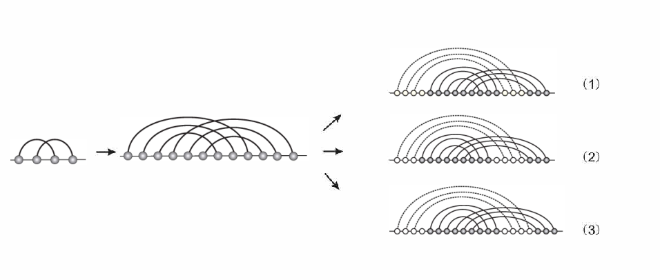
Refer to caption

Figure 4.5: Step I: a skeleton-shape (left) is inflated to a 33-noncrossing, canonical diagram. First, every arc in the skeleton-shape is inflated to a stack of size at least three (middle), and then the skeleton-shape is inflated to a new 33-noncrossing, canonical skeleton structure (right) by adding one stack of size three. There are three ways to insert the intervals isolated vertices.

Note that during this first inflation step no intervals of isolated vertices, other than those necessary for separating the nested stacks are inserted. We generate

  • •

    isolated segments i.e. sequences of isolated vertices ℒ=Seq​(𝒵)\mathcal{L}=\textsc{Seq}(\mathcal{Z}) with the generating function

    𝐋⁡(z)\displaystyle{\bf L}(z) =\displaystyle= 11−z\displaystyle\frac{1}{1-z}
  • •

    stacks, i.e. pairs consisting of the minimal sequence of arcs ℛσ\mathcal{R}^{\sigma} and an arbitrary extension consisting of arcs of arbitrary finite length

    𝒦3=𝒜3×Seq​(𝒜)\mathcal{K}^{3}=\mathcal{A}^{3}\times\textsc{Seq}\left(\mathcal{A}\right)

    with the generating function

    𝐊3​(z)\displaystyle\mathbf{K}^{3}(z) =\displaystyle= z6⋅11−z2\displaystyle z^{6}\cdot\frac{1}{1-z^{2}}
  • •

    induced stacks, i.e. stacks together with at least one nonempty interval of isolated vertices on either or both its sides.

    𝒩3=𝒦3×(𝒵×ℒ+𝒵×ℒ+(𝒵×ℒ)2),\mathcal{N}^{3}=\mathcal{K}^{3}\times\left(\mathcal{Z}\times\mathcal{L}+\mathcal{Z}\times\mathcal{L}+\left(\mathcal{Z}\times\mathcal{L}\right)^{2}\right),

    with the generating function

    𝐍3​(z)=z61−z2​(2​z1−z+(z1−z)2)\mathbf{N}^{3}(z)=\frac{z^{6}}{1-z^{2}}\left(2\frac{z}{1-z}+\left(\frac{z}{1-z}\right)^{2}\right)
  • •

    stems, that is pairs consisting of stacks 𝒦3\mathcal{K}^{3} and an arbitrarily long sequence of induced stacks

    ℳ3=𝒦3×Seq​(𝒩3),\mathcal{M}^{3}=\mathcal{K}^{3}\times\textsc{Seq}\left(\mathcal{N}^{3}\right),

    with the generating function

    𝐌3​(z)=𝐊3​(z)1−𝐍3​(z)=z61−z21−z61−z2​(2​z1−z+(z1−z)2).\displaystyle\mathbf{M}^{3}(z)=\frac{\mathbf{K}^{3}(z)}{1-\mathbf{N}^{3}(z)}=\frac{\frac{z^{6}}{1-z^{2}}}{1-\frac{z^{6}}{1-z^{2}}\left(2\frac{z}{1-z}+\left(\frac{z}{1-z}\right)^{2}\right)}.

Step II: here we insert additional isolated vertices at the remaining (2​h−1)(2h-1) positions, see Fig. 4.6.

Figure 4.6: Step II: the diagram (left) obtained in (1) in Fig. 4.5 is inflated to a new 33-noncrossing, canonical skeleton diagram (right) by adding isolated vertices (hollow discs).

Formally the second inflation is expressed via

  • •

    𝒥=ℒ2​h−1\mathcal{J}=\mathcal{L}^{2h-1}, where

    𝐉⁡(z)\displaystyle\mathbf{J}(z) =\displaystyle= (11−z)2​h−1\displaystyle\left(\frac{1}{1-z}\right)^{2h-1}

Combining Step I and Step II we arrive at

𝒮γ\displaystyle\mathcal{S}_{\gamma} =\displaystyle= (ℳ3)h×ℒ2​h−1\displaystyle\left(\mathcal{M}^{3}\right)^{h}\times\mathcal{L}^{2h-1} (4.3.15)

and accordingly

𝐒γ​(z)\displaystyle{\bf S}_{\gamma}(z) =\displaystyle= (z61−z21−z61−z2​(2​z1−z+(z1−z)2))h​(11−z)2​h−1\displaystyle\left(\frac{\frac{z^{6}}{1-z^{2}}}{1-\frac{z^{6}}{1-z^{2}}\left(2\frac{z}{1-z}+\left(\frac{z}{1-z}\right)^{2}\right)}\right)^{h}\left(\frac{1}{1-z}\right)^{2h-1} (4.3.16)
=\displaystyle= (1−z)​(z6(1−z2)​(1−z)2−(2​z−z2)​z6)h\displaystyle(1-z)\left(\frac{z^{6}}{(1-z^{2})(1-z)^{2}-(2z-z^{2})z^{6}}\right)^{h}
=\displaystyle= (1−z)​(z61−2​z+2​z3−z4−2​z7+z8)h.\displaystyle(1-z)\left(z^{6}\over{1-2z+2z^{3}-z^{4}-2z^{7}+z^{8}}\right)^{h}.

Since for any γ,γ1∈ℐ​𝒮​(h)\gamma,\gamma_{1}\in\mathcal{IS}(h) we have 𝐒γ​(z)=𝐒γ1​(z)\mathbf{S}_{\gamma}(z)=\mathbf{S}_{\gamma_{1}}(z), we derive

𝐒3[4]​(z)=∑h≥2∑γ∈ℐ​S​(m)𝐒γ​(z)=∑h≥2𝖨𝖲⁡(h)​𝐒γ​(z).{\bf S}^{[4]}_{3}(z)=\sum_{h\geq 2}\sum_{\gamma\in\,{\mathcal{I}S}(m)}\mathbf{S}_{\gamma}(z)=\sum_{h\geq 2}{\sf IS}(h)\mathbf{S}_{\gamma}(z).

Setting

η3​(z)=z61−2​z+2​z3−z4−2​z7+z8,\eta_{3}(z)={z^{6}\over{1-2z+2z^{3}-z^{4}-2z^{7}+z^{8}}}, (4.3.17)

we have, according to eq. (4.3.14) and Theorem 3.1 the following situation

𝐒3[4]​(z)\displaystyle{\bf S}^{[4]}_{3}(z) =\displaystyle= ∑h≥2𝖨𝖲⁡(h)​𝐒γ​(z)\displaystyle\sum_{h\geq 2}{\sf IS}(h)\,{\bf S}_{\gamma}(z) (4.3.18)
=\displaystyle= (1−z)​∑h≥2𝖨𝖲⁡(h)​(z61−2​z+2​z3−z4−2​z7+z8)h\displaystyle(1-z)\sum_{h\geq 2}{\sf IS}(h)\,\left(z^{6}\over{1-2z+2z^{3}-z^{4}-2z^{7}+z^{8}}\right)^{h}
=\displaystyle= (1−z)​𝐈𝐒​(z61−2​z+2​z3−z4−2​z7+z8),\displaystyle(1-z)\,{\bf IS}\left(z^{6}\over{1-2z+2z^{3}-z^{4}-2z^{7}+z^{8}}\right),

Claim 2 is proved.

Now we substitute eq. (4.3.9) into eq. (4.3.12), we arrive at eq. (4.3.8), where w0​(z)=z41−z2+z6w_{0}(z)={z^{4}\over{1-z^{2}+z^{6}}}. The theorem follows.


4.4 Asymptotic analysis

Denote y=z​𝐅32​(z)y=z{\bf F}_{3}^{2}(z), then we have

𝐒​(y)=𝐅3​(z).{\bf S}(y)={\bf F}_{3}(z). (4.4.19)

We will use singularity analysis to analyze the asymptotic behavior of the coefficients of 𝐒⁡(y){\bf S}(y). To apply singularity analysis to 𝐒⁡(y){\bf S}(y), we need to know its radius of convergence RR, the behavior of 𝐒⁡(y){\bf S}(y) near y=Ry=R, the absence of other singularities of 𝐒{\bf S} on the circle of convergence, Δ\Delta-analyticity of 𝐒⁡(y){\bf S}(y) and the singular expansion of 𝐒⁡(y){\bf S}(y). This information must be deduced from eq. (4.4.19) and a knowledge of 𝐅3{\bf F}_{3}. As is typical, we will see that 𝐅3{\bf F}_{3} has a unique singularity. This information is then transferred to 𝐒{\bf S} via eq. (4.4.19), then singularity analysis applies.

Lemma 4.5 (Existence and uniqueness of dominant singularity of 𝐒⁡(y){\bf S}(y)).

The dominant singularity of the generating function 𝐒⁡(y){\bf S}(y) is R=ρ​𝐅32​(ρ)≈0.0729R=\rho{\bf F}_{3}^{2}(\rho)\approx 0.0729, ρ=1/16\rho=1/16, and 𝐒⁡(y){\bf S}(y) has no singularity other from the circle of {y∣|y|=R}\{y\mid|y|=R\}, that is, 𝐒⁡(y){\bf S}(y) is analytically continuable around any y≠ρy\neq\rho with |y|≤R|y|\leq R.

Proof.

Claim 1. The radius of convergence, RR, is equal to ρ​𝐅32​(ρ)\rho{\bf F}^{2}_{3}(\rho), where ρ\rho is the radius of convergence of 𝐅3{\bf F}_{3}.

Since series 𝐒⁡(y){\bf S}(y) has nonnegative coefficients, we know that 𝐒⁡(y){\bf S}(y) has a radius of convergence of RR. since 𝐅3{\bf F}_{3} has nonnegative coefficients, d​y/d​z>0\text{d}y/\text{d}z>0 for 0<z<ρ0<z<\rho and so zz is an analytic function of yy for 0<y<R0<y<R. We now show that y=ρ​𝐅32​(ρ)y=\rho{\bf F}_{3}^{2}(\rho) is a singularity of 𝐒{\bf S}, from which R=ρ​𝐅32​(ρ)R=\rho{\bf F}_{3}^{2}(\rho) follows.

From Proposition 2.14, we know that 𝐅3​(ρ){\bf F}_{3}(\rho), 𝐅3′​(ρ){\bf F}_{3}^{\prime}(\rho), 𝐅3′′​(ρ){\bf F}_{3}^{\prime\prime}(\rho), 𝐅3′′′​(ρ){\bf F}_{3}^{\prime\prime\prime}(\rho) exist and are positive but 𝐅3(4)​(z)→∞{\bf F}_{3}^{(4)}(z)\rightarrow\infty as z→ρz\rightarrow\rho. From eq. (4.4.19),

𝐒(4)​(z​𝐅32​(z))=U⁡(𝐅3,𝐅3′,𝐅3′′,𝐅3′′′)​𝐅3(4)​(z)+V⁡(𝐅3,𝐅3′,𝐅3′′,𝐅3′′′)[𝐅3​(z)​(𝐅3​(z)+2​z​𝐅3′​(z))]7,{\bf S}^{(4)}(z{\bf F}_{3}^{2}(z))=\frac{U({\bf F}_{3},{\bf F}_{3}^{\prime},{\bf F}_{3}^{\prime\prime},{\bf F}_{3}^{\prime\prime\prime}){\bf F}_{3}^{(4)}(z)+V({\bf F}_{3},{\bf F}_{3}^{\prime},{\bf F}_{3}^{\prime\prime},{\bf F}_{3}^{\prime\prime\prime})}{[{\bf F}_{3}(z)({\bf F}_{3}(z)+2z{\bf F}_{3}^{\prime}(z))]^{7}}, (4.4.20)

where UU and VV are both multi-variable polynomials and U|z=ρ>0U|_{z=\rho}>0.

Thus 𝐒(4)​(y)→∞{\bf S}^{(4)}(y)\rightarrow\infty as y→(ρ​𝐅32​(ρ))−y\rightarrow(\rho{\bf F}^{2}_{3}(\rho))^{-} and so R=ρ​𝐅32​(ρ)R=\rho{\bf F}_{3}^{2}(\rho).

Claim 2. There are no other singularities of 𝐒⁡(y){\bf S}(y) existed on the circle of convergence |y|=R|y|=R.

By eq. (4.4.19), singularities of 𝐒⁡(y){\bf S}(y) are due to singularities of 𝐅3{\bf F}_{3} and values of yy near which inverting y=z​𝐅32​(z)y=z{\bf F}_{3}^{2}(z) uniquely is impossible.

Let us consider singularities of 𝐅3​(z){\bf F}_{3}(z). We have known that 𝐅3​(z){\bf F}_{3}(z) is Δ\Delta-analytic and its dominant singularity is ρ\rho and unique. Then let us consider inverting y=z​𝐅32​(z)y=z{\bf F}_{3}^{2}(z) on |y|=R|y|=R with y≠Ry\neq R. Thus z≠ρz\neq\rho and so 𝐅3{\bf F}_{3} is defined. By the implicit function theorem any singularities must be due to d​y/d​z=0\text{d}y/\text{d}z=0. We now use 𝐒′​(R)≠∞{\bf S}^{\prime}(R)\neq\infty. Since 𝐒⁡(y){\bf S}(y) has nonnegative coefficients, no singularity on |y|=R|y|=R can dominate y=Ry=R and so 𝐒′​(y)≠∞{\bf S}^{\prime}(y)\neq\infty on |y|=R|y|=R. By eq. (4.4.19),

𝐒′​(y)=d​𝐒d​y=d​𝐅3d​z/d​yd​z.{\bf S}^{\prime}(y)=\frac{\text{d}{\bf S}}{\text{d}y}=\frac{\text{d}{\bf F}_{3}}{\text{d}z}\bigg/\frac{\text{d}y}{\text{d}z}.

At a singularity, d​y/d​z=0\text{d}y/\text{d}z=0 and so 𝐅3′=0{\bf F}_{3}^{\prime}=0. Since d​y/d​z=𝐅32+2​z​𝐅3​𝐅3′\text{d}y/\text{d}z={\bf F}_{3}^{2}+2z{\bf F}_{3}{\bf F}_{3}^{\prime}, 𝐅3=0{\bf F}_{3}=0. If y=σ≠Ry=\sigma\neq R is a singularity with |σ|=R|\sigma|=R and rr is the corresponding value of zz, we have shown that 𝐒⁡(y)=𝐅3​(z)=(z−r)k​g​(z){\bf S}(y)={\bf F}_{3}(z)=(z-r)^{k}g(z) where k≥1k\geq 1, g⁡(r)≠0g(r)\neq 0 and gg is analytic near rr. Such rr is existed, which means rr is in the analytic domain of 𝐅3​(z){\bf F}_{3}(z), ℂ\[1/16,∞)\mathbb{C}\backslash[1/16,\infty), due to eq. (2.3.24). The proof is following:

From eq. (4.4.19), we derive the following equation,

z​𝐅32​(z)=z​𝐒2​(z​𝐅32​(z)),z{\bf F}^{2}_{3}(z)=z{\bf S}^{2}(z{\bf F}_{3}^{2}(z)),

then we have

z=y𝐒2​(y)z=\frac{y}{{\bf S}^{2}(y)} (4.4.21)

and

𝐒⁡(y)=𝐅3​(y​𝐒−2​(y)).{\bf S}(y)={\bf F}_{3}(y{\bf S}^{-2}(y)). (4.4.22)

Therefore, from eq. (4.4.21), we know that for any given σ≠R\sigma\neq R on the circle of |y|=R|y|=R, we have corresponding value of zz, rr, which is σ𝐒2​(σ)\frac{\sigma}{{\bf S}^{2}(\sigma)}. 𝐒2​(σ){\bf S}^{2}(\sigma) cannot be zero, or else, |z||z| will be infinity, then by eq. (4.4.21) and eq. (4.4.22) we have lim|z|→∞y⁡(z)=limy→σy𝐒2​(y)​𝐅32​(y𝐒2​(y))=σ\lim_{|z|\rightarrow\infty}y(z)=\lim_{y\rightarrow\sigma}\frac{y}{{\bf S}^{2}(y)}{\bf F}_{3}^{2}\left(\frac{y}{{\bf S}^{2}(y)}\right)=\sigma. But lim|z|→∞|y⁡(z)|>1.83>R\lim_{|z|\rightarrow\infty}|y(z)|>1.83>R, it is contradicted to |σ|=R|\sigma|=R. Hence rr cannot be infinity. Moreover, if rr lies on the line of [1/16,∞)[1/16,\infty), we have |r​𝐅32​(r)|=|σ|=R|r{\bf F}^{2}_{3}(r)|=|\sigma|=R. However, by the rigorous calculation of Mathematica, when r∈(1/16,1/8)r\in(1/16,1/8),

r​𝐅32​(r)=(1/16)​𝐅32​(1/16)+Ξ⁡(r)​(r−1/16),r{\bf F}^{2}_{3}(r)=(1/16){\bf F}^{2}_{3}(1/16)+\Xi(r)(r-1/16),

where Ξ⁡(r)\Xi(r) satisfying |Ξ⁡(r)|>0|\Xi(r)|>0 and |arg⁡Ξ⁡(r)|<0.19|\arg\Xi(r)|<0.19. Besides, min⁡|r​𝐅32​(r)|>0.12>(1/16)​𝐅32​(1/16)\min|r{\bf F}^{2}_{3}(r)|>0.12>(1/16){\bf F}^{2}_{3}(1/16) when r>1/8−1/32r>1/8-1/32. The two calculation results immediately imply that minr≥1/16⁡|r​𝐅32​(r)|=(1/16)​𝐅32​(1/16)=R\min_{r\geq 1/16}|r{\bf F}^{2}_{3}(r)|=(1/16){\bf F}^{2}_{3}(1/16)=R and the minimum arrives if and only if r=1/16r=1/16. Such case is contradicted to |σ|=R|\sigma|=R and σ≠R\sigma\neq R. Now we have proved the existence of rr.

Let us continue the main proof. Since

𝐒′​(y)=d​𝐅3/d​zd​(z​𝐅32)/d​z=(z−r)k−1(z−r)2​k−1​f​(z),{\bf S}^{\prime}(y)=\frac{\text{d}{\bf F}_{3}/\text{d}z}{\text{d}(z{\bf F}_{3}^{2})/\text{d}z}=\frac{(z-r)^{k-1}}{(z-r)^{2k-1}}f(z),

where f⁡(r)≠0f(r)\neq 0. This gives 𝐒′​(σ)=∞{\bf S}^{\prime}(\sigma)=\infty, a contradiction. Hence no such singularity σ\sigma exists, Claim 2 follows.

 
Lemma 4.6 (Δ\Delta-analytic continuation of 𝐒⁡(y){\bf S}(y)).

𝐒⁡(y){\bf S}(y) can be analytically continued to a Δ\Delta-domain at the singularity of RR.

Proof.

Claim 1. 𝐒⁡(y){\bf S}(y) is analytic in a “Δ\Delta-neighborhood” for RR, of the form

{|y−R|<δ′,arg⁡(y−R)∈(ϕ,2​π−ϕ)},\{|y-R|<\delta^{\prime},\arg(y-R)\in(\phi,2\pi-\phi)\},

with δ′>0\delta^{\prime}>0 and 0<ϕ<π/20<\phi<\pi/2.

First, by Fusy’s method [8], the singular expansion of 𝐒⁡(y){\bf S}(y) at RR holds in a neighborhood Ω\Omega of RR, where Ω\Omega is the image of y⁡(z)y(z) mapping from a slit neighborhood Θ\Theta, which is defined by {|z−ρ|<δ}\{|arg(z−ρ)|≤ϕ′}\{|z-\rho|<\delta\}\backslash\{|\arg(z-\rho)|\leq\phi^{\prime}\}, with δ>0\delta>0 and 0<ϕ′<π/20<\phi^{\prime}<\pi/2. Since y′​(z)y^{\prime}(z) converges to a positive constant at z=ρz=\rho, it is locally conformal at ρ\rho. Hence Ω\Omega contains a “Δ\Delta-neighborhood” for RR, of the form

N⁡(Δ)≡{|y−R|<δ′,arg​(y−R)∈(ϕ,2​π−ϕ)},N(\Delta)\equiv\{|y-R|<\delta^{\prime},\text{arg}(y-R)\in(\phi,2\pi-\phi)\}, (4.4.23)

with δ′>0\delta^{\prime}>0 and 0<ϕ<π/20<\phi<\pi/2.

Second, The claim that y⁡(z)y(z) is univalent (bijective and analytic) in N⁡(Δ)N(\Delta), is true. Since y′​(ρ)>0y^{\prime}(\rho)>0, by Noshiro-Warschawski Theorem [9], we know that y⁡(z)y(z) is respectively univalent in Θ∩{Imz>0}\Theta\cap\{\text{Im}z>0\} and Θ∩{Imz<0}\Theta\cap\{\text{Im}z<0\} when zz is in some neighborhood of ρ\rho. Due to 𝐅3​(z){\bf F}_{3}(z), yy has a singular expansion,

y⁡(z)=R+y′​(ρ)​(z−ρ)+o⁡(z−ρ)y(z)=R+y^{\prime}(\rho)(z-\rho)+o(z-\rho)

around ρ\rho. Assuming δ\delta in eq. (4.4.23) has been chosen sufficiently small enough making |z|<ρ|z|<\rho when |arg⁡(z−ρ)|>2​π3|\arg(z-\rho)|>\frac{2\pi}{3}, and

arg⁡(y⁡(z)−R)∈(0,π),\arg(y(z)-R)\in(0,\pi), (4.4.24)

when arg⁡(z−ρ)∈(ϕ′,2​π3]\arg(z-\rho)\in(\phi^{\prime},\frac{2\pi}{3}] , concluded by the same method for eq.(2.4.45).

For the point z∈Θz\in\Theta of arg⁡(z−ρ)∈(2​π3,π)\arg(z-\rho)\in(\frac{2\pi}{3},\pi). We draw a straight line {s(t)∣s(0)=z,s(1)=z0,0≤t≤1}\{s(t)\mid s(0)=z,s(1)=z_{0},0\leq t\leq 1\}, where z0z_{0} satisfies z0∈Θz_{0}\in\Theta and arg⁡(z0−ρ)=2​π3\arg(z_{0}-\rho)=\frac{2\pi}{3}. Clearly y⁡(z0)y(z_{0}) is in the upper-half plain. Suppose zz maps to the lower-half plain. The smooth curve of y⁡(s⁡(t))y(s(t)) must intersect the line of [0,R][0,R], which means there exists t0t_{0} such that y⁡(s⁡(t0))=r0y(s(t_{0}))=r_{0}, 0≤r0≤R0\leq r_{0}\leq R. Using eq. (4.4.21) we solute that s⁡(t0)=r0/𝐒2​(r0)s(t_{0})=r_{0}/{\bf S}^{2}(r_{0}), which implies s⁡(t0)s(t_{0}) is real. It is impossible since the line of {s⁡(t)}\{s(t)\} cannot touch the real axis due to the convexity of Θ∩{Imz>0}\Theta\cap\{\text{Im}z>0\}. Therefore,

y⁡(z)∈{z∣Im​z>0},when z∈Θ and arg⁡(z−ρ)∈(2​π3,π).y(z)\in\{z\mid\text{Im}z>0\},\text{when $z\in\Theta$ and $\arg(z-\rho)\in(\frac{2\pi}{3},\pi)$}. (4.4.25)

Eq. (4.4.24) and eq. (4.4.25) will lead us that y⁡(z)y(z) is mapping Θ∩{Imz>0}\Theta\cap\{\text{Im}z>0\} to a upper-half plain. By the symmetric theorem for analytic function [4], y⁡(z)y(z) is mapping Θ∩{Imz<0}\Theta\cap\{\text{Im}z<0\} to a lower-half plain as well. Obviously, y⁡(z)y(z) is strictly monotonic increasing on the real segment of [0,ρ][0,\rho] and y⁡([0,ρ])=[0,R]y([0,\rho])=[0,R], hence y⁡(z)y(z) is globally univalent in the whole Θ\Theta.

According to eq. (4.4.19), the analyticity of inversion function of y⁡(z)y(z) and 𝐅3{\bf F}_{3} respectively in “Δ\Delta-neighborhood” N⁡(Δ)N(\Delta) and Θ\Theta imply the truth of Claim 1.

Figure 4.7: The construction of Δ\Delta-domain for 𝐒⁡(y){\bf S}(y): the dark grey part is the analytic continuous domain based on the disc of U⁡(0,R)U(0,R) (light grey). The dash line is the edge of Δ\Delta-domain which is contained in the whole analytic domain (dark and light grey) of 𝐒⁡(y){\bf S}(y).

Claim 2. 𝐒⁡(y){\bf S}(y) can be analytically continued to a Δ\Delta-domain at the singularity of RR.

The previous claim actually tells us 𝐒⁡(y){\bf S}(y) can be analytically continued to a “Δ\Delta-neighborhood” domain N⁡(Δ)N(\Delta), whose boundary makes an acute angle with the half line ℝ≥R\mathbb{R}_{\geq R}.

Claim 2 of Lemma 4.5 reveals that for any y′y^{\prime} on the circle of |y|=R|y|=R outside N⁡(Δ)N(\Delta), 𝐒{\bf S} can be analytically continued to U⁡(y′,δy′)U(y^{\prime},\delta_{y^{\prime}}) which contains in an image of y⁡(z)y(z) univalently mapping from a neighborhood U⁡(r,ε)U(r,\varepsilon) where y⁡(r)=y′y(r)=y^{\prime}. For the reason that {y∣|y|=R}\{y\mid|y|=R\} without containing in N⁡(Δ)N(\Delta) is a closed curve ℓ\ell, we can find a finite neighborhoods, {U⁡(yi,δyi)}1≤i≤n⊂{U⁡(y′,δy′)}|y′|=R\{U(y_{i},\delta_{y_{i}})\}_{1\leq i\leq n}\subset\{U(y^{\prime},\delta_{y^{\prime}})\}_{|y^{\prime}|=R}, covering ℓ\ell. Since

U⁡(yi,δyi)∩U⁡(yi+1,δyi+1)∩U⁡(0,R)≠∅,1≤i≤n−1,U(y_{i},\delta_{y_{i}})\cap U(y_{i+1},\delta_{y_{i+1}})\cap U(0,R)\neq\emptyset,\quad 1\leq i\leq n-1,

we have that ∪i=1nU(yi,δyi)\cup^{n}_{i=1}U(y_{i},\delta_{y_{i}}) is an analytic continuation domain for 𝐒⁡(y){\bf S}(y).

Combining these two facts and

⋃i=1nU⁡(yi,δyi)∩U⁡(0,R)∩N⁡(Δ)≠∅,\bigcup^{n}_{i=1}U(y_{i},\delta_{y_{i}})\cap U(0,R)\cap N(\Delta)\neq\emptyset,

we obtain a new analytic continuation domain for 𝐒⁡(y){\bf S}(y), see Fig. 4.7. Using the method of Step (c) in Proposition 2.10, we are able to find a Δ\Delta-domain inside, which means we have proved 𝐒⁡(y){\bf S}(y) is Δ\Delta-analytic. Here the whole proof is complete.

 
Lemma 4.7 (Singular expansion of 𝐒⁡(y){\bf S}(y)).

The singular expansion of 𝐒⁡(y){\bf S}(y) for y→Ry\rightarrow R is given by

𝐒⁡(y)=∑i=04bi​(y−R)i+c′​(y−R)4​log⁡(y−R)+o⁡((y−R)4){\bf S}(y)=\sum_{i=0}^{4}b_{i}(y-R)^{i}+c^{\prime}(y-R)^{4}\log(y-R)+o((y-R)^{4}) (4.4.26)

were c′c^{\prime} is some negative constant, and bi=1i!​𝐒(i)​(R−)b_{i}=\frac{1}{i!}{\bf S}^{(i)}(R^{-}), 0≤i≤30\leq i\leq 3.

Proof.

Claim 1. The singular expansion of 𝐒⁡(y){\bf S}(y) for y→Ry\rightarrow R is given by

𝐒⁡(y)=∑i=03bi​(y−R)i+(y−R)4​log⁡(y−R)​(c′+o⁡(1)).{\bf S}(y)=\sum_{i=0}^{3}b_{i}(y-R)^{i}+(y-R)^{4}\log(y-R)\left(c^{\prime}+o(1)\right). (4.4.27)

Furthermore, c′c^{\prime} is some constant, and bi=1i!​𝐒(i)​(R−)b_{i}=\frac{1}{i!}{\bf S}^{(i)}(R^{-}), 0≤i≤30\leq i\leq 3.

Since 𝐅3(m)​(ρ−){\bf F}_{3}^{(m)}(\rho^{-}), 0≤m≤30\leq m\leq 3 exists, y(m)​(ρ−)y^{(m)}(\rho^{-}) exists. Therefore 𝐒(m)​(R−){\bf S}^{(m)}(R^{-}) exists. Then we set

E⁡(y)=𝐒⁡(y)−∑i=03bi​(y−R)i,E(y)={\bf S}(y)-\sum_{i=0}^{3}b_{i}(y-R)^{i}, (4.4.28)

where bi=1i!​𝐒(i)​(R−)b_{i}=\frac{1}{i!}{\bf S}^{(i)}(R^{-}), 0≤i≤30\leq i\leq 3.

Furthermore, by eq. (2.5.60), we have the singular expansion of y⁡(z)y(z) which is

y⁡(z)=∑i=03ai​(z−ρ)i+c3′′​(z−ρ)4​log⁡(z−ρ)​(1+o⁡(1))y(z)=\sum_{i=0}^{3}a_{i}(z-\rho)^{i}+c_{3}^{\prime\prime}(z-\rho)^{4}\log(z-\rho)\left(1+o(1)\right)

where c3′′c_{3}^{\prime\prime} is some negative constant, and ai=1i!​y(i)​(ρ−)a_{i}=\frac{1}{i!}y^{(i)}(\rho^{-}), 0≤i≤30\leq i\leq 3.

Now we begin to discuss the higher term of the expansion of 𝐒⁡(y){\bf S}(y).

By eq. (4.4.28), we know that

𝐅3​(z)=𝐒⁡(y⁡(z))\displaystyle{\bf F}_{3}(z)={\bf S}(y(z)) =∑i=03bi​(y⁡(z)−y⁡(ρ))i+E⁡(y⁡(z))\displaystyle=\sum_{i=0}^{3}b_{i}(y(z)-y(\rho))^{i}+E(y(z))
=∑i=03bi​[∑j=13aj​(z−ρ)j+c3′​(z−ρ)4​log⁡(z−ρ)​(1+o⁡(1))]i\displaystyle=\sum_{i=0}^{3}b_{i}\left[\sum_{j=1}^{3}a_{j}(z-\rho)^{j}+c_{3}^{\prime}(z-\rho)^{4}\log(z-\rho)(1+o(1))\right]^{i}
+E⁡(y⁡(z)).\displaystyle+E(y(z)). (4.4.29)

From Proposition 2.14 and Faà di Bruno’s Formula [40], for 1≤m≤31\leq m\leq 3 we have

1m!​𝐅3(m)​(ρ−)\displaystyle\frac{1}{m!}{\bf F}_{3}^{(m)}(\rho^{-}) =∑i=0m∑t1+t2+⋯+tm=it1+2​t2+⋯+m​tm=m1t1!t2!⋯tm!​𝐒(i)​(R−)​∏j=1m(y(j)​(ρ−)j!)tj\displaystyle=\sum_{i=0}^{m}\sum_{t_{1}+t_{2}+\cdots+t_{m}=i\atop t_{1}+2t_{2}+\cdots+mt_{m}=m}\frac{1}{t_{1}!t_{2}!\cdots t_{m}!}{\bf S}^{(i)}(R^{-})\prod_{j=1}^{m}\left(\frac{y^{(j)}(\rho^{-})}{j!}\right)^{t_{j}}
=∑i=0m1i!​𝐒(i)​(R−)​[(z−ρ)m]​(∑j=1my(j)​(ρ−)j!​(z−ρ)j)i\displaystyle=\sum_{i=0}^{m}\frac{1}{i!}{\bf S}^{(i)}(R^{-})[(z-\rho)^{m}]\left(\sum_{j=1}^{m}\frac{y^{(j)}(\rho^{-})}{j!}(z-\rho)^{j}\right)^{i}
=∑i=0mbi​[(z−ρ)m]​(∑j=1maj​(z−ρ)j)i.\displaystyle=\sum_{i=0}^{m}b_{i}[(z-\rho)^{m}]\left(\sum_{j=1}^{m}a_{j}(z-\rho)^{j}\right)^{i}. (4.4.30)

So by Eq. (4.4.30) and 𝐅3​(ρ−)=𝐒⁡(R−)=b0{\bf F}_{3}(\rho^{-})={\bf S}(R^{-})=b_{0}, it leads that the every coefficient of (z−ρ)m(z-\rho)^{m}, 0≤m≤30\leq m\leq 3 in the expansion of each side in eq. (4.4.29) is eliminated. Therefore we have

(z−ρ)4​log⁡(z−ρ)​(c′′+o⁡(1))=E⁡(y⁡(z)),(z-\rho)^{4}\log(z-\rho)(c^{\prime\prime}+o(1))=E(y(z)), (4.4.31)

where c′′c^{\prime\prime} is some constant.

We divide E⁡(y)E(y) by (y−R)4​log⁡(y−R)(y-R)^{4}\log(y-R) and then

limy→RE⁡(y)(y−R)4​log⁡(y−R)\displaystyle\lim_{y\rightarrow R}\frac{E(y)}{(y-R)^{4}\log(y-R)} =limz→ρE⁡(y⁡(z))(y⁡(z)−y⁡(ρ))4​log⁡(y⁡(z)−y⁡(ρ))\displaystyle=\lim_{z\rightarrow\rho}\frac{E(y(z))}{(y(z)-y(\rho))^{4}\log(y(z)-y(\rho))}
=limz→ρ(z−ρ)4​log⁡(z−ρ)​(c′′+o⁡(1))(y⁡(z)−y⁡(ρ))4​log⁡(y⁡(z)−y⁡(ρ))\displaystyle=\lim_{z\rightarrow\rho}\frac{(z-\rho)^{4}\log(z-\rho)(c^{\prime\prime}+o(1))}{(y(z)-y(\rho))^{4}\log(y(z)-y(\rho))}
=a constant,\displaystyle=\text{a constant}, (4.4.32)

since z−ρy⁡(z)−y⁡(ρ)\frac{z-\rho}{y(z)-y(\rho)} and log⁡(z−ρ)log⁡(y⁡(z)−y⁡(ρ))\frac{\log(z-\rho)}{\log(y(z)-y(\rho))} both exist as z→ρz\rightarrow\rho. Therefore

𝐒⁡(y)=∑i=03bi​(y−R)i+(y−R)4​log⁡(y−R)​(c′+o⁡(1)),{\bf S}(y)=\sum_{i=0}^{3}b_{i}(y-R)^{i}+(y-R)^{4}\log(y-R)(c^{\prime}+o(1)), (4.4.33)

whence Claim 3.

Claim 2. c′c^{\prime} is negative.

From eq. (4.4.20) with T=𝐅3​(ρ−)+2​ρ​𝐅3′​(ρ−)T={\bf F}_{3}(\rho^{-})+2\rho{\bf F}^{\prime}_{3}(\rho^{-}) and F=𝐅3​(ρ−)F={\bf F}_{3}(\rho^{-}),

𝐒(4)​(y)∼K⋅𝐅3(4)​(z)/(F​T)7{\bf S}^{(4)}(y)\sim K\cdot{\bf F}_{3}^{(4)}(z)/(FT)^{7} (4.4.34)

as y→Ry\rightarrow R, where KK is a positive constant equaled U⁡(𝐅3,𝐅3′,𝐅3′′,𝐅3′′′)|z=ρ=F4​T2U({\bf F}_{3},{\bf F}^{\prime}_{3},{\bf F}^{\prime\prime}_{3},{\bf F}^{\prime\prime\prime}_{3})|_{z=\rho}=F^{4}T^{2}. From y=z​𝐅32​(z)y=z{\bf F}_{3}^{2}(z) we have

z−ρ∼(y−R)/(F​T).z-\rho\sim(y-R)/(FT). (4.4.35)

From eq. (2.5.60),

𝐅3(4)​(z)∼c3′​d4​[(z−ρ)4​log⁡(z−ρ)]d​z4=c3′​(4!​log⁡(z−ρ)+M),{\bf F}^{(4)}_{3}(z)\sim c^{\prime}_{3}\frac{\text{d}^{4}[(z-\rho)^{4}\log(z-\rho)]}{\text{d}z^{4}}=c^{\prime}_{3}(4!\log(z-\rho)+M), (4.4.36)

where MM is a positive integer.

Combining eq. (4.4.34)–(4.4.36) we obtain

𝐒(4)​(y)∼K⋅c3′(F​T)7​(4!​(log⁡(y−R)−log⁡(F​T))+M)∼K⋅c3′(F​T)7​d4​[(y−R)4​log⁡(y−R)]d​y4.{\bf S}^{(4)}(y)\sim\frac{K\cdot c^{\prime}_{3}}{(FT)^{7}}(4!(\log(y-R)-\log(FT))+M)\sim\frac{K\cdot c^{\prime}_{3}}{(FT)^{7}}\frac{\text{d}^{4}[(y-R)^{4}\log(y-R)]}{\text{d}y^{4}}. (4.4.37)

Differentiating eq. (4.4.27) four times and comparing to eq. (4.4.37), we know that

c′=K⋅c3′(F​T)7,c^{\prime}=\frac{K\cdot c^{\prime}_{3}}{(FT)^{7}}, (4.4.38)

which means c′c^{\prime} is negative, whence Claim 2. Based on the above claims, we do the final proof, we set

E′​(y)=𝐒⁡(y)−∑i=03bi​(y−R)i−c′​(y−R)4​log⁡(y−R),E^{\prime}(y)={\bf S}(y)-\sum_{i=0}^{3}b_{i}(y-R)^{i}-c^{\prime}(y-R)^{4}\log(y-R),

where Substituting y=z​𝐅32​(z)y=z{\bf F}^{2}_{3}(z) into the equation above, we have

E′​(y​(z))\displaystyle E^{\prime}(y(z)) =𝐅3​(z)−∑m=03bm​(y⁡(z)−R)m−c′​(y⁡(z)−R)4​log⁡(y⁡(z)−R)\displaystyle={\bf F}_{3}(z)-\sum_{m=0}^{3}b_{m}(y(z)-R)^{m}-c^{\prime}(y(z)-R)^{4}\log(y(z)-R)
=∑m=03[1m!​𝐅3(m)​(ρ−)−∑i=0mbi​[(z−ρ)m]​(∑j=1maj​(z−ρ)j)i]​(z−ρ)m\displaystyle=\sum_{m=0}^{3}\left[\frac{1}{m!}{\bf F}_{3}^{(m)}(\rho^{-})-\sum_{i=0}^{m}b_{i}[(z-\rho)^{m}]\left(\sum_{j=1}^{m}a_{j}(z-\rho)^{j}\right)^{i}\right](z-\rho)^{m}
+[c3′−c′​(F​T)4−2​b1​ρ​F​c3′]​log⁡(z−ρ)\displaystyle+\left[c^{\prime}_{3}-c^{\prime}(FT)^{4}-2b_{1}\rho Fc^{\prime}_{3}\right]\log(z-\rho)
+θ⁡((z−ρ)4),\displaystyle+\theta((z-\rho)^{4}), (4.4.39)

where g⁡(z)=θ⁡(f⁡(z))g(z)=\theta(f(z)) means limz→ρ|g⁡(z)/f⁡(z)|\lim_{z\rightarrow\rho}|g(z)/f(z)| is a positive constant. In the view of the equation of eq. (4.4.30), eq. (4.4.38) and b1=𝐅3′​(ρ)F​Tb_{1}=\frac{{\bf F}_{3}^{\prime}(\rho)}{FT}, we imply that the former two terms of eq. (4.4.39) are actually zero, which means

E′​(y⁡(z))=θ⁡((z−ρ)4).E^{\prime}(y(z))=\theta((z-\rho)^{4}).

Using the same deducting method of eq. (4.4.32), we have

E′​(y)=θ⁡((y−R)4)E^{\prime}(y)=\theta((y-R)^{4})

The proof is complete.  

Currently, we have the Δ\Delta-analytic property and the singular expansion of 𝐒⁡(y){\bf S}(y). The finale is applying the transfer rule (Corollary 2.8) which yields directly the following asymptotic estimate for the number of 33-noncrossing skeleton matching.

Theorem 4.8 (Asymptotic number of skeleton matching).

The asymptotic behavior of the number of 33-noncrossing skeleton matching with hh arcs is given by

𝖲⁡(h)∼C⋅h−5​R−h,{\sf S}(h)\ \sim\ C\cdot h^{-5}R^{-h},

where C≈3.03096C\approx 3.03096, see Fig. 4.8.

The multiplier CC is not estimated but precisely computed as follow with the help of eq. (4.4.20) and eq. (4.4.38),

C=−K​c3′(F​T)7⋅R4⋅4!=24​(−512+165​π)53125​(256−81​π)5​π.C=-\frac{Kc^{\prime}_{3}}{(FT)^{7}}\cdot R^{4}\cdot 4!=\frac{24(-512+165\pi)^{5}}{3125(256-81\pi)^{5}\pi}.
Theorem 4.9.

The number of canonical 33-noncrossing skeleton diagrams of length nn with arc length ≥4\geq 4, 𝖲3[4]​(n){\sf S}^{[4]}_{3}(n), has asymptotic of

𝖲3[4]​(n)∼C′​n−5​η−n,{\sf S}^{[4]}_{3}(n)\ \sim\ C^{\prime}n^{-5}\eta^{-n}, (4.4.40)

where C′≈7892.16C^{\prime}\approx 7892.16 and η≈0.4934\eta\approx 0.4934 is the minimal positive real solution of ϑ⁡(z)=R\vartheta(z)=R, where

ϑ⁡(z)=(w0​(z)​z1−z)2\vartheta(z)=\left({\sqrt{w_{0}(z)}z}\over{1-z}\right)^{2}

and w0​(z)=z41−z2+z6w_{0}(z)={z^{4}\over{1-z^{2}+z^{6}}}. See Fig. 4.8.

Proof.

Pringsheim’s Theorem [42] guarantees that 𝐒3[4]​(z){\bf S}^{[4]}_{3}(z) has a dominant real positive singularity η\eta. We verify that η\eta, which is the unique solution of minimum modulus of the equation ϑ⁡(z)=R\vartheta(z)=R, is the unique dominant singularity of 𝐒3[4]​(z){\bf S}^{[4]}_{3}(z), and ϑ′​(η)>0\vartheta^{\prime}(\eta)>0.

Here we discuss a claim that |ϑ⁡(z)||\vartheta(z)| is constraint in the closed disc with radius of RR when {|z|≤η}\{|z|\leq\eta\}. By maximum modulus theorem, we only need to focus on {|z|=η}\{|z|=\eta\}. Since

|ϑ⁡(z)|=η6|1−z|2​|1−z2+z6|.|\vartheta(z)|=\frac{\eta^{6}}{|1-z|^{2}|1-z^{2}+z^{6}|}. (4.4.41)

Studying each factor of the denominator of eq. (4.4.41) by replacing zz to η⁡(cos⁡x+i​sin⁡x)\eta(\cos x+\text{i}\sin x), we have the following functions corresponding to xx,

|1−z|2\displaystyle|1-z|^{2} =\displaystyle= 1−2​η​cos⁡x+η2,\displaystyle 1-2\eta\cos x+\eta^{2},
|1−z2+z6|2\displaystyle|1-z^{2}+z^{6}|^{2} =\displaystyle= 1+η4+η12−2​η2​cos⁡2​x−2​η8​cos⁡4​x+2​η6​cos⁡6​x.\displaystyle 1+\eta^{4}+\eta^{12}-2\eta^{2}\cos 2x-2\eta^{8}\cos 4x+2\eta^{6}\cos 6x.

Finding critical points for every function above and we can easily conclude that both functions reach the minimum when x=0x=0. Therefore the maximum of |ϑ⁡(z)||\vartheta(z)| for |z|=η|z|=\eta is |ϑ⁡(η)||\vartheta(\eta)|, which is also equal to RR, whence the claim.

Furthermore,

𝐆⁡(x)=𝐒⁡(x)−1−x,{\bf G}(x)={\bf S}(x)-1-x,

which means 𝐆⁡(x){\bf G}(x) has the same expansion formation as 𝐒⁡(x){\bf S}(x). According to Proposition 2.10 we therefore have

𝖲3[4]​(n)∼C′​n−5​(η−1)n.{\sf S}^{[4]}_{3}(n)\sim C^{\prime}\,n^{-5}\,(\eta^{-1})^{n}.

Here C′C^{\prime} can be precisely computed as follow,

C′=(1−η)⋅ϑ′​(η)4⋅820125​π7256​(256−81​π)5​(−512+165​π)3⋅4!⋅η4,C^{\prime}=(1-\eta)\cdot\vartheta^{\prime}(\eta)^{4}\cdot\frac{820125\pi^{7}}{256(256-81\pi)^{5}(-512+165\pi)^{3}}\cdot 4!\cdot\eta^{4},

which is concluded by eq. (4.3.8), eq. (4.4.27) and Corollary 2.8. The proof of Theorem 4.9 is complete.  

Figure 4.8: The computational experiment of asymptotic enumeration: The straight lines in both figures are y=Cy=C (left) and y=C′y=C^{\prime} (right) respectively. The curves are plotted by two lists of points, 𝖲⁡(n)/(n−5​R−n),n=1,…,500{\sf S}(n)/(n^{-5}R^{-n}),n=1,\ldots,500 (left) and 𝖲3[4]​(n)/(n−5​η−n),n=1,…,3000{\sf S}^{[4]}_{3}(n)/(n^{-5}\eta^{-n}),n=1,\ldots,3000 (right). We notice that each curve is well approaching the corresponding straight line, which means the asymptotic enumeration makes sense.

4.5 Discussion

So far, we have concluded the asymptotic properties of the number of 33-noncrossing skeleton matching and canonical diagrams with length nn. The two results solves the complexity problem of Huang’s folding algorithm [18], which means that we have had a strict mathematical way to inform how much time we cost in Huang’s algorithm. In this section we will make a exploration to the skeleton diagrams. First we are going to take a look at the statistics of arcs in canonical 33-noncrossing skeleton diagrams, then we prospect the further research to the asymptotic analysis for kk-noncrossing skeleton diagrams.

4.5.1 Statistics of arcs in canonical 33-noncrossing skeleton diagrams

In this section, we discuss the distribution of arcs in canonical kk-noncrossing skeleta with certain number of vertices. Let 𝔸n​(S)\mathbb{A}_{n}(S) denote the number of arcs in a 33-noncrossing skeleton diagrams, SS and let 𝒜⁡(n,h)\mathcal{A}(n,h) and A​(n,h)\textsf{A}(n,h) denote the set and number of canonical 33-noncrossing skeleton diagrams, having exactly hh arcs. Now we will study 𝔸n\mathbb{A}_{n}, where ℙ⁡(𝔸n=h)=A​(n,h)S3[4]​(n)\mathbb{P}(\mathbb{A}_{n}=h)=\frac{\textsf{A}(n,h)}{\textsf{S}_{3}^{[4]}(n)}.

To compute the distribution of 33-noncrossing skeleta diagrams, i.e. 𝔸n\mathbb{A}_{n}, the first step is to compute the bivariate generating function

𝐀⁡(z,u)=∑n≥0∑0≤h≤n2𝖠⁡(n,h)​uh​zn.{\bf A}(z,u)=\sum_{n\geq 0}\sum_{0\leq h\leq\frac{n}{2}}{\sf A}(n,h)\,u^{h}z^{n}.
Theorem 4.10.

Let uu and zz be indeterminants. Then we have the identity of formal power series

𝐀⁡(z,u)=(1−z)​𝐆​(w⁡(u,z)​z6(1−z)2),{\bf A}(z,u)=(1-z){\bf G}\left(\frac{w(u,z)z^{6}}{(1-z)^{2}}\right), (4.5.42)

where w⁡(u,z)w(u,z) is given by

w⁡(u,z)=u31−u​z2+u3​z6w(u,z)=\frac{u^{3}}{1-uz^{2}+u^{3}z^{6}}

and

𝐆⁡(x)=𝐒⁡(x)−1−x.{\bf G}(x)={\bf S}(x)-1-x.

Considered as a relation between analytic functions, eq. (4.5.42) holds for u=esu=\text{e}^{s} and |s|≤ε|s|\leq\varepsilon for ε\varepsilon sufficiently small and |z|≤12|z|\leq\frac{1}{2}.

Proof.

Let 𝒮3[4]​(γ,h,n)\mathcal{S}_{3}^{[4]}(\gamma,h,n) denote the set of canonical 33-noncrossing structures, having length nn and hh arcs, contained in the preimage of a fixed skeleton shape, γ∈ℐ​𝒮​(m)\gamma\in\mathcal{IS}(m). Then 𝒮3[4]=∪˙​ψ−1​(γ)\mathcal{S}_{3}^{[4]}=\dot{\cup}\psi^{-1}(\gamma) and ψ−1​(γ)=∪˙n​𝒮3[4]​(γ,h,n)\psi^{-1}(\gamma)=\dot{\cup}_{n}\mathcal{S}_{3}^{[4]}(\gamma,h,n) where ψ:𝒮3[4]→ℐ​𝒮\psi:\mathcal{S}_{3}^{[4]}\rightarrow\mathcal{IS} is the surjective projection into skeleton shape. Then

𝐀⁡(z,u)\displaystyle{\bf A}(z,u) =\displaystyle= ∑m≥0∑γ∈ℐ​S​(m)∑n,h|𝒮3[4]​(γ,h,n)|​zn​uh⏟𝐀γ​(z,u),\displaystyle\sum_{m\geq 0}\sum_{\gamma\in\,{\mathcal{I}S}(m)}\underbrace{\sum_{n,h}|\mathcal{S}_{3}^{[4]}(\gamma,h,n)|z^{n}u^{h}}_{\mathbf{A}_{\gamma}(z,u)},

where 𝐀γ​(z,u)\mathbf{A}_{\gamma}(z,u) is the bivariate generating function of 33-noncrossing canonical skeleton diagrams having the shape γ\gamma. A structure inflated from γ\gamma has ss stems and (2​s−1)(2s-1) intervals of isolated vertices. We build these structures in a modular way via the combinatorial classes ℳ\mathcal{M} (stems), 𝒦3\mathcal{K}^{3} (stacks), 𝒩3\mathcal{N}^{3} (induced stacks), ℒ\mathcal{L} (isolated vertices), ℛ\mathcal{R} (labelled arcs) and 𝒵\mathcal{Z} (vertices), where 𝐙⁡(z)=z\mathbf{Z}(z)=z and 𝐑⁡(z,u)=u​z2\mathbf{R}(z,u)=uz^{2}. We proceed in complete analogy to the proof of Theorem 4.4, in fact all we have to is to substitute 𝐑⁡(z,u)=u​z2\mathbf{R}(z,u)=uz^{2}, i.e. the bivariate generating function of labelled arcs for 𝐑⁡(z)=z2\mathbf{R}(z)=z^{2}. Accordingly we generate

  • •

    isolated segments i.e. sequences of isolated vertices ℒ=Seq​(𝒵)\mathcal{L}=\textsc{Seq}(\mathcal{Z}), with the generating function

    𝐋⁡(z)\displaystyle{\bf L}(z) =\displaystyle= 11−z\displaystyle\frac{1}{1-z}
  • •

    stacks , i.e. pairs consisting of the minimal sequence of arcs ℛ3\mathcal{R}^{3} and an arbitrary extension consisting of arcs of arbitrary finite length 𝒦3=ℛ3×Seq​(ℛ)\mathcal{K}^{3}=\mathcal{R}^{3}\times\textsc{Seq}\left(\mathcal{R}\right), with the generating function

    𝐊τ​(z,u)\displaystyle\mathbf{K}^{\tau}(z,u) =\displaystyle= (u​z2)31−u​z2\displaystyle\frac{(uz^{2})^{3}}{1-uz^{2}}
  • •

    induced stacks, i.e. stacks together with at least one nonempty interval of isolated vertices on either or both its sides

    𝒩3=𝒦3×(𝒵×ℒ+𝒵×ℒ+(𝒵×ℒ)2),\mathcal{N}^{3}=\mathcal{K}^{3}\times\left(\mathcal{Z}\times\mathcal{L}+\mathcal{Z}\times\mathcal{L}+\left(\mathcal{Z}\times\mathcal{L}\right)^{2}\right),

    with the generating function

    𝐍3​(z,u)=(u​z2)31−u​z2​(2​z1−z+(z1−z)2)\mathbf{N}^{3}(z,u)=\frac{(uz^{2})^{3}}{1-uz^{2}}\left(2\frac{z}{1-z}+\left(\frac{z}{1-z}\right)^{2}\right)
  • •

    stems that is pairs consisting of stacks 𝒦τ\mathcal{K}^{\tau} and an arbitrarily long sequence of induced stacks

    ℳ3=𝒦3×Seq​(𝒩3),\mathcal{M}^{3}=\mathcal{K}^{3}\times\textsc{Seq}\left(\mathcal{N}^{3}\right),

    with the generating function

    𝐌3​(z,u)=𝐊3​(z,u)1−𝐍3​(z,u)=(u​z2)31−u​z21−(u​z2)31−u​z2​(2​z1−z+(z1−z)2).\displaystyle\mathbf{M}^{3}(z,u)=\frac{\mathbf{K}^{3}(z,u)}{1-\mathbf{N}^{3}(z,u)}=\frac{\frac{(uz^{2})^{3}}{1-uz^{2}}}{1-\frac{(uz^{2})^{3}}{1-uz^{2}}\left(2\frac{z}{1-z}+\left(\frac{z}{1-z}\right)^{2}\right)}.

Plainly, the second inflation is identical to that of Theorem 4.4. Combining Step I and Step II we derive

𝒜γ\displaystyle\mathcal{A}_{\gamma} =\displaystyle= (ℳ3)s×ℒ2​s−1\displaystyle\left(\mathcal{M}^{3}\right)^{s}\times\mathcal{L}^{2s-1}

and compute

𝐀γ​(z,u)\displaystyle{\bf A}_{\gamma}(z,u) =((u​z2)31−u​z21−(u​z2)31−u​z2​(2​z1−z+(z1−z)2))h​(11−z)2​h−1\displaystyle=\left(\frac{\frac{(uz^{2})^{3}}{1-uz^{2}}}{1-\frac{(uz^{2})^{3}}{1-uz^{2}}\left(2\frac{z}{1-z}+\left(\frac{z}{1-z}\right)^{2}\right)}\right)^{h}\left(\frac{1}{1-z}\right)^{2h-1}
=(1−z)​(u3​z61−2​z+(1−u)​z2+2​u​z3−u​z4−2​u3​z7+u3​z8)h.\displaystyle=(1-z)\left(\frac{u^{3}z^{6}}{1-2z+(1-u)z^{2}+2uz^{3}-uz^{4}-2u^{3}z^{7}+u^{3}z^{8}}\right)^{h}.

Since for any γ,γ1∈ℐ​𝒮​(h)\gamma,\gamma_{1}\in\mathcal{IS}(h), 𝐀γ​(z,u)=𝐀γ1​(z,u){\bf A}_{\gamma}(z,u)={\bf A}_{\gamma_{1}}(z,u) holds we obtain

𝐀⁡(z,u)=∑h≥0∑γ∈ℐ​𝒮​(h)𝐀γ​(z,u)=∑h=0𝖨𝖲⁡(h)​𝐀γ​(z,u).\displaystyle{\bf A}(z,u)=\sum_{h\geq 0}\sum_{\gamma\in\,\mathcal{IS}(h)}\mathbf{A}_{\gamma}(z,u)=\sum_{h=0}{\sf IS}(h)\,\mathbf{A}_{\gamma}(z,u).

We set

η⁡(z,u)=u3​z61−2​z+(1−u)​z2+2​u​z3−u​z4−2​u3​z7+u3​z8.\eta(z,u)=\frac{u^{3}z^{6}}{1-2z+(1-u)z^{2}+2uz^{3}-uz^{4}-2u^{3}z^{7}+u^{3}z^{8}}.

Then we have 𝐀3​(z,u)=∑h≥2𝖨𝖲⁡(h)​𝐀γ​(z,u){\bf A}_{3}(z,u)=\sum_{h\geq 2}{\sf IS}(h){\bf A}_{\gamma}(z,u) and according to eq. (4.3.9),

𝐈𝐒⁡(x)=∑h≥2𝖨𝖲⁡(h)​xh=∑h≥2𝖲⁡(h)​(x1+x)h.{\bf IS}(x)=\sum_{h\geq 2}{\sf IS}(h)x^{h}=\sum_{h\geq 2}{\sf S}(h)\left(x\over{1+x}\right)^{h}.

Therefore we arrive, setting x=η⁡(z,u)x=\eta(z,u), we have

𝐀⁡(z,u)=(1−z)​𝐆​(w⁡(u,z)​z6(1−z)2),{\bf A}(z,u)=(1-z){\bf G}\left(\frac{w(u,z)z^{6}}{(1-z)^{2}}\right),

where w⁡(u,z)w(u,z) is given by

w⁡(u,z)=u31−u​z2+u3​z6.w(u,z)=\frac{u^{3}}{1-uz^{2}+u^{3}z^{6}}.

The proof of the theorem is complete.


Theorem 4.10 puts us to use singularity analysis in order to compute the asymptotic distribution of the r.v. 𝔸n\mathbb{A}_{n}. Next we discuss about the singularities of a specific parametrization of 𝐀⁡(z,u){\bf A}(z,u). We set u=esu=\text{e}^{s} and consider

𝐀∗​(z,u)=∑n≥0αn​(s)​zn,{\bf A}^{*}(z,u)=\sum_{n\geq 0}\alpha_{n}(s)z^{n},

where αn​(s)=∑h≤n2𝖠⁡(n,h)​es​h\alpha_{n}(s)=\sum_{h\leq\frac{n}{2}}{\sf A}(n,h)\text{e}^{sh}. The following analysis gives us an asymptotic enumeration for the coefficients of 𝐀∗​(z,s){\bf A}^{*}(z,s) in order to establish the central limit theorem, Theorem 2.17, for the distribution of the number of arcs.

Proposition 4.11.

Suppose ϵ>0\epsilon>0, k≥2k\geq 2 and u=esu=e^{s}, where |s|<ε|s|<\varepsilon.
(a) Any dominant singularity of 𝐀∗​(z,s){\bf A}^{*}(z,s) is a singularity of

𝐆⁡(w⁡(es,z)​z6(1−z)2).{\bf G}\left(\frac{w(\text{e}^{s},z)z^{6}}{(1-z)^{2}}\right).

Let γ⁡(s)\gamma(s) be a solution of the equation

w⁡(u,z)​z6(1−z)2−R=0,\frac{w(u,z)z^{6}}{(1-z)^{2}}-R=0, (4.5.43)

where R=256​(118−6415​π)2R=256\left(\frac{11}{8}-\frac{64}{15\pi}\right)^{2} such that γ⁡(0)\gamma(0) is the minimal real positive solution of eq. (4.5.43). Then γ⁡(s)\gamma(s) is analytic in ss and a dominant singularity of 𝐀∗​(z,s){\bf A}^{*}(z,s).
(b) γ⁡(s)\gamma(s) is the unique dominant singularity of 𝐀∗​(z,s){\bf A}^{*}(z,s) and

[zn]​𝐀∗​(z,s)∼a⁡(s)​n−5​(1γ⁡(s))n,{[z^{n}]{\bf A}^{*}(z,s)}\sim a(s)\,n^{-5}\left(\frac{1}{\gamma(s)}\right)^{n}, (4.5.44)

for some a⁡(s)∈ℂa(s)\in\mathbb{C}, uniformly in ss contained in a neighborhood of 00. In particular, the subexponential factors of the coefficients of 𝐀∗​(z,s){\bf A}^{*}(z,s) coincide with those of 𝐆⁡(z){\bf G}(z) and are independent of ss.

Proposition 4.11 and Theorem 2.17 will lead us to the following central limit theorem for the distribution of arcs in canonical 33-noncrossing skeleton diagrams.

Theorem 4.12.

Suppose that the random variable 𝔸n​(S)\mathbb{A}_{n}(S) denotes the number of arcs in a canonical 33-noncrossing skeleton diagram, SS. Then there exists a pair (μ,σ)(\mu,\sigma) such that the normalize random variable 𝔸n∗\mathbb{A}^{*}_{n} has asymptotically normal distribution with parameter (0,1)(0,1), where μ\mu and σ2\sigma^{2} are given by

μ=−γ′​(0)γ⁡(0)=0.384971,σ2=(γ′​(0)γ⁡(0))2−γ′′​(0)γ⁡(0)=0.0686453,\mu=-\frac{\gamma^{\prime}(0)}{\gamma(0)}=0.384971,\qquad\qquad\sigma^{2}=\left(\frac{\gamma^{\prime}(0)}{\gamma(0)}\right)^{2}-\frac{\gamma^{\prime\prime}(0)}{\gamma(0)}=0.0686453, (4.5.45)

where γ⁡(s)\gamma(s) is the unique dominant singularity of 𝐀⁡(z,es){\bf A}(z,e^{s}).

Fig. 4.9 are shown to authenticate that the asymptotic arc distribution of canonical 33-noncrossing skeleton diagram is almost coincided with the actual frequencies as compute for a certain length of a diagram.

Figure 4.9: Central limit theorems of Theorem 4.12 versus exact enumeration data for 3-noncrossing canonical skeleton diagrams with length n=350n=350. We display the asymptotic arc distributions (solid curves) and actual frequencies (square) as computed for n=350n={350}.

4.5.2 kk-noncrossing skeleton diagrams

For the further study, we plan to extend the space of 33-noncrossing skeleton diagrams to kk-noncrossing, where k≥4k\geq 4. The functional equation for the generating function of kk-noncrossing skeleton matching is not hard to obtain. Using the same method in Section 4.2 by just replacing “3” to “kk”, we have

𝐒k​(z​𝐅k2​(z))=𝐅k​(z),{\bf S}_{k}(z{\bf F}^{2}_{k}(z))={\bf F}_{k}(z), (4.5.46)

where 𝐒k{\bf S}_{k} is the generating function of kk-noncrossing matching. Then we derive the canonical kk-noncrossing skeleton diagrams as

𝐒k[4]​(z)=(1−z)​𝐆k​((w0​(z)​z1−z)2),{\bf S}^{[4]}_{k}(z)=(1-z){\bf G}_{k}\left(\left({{\sqrt{w_{0}(z)}z}\over{1-z}}\right)^{2}\right), (4.5.47)

where

𝐆k​(x)=𝐒k​(x)−1−x,w0​(z)=z41−z2+z6.\displaystyle{\bf G}_{k}(x)={\bf S}_{k}(x)-1-x,w_{0}(z)={z^{4}\over{1-z^{2}+z^{6}}}.

The core to do the asymptotic analysis of eq. (4.5.47) is to analyze 𝐒k{\bf S}_{k}. If we follow the same method in Section 4.4, we will discover that the property of analytic continuation for 𝐅k​(z),k≥4{\bf F}_{k}(z),k\geq 4 is unknown. This problem induces a big trouble for discussing the analytic continuation of 𝐒k{\bf S}_{k}. The other problem is that we do not know the explicit value of 𝐅k​(ρk){\bf F}_{k}(\rho_{k}), which directly leads the unknown of singularity of 𝐒k{\bf S}_{k}. Once these problems were figured out, the cross problem would be totally solved. Definitely, it is a challenge work because the proof might be totally different from that used to prove Lemma 4.5 and Lemma 4.7.

Bibliography

  • [1] E. A. Bender. Central and local limit theorem applied to asymptotic enumeration. J. Comb. Theory, Ser. A, 15:91–111, 1973.
  • [2] E. A. Bender and L. B. Richmond. A survey of the asymptotic behavior of maps. Journal of Combinatorial Theory, Series B, 40:297–329, 1986.
  • [3] W. Y. C. Chen, E. Y. P. Deng, R. R. X. Du, R. P. Stanley, and C. H. Yan. Crossings and nestings of matchings and partitions. Trans. Amer. Math. Soc, 359:1555–1575, 2007.
  • [4] Q. Q. Fang. The Course of Complex Functions. Peking University Press, 1996.
  • [5] W. Feller. An introduction to probability theory and its application. Addison-Wisley Publishing Company Inc., 1991.
  • [6] P. Flajolet and A. M. Odlyzko. Singularity analysis of generating functions. SIAM Journal on Algebraic and Discrete Methods 3, 2:216–240, 1990.
  • [7] P. Flajolet and R. Sedgewick. Analytic Combinatorics. Cambridge University Press, 2009.
  • [8] E. Fusy, S. Felser, and M. Noy. Asymptotic enumeration of orientation. Discr. Math. and Theor. Comp. Sci., 12(2):249–262, 2010.
  • [9] A. W. Goodman. Univalent Functions, volume I. Polygonal Publishing House, Washington, New Jersey, 1983.
  • [10] H. S. W. Han and C. M. Reidys. Pseudoknot RNA structures with arc-lenght ≥4\geq 4. J. Comp. bio., 9(15):1195–1208, 2008.
  • [11] C. Haslinger and P.F. Stadler. RNA structures with pseudo-knots. Bull. Math. Biol., 61:437–467, 1999.
  • [12] P. Henrici. Applied and Computational Complex Analysis, volume 2. John Wiley, 1974.
  • [13] I. L. Hofacker. Vienna RNA secondary structure server. Nucl. Acids. Res., 31(13):3429–3431, 2003.
  • [14] I. L. Hofacker, M. Fekete, and P. F. Stadler. Secondary structure prediction for aligned RNA sequences. Journal of Molecular Biology, 319(5):1059–1066, 2002.
  • [15] I. L. Hofacker, W. Fontana, P. F. Stadler, L. S. Bonhoeffer, M. Tacker, and P. Schuster. Fast folding and comparison of RNA secondary structures. Chem. Mon., 125(2):167–188, 1994.
  • [16] I. L. Hofacker, P. Schuster, and P. F. Stadler. Combinatorics of RNA secondary structures. Discr. Appl. Math., 88:207–237, 1998.
  • [17] J. A. Howell, T. F. Smith, and M. S. Waterman. Computation of generating functions for biological molecules. SIAM: SIAM Journal on Applied Mathematics, 39:119–133, 1980.
  • [18] F. W. D. Huang, W. W. J. Peng, and C. M. Reidys. Folding 3-noncrossing RNA pseudoknot structures. J. Comp. Biol., 11(16):1549–1575, 2009.
  • [19] E. Y. Jin, J. Qin, and C. M. Reidys. Combinatorics of RNA structures with pseudoknots. Bull. Math. Biol., 70:45–67, 2008.
  • [20] E. Y. Jin and C. M. Reidys. Asymptotic enumeration of RNA structures with pseudoknots. Bull. Math. Biol., 70:951–970, 2008.
  • [21] E. Y. Jin and C. M. Reidys. Combinatorial design of pseudoknot RNA. Adv. Appl. Math., 42:135–151, 2009.
  • [22] E. Y. Jin and C. M. Reidys. On the decomposition of kk-noncrossing RNA structures. Adv. Appl. Math., 44:53–70, 2010.
  • [23] E. Y. Jin and C. M. Reidys. RNA pseudoknot structures with arc-length ≥3\geq 3 and stack-length ≥σ\geq\sigma. Discrete Applied Mathematics, 158(1):25–36, 2010.
  • [24] E. Y. Jin, C. M. Reidys, and R. R. Wang. Asympotic analysis of kk-noncrossing matchings. arXiv:0803.0848, submitted, 2008.
  • [25] T. J. X. Li and C. M. Reidys. Combinatorial analysis of interacting RNA molecules. Math. Bio., 233:47–58, 2011.
  • [26] T. J. X. Li and C. M. Reidys. Combinatorics of RNA-RNA interaction. J. Math. Bio., 64(3):529–556, 2012.
  • [27] R. B. Lyngsø and C. N. S. Pedersen. RNA pseudoknot prediction in energy-based models. J. Comput. Biol., 7:409–427, 2000.
  • [28] G. Ma and C.M. Reidys. Canonical RNA pseudoknot structures. J. Comput. Biol., 15:1257–1273, 2008.
  • [29] R. C. Penner and M. S. Waterman. Spaces of RNA secondary structures. Adv. Math., 101(1):31–49, 1993.
  • [30] C. M. Reidys. Combinatorial Computational Biology of RNA: Pseudoknots and Neutral Networks. Springer, Berlin, 2010.
  • [31] C. M. Reidys and P.F. Stadler. Combinatorial landscapes. SIAM Review, 44:3–54, 2002.
  • [32] C. M. Reidys and R. R. Wang. Shapes of RNA pseudoknot structures. J. Comp. Biol., 2009.
  • [33] C. M. Reidys, R. R. Wang, and A. Y. Y. Zhao. Modular, kk-noncrossing diagrams. E. J. Combin., 17:R76, 2010.
  • [34] C. M. Reidys and A. Y. Y. Zhao. 33-noncrossing skeleton structure. prepare to submit.
  • [35] K. Rietveld, R. van Poelgeest, C. W. Pleij, J. H. van Boom, and L. Bosch. The tRNA-like structure at the 3′3^{\prime} terminus of turnip yellow mosaic virus RNA. differences and similarities with canonical trna. Nucleic Acids Res, 10:1929–1946, 1982.
  • [36] E. Rivas and S. R. Eddy. A dynamic programming algorithm for RNA structure prediction including pseudoknots. J. Mol. Biol., 285:2053–2068, 1999.
  • [37] W. R. Schmitt and M. S. Waterman. Linear trees and RNA secondary structure. Discr. Appl. Math., 51:317–323, 1994.
  • [38] R. P. Stanley. Differentiably finite power series. Eur. J. Combinator., 1:175–188, 1980.
  • [39] R. P. Stanley. Enumerative Combinatorics, volume 2. Cambridge University Press, 2000.
  • [40] R. P. Stanley. Enumerative Combinatorics, volume 1. Cambridge University Press, 2000.
  • [41] D. W. Staple and Butcherm S. E. Pseudoknots: RNA structures with diverse functions. PLoS Biol., 3(6):e213, 2010.
  • [42] E. C. Titchmarsh. The theory of functions. University Press, Oxford, UK, 1939.
  • [43] W. Wasow. Asymptotic Expansions for Ordinary Differential Equations. Dover, 1987.
  • [44] M. S. Waterman. RNA secondary structure: A complete mathematical analysis. Mathematical Bioscience, 42:257–266, 1978.
  • [45] M. S. Waterman. Combinatorics of RNA hairpins and cloverleafs. Stud. Appl. Math., 60:91–96, 1979.