Challenges in Markov chain Monte Carlo for Bayesian neural networks

An MLP is a feedforward neural network consisting of an input layer, one or more hidden layers and an output layer (Rosenblatt 1958; Minsky and Papert 1988; Hastie, Tibshirani and Friedman 2016). Let $\rho\geq 2$ be a natural number. Consider an index $j\in\{0,1,\dots,\rho\}$ indicating the layer, where $j=0$ refers to the input layer, $j=1,2,\dots,\rho-1$ to one of the $\rho-1$ hidden layers and $j=\rho$ to the output layer. Let $\kappa_{j}$ be the number of neurons in layer $j$ and use $\kappa_{0:\rho}=(\kappa_{0},\kappa_{1},\dots,\kappa_{\rho})$ as a shorthand for the sequence of neuron counts per layer. Under such notation, $\mbox{MLP}(\kappa_{0:\rho})$ refers to an MLP with $\rho-1$ hidden layers and $\kappa_{j}$ neurons at layer $j$.

An $\mbox{MLP}(\kappa_{0:\rho})$ with $\rho-1\geq 1$ hidden layers and $\kappa_{j}$ neurons at layer $j$ is defined recursively as

for $j=1,2,\dots,\rho$. A data point $x_{i}\in\mathbb{R}^{\kappa_{0}}$ corresponds to the input layer $h_{0}(x_{i})=x_{i}$, yielding the sequence $g_{1}(x_{i},\theta_{1})=W_{1}x_{i}+b_{1}$ in the first hidden layer. $W_{j}$ and $b_{j}$ are the respective weights and biases at layer $j=1,2,\dots,\rho,$ which constitute the parameters $\theta_{j}=(W_{j},b_{j})$ at layer $j$. The shorthand $\theta_{1:j}=(\theta_{1},\theta_{2},\dots,\theta_{j})$ denotes all weights and biases up to layer $j$. Functions $\phi_{j}$, known as activations, are applied elementwise to their input $g_{j}$.

The default recommendation of activation in neural networks is a rectified linear unit (ReLU), see for instance Jarrett et al. 2009; Nair and Hinton 2009; Goodfellow, Bengio and Courville 2016. Other activations are the ELU, leaky RELU, tanh and sigmoid (Nwankpa et al. 2018). If an activation is not present at layer $j$, then the identity function $\phi_{j}(g_{j})=g_{j}$ is used as $\phi_{j}$ in (3.2).

The weight matrix $W_{j}$ in (3.1) has $\kappa_{j}$ rows and $\kappa_{j-1}$ columns, while the vector $b_{j}$ of biases has length $\kappa_{j}$. Concatenating all $\theta_{j}$ across hidden and output layers gives a parameter vector $\theta=\theta_{1:\rho}\in\mathbb{R}^{n}$ of length $n=\sum_{j=1}^{\rho}\kappa_{j}(\kappa_{j-1}+1)$. To define $\theta$ uniquely, the convention to traverse weight matrix elements row-wise is made. Apparently, each of $g_{j}$ in (3.1) and $h_{j}$ in (3.2) has length $\kappa_{j}$.

The notation $W_{j,k,l}$ is introduced to point to the $(k,l)$-the element of weight matrix $W_{j}$ at layer $j$. Analogously, $b_{j,k}$ points to the $k$-th coordinate of bias vector $b_{j}$ at layer $j$.

Consider $s$ samples $(x_{i},y_{i}),~i=1,2,\dots,s,$ consisting of some input $x_{i}\in\mathbb{R}^{\kappa_{0}}$ and of a binary output $y_{i}\in\{0,1\}$. An $\mbox{MLP}(\kappa_{0},\kappa_{1},\dots,\kappa_{\rho}=1)$ with a single neuron in its output layer can be used for setting the likelihood function $L(y_{1:s}|x_{1:s},\theta)$ of labels $y_{1:s}=(y_{1},y_{2},\dots,y_{s})$ given the input $x_{1:s}=(x_{1},x_{2},\dots,x_{s})$ and MLP parameters $\theta$.

Firstly, the sigmoid activation function $\phi_{\rho}(g_{\rho})=1/(1+\exp{(-g_{\rho})})$ is applied at the output layer of the MLP. So, the event probabilities $\mbox{Pr}(y_{i}=1|x_{i},\theta)$ are set to

Assuming that the labels are outcomes of $s$ independent draws from Bernoulli probability mass functions with event probabilities given by (3.3), the likelihood becomes

$z_{\rho,k}(x_{i},\theta),~k=1,2,$ denotes the $k$-th coordinate of the vector $z_{\rho}(x_{i},\theta)=(1-h_{\rho}(x_{i},\theta),h_{\rho}(x_{i},\theta))$ of event probabilities for sample $i=1,2,\dots,s$. Furthermore, $\mathbbm{1}$ denotes the indicator function, that is $\mathbbm{1}_{\{y_{i}=k-1\}}=1$ if $y_{i}=k-1$, and $\mathbbm{1}_{\{y_{i}=k-1\}}=0$ otherwise. The log-likelihood follows as

The negative value of log-likelihood (3.5) is known as the binary cross entropy (BCE). To infer the parameters $\theta$ of $\mbox{MLP}(\kappa_{0},\kappa_{1},\dots,\kappa_{\rho}=1)$, the binary cross entropy or a different loss function is minimized using stochastic optimization methods, such as stochastic gradient descent (SGD).

Let $y_{i}\in\{1,2,\dots,\kappa_{\rho}\}$ be an output variable, which can take $\kappa_{\rho}\geq 2$ values. Moreover, consider an $\mbox{MLP}(\kappa_{0:\rho})$ with $\kappa_{\rho}$ neurons in its output layer.

Initially, a softmax activation function $\phi_{\rho}(g_{\rho})=\exp{(g_{\rho})}/\sum_{k=1}^{\kappa_{\rho}}\exp{(g_{\rho,k})}$ is applied at the output layer of the MLP, where $g_{\rho,j}$ denotes the $k$-th coordinate of the $\kappa_{\rho}$-length vector $g_{\rho}$. Thus, the event probabilities $\mbox{Pr}(y_{i}=k|x_{i},\theta)$ are

$h_{\rho,k}(x_{i},\theta)$ denotes the $k$-th coordinate of the MLP output $h_{\rho}(x_{i},\theta)$.

It is assumed that the labels are outcomes of $s$ independent draws from categorical probability mass functions with event probabilities given by (3.6), so the likelihood is

The log-likelihood follows as

The negative value of log-likelihood (3.8) is known as cross entropy, and it is used as loss function for stochastic optimization in multiclass classification MLPs.

An $\mbox{MLP}(\kappa_{0},\kappa_{1},\dots,\kappa_{\rho}=2)$ with two neurons at the output layer, event probabilities given by softmax activation (3.6) and log-likelihood (3.8) can be used for binary classification. Such a formulation is an alternative to an $\mbox{MLP}(\kappa_{0},\kappa_{1},\dots,\kappa_{\rho}=1)$ with one neuron at the output layer, event probabilities given by sigmoid activation (3.3) and log-likelihood (3.5). The difference between the two MLP models is the parameterization of event probabilities, since a categorical distribution with $\kappa_{\rho}=2$ levels otherwise coincides with a Bernoulli distribution.

One of the most general algorithms for sampling from a posterior $p(\theta|D_{1:s})$ is the Metropolis-Hastings (MH) algorithm (Metropolis et al. 1953; Hastings 1970). Given the current state $\theta$, the MH algorithm initially samples a state $\theta^{*}$ from a proposal density $g_{\theta}$ and subsequently accepts the proposed state $\theta^{*}$ with probability

Typically, a normal proposal density $g_{\theta}=\mathcal{N}(\theta,\Lambda)$ with a constant covariance matrix $\Lambda$ is used. For such a normal $g_{\theta}$, the acceptance probability simplifies to $\min\left\{p(\theta^{*}|D_{1:s})/p(\theta|D_{1:s}),1\right\}$, yielding the so called random walk Metropolis algorithm.

Hamiltonian Monte Carlo (HMC) draws samples from an augmented parameter space via Gibbs steps, by computing a trajectory in the parameter space according to Hamiltonian dynamics. For a more detailed review of HMC, see Neal 2011.

Power posterior (PP) sampling by Friel and Pettitt 2008 is a population Monte Carlo algorithm. It involves $m+1$ chains drawn from tempered versions $p^{t_{i}}(\theta|D_{1:s})$ of a target posterior $p(\theta|D_{1:s})$ for a temperature schedule $t_{i}\in[0,1],~i\in\{0,1,\dots,m\}$, where $t_{m}=1$. At each iteration, the state of each chain is updated using an MCMC sampler associated with that chain and subsequently states between pairs of chains are swapped according to an MH algorithm. For the $i$-th chain, a sample $j$ is drawn from a probability mass function $p_{i}$ with probability $p_{i}(j)$, in order to determine the pair $(i,j)$ for a possible swap.

Power posteriors $p^{t_{i}}(\theta|D_{1:s}),~t_{i}<t_{m},$ are smooth approximations of the target density $p^{t_{m}}(\theta|D_{1:s})=p(\theta|D_{1:s})$, facilitating exploration of the parameter space via state transitions between chains of $p^{t_{i}}(\theta|D_{1:s})$ and of $p(\theta|D_{1:s})$. In this paper, a categorical probability mass function $p_{i}$ is used in PP sampling for determining candidate pairs of chains for state swaps (see Appendix A: power posteriors).

PSRF, commonly denoted by $\hat{R}$, is an MCMC diagnostic of convergence conceived by Gelman and Rubin 1992 and extended to its multivariate version by Brooks and Gelman 1998. This paper uses the multivariate PSRF by Brooks and Gelman 1998, which provides a single-number summary of convergence across the $n$ dimensions of a parameter, requiring a Monte Carlo covariance matrix estimator for the parameter.

To acquire the multivariate PSRF, the multivariate initial monotone sequence estimator (MINSE) of Monte Carlo covariance is employed (Dai and Jones 2017). In a Bayesian setting, the MINSE estimates the covariance matrix of a parameter posterior $p(\theta|D_{1:s})$.

To compute PSRF, several independent Markov chains are simulated. Gelman et al. 2004 recommend terminating MCMC sampling as soon as $\hat{R}<1.1$. More recently, Vats and Knudson 2018 make an argument based on ESS that a cut-off of $1.1$ for $\hat{R}$ is too high to estimate a Monte Carlo mean with reasonable uncertainty. Vehtari et al. 2019 recommend simulating at least $m=4$ chains to compute $\hat{R}$ and using a threshold of $\hat{R}<1.01$.

The ESS of an estimate obtained from a Markov chain realization is interpreted as the number of independent samples that provide an estimate with variance equal to the variance of the estimate obtained from the Markov chain realization. For a more extensive treatment entailing univariate approaches to ESS, see Vats and Flegal 2018; Gong and Flegal 2016; Kass et al. 1998.

$\hat{R}$ and its variants can fail to diagnose poor mixing of a Markov chain, whereas low values of ESS are an indicator of poor mixing. It is thus recommended to check both $\hat{R}$ and ESS (Vehtari et al. 2019). For a theoretical treatment of the relation between $\hat{R}$ and ESS, see Vats and Knudson 2018.

Univariate ESS pertains to a single coordinate of an $n$-dimensional parameter. Vats, Flegal and Jones 2019 introduce a multivariate version of ESS, which provides a single-number summary of sampling effectiveness across the $n$ dimensions of a parameter. Similarly to multivariate PSRF (Brooks and Gelman 1998), multivariate ESS (Vats, Flegal and Jones 2019) requires a Monte Carlo covariance matrix estimator for the parameter.

Given a single Markov chain realization of length $v$ for an $n$-dimensional parameter, Vats, Flegal and Jones 2019 define multivariate ESS as

$\det{(E)}$ is the determinant of the empirical covariance matrix $E$ and $\det{(C)}$ is the determinant of a Monte Carlo covariance matrix estimate $C$ for the chain. In this paper, the multivariate ESS by Vats, Flegal and Jones 2019 is used, setting $C$ to be the MINSE for the chain.

Consider a set $D_{1:s}=(x_{1:s},y_{1:s})$ of $s$ training data points and a single test data point $(x,y)$ consisting of some test input $x$ and test output $y$. Integrating out the parameters $\theta$ of a model fitted to $D_{1:s}$ yields the posterior predictive distribution

Appendix B: Predictive distribution provides a derivation of (3.9).

(3.9) can be written as

(3.10) states the posterior predictive distribution $p(y|x,D_{1:s})$ as an expectation of the likelihood $p(y|x,\theta)$ evaluated at the test output $y$ with respect to the parameter posterior $p(\theta|D_{1:s})$ learnt from the training set $D_{1:s}$.

The expectation in (3.10) can be approximated via Monte Carlo integration. More specifically, a Monte Carlo approximation of the posterior predictive distribution is given by

The sum in (3.11) involves evaluations of the likelihood across $v$ iterations $\omega_{k},~k=1,2,\dots,v,$ of a Markov chain realization $\omega_{1:v}$ obtained from the parameter posterior $p({\theta|D_{1:s}})$.

In the case of binary classification, the prediction $\hat{y}$ for the test label $y\in\{0,1\}$ is

For multiclass classification, the prediction label $\hat{y}$ for the test label $y\in\{1,2,\dots,\kappa_{\rho}\}$ is

The classification rules (3.12) and (3.13) for binary and multiclass classification maximize the posterior predictive distribution. This way, predictions are made based on the Bayesian principle. The uncertainty of predictions is quantified, since the posterior predictive probability $p(y|x,D_{1:s})$ of each predicted label $\hat{y}$ is available.

The so called XOR function $f:\{0,1\}\times\{0,1\}\rightarrow\{0,1\}$ returns $1$ if exactly one of its binary input values is equal to $1$, otherwise it returns $0$. The $s=4$ data points defining XOR are $(x_{1},y_{1})=((0,0),0)$, $(x_{2},y_{2})=((0,1),1)$, $(x_{3},y_{3})=((1,0),1)$ and $(x_{4},y_{4})=((1,1),0)$.

A perceptron without a hidden layer can not learn the XOR function (Minsky and Papert 1988). On the other hand, an $\mbox{MLP}(2,2,1)$ with a single hidden layer of two neurons can learn the XOR function (Goodfellow, Bengio and Courville 2016).

An $\mbox{MLP}(2,2,1)$ has a parameter vector $\theta$ of length $n=9$, as $W_{1},b_{1},W_{2}$ and $b_{2}$ have respective dimensions $2\cdot 2,2\cdot 1,2\cdot 1$ and $1\cdot 1$. Since the number $s=4$ of data points defined by the exact XOR function is less than the number $n=9$ of parameters in the fitted $\mbox{MLP}(2,2,1)$, the parameters can not be fully identified.

To circumvent the lack of identifiability arising from the limited number of data points, a larger dataset is simulated by introducing a noisy version of XOR. Firstly, consider the auxiliary function $\psi:[-c,1+c]\times[-c,1+c]\rightarrow\{0,1\}\times\{0,1\}$ given by

$\psi$ is presented in parametrized form, in terms of a constant $c\in(0.5,1)$ and a uniformly distributed random variable $u\sim\mathcal{U}(0,1)$. The noisy XOR function is then defined as the function composition $f\circ\psi$.

A training and a test set of noisy XOR points, generated using $f\circ\psi$ and $c=0.55$, are shown in figure 2(a). $125$ and $30$ noisy XOR points per exact XOR point $(x_{i},y_{i}),~i=1,2,3,4,$ are contained in the training and test set, respectively. So, the training and test sample sizes are $500$ and $120$, as reported in table 1 and as visualized in figure 2(a).

In figure 2(a), the training and test sets of noisy XOR points consist of two input variables $(u\pm 0.55,u\pm 0.55)\in[-0.55,1.55]\times[-0.55,1.55]$ and of one output variable $f\circ\psi(u\pm 0.55,u\pm 0.55)\in\{0,1\}$. The four colours classify noisy XOR input $(u\pm 0.55,u\pm 0.55)$ with respect to the corresponding exact XOR input $\psi(u\pm 0.55,u\pm 0.55)\in\{(0,0),(0,1),(1,0),(1,1)\}$; the two different shapes classify noisy XOR output, with circle and triangle corresponding to $0$ and $1$.

The Pima dataset contains observations taken from female patients of Pima Indian heritage. The binary output variable indicates whether or not a patient has diabetes. Eight features are used as diagnostics of diabetes, namely the number of pregnancies, plasma glucose concentration, diastolic blood pressure, triceps skinfold thickness, insulin level, body mass index, diabetes pedigree function and age.

For more information about the Pima dataset, see Smith et al. 1988. The original data, prior to removal of missing values and feature standardization, are available as the PimaIndiansDiabetes2 data frame of the mlbench R package.

The penguin dataset consists of body measurements for three penguin species observed on three islands in the Palmer Archipelago, Antarctica. Adélie, Chinstrap and Gentoo penguins are the three observed species. Four body measurements per penguin are taken, specifically body mass, flipper length, bill length and bill depth. The four body measurements, sex and location (island) make up a total of six features utilized for deducing the species to which a penguin belongs. Thus, the penguin species is used as output variable.

Horst, Hill and Gorman 2020 provide more details about the penguin dataset. In their original form, prior to data filtering, the data are available at https://github.com/allisonhorst/palmerpenguins.

The hawk dataset is composed of observations for three hawk species collected from Lake MacBride near Iowa City, Iowa. Cooper’s, red-tailed and sharp-shinned hawks are the three observed species. Age, wing length, body weight, culmen length, hallux length and tail length are the six hawk features employed in this paper for deducing the species to which a hawk belongs. So, the hawk species is used as output variable.

Cannon et al. 2019 mention that Emeritus Professor Bob Black at Cornell College shared the hawk dataset publicly. The original data, prior to data filtering, are available as the Hawks data frame of the Stat2Data R package.

Figure 1 shows chain traceplots of four parameters of MLP models introduced in table 1. These traceplots visually demonstrate entrapment in local modes, mode switching and more generally lack of convergence.

All $110,000$ iterations per realized chain, which include burnin, are shown in the traceplots of figure 1. The vertical dotted lines delineate the first $10,000$ burnin iterations.

Two realized MH chains for parameter $\theta_{8}$ of the $\mbox{MLP}(2,2,1)$ model fitted to the noisy XOR training data are plotted. The traces in orange and in blue gravitate during burnin towards modes in the vicinity of $8$ and $-8$, respectively, and then get entrapped for the entire simulation time in these modes. Parameter $\theta_{8}$ corresponds to a weight connecting a neuron in the hidden layer with the neuron of the output layer of $\mbox{MLP}(2,2,1)$. The two realized chains for $\theta_{8}$ explore two regions symmetric about zero associated with symmetries of weight $\theta_{8}$.

Two realized MH chains for parameter $\theta_{18}$ of the $\mbox{MLP}(6,2,2,3)$ model fitted to the penguin training data are plotted, one shown in orange and one in blue. Each of these two traces initially explore a mode, transit to a seemingly symmetric mode about halfway through the simulation time (post-burnin) and explore the symmetric mode in the second half of the simulation.

One HMC chain traceplot for parameter $\theta_{23}$ and one HMC chain traceplot for parameter $\theta_{26}$ of the $\mbox{MLP}(6,2,2,3)$ model fitted to the penguin and hawk training data, respectively, are shown. The traces of these two parameters exhibit similar behaviour, each of them switching between two symmetric regions about zero.

Switching between symmetric modes, as seen in the displayed traceplots, manifests weight symmetries. These traceplots exemplify how computational time is wasted during MCMC to explore equivariant parameter posterior modes of a neural network (Nalisnick 2018). Consequently, the realized chains do not converge.

An exemplified comparison between MCMC sampling and ensemble training for neural networks follows. To this end, the same noisy XOR training data and the same $\mbox{MLP}(2,2,1)$ model, previously used for MCMC sampling, are used for ensemble training.

To recap, the noisy XOR dataset is introduced in subsection 4.1 and is displayed in figure 2(a); a sigmoid activation function is applied to the hidden and output layer of $\mbox{MLP}(2,2,1)$, and the BCE loss function is employed, which is the negative value of log-likelihood (3.5).

Ensemble learning is conducted by training the $\mbox{MLP}(2,2,1)$ model on the noisy XOR training set multiple times. At each training session, SGD is used for minimizing the BCE loss. SGD is initialized by drawing a sample from $\pi(\theta)=\mathcal{N}(0,10I)$, which is the same density used as prior for MCMC sampling. $2,000$ epochs are run per training session, with a batch size of $50$ and a learning rate of $0.002$. The SGD solution from the training session is accepted if its predictive accuracy on the noisy XOR test set is above $85\%$, otherwise it is rejected. Ensemble learning is terminated as soon as $1,000$ SGD solutions with the required level of accuracy are obtained.

Figure 2(b) shows a parallel coordinates plot of $100$ SGD solutions. Each line connects the nine coordinates of a solution. Overlaying lines of different SGD solutions visualizes parameter symmetries.

Figure 2(c) displays histograms associated with parameter $\theta_{3}$ of $\mbox{MLP}(2,2,1)$. The green histogram represents all $1,000$ SGD solutions for $\theta_{3}$ obtained from ensemble training based on noisy XOR. These $1,000$ modes cluster in two regions approximately symmetric about zero. The orange histogram belongs to one of ten realized MH chains for $\theta_{3}$ based on noisy XOR. This realized chain is entrapped in a local mode in the vicinity of $5$, where the orange histogram concentrates its mass. The overlaid green and orange histograms show that MH sampling explores a region of the marginal posterior of $\theta_{3}$ also explored by ensemble training.

The blue histogram in figure 2(c) comes from a chain realization for $\theta_{3}$ using MH sampling to apply $\mbox{MLP}(2,2,1)$ to the four exact XOR data points. The pink line in figure 2(c) shows the marginal prior $\pi(\theta_{3})=\mathcal{N}(0,\sigma^{2}=10)$. Four data points are not sufficient to learn from them, given that $\mbox{MLP}(2,2,1)$ has nine parameters. For this reason, the blue histogram coincides with the pink line, which means that the marginal posterior $p(\theta_{3})$ obtained from exact XOR via MH sampling and the marginal prior $\pi(\theta_{3})$ coincide.

Figure 3 shows boxplots of predictive accuracies, hereinafter referred to as accuracies, for the examples introduced in table 1. Each boxplot summarizes $m=10$ accuracies associated with the ten chains realized per sampler for a test set. Accuracy computation is based on Bayesian marginalization, as outlined in subsections 3.3 and 4.2. Horizontal red lines represent accuracy medians. Figure 3 and table 1 provide complementary summaries, as they present respective quartiles and means of accuracies across chains per sampler.

Boxplot medians show high accuracy on the penguin and hawk test sets. Moreover, narrow boxplots indicate accuracies with small variation on the penguin and hawk test sets. Thereby, Bayesian marginalization based on non-converged chain realizations attains high accuracy with small variability on the two multiclass classification examples.

Figure 3 also displays boxplots of accuracies based on expected posterior predictive distribution approximation (4.1) with respect to the prior. For all four test sets and regardless of Markov chain convergence, Bayesian marginalization outperforms agnostic prior-based baseline (4.1).

The PP boxplot has more elevated median and is narrower than its MH and HMC counterparts for the noisy XOR test set. This implies that PP sampling attains higher accuracy with smaller variation than MH and HMC sampling on the noisy XOR test set.

Figure 4 visualizes heatmaps of the ground truth and of posterior predictive distribution approximations for noisy XOR. More specifically, the posterior predictive probability $p(y=1|(x_{1},x_{2}),D_{1:500})$ is approximated at the centre $(x_{1},x_{2})$ of each square cell of a $22\times 22$ grid in $[-0.5,1.5]\times[-0.5,1.5]$. $D_{1:500}$ refers to the noisy XOR training dataset of size $s=500$ introduced in subsection 4.1. (3.11) is used for approximating $p(y=1|(x_{1},x_{2}),D_{1:500})$. Previously acquired Markov chain realizations (subsection 4.3) via MCMC sampling of $\mbox{MLP}(2,2,1)$ parameters, using the noisy XOR training dataset $D_{1:500}$, are passed to (3.11).

The approximation $p(y=1|(x_{1},x_{2}),D_{1:500})=c$ at the center $(x_{1},x_{2})$ of a square cell determines the colour of the cell in figure 4. If $c$ is closer to $1$, $0$, or $0.5$, the cell is plotted with a shade of red, blue or white, respectively. So, darker shades of red indicate that $y=1$ with higher certainty, darker shades of blue indicate that $y=0$ with higher certainty, and shades of white indicate high uncertainty about the binary label of noisy XOR.

Two posterior predictive distribution approximations based on two HMC chain realizations learn different regions of the exact posterior predictive distribution. Each of the two HMC chain realizations uncover about half of the ground truth of grid labels, while it remains highly uncertain for the other half of grid labels. Moreover, both HMC chain realizations exhibit higher uncertainty closer to the decision boundaries of ground truth. These decision boundaries are the vertical straight line $x_{1}=0.5$ and horizontal straight line $x_{2}=0.5$.

A posterior predictive distribution approximation based on a PP chain realization is displayed. PP sampling uncovers larger regions of the ground truth of grid labels than HMC sampling in the considered grid of noisy XOR features $(x_{1},x_{2})$. Although HMC and PP samples do not converge to the parameter posterior of $\mbox{MLP}(2,2,1)$, approximate Bayesian marginalization using these samples predicts a subset of noisy XOR labels.

Figures 5 and 6 show approximations of predictive prosterior probabilities for a binary classification (noisy XOR) and a multiclass classification (hawks) example. Two posterior predictive probabilities are interpreted contextually in each example to quantify predictive uncertainty.

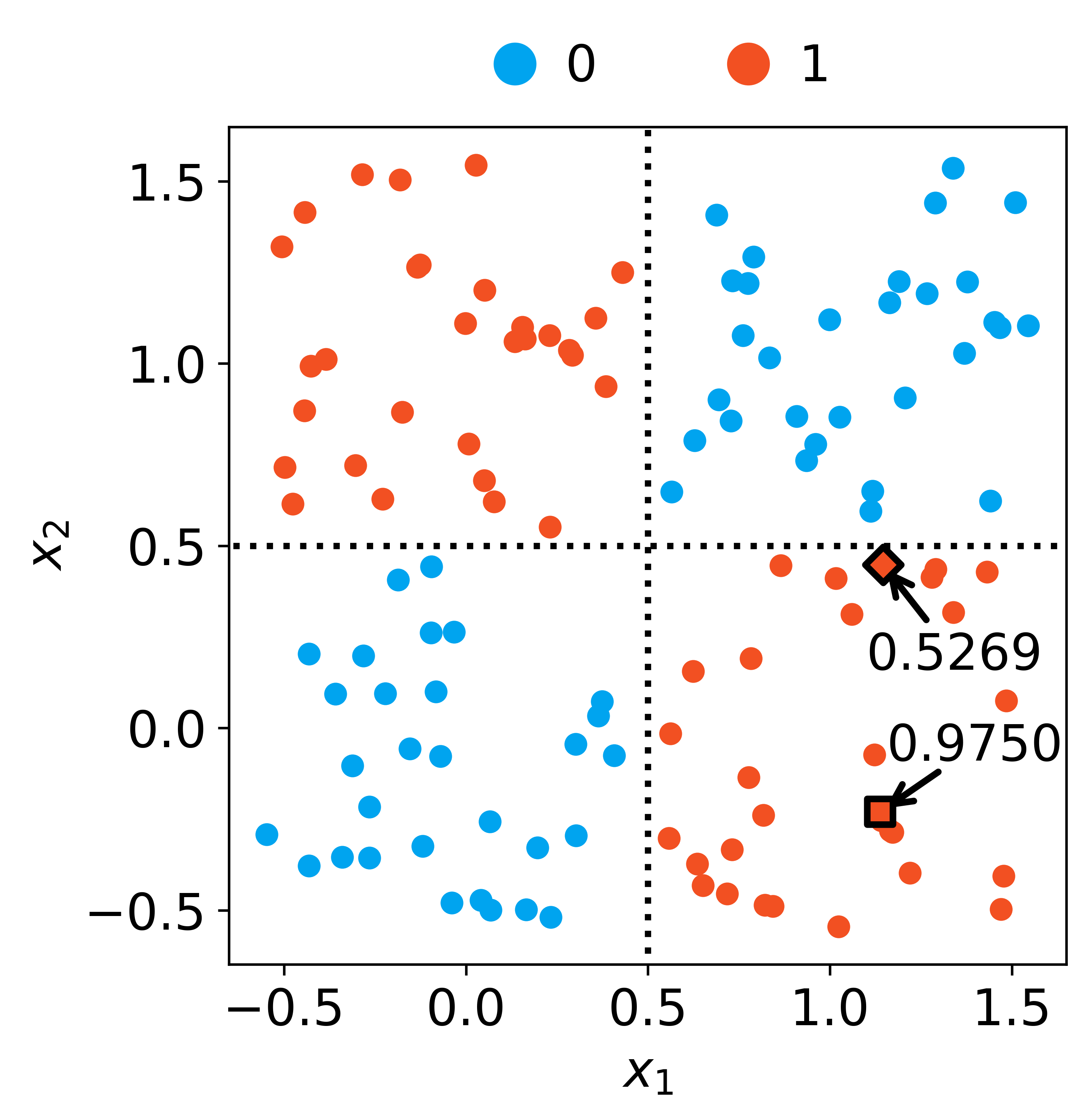
Figure 5(a) visualizes the noisy XOR test set of subsection 4.1. This is the same test set shown in figure 2(a), but with test points coloured according to their labels. Figure 5(b) shows the posterior predictive probability $p(y=c|(x_{1},x_{2}),D_{1:500})$ of true label $c\in\{0,1\}$ for each noisy XOR test point $((x_{1},x_{2}),y=c)$ given noisy XOR training set $D_{1:500}$ of subsection 4.1. The posterior probabilities $p(y=c|(x_{1},x_{2}),D_{1:500})$ of predicting true class $c$ are ordered within class $c$. Moreover, each $p(y=c|(x_{1},x_{2}),D_{1:500})$ is coloured as red or pale green depending on whether the resulting prediction is correct or not. One of the ten MH chain realizations for $\mbox{MLP}(2,2,1)$ parameter inference from noisy XOR data is used for approximating $p(y=c|(x_{1},x_{2}),D_{1:500})$ via (3.11) and for making predictions via (3.12).

Two points in the noisy XOR test set are marked in figure 5 using a square and a rhombus. These two points have the same true label $c=1$. Given posterior predictive probabilities $0.5269$ and $0.9750$ for the rhombus and square-shaped test points, the label $c=1$ is correctly predicted for both points. However, the rhombus-shaped point is closer to the decision boundary $x_{2}=0.5$ than the square-shaped point, so classifying the former entails higher uncertainty. As $0.5269<0.9750$, Bayesian marginalization quantifies the increased predictive uncertainty associated with the rhombus-shaped point despite using a non-converged MH chain realization.

Figure 6(a) shows a scatterplot of weight against tail length for the hawk test set of subsection 4.1. Blue, red and green test points belong to Cooper’s, red-tailed and sharp-shinned hawk classes. Figure 6(b) shows the posterior predictive probabilities $p(y=c|x,D_{1:596})$ for a subset of $100$ hawk test points, where $c\in\{\mbox{Cooper's},\mbox{red-tailed},\mbox{sharp-shinned}\}$ denotes the true label of test point $(x,y=c)$ and $D_{1:596}$ denotes the hawk training set of subsection 4.1. These posterior predictive probabilities are shown ordered within each class, and are coloured red or pale green depending on whether they yield correct or wrong predictions. One of the ten MH chain realizations for $\mbox{MLP}(6,2,2,3)$ parameter inference is used for approximating $p(y=c|x,D_{1:596})$ via (3.11) and for making predictions via (3.13).

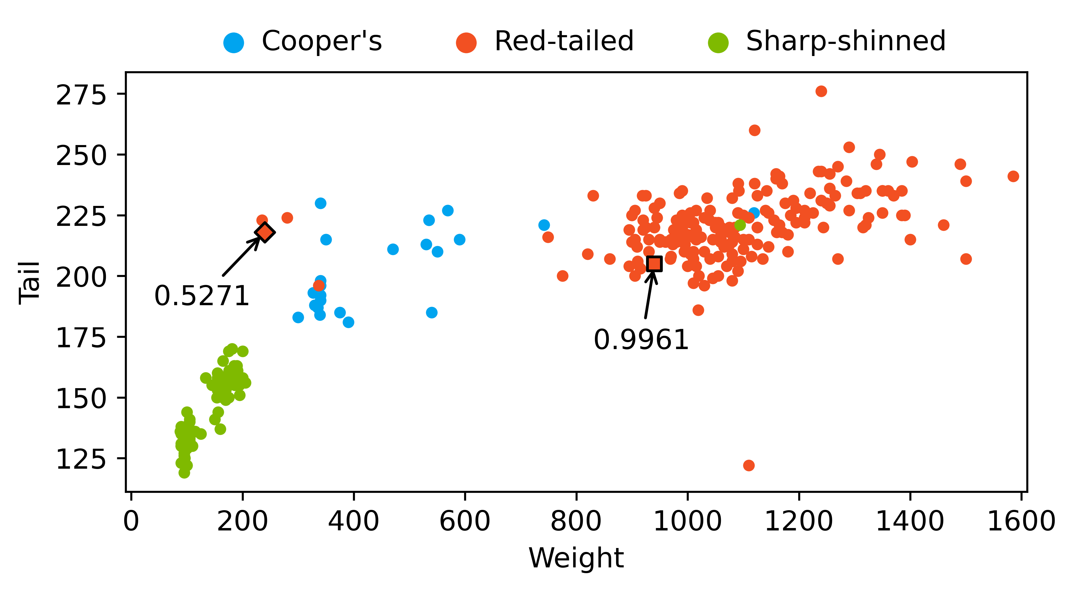
Two points in the hawk test set are marked in figure 6 using a square and a rhombus. Each of these two points represents weight and tail length measurements from a red-tailed hawk. The red-tailed hawk class is correctly predicted for both points. The squared-shaped observation belongs to the main cluster of red-tailed hawks in figure 6(a) and it is predicted with high posterior predictive probability ($0.9961$). On the other hand, the rhombus-shaped observation, which falls in the cluster of Cooper’s hawk, is correctly predicted with a lower posterior predictive probability ($0.5271$). Bayesian marginalization provides approximate posterior predictive probabilities that signify the level of uncertainty in predictions despite using a non-converged MH chain realization.

References

- Andrieu, de Freitas and Doucet (1999) [author] Andrieu, C.C., de Freitas, J. F. G.J. F. G. and Doucet, A.A. (1999). Sequential Bayesian estimation and model selection applied to neural networks.
- Andrieu, de Freitas and Doucet (2000) Andrieu, C., de Freitas, N. and Doucet, A. (2000). Reversible jump MCMC simulated annealing for neural networks. In Proceedings of the Sixteenth Conference on Uncertainty in Artificial Intelligence 11–18.
- Ashukha et al. (2020) Ashukha, A., Lyzhov, A., Molchanov, D. and Vetrov, D. (2020). Pitfalls of in-domain uncertainty estimation and ensembling in deep learning. In International Conference on Learning Representations.
- Badrinarayanan, Mishra and Cipolla (2015) [author] Badrinarayanan, VijayV., Mishra, BamdevB. and Cipolla, RobertoR. (2015). Symmetry-invariant optimization in deep networks. arXiv.
- (5) [author] Bennett, James EJ. E., Racine-Poon, AmyA. and Wakefield, Jon CJ. C. MCMC for nonlinear hierarchical models. 339–358.
- Bernardo (1979) [author] Bernardo, Jose M.J. M. (1979). Reference posterior distributions for Bayesian inference. Journal of the Royal Statistical Society. Series B (Methodological) 41 113–147.
- Blei, Kucukelbir and McAuliffe (2017) [author] Blei, David M.D. M., Kucukelbir, AlpA. and McAuliffe, Jon D.J. D. (2017). Variational inference: a review for statisticians. Journal of the American Statistical Association 112 859-877.
- Blier and Ollivier (2018) Blier, L. and Ollivier, Y. (2018). The description length of deep learning models. In Advances in Neural Information Processing Systems 31.
- Brea et al. (2019) [author] Brea, JohanniJ., Simsek, BerfinB., Illing, BerndB. and Gerstner, WulframW. (2019). Weight-space symmetry in deep networks gives rise to permutation saddles, connected by equal-loss valleys across the loss landscape. arXiv.
- Brooks and Gelman (1998) [author] Brooks, Stephen P.S. P. and Gelman, AndrewA. (1998). General methods for monitoring convergence of iterative simulations. Journal of Computational and Graphical Statistics 7 434–455.
- Cannon et al. (2019) Cannon, A., Cobb, G., Hartlaub, B., Legler, J., Lock, R., Moore, T., Rossman, A. and Witmer, J. (2019). Stat2Data: datasets for Stat2 R package version 2.0.0.
- Chen, Fox and Guestrin (2014) Chen, T., Fox, E. and Guestrin, C. (2014). Stochastic gradient Hamiltonian Monte Carlo. In Proceedings of the 31st International Conference on Machine Learning 32 1683–1691.
- Chen, Lu and Hecht-Nielsen (1993) [author] Chen, A. M.A. M., Lu, H.H. and Hecht-Nielsen, R.R. (1993). On the geometry of feedforward neural network error surfaces. Neural Computation 5 910–927.
- Chen et al. (2019) Chen, W. Y., Barp, A., Briol, F.-X., Gorham, J., Girolami, M., Mackey, L. and Oates, C. (2019). Stein point Markov chain Monte Carlo. In Proceedings of the 36th International Conference on Machine Learning 97 1011–1021.
- Chollet (2017) Chollet, F. (2017). Xception: deep learning with depthwise separable convolutions. In Proceedings of the IEEE conference on computer vision and pattern recognition 1251–1258.
- Chwialkowski, Strathmann and Gretton (2016) Chwialkowski, K., Strathmann, H. and Gretton, A. (2016). A kernel test of goodness of fit. In Proceedings of The 33rd International Conference on Machine Learning 48 2606–2615.
- Cowles and Carlin (1996) [author] Cowles, Mary KathrynM. K. and Carlin, Bradley P.B. P. (1996). Markov chain Monte Carlo convergence diagnostics: a comparative review. Journal of the American Statistical Association 91 883–904.
- Cybenko (1989) [author] Cybenko, GeorgeG. (1989). Approximation by superpositions of a sigmoidal function. Mathematics of control, signals and systems 2 303–314.
- Dai and Jones (2017) [author] Dai, NingN. and Jones, Galin L.G. L. (2017). Multivariate initial sequence estimators in Markov chain Monte Carlo. Journal of Multivariate Analysis 159 184–199.
- Daniels and Kass (1998) [author] Daniels, Michael J.M. J. and Kass, Robert E.R. E. (1998). A note on first-stage approximation in two-stage hierarchical models. Sankhyā: The Indian Journal of Statistics, Series B (1960-2002) 60 19–30.
- de Freitas (1999) [author] de Freitas, NandoN. (1999). Bayesian methods for neural networks, PhD thesis, University of Cambridge.
- de Freitas et al. (2001) [author] de Freitas, N.N., Andrieu, C.C., Højen-Sørensen, P.P., Niranjan, M.M. and Gee, A.A. (2001). Sequential Monte Carlo methods for neural networks In Sequential Monte Carlo Methods in Practice 359–379.
- De Sa, Chen and Wong (2018) De Sa, C., Chen, V. and Wong, W. (2018). Minibatch Gibbs sampling on large graphical models. In Proceedings of the 35th International Conference on Machine Learning 80 1165–1173.
- Dupuy and Bach (2017) [author] Dupuy, ChristopheC. and Bach, FrancisF. (2017). Online but accurate inference for latent variable models with local Gibbs sampling. Journal of Machine Learning Research 18 1-45.
- Ensign et al. (2017) Ensign, D., Neville, S., Paul, A. and Venkatasubramanian, S. (2017). The complexity of explaining neural networks through (group) invariants. In Proceedings of the 28th International Conference on Algorithmic Learning Theory 76 341–359.
- Esmaeili et al. (2019) Esmaeili, B., Wu, H., Jain, S., Bozkurt, A., Siddharth, N., Paige, B., Brooks, D. H., Dy, J. and van de Meent, J.-W. (2019). Structured disentangled representations. In Proceedings of the 22nd International Conference on Artificial Intelligence and Statistics 89 2525–2534.
- Freeman, Roese-Koerner and Kummert (2018) Freeman, I., Roese-Koerner, L. and Kummert, A. (2018). Effnet: An efficient structure for convolutional neural networks. In 25th IEEE International Conference on Image Processing 6–10.
- Friel and Pettitt (2008) [author] Friel, N.N. and Pettitt, A. N.A. N. (2008). Marginal likelihood estimation via power posteriors. Journal of the Royal Statistical Society: Series B (Statistical Methodology) 70 589–607.
- Gelman and Rubin (1992) [author] Gelman, AndrewA. and Rubin, Donald B.D. B. (1992). Inference from iterative simulation using multiple sequences. Statistical Science 7 457–472.
- Gelman et al. (2004) [author] Gelman, AndrewA., Carlin, John BJ. B., Stern, Hal SH. S. and Rubin, Donald BD. B. (2004). Bayesian data analysis, 2nd ed. Chapman and Hall/CRC.
- (31) [author] Gilks, Walter RW. R. and Roberts, Gareth OG. O. Strategies for improving MCMC. 89–114.
- Giordano, Broderick and Jordan (2015) [author] Giordano, Ryan JR. J., Broderick, TamaraT. and Jordan, Michael IM. I. (2015). Linear response methods for accurate covariance estimates from mean field variational Bayes. In Advances in Neural Information Processing Systems 28 1441–1449.
- Gong and Flegal (2016) [author] Gong, LeiL. and Flegal, James M.J. M. (2016). A practical sequential stopping rule for high-dimensional Markov chain Monte Carlo. Journal of Computational and Graphical Statistics 25 684–700.
- Gong, Li and Hernández-Lobato (2019) Gong, W., Li, Y. and Hernández-Lobato, J. M. (2019). Meta-learning For stochastic gradient MCMC. In International Conference on Learning Representations.
- Goodfellow, Bengio and Courville (2016) [author] Goodfellow, IanI., Bengio, YoshuaY. and Courville, AaronA. (2016). Deep learning. MIT press.
- Graf and Luschgy (2007) [author] Graf, SiegfriedS. and Luschgy, HaraldH. (2007). Foundations of quantization for probability distributions. Springer.
- Gretton et al. (2012) [author] Gretton, ArthurA., Borgwardt, Karsten MK. M., Rasch, Malte JM. J., Schölkopf, BernhardB. and Smola, AlexanderA. (2012). A kernel two-sample test. Journal of Machine Learning Research 13 723–773.
- Gu, Ghahramani and Turner (2015) [author] Gu, Shixiang (Shane)S. S., Ghahramani, ZoubinZ. and Turner, Richard ER. E. (2015). Neural adaptive sequential Monte Carlo. In Advances in Neural Information Processing Systems 28 2629–2637.
- Hastie, Tibshirani and Friedman (2016) [author] Hastie, TrevorT., Tibshirani, RobertR. and Friedman, JeromeJ. (2016). The elements of statistical learning: data mining, inference and prediction, 2nd ed. Springer.
- Hastings (1970) [author] Hastings, W. K.W. K. (1970). Monte Carlo sampling methods using Markov chains and their applications. Biometrika 57 97–109.
- Hecht-Nielsen (1990) [author] Hecht-Nielsen, RobertR. (1990). On the algebraic structure of feedforward network weight spaces. In Advanced Neural Computers 129–135.
- Hornik (1991) [author] Hornik, KurtK. (1991). Approximation capabilities of multilayer feedforward networks. Neural Networks 4 251–257.
- Horst, Hill and Gorman (2020) Horst, A. M., Hill, A. P. and Gorman, K. B. (2020). palmerpenguins: Palmer Archipelago (Antarctica) penguin data R package version 0.1.0.
- Howard et al. (2017) [author] Howard, Andrew GA. G., Zhu, MenglongM., Chen, BoB., Kalenichenko, DmitryD., Wang, WeijunW., Weyand, TobiasT., Andreetto, MarcoM. and Adam, HartwigH. (2017). Mobilenets: efficient convolutional neural networks for mobile vision applications. arXiv.
- Hu, Zagoruyko and Komodakis (2019) [author] Hu, Shell XuS. X., Zagoruyko, SergeyS. and Komodakis, NikosN. (2019). Exploring weight symmetry in deep neural networks. Computer Vision and Image Understanding 187 102786.
- Huang et al. (2019) Huang, C.-W., Sankaran, K., Dhekane, E., Lacoste, A. and Courville, A. (2019). Hierarchical importance weighted autoencoders. In Proceedings of the 36th International Conference on Machine Learning 97 2869–2878.
- Iandola et al. (2016) [author] Iandola, Forrest NF. N., Han, SongS., Moskewicz, Matthew WM. W., Ashraf, KhalidK., Dally, William JW. J. and Keutzer, KurtK. (2016). SqueezeNet: AlexNet-level accuracy with 50x fewer parameters and ¡0.5MB model size. arXiv.
- Izmailov et al. (2020) Izmailov, P., Maddox, W. J., Kirichenko, P., Garipov, T., Vetrov, D. and Wilson, A. G. (2020). Subspace inference for Bayesian deep learning. In Proceedings of The 35th Uncertainty in Artificial Intelligence Conference 115 1169–1179.
- Jarrett et al. (2009) Jarrett, K., Kavukcuoglu, K., Ranzato, M. and LeCun, Y. (2009). What is the best multi-stage architecture for object recognition? In IEEE 12th International Conference on Computer Vision 2146-2153.
- Jaynes (1968) [author] Jaynes, E. T.E. T. (1968). Prior probabilities. IEEE Transactions on Systems Science and Cybernetics 4 227–241.
- Jeffreys (1962) [author] Jeffreys, HaroldH. (1962). The theory of probability, 3rd ed. OUP Oxford.
- Johndrow, Pillai and Smith (2020) [author] Johndrow, James E.J. E., Pillai, Natesh S.N. S. and Smith, AaronA. (2020). No free lunch for approximate MCMC. arXiv.
- Kass et al. (1998) [author] Kass, Robert E.R. E., Carlin, Bradley P.B. P., Gelman, AndrewA. and Neal, Radford M.R. M. (1998). Markov chain Monte Carlo in practice: a roundtable discussion. The American Statistician 52 93–100.
- Krizhevsky, Sutskever and Hinton (2012) [author] Krizhevsky, AlexA., Sutskever, IlyaI. and Hinton, Geoffrey EG. E. (2012). ImageNet classification with deep convolutional neural networks. In Advances in Neural Information Processing Systems 25 1097–1105.
- Lee (2000) [author] Lee, H. K. H.H. K. H. (2000). Consistency of posterior distributions for neural networks. Neural Networks 13 629–642.
- Lee (2003) [author] Lee, Herbert K. H.H. K. H. (2003). A noninformative prior for neural networks. Machine Learning 50 197–212.
- Lee (2004) [author] Lee, Herbert KHH. K. (2004). Priors for neural networks. In Classification, Clustering, and Data Mining Applications (DavidD. Banks, Frederick R.F. R. McMorris, PhippsP. Arabie and WolfgangW. Gaul, eds.) 141–150.
- Lee (2005) Lee, H. K. (2005). Neural networks and default priors. In Proceedings of the American Statistical Association, Section on Bayesian Statistical Science.
- Lee (2007) [author] Lee, Herbert KHH. K. (2007). Default priors for neural network classification. Journal of Classification 24 53–70.
- Lu et al. (2017) [author] Lu, ZhouZ., Pu, HongmingH., Wang, FeichengF., Hu, ZhiqiangZ. and Wang, LiweiL. (2017). The expressive power of neural networks: a view from the width. In Advances in Neural Information Processing Systems 30 6231–6239.
- Ma, Foti and Fox (2017) Ma, Y.-A., Foti, N. J. and Fox, E. B. (2017). Stochastic gradient MCMC methods for hidden Markov models. In Proceedings of the 34th International Conference on Machine Learning 70 2265–2274.
- MacKay (1995) [author] MacKay, David JCD. J. (1995). Developments in probabilistic modelling with neural networks—ensemble learning. In Neural Networks: Artificial Intelligence and Industrial Applications 191–198.
- Maddison et al. (2015) Maddison, C. J., Huang, A., Sutskever, I. and Silver, D. (2015). Move evaluation in Go using deep convolutional neural networks. In International Conference on Learning Representations.
- Mandt, Hoffman and Blei (2017) [author] Mandt, StephanS., Hoffman, Matthew D.M. D. and Blei, David M.D. M. (2017). Stochastic gradient descent as approximate Bayesian inference. Journal of Machine Learning Research 18 1–35.
- Metropolis et al. (1953) [author] Metropolis, NicholasN., Rosenbluth, Arianna WA. W., Rosenbluth, Marshall NM. N., Teller, Augusta HA. H. and Teller, EdwardE. (1953). Equation of state calculations by fast computing machines. The journal of Chemical Physics 21 1087–1092.
- Minsky and Papert (1988) [author] Minsky, Marvin LM. L. and Papert, Seymour AS. A. (1988). Perceptrons: expanded edition. MIT press.
- Moore (2016) Moore, D. A. (2016). Symmetrized variational inference. In NIPS Workshop on Advances in Approximate Bayesian Inference.
- Nair and Hinton (2009) [author] Nair, VinodV. and Hinton, Geoffrey EG. E. (2009). 3D object recognition with deep belief nets. In Advances in Neural Information Processing Systems 22 1339–1347.
- Nalisnick (2018) [author] Nalisnick, Eric ThomasE. T. (2018). On priors for Bayesian neural networks, PhD thesis, UC Irvine.
- Neal (2011) [author] Neal, R. M.R. M. (2011). MCMC Using Hamiltonian dynamics In Handbook of Markov Chain Monte Carlo 5. CRC Press.
- Nemeth and Sherlock (2018) [author] Nemeth, ChristopherC. and Sherlock, ChrisC. (2018). Merging MCMC subposteriors through Gaussian-process approximations. Bayesian Analysis 13 507–530.
- Nwankpa et al. (2018) [author] Nwankpa, ChigozieC., Ijomah, WinifredW., Gachagan, AnthonyA. and Marshall, StephenS. (2018). Activation functions: comparison of trends in practice and research for deep learning. arXiv.
- Ong, Nott and Smith (2018) [author] Ong, Victor M. H.V. M. H., Nott, David J.D. J. and Smith, Michael S.M. S. (2018). Gaussian variational approximation with a factor covariance structure. Journal of Computational and Graphical Statistics 27 465–478.
- Pearce et al. (2019) Pearce, T., Zaki, M., Brintrup, A. and Neely, A. (2019). Expressive priors in Bayesian neural networks: kernel combinations and periodic functions. In Proceedings of the 35th Conference on Uncertainty in Artificial Intelligence.
- Polson and Sokolov (2017) [author] Polson, Nicholas G.N. G. and Sokolov, VadimV. (2017). Deep learning: a Bayesian perspective. Bayesian Analysis 12 1275–1304.
- Pourzanjani, Jiang and Petzold (2017) Pourzanjani, A. A., Jiang, R. M. and Petzold, L. R. (2017). Improving the identifiability of neural networks for Bayesian inference. In NIPS Workshop on Bayesian Deep Learning.
- Quiroz et al. (2019) [author] Quiroz, MatiasM., Kohn, RobertR., Villani, MattiasM. and Tran, Minh-NgocM.-N. (2019). Speeding Up MCMC by efficient data subsampling. Journal of the American Statistical Association 114 831–843.
- Ranganath, Tran and Blei (2016) Ranganath, R., Tran, D. and Blei, D. (2016). Hierarchical variational models. In Proceedings of The 33rd International Conference on Machine Learning 48 324–333.
- Robert et al. (2018) [author] Robert, Christian P.C. P., Elvira, VíctorV., Tawn, NickN. and Wu, ChangyeC. (2018). Accelerating MCMC algorithms. Wiley Interdisciplinary Reviews: Computational Statistics 10 e1435.
- Rosenblatt (1958) [author] Rosenblatt, FrankF. (1958). The perceptron: a probabilistic model for information storage and organization in the brain. Psychological review 65 386.
- Rudolf and Schweizer (2018) [author] Rudolf, DanielD. and Schweizer, NikolausN. (2018). Perturbation theory for Markov chains via Wasserstein distance. Bernoulli 24 2610–2639.
- Sargent, Hodges and Carlin (2000) [author] Sargent, Daniel J.D. J., Hodges, James S.J. S. and Carlin, Bradley P.B. P. (2000). Structured Markov chain Monte Carlo. Journal of Computational and Graphical Statistics 9 217–234.
- Seita et al. (2018) Seita, D., Pan, X., Chen, H. and Canny, J. (2018). An efficient minibatch acceptance test for Metropolis-Hastings. In Proceedings of the Twenty-Seventh International Joint Conference on Artificial Intelligence 5359–5363.
- Sen, Papamarkou and Dunson (2020) [author] Sen, DeborsheeD., Papamarkou, TheodoreT. and Dunson, DavidD. (2020). Bayesian neural networks and dimensionality reduction. arXiv.
- Simpson et al. (2017) [author] Simpson, DanielD., Rue, HåvardH., Riebler, AndreaA., Martins, Thiago G.T. G. and Sørbye, Sigrunn H.S. H. (2017). Penalising model component complexity: a principled, practical approach to constructing priors. Statistical Science 32 1–28.
- Smith et al. (1988) Smith, J. W., Everhart, J., Dickson, W., Knowler, W. and Johannes, R. (1988). Using the ADAP learning algorithm to forecast the onset of diabetes mellitus. In Proceedings of the Annual Symposium on Computer Application in Medical Care 261.
- Stephens (2000) [author] Stephens, M.M. (2000). Dealing with label switching in mixture models. Journal of the Royal Statistical Society: Series B (Statistical Methodology) 62 795–809.
- Titsias and Ruiz (2019) Titsias, M. K. and Ruiz, F. (2019). Unbiased implicit variational inference. In Proceedings of Machine Learning Research 89 167–176.
- Titterington (2004) [author] Titterington, D. M.D. M. (2004). Bayesian methods for neural networks and related models. Statistical Science 19 128–139.
- Truong, Nguyen and Tran (2018) Truong, T.-D., Nguyen, V.-T. and Tran, M.-T. (2018). Lightweight Deep Convolutional Network for Tiny Object Recognition. In Proceedings of the 7th International Conference on Pattern Recognition Applications and Methods 675–682.
- Vats and Flegal (2018) [author] Vats, DootikaD. and Flegal, James MJ. M. (2018). Lugsail lag windows and their application to MCMC. arXiv.
- Vats, Flegal and Jones (2019) [author] Vats, DootikaD., Flegal, James MJ. M. and Jones, Galin LG. L. (2019). Multivariate output analysis for Markov chain Monte Carlo. Biometrika 106 321–337.
- Vats and Knudson (2018) [author] Vats, DootikaD. and Knudson, ChristinaC. (2018). Revisiting the Gelman-Rubin diagnostic. arXiv.
- Vehtari et al. (2019) [author] Vehtari, AkiA., Gelman, AndrewA., Simpson, DanielD., Carpenter, BobB. and Burkner, Paul-ChristianP.-C. (2019). Rank-normalization, folding, and localization: an improved R for assessing convergence of MCMC. arXiv.
- Vladimirova et al. (2019) Vladimirova, M., Verbeek, J., Mesejo, P. and Arbel, J. (2019). Understanding priors in Bayesian neural networks at the unit level. In Proceedings of the 36th International Conference on Machine Learning 97 6458–6467.
- Welling and Teh (2011) Welling, M. and Teh, Y. W. (2011). Bayesian learning via stochastic gradient Langevin dynamics. In Proceedings of the 28th International Conference on International Conference on Machine Learning 681–688.
- Williams (1995) [author] Williams, Peter M.P. M. (1995). Bayesian regularization and pruning using a Laplace prior. Neural Computation 7 117–143.
- Williams (2000) [author] Williams, Christopher K. I.C. K. I. (2000). An MCMC approach to hierarchical mixture modelling. In Advances in Neural Information Processing Systems 12 680–686.
- Wilson and Izmailov (2020) [author] Wilson, Andrew GordonA. G. and Izmailov, PavelP. (2020). Bayesian deep learning and a probabilistic perspective of generalization. arXiv.
- Zhang et al. (2018a) Zhang, G., Sun, S., Duvenaud, D. and Grosse, R. (2018a). Noisy natural gradient as variational inference. In Proceedings of the 35th International Conference on Machine Learning 80 5852–5861.
- Zhang et al. (2018b) Zhang, X., Zhou, X., Lin, M. and Sun, J. (2018b). Shufflenet: An extremely efficient convolutional neural network for mobile devices. In Proceedings of the IEEE Conference on Computer Vision and Pattern Recognition 6848–6856.