1
Shapley Homology: Topological Analysis of Sample Influence for Neural Networks
Kaixuan Zhang1,
Qinglong Wang2,
Xue Liu
C. Lee Giles1
1Pennsylvania State University.
2McGill University.
Keywords: Topological data analysis, homology, Shapley value, sample influence, deep learning.
Abstract
Data samples collected for training machine learning models are typically assumed to be independent and identically distributed (iid). Recent research has demonstrated that this assumption can be problematic as it simplifies the manifold of structured data. This has motivated different research areas such as data poisoning, model improvement, and explanation of machine learning models. In this work, we study the influence of a sample on determining the intrinsic topological features of its underlying manifold. We propose the Shapley Homology framework, which provides a quantitative metric for the influence of a sample of the homology of a simplicial complex. By interpreting the influence as a probability measure, we further define an entropy which reflects the complexity of the data manifold. Our empirical studies show that when using the -dimensional homology, on neighboring graphs, samples with higher influence scores have more impact on the accuracy of neural networks for determining the graph connectivity and on several regular grammars whose higher entropy values imply more difficulty in being learned.
1 Introduction
In much machine learning research, it is common practice to assume that the training samples are independent and identically distributed (iid). As such, samples are implicitly regarded as having equal influence on determining the performance of a machine learning model. Recently, limitations of this assumption have been explored. For example, a recent study (Koh & Liang (2017)) showed that certain training samples can have significant influences over a model’s decisions for certain testing samples. This effect has motivated research on model interpretation (Gunning (2017); Koh & Liang (2017); Yeh et al. (2018)), model & algorithm improvement (Lee & Yoo (2019); T. Wang et al. (2018); Ren et al. (2018)), and poisoning attacks (Y. Wang & Chaudhuri (2018); Koh & Liang (2017); X. Chen et al. (2017)).
Many of the aforementioned methods study the sample influence problem by using neural networks. Specifically, it is common to adopt a neural network (either a target model or a surrogate) to identify samples that are deemed as more influential (Koh & Liang (2017); T. Wang et al. (2018)). However, as shown by X. Chen et al. (2017) in a poisoning attack scenario, a limited number of poisoning samples can be effective in applying a backdoor attack in a model-agnostic manner. This motivates work that studies the intrinsic properties of data so that one can develop countermeasures to methods that defeat learning models. Specifically, by representing the underlying space of data as a topological space, we study the sample influence problem from a topological perspective. The belief that topological features of the data space better represent its intrinsic properties has attracted recent research on establishing relationships between machine learning and topological data analysis (TDA) (Chazal & Michel (2017); Hofer et al. (2017); Carlsson & Gabrielsson (2018)).
In this work, we consider TDA as a complementary approach to other approaches that study sample influence. We propose a framework for decomposing the topological features of a complex (built with data points and certain homology group) to individual points. We interpret the decomposed value for each point as representing its influence on affecting its topological features. We then calculate that influence as Shapley values (Narahari (2012)). Recent research (J. Chen et al. (2018); Lundberg & Lee (2017); Datta et al. (2016)) proposed similar approaches to quantify feature influence. By interpreting the influence as a probability measure defined on a data space, we also calculate the entropy which describes the complexity of this space. Under our framework and with proper configurations of the topological space, we devise an algorithm for calculating the influence of data samples and entropy for any data set.
We perform both analytical and empirical studies on several sets of data samples from two families of structured data – graphs and strings. Specifically, we generate random graphs using the Erdos-Renyi model and binary strings with regular grammars. In both cases, we use neural networks as verification tools for our analysis of sample influence. Explicitly, we employ a feed-forward network trained to determine the connectivity of the generated graphs, and a recurrent network trained to recognize the generated strings. Our results show that samples identified by our method as having more significant influence indeed have more impact on the connectivity of their underlying graphs, and that grammars with higher complexity have more difficulty in being learned.
2 Related Work
2.1 Sample Influence
There have been several research efforts to explore and exploit influential samples for various purposes. As an example, by analyzing how the performance of a model at the testing phase affects a small number of training samples motivated research in poisoning attacks (Y. Wang & Chaudhuri (2018); Koh & Liang (2017); X. Chen et al. (2017)). In this case, a limited number of corrupted training examples are injected to degrade a target model’s performance. An alternative thread of research exploits this effect to improve the generalization accuracy of learning models and the efficiency of learning algorithms. Specifically, influential samples can be identified via learning then used for enhancing models’ performance on imbalance and corrupted data (Ren et al. (2018); Lee & Yoo (2019)). They can also be synthesized to represent a much larger set of samples hence accelerating the learning process (T. Wang et al. (2018)). Besides, influential samples can bring explainability to deep learning models by identifying representative samples or prototypes used in decision making (Yeh et al. (2018); Anirudh et al. (2017)).
2.2 Topological Data Analysis
The most widely-used tool from TDA is persistent homology (Chazal & Michel (2017)), which an algebraic method for measuring topological features of shapes and functions. Persistent homology provides a multi-scale analysis of underlying geometric structures represented by persistence barcode or diagram. Most of the previous research using persistence homology focused on the classification task of some certain manifold constructed by data points (Carlsson et al. (2008); Li et al. (2014); Turner et al. (2014)), and mapping the topological signatures to machine learning representations (Carlsson & Gabrielsson (2018); Bubenik (2015)). Unlike previous work, our proposed framework Shapley Homology emphasizes the individual influence of vertex on the topological space and generalizing the global features of the data set.
3 Shapley Homology
Here, we first introduce the relevant concepts that are necessary for our Shapley Homology framework. We then provide the definitions of sample influence and entropy.
3.1 ech Complex and Homology Group
ech Complex
In topological analysis, the study of a set of data points is typically based on simplicial complexes, which provide more abstract generalizations of neighboring graphs that describe the structural relationships between data points. Here, we are particularly interested in the ech complex, which is an abstract simplicial complex. More formally, the definition of the ech complex is as follows.
Definition 1 (ech complex).
The ech complex is the intersection complex or nerve of the set of balls of radius centered at points in .
In particular, given a finite point cloud in a metric space and a radius , the ech complex can be constructed by first taking the points in as a vertex set of . Then for each set , let if the set of -balls centered at points of has a nonempty intersection. Note, that the ech complex has a property showing that the simplicial complex constructed with a smaller is a subcomplex of that with a larger .
Homology
The topological features of data space are typically formalized and studied through Homology, which is a classical concept in algebraic topology (Chazal & Michel (2017)). In the following, we briefly introduce homology to the extent that is necessary for understanding its role in our framework.
Definition 2 (Homology Group).
A chain complex is a sequence of abelian groups or modules connected by homomorphisms , such that the composition of any two consecutive maps is the zero map. The -th homology group is the group of cycles modulo boundaries in degree , that is,
| (1) |
where and im denotes the kernel and image of homomorphism, respectively.
Generally speaking, the -th homology is a quotient group that indicates the -dimensional independent features of the space . Particularly, when , we have the following proposition (Hatcher (2005)):
Proposition 1.
For any space , is a direct sum of abelian groups, one for each path-component of .
Specially, when a complex takes the form of a neighboring graph, then the -homology denote the subgraphs that are connected in this graph. As for the -homology , it represents the number of genus in the given manifold.
3.2 Sample Influence and Entropy
Given a point cloud represented by a ech complex, we study the influence of each data point on the topological features of this complex. This influence of a data point can be further interpreted as the probability that a unit change of the topological feature is caused by this point. More formally, denote a data set containing samples by , we have the following definition of sample influence.
Definition 3 (Sample Influence).
The influence of any sample (or subset) is a probability measure .
We can then define a canonical entropy of the set as follows.
Definition 4 (Entropy).
Given a probability measure , the entropy of a dataset is defined as .

3.3 The Framework of Shapley Homology
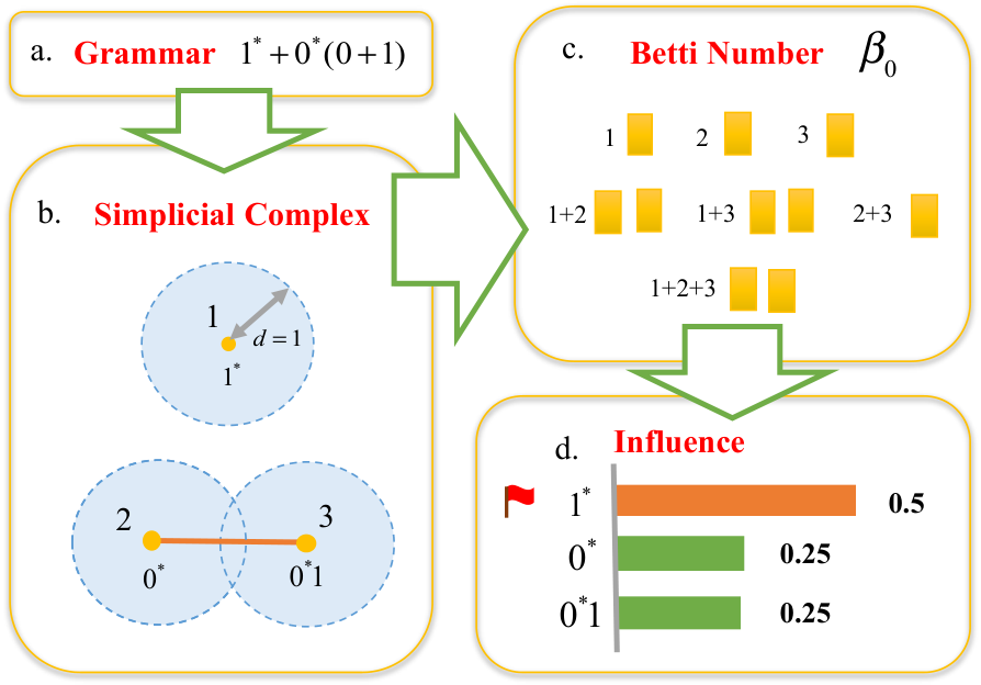
Here we propose a framework (depicted in Figure 1) of Shapley Homology in order to study sample influence. Specifically, in Figure 1, we provide an example for investigating a specific topological feature – the Betti number (Rote & Vegter (2006)) –of a topological space. As will become clear from the following, the Betti number can be used to quantify the homology group of topological space according to its connectivity.
Definition 5 (Betti Number).
Given a non-negative integer , the -th Betti number of the space is defined as the rank of the abelian group , that is,
| (2) |
Following the definition, as there are no special structures (such as real projective space in the complex), the Betti number indicates the number of direct sum of abelian groups of the -th homology group11 1 Generally speaking, the Betti number of a finitely generated abelian group is the (uniquely determined) number such that where are finite cyclic groups. But for real projective space , the homology group with coefficients in integers is Hence for odd , the number of abelian groups in is but actually the Betti number . This is not a concern for ech complex.. In other words, the -th Betti number refers to the number of -dimensional holes on a topological surface.
While the Betti number only indicates an overall feature of a complex, we need to further distribute this number to each vertex of this complex as its influence score. Recent research (J. Chen et al. (2018)) on interpreting neural networks has introduced Shapley value from cooperative game theory to decompose a classification score of a neural network made for a specific sample to individual features as their importance or contribution to rendering this classification result. Inspired by this line of work, we also employ the Shapley value as the influence score for each vertex. However, it should be noted that for a fixed , the Betti number does not satisfy the monotonicity property of Shapley values. That is, the Betti number of is not necessarily larger than that of when is a subcomplex of . As a result, we cannot adopt the formulation for calculating Shapley values directly. Here we use the following variant formulation for calculating Shapley values for a ech complex:
| (3) |
It is important to note that in our formulation (3), we use the absolute value to resolve the monotonicity issue. When the Betti number does satisfy the monotonicity property, then our calculation of Shapley values is the same as the canonical form.
It is clear that our formulation (3) satisfies the symmetry axiom, whereas, it does not satisfy other Shapley axioms, including the linearity and carrier axioms (Narahari (2012)). Nonetheless, our formulation still measures the marginal utility of a vertex. Besides, as we mainly focus on measuring the topological feature, both the decrease and increase in Betti number of a vertex are crucial for determining the influence. Furthermore, since our entropy is symmetry-invariant, its value will remain the same under the group action on the vertices (Conrad (2008)).
Above discussion indicates that the influence of a data sample can be regarded as a function of the radius , the Betti number , the size of the data set containing this sample, and the topological space constructed upon the chosen metric. Unlike persistence homology (Edelsbrunner & Harer (2008)), which studies the topological features of data space at varying “resolution” , our analysis takes a more static view of the topological features of a complex built with a fixed . As such, our analysis can be viewed as taking a slice from the filtration of used for persistence homology. In the following section, we propose an algorithm for calculating the influence scores of data points in a ech complex constructed with certain specified and .
4 Algorithm Design and Case Study
With Proposition 1 and Definition 5 and when the Betti number is regarded as a quantitative indicator, it equals the number of connected components in a complex. In this case, the task of calculating of a ech complex is equivalent to calculating the number of connected components of a graph. This enables us to compute the Laplacian matrix 22 2 The Laplacian matrix is defined to be where and denote the degree matrix and adjacency matrix respectively. of a graph then apply the following proposition (Marsden (2013)).
Proposition 2.
A graph has connected components if and only if the algebraic multiplicity of in the Laplacian is .
With the above proposition, we can see that the Betti number is equal to the number of zeros in the spectrum of the corresponding Laplacian matrix . As such, we propose the Algorithm 1 to calculate the influence score and the entropy under the setting of and as some constant. A more detailed discussion of the choice of and is provided in Section 5. In the meantime, it is important to note that this Algorithm 1 always produces a probability measure.
Here we provide a simple time complexity analysis for our algorithm and propose several possible solutions to accelerate the algorithm in our future work. Our algorithm can be decomposed into three parts: (1) complex construction; (2) calculation of graph spectrum; (3) assignment of the Shapley value. In the first step, since we need to calculate pairwise distance and form the adjacent matrix, it is clear that the complexity for this step is . In the second step, we need to compute the spectrum of all subcomplexes. As such, in total, the complexity is , where the complexity of each Laplacian decomposition is . As for the third step, we sum all the marginal utility for one sample, which results in the complexity of . Therefore, the complexity of computing the influence scores for all samples is . Based on the above analysis, we obtain the overall complexity of our algorithm as . Clearly, the second step and the third step contribute most to the total complexity. Specifically, in order to alleviate the computational burden caused by the second step, we will consider in our future work of various approaches (e.g., (Cohen-Steiner et al. (2018))) to approximate the spectrum of a graph. As for the third step, several existing approximation algorithms, e.g., C-Shapley and L-Shapley (J. Chen et al. (2018)), could be considered for approximating the Shapley value using local topological properties.
In the following, we provide a set of case studies on several different graphs with representative topological structures. In particular, we study four types of graphs representing the space of binary strings generated by four regular grammars. We select these grammars due to their simplicity for demonstration. A brief introduction of the selected grammars 33 3 Grammar 1, 2 and 4 are selected from the set of Tomita grammars (Tomita (1982)), of which their indices in the Tomita grammars are 1, 5 and 3, respectively. is provided in Table 1. Since we deal with binary string, we specify the distance metric used in these studies as the edit distance (De la Higuera (2010)) and set the radius . Also, we set the length of generated strings to fixed values as specified in Table 1.
Furthermore, we generalize our proposed framework to another six special sets of graphs and provide the analytical results of their vertices’ influence and the entropy values. These graphs are selected as they represent a set of simple complexes that can be used for building up more complicated topological structures.
| Description | Entropy | ||||||
|---|---|---|---|---|---|---|---|
| 1 | 0.00 | ||||||
| 2 | even number of 0s and even number of 1s. | ||||||
| 3 | |||||||
| 4 |
|
|
4.1 A Case Study on Regular Grammars
Simple Examples
Here we calculate and analyze the first three grammars shown in Table 1 as they have simple yet different topological features. As we can see from Table 1, for the first grammar, given a fixed , there exists only one string defined by this grammar. As a result, the influence of this sample is , and the entropy . For the second grammar, it is clear to see that any pair of valid strings have an edit distance larger than 1. In this case, the complex formed with the radius consists of disjoint points. Assuming that the there exist valid strings defined by this grammar with the length of , then all strings have the same influence and the entropy . For the third grammar, when the length of its associated strings is larger than 3, then the set of these strings can be expressed as , denoted as for notation simplicity. We depict the complex for the case when in Figure 2. According to Proposition 2, we then have the following Betti number of each subcomplex.
where () denotes the subgraph of formed by the vertex set . According to (3) and Algorithm 1, we have , and finally the entropy is .
A Complicated Example
The fourth grammar shown in Table 1 is more complicated than the three grammars mentioned above. In particular, let , or , then we illustrate the results in Figure 3, and the entropy is when and when . Besides the analytical results presented here, we further demonstrate the difference between this grammar and the first two grammars in a set of empirical studies in Section 6.2.
| Example | Shapley Value | Influence Score | ||||
|---|---|---|---|---|---|---|
|
|
|||||
| Cycles |
|
|||||
| Wheel Graph | Periphery: | Periphery: | ||||
| Center: | Center: | |||||
| Star | Periphery: | Periphery: | ||||
| Center: | Center: | |||||
| Path Graph | Ends: | Ends: | ||||
| Middle: | Middle: | |||||
| Complete Bipartite Graph | side: | side: | ||||
| side: | side: |
4.2 A Case Study on Special Graphs
In this part, we apply our framework to six special families of graphs, which are shown with examples in Table 2. Due to space constraint, here we omit the detailed calculation of the influence scores and entropy values for these graphs. With the analytical results shown in Table 2, it is easy to derive the following two corollaries:
Corollary 1.
for .
Corollary 2.
Suppose that is constant, then the value of decreases as increases.
5 Extended Discussion of Shapley Homology
As previously introduced in Section 3.3, our proposed influence score can be viewed as a function of the parameter and . Here we extend our study from the previous case of to cover other cases when , and show that adopting the -dimensional homology offers the merits of having more meaningful and practical implication. Also, we discuss the effect of selecting different radii on the topological features we study. More importantly, we show that our framework provides a more general view of sample influence and can be further adapted to capture the dynamical features of a topological space.
5.1 Discussion of the Choice of
We first consider the case when , since the homology group becomes less informative as increases. In this case, the Betti number represents the number of genus in a given manifold. Take the third grammar introduced in Section 4.1 as an example. It is clear to see that when using the -dimensional homology, all subcomplex has equal to 0. This is precisely the case when our algorithm cannot generate a probability measure. In a more general case, it is easy to show by the homology theory (Schapira (2001)) that once all subcomplex gets Betti number for some , then for any other -dimensional homology with , our framework cannot produce a probability measure. Furthermore, it is important to note that when adopting -dimensional homology with larger than 2, the corresponding Betti number only has rather abstract interpretation.
Another difficulty of adopting homology with higher dimension is due to the practical concern. More specifically, since it is challenging to calculate the homology when is large, one may need to apply tools such as Euler characteristic or Mayer-Vietoris Sequences (Hatcher (2005)), which is out the scope of this paper.
5.2 Discussion on the Choice of
The radius plays a critical role in building a manifold. For example, when is sufficiently small, the resulting complex contains only discrete data points with equal influence in our framework. When is sufficiently large, on the other hand, the complex is contractible, which indicates that there is no difference between the influence of data points contained in this complex. Both aforementioned extreme cases produce equal importance to the data points in a data set, and correspond to the i.i.d. assumption of sample distribution that is commonly taken in nowadays machine learning practice. In this sense, our framework provides a general abstraction of sample influence.
In practice, selecting a proper can be very difficult. This explains the usage of persistence homology (Edelsbrunner & Harer (2008)), which studies the evolution of topological features of a space as dynamically changes. This motivates future research of extending our framework to dynamically generate a series of probability measures for the influence and the corresponding entropy values for a data set. However, we need to calculate the Shapely value instead of the persistence diagram during the process, and it is well known that calculating the exact Shapley value leads to computational difficulties. This sheds light on future research of exploiting the local topological structure of data points to accelerate the approximation process. Similar approaches have been proposed in decomposing a learning model’s prediction result into feature importance (J. Chen et al. (2018)).
5.3 Remarks on Related Definitions of Entropy
Different definitions of entropy have been proposed in previous research. Here we briefly revisit several representative definitions and compare with ours.
Graph Entropy
An important property of the graph entropy (Rezaei (2013)) is monotonicity since it is defined based on mutual information. Specifically, it describes that the entropy of a subgraph is smaller than that of the whole graph on the same vertex set. In our case, by considering the complex as a graph, our entropy is defined to capture the geometric properties (such as the symmetry invariant property mentioned in Section 3.3) of a graph. More specifically, our entropy measure focuses more on the variation of the topological features when a graph is changed. As such, our definition also covers variations that may violate the monotonicity property and the subadditivity property.
Entropy for Grammatical Learning
This entropy (Q. Wang, Zhang, Ororbia et al. (2018)) is defined to reflect the balance between the population of strings accepted and rejected by a particular grammar. It shows that the entropy of a certain grammar is equal to that of the complement of that grammar. This raises a contradiction in the intuition that a grammar with a high cardinality of strings is more likely to have a higher entropy value. Our entropy, on the other hand, is defined to capture the intrinsic properties of a set of samples instead of reflecting the difference between different sets of samples. In this sense, our entropy is more like to assign a higher entropy value to a set of samples with larger cardinality.
Entropy in Symbolic Dynamics
This type of entropy (Williams (2004)) is defined to reflect the cardinality of a shift space, which can be regarded as a more general definition of regular grammar. It implicitly assumes that any shift contained in a shift space has equal influence. This is contrary to our case in that we define the entropy to describe the complexity of a topological space that contains vertices with different influence. As such, our entropy provides a more fine-grained description of a topological space.
5.4 Connection to the VC dimension
Here we provide a preliminary discussion on the connection between our proposed Shapley Homology and Vapnik–Chervonenkis (VC) dimension (Vapnik (2000)), which essentially reflects the complexity of a space of functions by measuring the cardinality of the largest set of samples that can be “shattered” by functions in this space. From a similar point of view, we expect the topology of data space is also critical in evaluating the complexity of real-world learning algorithms in learning a given set of data.
Note that the proposed approach has a close connection to statistical learning theory. An obvious interpretation of our introduced complexity can be taken analogously as sample complexity (Hanneke (2016)), which is closely related to the VC dimension. However, here we specify the limitation of the complexity specified by the VC dimension, which is part of the motivation of this work. Specifically, given a certain data space, only the hypothesis space of models with sufficiently large VC dimension can shatter this data space. For this hypothesis space, we can further use sample complexity to specify the number of samples required to achieve certain PAC learning criteria. However, we argue that different shattering of the data space leads to different levels of complexity (or different entropy values in our terms). Instead of focusing only on the maximally shattered data space, we argue that in practice, when building a learning model, a different shattering should be treated differently. To better explain this effect, we take regular grammars as an example case. One can consider a certain binary regular grammar as a certain configuration in the hypothesis space. In other words, a binary regular grammar explicitly split all the strings into the set of accept strings and the set of rejected strings, given that the strings have a fixed length of N. Since this grammar is equivalent to a DFA, and if we regard this DFA as a classification model, it itself has a certain VC dimension (Ishigami & Tani (1997)). Indeed, this effect is shown in the experiments in Section 6 on grammar learning. In particular, in our experiments, the demonstrated different levels of difficulty of learning different regular grammars indicate that different grammars (or different ways of shattering the data space) should not be taken as equal.
6 Experiments
In this section, we first demonstrate the results of using our Algorithm 1 to identify influential nodes in random graphs. Then we evaluate on several data sets generated by regular grammars to determine if data sets assigned by our algorithm to higher entropy values cause more challenges for neural networks to learn these grammars. The settings of all parameters in the experiments are provided in the supplementary file.
6.1 Graph Classification
For these experiments, we first constructed the learning models and data sets of random graphs following Dai et al. (2018). We adopted this similar setting for the different purpose of evaluating and verifying the influence of individual nodes in a graph. To avoid the evaluation results from being biased by a particular synthetic data set, we performed 20 experimental trials by varying the probability used in the Erdos-Renyi random graph model to generate the same amount of random graphs. More specifically, in each trial, we generated a set of 6,000 undirected random graphs from three classes (2000 for each class), and split the generated set into a training and a testing set with the ratio of 9 to 1.
We constructed the learning models based on structure2vec (Dai et al. (2016)) for the task of determining the number of connected components (up to 3) of a given graph. The constructed models function as verification tools for the fidelity test. The idea is to first mask nodes in a graph assigned by our algorithm with different influence scores, and examine how much the classification result for this graph is affected. Similar fidelity tests have been widely adopted in previous research on studying feature influence (Ribeiro et al. (2016); Lundberg & Lee (2017); J. Chen et al. (2018)). In each trial, we first trained a neural network on the training set with random initialization. For each graph in the testing set, we computed the influence score for each node in this graph. Then we generated two data sets, and with graphs masked out the top-J nodes and bottom-J nodes (both the top-J nodes and bottom-J nodes are identified by their influence scores). We show in Figure 4 the examples of a clean graph and its top-1 and bottom-1 masked versions. We also constructed a third data set by randomly masking nodes for all testing graphs. The evaluation results were obtained by comparing the classification performance of our trained models on these three data sets, and that achieved on the original testing sets.
We demonstrate the results in Figure 5, in which the results from all trials fit the shaded area for each line plot. The accuracy value indexed by is the averaged accuracy of our models obtained on the clean testing sets from all trials. It is clear from Figure 5 that the influence score calculated by our algorithm effectively indicates the impact of a node on determining the connectivity of the graph containing this node. In addition, as we increase , the accuracy of our models obtained on , and degrades with different scales. In particular, the accuracy obtained on and shows the largest and smallest scales of degradation, respectively. The result for is surprising in that even on these simple synthetic graphs, the robustness of a neural network model is far from satisfactory. Specifically, similar to the results shown by Dai et al. (2018), by masking top-1 influential nodes in the testing graphs, the accuracy of a neural network is brought down to .
6.2 Grammar Recognition
In this set of experiments, we used three Tomita grammars introduced in Table 1 due to their simplicity and wide adoption in various grammar learning research (Weiss et al. (2017); Q. Wang, Zhang, Ororbia II et al. (2018); Q. Wang, Zhang, Liu & Giles (2018)). For each grammar, its entropy value calculated by our algorithm is shown in Table 1. We used these grammars to generate three sets of binary strings with length ranging from 2 to 13 and split the data set of each grammar into a training set and testing set with the ratio of 7 to 3.
Then we trained several different recurrent networks (Simple Recurrent Network (SRN) (Elman (1990)), gated-recurrent-unit networks (GRU) (Cho et al. (2014)) and long-short-term-memory networks (LSTM) (Hochreiter & Schmidhuber (1997))) for a binary classification task on the data set generated by each grammar. For each type of recurrent networks, we set the same number of parameters for models used for all three grammars to avoid the bias from these models having different learning ability. We trained the model of each type of RNN on each grammar for 20 trials. In each trial, we randomly split the training and testing set and randomly initialize the model. The results are demonstrated in Figure 6, in which the results from all trials fit the shaded area associated with each plot.
In Figure 6(a), 6(b) and 6(c), we see that for the first and fourth grammars, which have lower entropy values, the learning process converges much faster and consistently than the process shown for the second grammar, which has the highest entropy value. This effect holds for all types of recurrent networks evaluated. To better illustrate the difference of the difficulty of learning the first and fourth grammars, we provide in Figure 6(d), 6(e) and 6(f) the zoomed view for each plot at the top row of Figure 6. While the learning process of all models converges within ten epochs for both grammars, it is still clear that the learning process is slower for the fourth grammar. These results agree with both our analysis on the entropy of these grammars and the intuition. Specifically, the second grammar defines two sets of strings with equal cardinality when the string length is even. In this case, by flipping any binary digit of a string to its opposite (e.g., flipping a 0 to 1 or vice versa), a valid or invalid string can be converted into a string with the opposite label. This implies that a model must pay equal attention to any string to learn the underlying grammar. This corresponds to our analysis result that in the data space defined by the second grammar, each string sample shares equal influence on affecting the topological feature of this space.
7 Conclusion
We proposed the Shapley Homology framework to study the sample influence on topological features of a data space and its associated entropy. This provides an understanding of the intrinsic properties of both individual samples and the entire data set. We also designed an algorithm for decomposing the th-Betti number using a cooperative game theory and provide analytical results for several special representative topological spaces. Furthermore, we empirically verified our results with two carefully designed experiments. We show that data points identified by our algorithm that have a larger influence on the topological features of their underlying space also have more impact on the accuracy of neural networks for determining the connectivity of their underlying graphs. We also show that a regular grammar with higher entropy has more difficulty of being learned by neural networks.
References
- Anirudh et al. ((2017)) Anirudh, R., Thiagarajan, J.J., Sridhar, R. & Bremer, T. (2017). Influential sample selection: A graph signal processing approach. arXiv preprint arXiv:1711.05407 .
- Bubenik ((2015)) Bubenik, P. (2015). Statistical topological data analysis using persistence landscapes. The Journal of Machine Learning Research 16 1 77–102.
- Carlsson & Gabrielsson ((2018)) Carlsson, G. & Gabrielsson, R.B. (2018). Topological approaches to deep learning. CoRR abs/1811.01122 .
- Carlsson et al. ((2008)) Carlsson, G., Ishkhanov, T., De Silva, V. & Zomorodian, A. (2008). On the local behavior of spaces of natural images. International journal of computer vision 76 1 1–12.
- Chazal & Michel ((2017)) Chazal, F. & Michel, B. (2017). An introduction to topological data analysis: fundamental and practical aspects for data scientists. CoRR abs/1710.04019 .
- J. Chen et al. ((2018)) Chen, J., Song, L., Wainwright, M.J. & Jordan, M.I. (2018). L-shapley and c-shapley: Efficient model interpretation for structured data. CoRR abs/1808.02610 .
- X. Chen et al. ((2017)) Chen, X., Liu, C., Li, B., Lu, K. & Song, D. (2017). Targeted backdoor attacks on deep learning systems using data poisoning. CoRR abs/1712.05526 .
- Cho et al. ((2014)) Cho, K., Van Merriënboer, B., Bahdanau, D. & Bengio, Y. (2014). On the properties of neural machine translation: Encoder-decoder approaches. In Proceedings of ssst@emnlp 2014, eighth workshop on syntax, semantics and structure in statistical translation, doha, qatar, 25 october 2014 ( 103–111).
- Cohen-Steiner et al. ((2018)) Cohen-Steiner, D., Kong, W., Sohler, C. & Valiant, G. (2018). Approximating the spectrum of a graph. In Proceedings of the 24th acm sigkdd international conference on knowledge discovery & data mining ( 1263–1271).
- Conrad ((2008)) Conrad, K. (2008). Group actions.
- Dai et al. ((2016)) Dai, H., Dai, B. & Song, L. (2016). Discriminative embeddings of latent variable models for structured data. arXiv preprint arXiv:1603.05629 .
- Dai et al. ((2018)) Dai, H., Li, H., Tian, T., Huang, X., Wang, L., Zhu, J. & Song, L. (2018). Adversarial attack on graph structured data. 1123–1132.
- Datta et al. ((2016)) Datta, A., Sen, S. & Zick, Y. (2016). Algorithmic transparency via quantitative input influence: Theory and experiments with learning systems. In IEEE symposium on security and privacy, SP 2016, san jose, ca, usa, may 22-26, 2016 ( 598–617).
- De la Higuera ((2010)) De la Higuera, C. (2010). Grammatical inference: learning automata and grammars. : Cambridge University Press.
- Edelsbrunner & Harer ((2008)) Edelsbrunner, H. & Harer, J. (2008). Persistent homology-a survey. Contemporary mathematics 453 257–282.
- Elman ((1990)) Elman, J.L. (1990). Finding structure in time. Cognitive science 14 2 179–211.
- Gunning ((2017)) Gunning, D. (2017). Explainable artificial intelligence (xai). Defense Advanced Research Projects Agency (DARPA), nd Web .
- Hanneke ((2016)) Hanneke, S. (2016). The optimal sample complexity of pac learning. The Journal of Machine Learning Research 17 1 1319–1333.
- Hatcher ((2005)) Hatcher, A. (2005). Algebraic topology. : Cambridge University Press.
- Hochreiter & Schmidhuber ((1997)) Hochreiter, S. & Schmidhuber, J. (1997). Long short-term memory. Neural computation 9 8 1735–1780.
- Hofer et al. ((2017)) Hofer, C., Kwitt, R., Niethammer, M. & Uhl, A. (2017). Deep learning with topological signatures. In Advances in neural information processing systems 30: Annual conference on neural information processing systems 2017, 4-9 december 2017, long beach, ca, USA ( 1633–1643).
- Ishigami & Tani ((1997)) Ishigami, Y. & Tani, S. (1997). Vc-dimensions of finite automata and commutative finite automata with k letters and n states. Discrete Applied Mathematics 74 2 123–134.
- Koh & Liang ((2017)) Koh, P.W. & Liang, P. (2017). Understanding black-box predictions via influence functions. In Proceedings of the 34th international conference on machine learning, ICML 2017, sydney, nsw, australia, 6-11 august 2017 ( 1885–1894).
- Lee & Yoo ((2019)) Lee, D. & Yoo, C.D. (2019). Learning to augment influential data. https://openreview.net/forum?id=BygIV2CcKm
- Li et al. ((2014)) Li, C., Ovsjanikov, M. & Chazal, F. (2014). Persistence-based structural recognition. In Proceedings of the ieee conference on computer vision and pattern recognition ( 1995–2002).
- Lundberg & Lee ((2017)) Lundberg, S.M. & Lee, S. (2017). A unified approach to interpreting model predictions. In Advances in neural information processing systems 30: Annual conference on neural information processing systems 2017, 4-9 december 2017, long beach, ca, USA ( 4768–4777).
- Marsden ((2013)) Marsden, A. (2013). Eigenvalues of the laplacian and their relationship to the connectedness of a graph. University of Chicago, REU .
- Narahari ((2012)) Narahari, Y. (2012). . the shapley value.
- Ren et al. ((2018)) Ren, M., Zeng, W., Yang, B. & Urtasun, R. (2018). Learning to reweight examples for robust deep learning. In Proceedings of the 35th international conference on machine learning, ICML 2018, stockholmsmässan, stockholm, sweden, july 10-15, 2018 ( 4331–4340).
- Rezaei ((2013)) Rezaei, S.S.C. (2013). Entropy and graphs. arXiv preprint arXiv:1311.5632 .
- Ribeiro et al. ((2016)) Ribeiro, M.T., Singh, S. & Guestrin, C. (2016). ”why should I trust you?”: Explaining the predictions of any classifier. In Proceedings of the 22nd ACM SIGKDD international conference on knowledge discovery and data mining, san francisco, ca, usa, august 13-17, 2016 ( 1135–1144).
- Rote & Vegter ((2006)) Rote, G. & Vegter, G. (2006). Computational topology: An introduction. In Effective computational geometry for curves and surfaces ( 277–312). : Springer.
- Schapira ((2001)) Schapira, P. (2001). Categories and homological algebra. : Société mathétique de France.
- Tomita ((1982)) Tomita, M. (1982). Dynamic construction of finite-state automata from examples using hill-climbing. In Proceedings of the fourth annual conference of the cognitive science society ( 105–108).
- Turner et al. ((2014)) Turner, K., Mukherjee, S. & Boyer, D.M. (2014). Persistent homology transform for modeling shapes and surfaces. Information and Inference: A Journal of the IMA 3 4 310–344.
- Vapnik ((2000)) Vapnik, V.N. (2000). The nature of statistical learning theory, second edition. : Springer.
- Q. Wang, Zhang, Liu & Giles ((2018)) Wang, Q., Zhang, K., Liu, X. & Giles, C.L. (2018). Verification of recurrent neural networks through rule extraction. arXiv preprint arXiv:1811.06029 .
- Q. Wang, Zhang, Ororbia et al. ((2018)) Wang, Q., Zhang, K., Ororbia, I., Alexander, G., Xing, X., Liu, X. & Giles, C.L. (2018). A comparative study of rule extraction for recurrent neural networks. arXiv preprint arXiv:1801.05420 .
- Q. Wang, Zhang, Ororbia II et al. ((2018)) Wang, Q., Zhang, K., Ororbia II, A.G., Xing, X., Liu, X. & Giles, C.L. (2018). An empirical evaluation of rule extraction from recurrent neural networks. Neural computation 30 9 2568–2591.
- T. Wang et al. ((2018)) Wang, T., Zhu, J., Torralba, A. & Efros, A.A. (2018). Dataset distillation. CoRR abs/1811.10959 .
- Y. Wang & Chaudhuri ((2018)) Wang, Y. & Chaudhuri, K. (2018). Data poisoning attacks against online learning. CoRR abs/1808.08994 .
- Weiss et al. ((2017)) Weiss, G., Goldberg, Y. & Yahav, E. (2017). Extracting automata from recurrent neural networks using queries and counterexamples. arXiv preprint arXiv:1711.09576 .
- Williams ((2004)) Williams, S.G. (2004). Introduction to symbolic dynamics. In Proceedings of symposia in applied mathematics ( 60, 1–12).
- Yeh et al. ((2018)) Yeh, C., Kim, J.S., Yen, I.E. & Ravikumar, P. (2018). Representer point selection for explaining deep neural networks. In Advances in neural information processing systems 31: Annual conference on neural information processing systems 2018, neurips 2018, 3-8 december 2018, montréal, canada. ( 9311–9321).
Appendix A Proof of the Results for the Six Special Sets of Graphs
Here we provide proofs for results shown in Table 2.44 4 Only the calculation of Shapley value is given and influence score can be easily obtained by normalization of Shapley value. Further with these results one can easily derive corollaries by some basic inequalities.
The complete graph and cycles
For the complete graph and cycles, the results presented in Table 2 are trivial since these two graphs preserve invariance under permutation.
The wheel graph
The star graph
For the star graph, we have
The path graph
For path graph we have
The complete bipartite graph
For complete bipartite graph we have
which gives the results in Table 2 by simplifying the above formulations.
Above derivation has applied the following facts which can be easily verified by combinatorics:
where and .
Appendix B Experiment and Model Settings
Here we provide all the parameters set in the experiments.
| Experiment | Graph | Grammar | |||||||
| Model Setting | Component | Hidden | Model | Hidden (Total) | |||||
| Struct2vec | 32 | SRN | 200 (40800) | ||||||
| GRU | 80 (19920) | ||||||||
| Neural Network | 16 | LSTM | 80 (19920) | ||||||
| Optimizer | Rmsprop | ||||||||
| Dataset Setting | Class | 3 | Class | 2 | |||||
| Total | 6000 | Total | G1 | G2 | G4 | ||||
| 8677 | 8188 | 8188 | |||||||
|
|
Training | 6073 | 5730 | 5730 | ||||
|
|
Testing | 2604 | 2458 | 2458 | ||||
| Prob. |
|
Length | 2- 13 | ||||||
| Nodes | 8-14 | ||||||||