跳到论文正文
W Papers独立论文阅读器 arXiv:1910.06432 论文正文 计算阅读时间 · 0%
引用这篇论文根据当前论文元数据生成,正式投稿前建议核对。


License: arXiv.org perpetual non-exclusive license
arXiv:1910.06432v1 [q-fin.PM] 14 Oct 2019

Optimal Dynamic Futures Portfolio in a Regime-Switching Market Framework

Tim Leung Thanks: Department of Applied Mathematics, University of Washington, Seattle WA 98195. E-mail: timleung@uw.edu. Corresponding author.    Yang Zhou Thanks: Department of Applied Mathematics, University of Washington, Seattle WA 98195. E-mail: yzhou7@uw.edu.
Abstract

We study the problem of dynamically trading futures in a regime-switching market. Modeling the underlying asset price as a Markov-modulated diffusion process, we present a utility maximization approach to determine the optimal futures trading strategy. This leads to the analysis of the associated system of Hamilton-Jacobi-Bellman (HJB) equations, which are reduced to a system of linear ODEs. We apply our stochastic framework to two models, namely, the Regime-Switching Geometric Brownian Motion (RS-GBM) model and Regime-Switching Exponential Ornstein-Uhlenbeck (RS-XOU) model. Numerical examples are provided to illustrate the investor’s optimal futures positions and portfolio value across market regimes.

1 Introduction

Futures are bilateral contracts of agreement to buy or sell an asset at a pre-determined price at a pre-specified time in the future. The underlying assets can be physical commodities, market indexes, or financial instruments. Futures are standardized and exchange-traded. The Chicago Mercantile Exchange (CME), which is the world’s largest futures exchange, averages over 15 million futures contracts traded per day.11 1 Source: CME Group daily exchange volume and open interest report, available at https://www.cmegroup.com/market-data/volume-open-interest/exchange-volume.html Within the universe of hedge funds and alternative investments, futures funds play an integral role with hundreds of billions under management. This motivates us to investigate the problem of trading futures portfolio dynamically over time.

In this paper, we present a stochastic control approach to generate dynamic futures trading strategies. We consider a general regime-switching framework in which the stochastic market regime is represented by a continuous-time finite-state Markov chain. The underlying asset’s spot price is modeled by a Markov-modulated diffusion process. Then, we derive the no-arbitrage price dynamics for the futures contracts and determine the optimal futures trading strategy by solving a utility maximization problem. By analyzing and solving the associated Hamilton-Jacobi-Bellman (HJB) equations, we derive the investor’s value function and optimal trading strategies.

Among our findings, we show that the investor’s value function admits a separable form under a general regime-switching market framework, and the original HJB equations are reduced to a system of linear ODEs. In addition, we also define the investor’s certainty equivalent to quantify the value of the futures trading opportunity to the investor. Surprisingly both the value function and certainty equivalent do not depend on the current spot and futures prices, and admits a universal form across different model specifications. Nevertheless, the risk premia associated with the regime-switching model play a crucial role, not only in the value function and certainty equivalent, but also in the optimal strategy. In addition, we show two applications of our model, Regime-Switching Geometric Brownian Motion (RS-GBM) and Regime-Switching Exponential Ornstein-Uhlenbeck (RS-XOU) model. Exponential Ornstein-Uhlenbeck model is one of the mean reversion models used to analyze futures market.

In the literature, the notion of regime switching has been widely applied to derivatives pricing, such as Buffington and Elliott 2002 and Elliott et al. 2005, among many. The stochastic control approach has been applied to stock portfolio optimization dating back to Merton 1971, but much less has been done for dynamic futures portfolio in continuous time. In a number of companion papers (Leung and Yan 2018; Leung and Yan 2019; Angoshtari and Leung 2019a; Angoshtari and Leung 2019b), the utility maximization approach is used to derive dynamic futures trading strategies under various stochastic models without regime switching. Also, we refer to Zhou and Yin 2003; Leung 2010; Chen et al. 2019 for continuous-time portfolio optimization with regime switching. In comparison to these studies, the current paper investigates the trading of derivatives (futures), instead of stocks, in a general regime-switching market framework that can be applied to an array of regime-switching models. This different setup leads to the interaction between the historical measure and risk-neutral pricing measure, and how they affect the evolution of futures prices and portfolio wealth. In particular, the regime-switching feature also leads to jumps in the futures prices and the investor’s wealth process, even though the underlying asset price has continuous paths. Moreover, under our regime-switching framework, the certainty equivalent is the same across different underlying models as long as the market price of risk stays the same.

The rest of this paper is structured as follows. We describe the general market framework in Section 2. The dynamic futures portfolio optimization is discussed in Section 3. Then, we apply our framework to the RS-GBM model and RS-XOU model in Sections 4 and 5, respectively. Concluding remarks are provided in Section 6.

2 Futures Price Dynamics

We fix a probability space (Ω,𝒢,ℚ)(\Omega,\mathcal{G},\mathbb{Q}), where ℚ\mathbb{Q} is the risk-neutral pricing measure ℚ{\mathbb{Q}}. Let ξ\xi be a continuous-time irreducible finite-state Markov chain with state space E={1,2,…,M}E=\{1,2,\ldots,M\}. The generator matrix of ξ\xi, denoted by 𝑸~\bm{\tilde{Q}}, has entries 𝑸~​(i,j)=q~​(i,j)\bm{\tilde{Q}}(i,j)=\tilde{q}(i,j) such that q~​(i,j)≥0\tilde{q}(i,j)\geq 0 for i≠ji\neq j and ∑j∈Eq~​(i,j)=0\sum_{j\in E}\tilde{q}(i,j)=0 for i∈Ei\in E. This Markov chain represents the changing market regime and influences the underlying asset’s price dynamics.

We can use a stochastic integral with respect to a Poisson random measure to represent Markov chain ξ\xi. For i,j∈Ei,j\in E with i≠ji\neq j, let Δ⁡(i,j)\Delta(i,j) be the consecutive left-closed, right-open intervals of the real line, each having length q~​(i,j)\tilde{q}(i,j). Define a function h:E×ℝ→ℝh:E\times{\mathbb{R}}\rightarrow{\mathbb{R}} by

h(i,z)=∑j∈E∖{i}(j−i)I{z∈Δ(i,j)}.h(i,z)=\sum_{j\in E\setminus\{i\}}(j-i)I_{\{z\in\Delta(i,j)\}}. (1)

Then, under measure ℚ{\mathbb{Q}}, the Markov chain ξt\xi_{t} evolves according to

d​ξt=∫ℝh⁡(ξt,z)​N​(𝑑t,𝑑z),d\xi_{t}=\int_{\mathbb{R}}h(\xi_{t},z)N(dt,dz), (2)

where N⁡(d​t,d​z)N(dt,dz) is the Poisson random measure with intensity d​t×μ~​(d​z)dt\times\tilde{\mu}(dz) and μ~\tilde{\mu} is the Lebesgue measure satisfying

∫ℝI{z∈Δ(i,j)}μ~(dz)=|Δ(i,j)|=q~(i,j),\int_{\mathbb{R}}I_{\{z\in\Delta(i,j)\}}\tilde{\mu}(dz)=|\Delta(i,j)|=\tilde{q}(i,j), (3)

with |Δ⁡(i,j)||\Delta(i,j)| being the length of Δ⁡(i,j)\Delta(i,j). We can also express SDE (2) as

d​ξt=∑j∈E\{ξt}q~​(ξt,j)​(j−ξt)​𝑑t+∫ℝh⁡(ξt,z)​Mℚ​(𝑑t,𝑑z),\displaystyle d\xi_{t}=\sum_{j\in E\backslash\{\xi_{t}\}}\tilde{q}(\xi_{t},j)(j-\xi_{t})dt+\int_{\mathbb{R}}h(\xi_{t},z)M^{\mathbb{Q}}(dt,dz), (4)

using the compensated Poisson process under measure ℚ{\mathbb{Q}} defined by

Mℚ​(d​t,d​z)=N⁡(d​t,d​z)−d​t×μ~​(d​z).M^{\mathbb{Q}}(dt,dz)=N(dt,dz)-dt\times\tilde{\mu}(dz). (5)

The underlying asset’s spot price is denoted by StS_{t}. Its log-price, Xt=log⁡(St)X_{t}=\log(S_{t}), evolves according to

d​Xt=a~​(t,Xt,ξt)​d​t+b⁡(t,Xt,ξt)​d​Ztℚ,dX_{t}=\tilde{a}(t,X_{t},\xi_{t})dt+b(t,X_{t},\xi_{t})dZ_{t}^{\mathbb{Q}}, (6)

where ZℚZ^{\mathbb{Q}} is the standard Brownian motion under the measure ℚ{\mathbb{Q}} and independent of ξ\xi. The drift and volatility functions a~​(⋅,⋅,⋅)\tilde{a}(\cdot,\cdot,\cdot) and b⁡(⋅,⋅,⋅)b(\cdot,\cdot,\cdot) are assumed to satisfy the conditions such that SDE(6) has a strong solution.

Consider a futures contract on the underlying asset SS with maturity TT. Its no-arbitrage price at time t≤Tt\leq T is given by the conditional expectation under the risk-neutral pricing measure ℚ\mathbb{Q}:

Fi(t,x)=I​Eℚ[exp(XT)|Xt=x,ξt=i].F_{i}(t,x)={{\mathord{I\kern-3.30002ptE}}}^{\mathbb{Q}}[\exp(X_{T})|X_{t}=x,\xi_{t}=i]. (7)

The futures price function Fi​(t,x)F_{i}(t,x) is determined from the following system of PDEs

∂tFi+ℒiℚ​Fi+∑j∈E∖{i}q~​(i,j)​(Fj−Fi)=0,\displaystyle\partial_{t}F_{i}+\mathcal{L}^{\mathbb{Q}}_{i}F_{i}+\sum_{j\in E\setminus\{i\}}\tilde{q}(i,j)(F_{j}-F_{i})=0, (8)

for (t,x)∈[0,T)×ℝ(t,x)\in[0,T)\times{\mathbb{R}} and i=1,…,Mi=1,\ldots,M, where

ℒiℚ⋅:=a~(t,x,i)∂x⋅+b2​(t,x,i)2∂x​x⋅.\mathcal{L}^{\mathbb{Q}}_{i}\cdot:=\tilde{a}(t,x,i)\partial_{x}\cdot+\frac{b^{2}(t,x,i)}{2}\partial_{xx}\cdot\,. (9)

To facilitate presentation, we have dropped the variables from different functions in (8) and will do the same in PDEs that follow when no ambiguity arises.

For the futures trading problem, asset and futures prices are observed under the physical measure ℙ{\mathbb{P}}. Under measure ℙ\mathbb{P}, the Markov chain ξ\xi has generator matrix 𝑸\bm{Q} with entries 𝑸⁡(i,j)=q⁡(i,j)\bm{Q}(i,j)=q(i,j), where i,j∈Ei,j\in E. Since ℙ\mathbb{P} and ℚ{\mathbb{Q}} are equivalent measures, we have q⁡(i,j)=0q(i,j)=0 iff q~​(i,j)=0\tilde{q}(i,j)=0. To relate the Poisson random measures under measures ℙ{\mathbb{P}} and ℚ{\mathbb{Q}}, we denote by μ⁡(d​z)\mu(dz) the intensity measure of N⁡(d​t,d​z)N(dt,dz) under measure ℙ{\mathbb{P}} such that

μ(dz)={q⁡(i,j)q~​(i,j)​μ~​(d​z),for ​z∈Δ⁡(i,j),μ~​(d​z),others,\mu(dz)=\left\{\begin{aligned} &\frac{q(i,j)}{\tilde{q}(i,j)}\tilde{\mu}(dz),&\mbox{for }z\in\Delta(i,j),\\ &\tilde{\mu}(dz),&\mbox{others},\end{aligned}\right. (10)

under the convention that 0/0=10/0=1. Then, the compensated Poisson process under measure ℙ{\mathbb{P}} is

Mℙ(dt,dz)=Mℚ(dt,dz)−∑i,j∈E,i≠jq​(i,j)−q~​(i,j)q~​(i,j)I{z∈Δ(i,j)}dt×μ~(dz).\displaystyle M^{\mathbb{P}}(dt,dz)=M^{\mathbb{Q}}(dt,dz)-\sum_{i,j\in E,i\neq j}\frac{q(i,j)-\tilde{q}(i,j)}{\tilde{q}(i,j)}I_{\{z\in\Delta(i,j)\}}dt\times\tilde{\mu}(dz). (11)

Accordingly, the Markov chain ξt\xi_{t} satisfies

d​ξt=∑j∈E\{ξt}q⁡(ξt,j)​(j−ξt)​𝑑t+∫ℝh⁡(ξt,z)​Mℙ​(𝑑t,𝑑z).\displaystyle d\xi_{t}=\sum_{j\in E\backslash\{\xi_{t}\}}q(\xi_{t},j)(j-\xi_{t})dt+\int_{\mathbb{R}}h(\xi_{t},z)M^{\mathbb{P}}(dt,dz). (12)

To relate the Brownian motions under measures ℙ{\mathbb{P}} and ℚ{\mathbb{Q}}, we denote by ζ⁡(ξt)\zeta(\xi_{t}) the risk premium associated with the Brownian motion such that

d​Ztℚ=d​Ztℙ+ζ⁡(ξt)​d​t,dZ_{t}^{\mathbb{Q}}=dZ_{t}^{\mathbb{P}}+\zeta(\xi_{t})dt, (13)

In turn, the log spot price satisfies

d​Xt=a⁡(t,Xt,ξt)​d​t+b⁡(t,Xt,ξt)​d​Ztℙ,dX_{t}=a(t,X_{t},\xi_{t})dt+b(t,X_{t},\xi_{t})dZ_{t}^{{\mathbb{P}}}, (14)

whose drift is given by

a⁡(t,x,i):=a~​(t,x,i)+ζ⁡(i)​b​(t,x,i).\displaystyle a(t,x,i):=\tilde{a}(t,x,i)+\zeta(i)b(t,x,i).

Here, ZℙZ^{\mathbb{P}} is the standard Brownian motion under ℙ{\mathbb{P}} and is independent of ξ\xi.

Applying Itô’s lemma, the futures price FtF_{t} satisfies the stochastic differential equation (SDE),

d​Ft\displaystyle dF_{t} =η(t,Xt,ξt)dZtℚ+∫ℝ∑j∈E∖{ξt}ΔF(t,Xt,ξt,j)I{z∈Δ(ξt,j)}Mℚ(dt,dz),\displaystyle=\eta(t,X_{t},\xi_{t})dZ_{t}^{\mathbb{Q}}+\int_{\mathbb{R}}\sum_{j\in E\setminus\{\xi_{t}\}}\Delta_{F}(t,X_{t},\xi_{t},j)I_{\{z\in\Delta(\xi_{t},j)\}}M^{\mathbb{Q}}(dt,dz), (15)

where we have defined

η⁡(t,x,i)\displaystyle\eta(t,x,i) =b⁡(t,x,i)​∂xFi​(t,x),\displaystyle=b(t,x,i)\partial_{x}F_{i}(t,x), (16)
ΔF​(t,x,i,j)\displaystyle\Delta_{F}(t,x,i,j) =Fj​(t,x)−Fi​(t,x),\displaystyle=F_{j}(t,x)-F_{i}(t,x), (17)

for i,j∈Ei,j\in E. In particular, ΔF​(t,x,i,i)=0\Delta_{F}(t,x,i,i)=0 by definition. We note that FtF_{t} is a ℚ{\mathbb{Q}}-martingale. Applying (13), the futures price FtF_{t} admits the ℙ{\mathbb{P}}-dynamics:

d​Ft\displaystyle dF_{t} =(η⁡(t,Xt,ξt)​ζ​(ξt)+∑j∈E∖{ξt}(q⁡(ξt,j)−q~​(ξt,j))​ΔF​(t,Xt,ξt,j))​d​t\displaystyle=\bigg(\eta(t,X_{t},\xi_{t})\zeta(\xi_{t})+\sum_{j\in E\setminus\{\xi_{t}\}}(q(\xi_{t},j)-\tilde{q}(\xi_{t},j))\Delta_{F}(t,X_{t},\xi_{t},j)\bigg)dt (18)
+η(t,Xt,ξt)dZtℙ+∫ℝ∑j∈E∖{ξt}ΔF(t,Xt,ξt,j)I{z∈Δ(ξt,j)}Mℙ(dt,dz).\displaystyle+\eta(t,X_{t},\xi_{t})dZ_{t}^{{\mathbb{P}}}+\int_{\mathbb{R}}\sum_{j\in E\setminus\{\xi_{t}\}}\Delta_{F}(t,X_{t},\xi_{t},j)I_{\{z\in\Delta(\xi_{t},j)\}}M^{\mathbb{P}}(dt,dz).

A key feature of this regime-switching framework is that the futures price process is a jump-diffusion even though the spot price process has continuous paths. The jumps in the futures prices will have direct impact on the strategies in dynamic futures portfolio.

3 Futures Portfolio Optimization

We now consider the problem of dynamic trading futures contracts. Consider MM futures 𝑭=(F(1),…,F(M))\bm{F}=(F^{(1)},\ldots,F^{(M)}) written on the same asset SS with different maturities, denoted by T1<T2<…<TMT_{1}<T_{2}<\ldots<T_{M} without loss of generality. We define M×MM\times M coefficient matrix by

𝚪⁡(t,x,i)=[η(1)​(t,x,i)η(2)​(t,x,i)⋯η(M)​(t,x,i)ΔF(1)​(t,x,i,1)ΔF(2)​(t,x,i,1)⋯ΔF(M)​(t,x,i,1)⋮⋮⋮⋮ΔF(1)​(t,x,i,i−1)ΔF(2)​(t,x,i,i−1)⋯ΔF(M)​(t,x,i,i−1)ΔF(1)​(t,x,i,i+1)ΔF(2)​(t,x,i,i+1)⋯ΔF(M)​(t,x,i,i+1)⋮⋮⋱⋮ΔF(1)​(t,x,i,M)ΔF(2)​(t,x,i,M)⋯ΔF(M)​(t,x,i,M)].\bm{\Gamma}(t,x,i)=\left[\begin{array}[]{ccccccccccccccc}\eta^{(1)}(t,x,i)&\eta^{(2)}(t,x,i)&\cdots&\eta^{(M)}(t,x,i)\\ \Delta_{F}^{(1)}(t,x,i,1)&\Delta_{F}^{(2)}(t,x,i,1)&\cdots&\Delta_{F}^{(M)}(t,x,i,1)\\ \vdots&\vdots&\vdots&\vdots\\ \Delta_{F}^{(1)}(t,x,i,i-1)&\Delta_{F}^{(2)}(t,x,i,i-1)&\cdots&\Delta_{F}^{(M)}(t,x,i,i-1)\\ \Delta_{F}^{(1)}(t,x,i,i+1)&\Delta_{F}^{(2)}(t,x,i,i+1)&\cdots&\Delta_{F}^{(M)}(t,x,i,i+1)\\ \vdots&\vdots&\ddots&\vdots\\ \Delta_{F}^{(1)}(t,x,i,M)&\Delta_{F}^{(2)}(t,x,i,M)&\cdots&\Delta_{F}^{(M)}(t,x,i,M)\end{array}\right]. (19)

It follows from (15) that if this M×MM\times M matrix 𝚪\bm{\Gamma} is invertible, then it is sufficient to these MM futures to fully replicate any other futures on SS with a different maturity, up to the shortest maturity. To see this, for a futures with an arbitrary maturity TT, its price is connected with the prices of the MM futures as follows:

d​Ft=[d​Ft(1)d​Ft(2)⋯d​Ft(M)]​𝚪​(t,Xt,ξt)−1​[η⁡(t,Xt,ξt)ΔF​(t,Xt,ξt,1)⋮ΔF​(t,Xt,ξt,ξt−1)ΔF​(t,Xt,ξt,ξt+1)⋮ΔF​(t,Xt,ξt,M)],dF_{t}\!=\left[\begin{array}[]{ccccccccccccccc}dF_{t}^{(1)}&dF_{t}^{(2)}&\cdots&dF_{t}^{(M)}\end{array}\right]\bm{\Gamma}(t,X_{t},\xi_{t})^{-1}\left[\begin{array}[]{ccccccccccccccc}\eta(t,X_{t},\xi_{t})\\ \Delta_{F}(t,X_{t},\xi_{t},1)\\ \vdots\\ \Delta_{F}(t,X_{t},\xi_{t},\xi_{t}-1)\\ \Delta_{F}(t,X_{t},\xi_{t},\xi_{t}+1)\\ \vdots\\ \Delta_{F}(t,X_{t},\xi_{t},M)\end{array}\right],

for 0≤t≤T∧T10\leq t\leq T\!\wedge\!T_{1}. In other words, the TT-futures is redundant in this market with MM regimes.

3.1 Utility Maximization

We consider a portfolio of MM futures with different maturities T1<T2<…<TMT_{1}<T_{2}<\ldots<T_{M}. We assume that these futures are not redundant, and the interest rate is zero. We fix the trading horizon T~\tilde{T}, which must not exceed the shortest maturities of the futures in the portfolio. Hence, we require that T~≤T1\tilde{T}\leq T_{1}. The dynamic portfolio contains πt(i)\pi^{(i)}_{t} units of the futures F(i)F^{(i)} at time t≤T~t\leq\tilde{T}. For any strategy 𝝅𝒕=(πt(1),πt(2),⋯,πt(M))′\bm{\pi_{t}}=(\pi^{(1)}_{t},\pi^{(2)}_{t},\cdots,\pi^{(M)}_{t})^{\prime}, the wealth process is given by

d​Wtπ\displaystyle dW^{\pi}_{t} =∑k=1Mπt(k)​d​Ft(k).\displaystyle=\sum_{k=1}^{M}\pi^{(k)}_{t}\,dF_{t}^{(k)}. (20)

We now reorganize terms in wealth process (20). To that end, we define the transformed strategies by

π~t(0)\displaystyle\tilde{\pi}^{(0)}_{t} =∑k=1Mπt(k)​η(k)​(t,Xt,ξt),\displaystyle=\sum_{k=1}^{M}\pi^{(k)}_{t}\eta^{(k)}(t,X_{t},\xi_{t}), (21)
π~t(j)\displaystyle\tilde{\pi}^{(j)}_{t} =∑k=1Mπt(k)​ΔF(k)​(t,Xt,ξt,j),forj∈E.\displaystyle=\sum_{k=1}^{M}\pi^{(k)}_{t}\Delta^{(k)}_{F}(t,X_{t},\xi_{t},j),\quad\text{for}\quad j\in E. (22)

Note that π~t(ξt)=∑k=1Mπt(k)​ΔF(k)​(t,Xt,ξt,ξt)=0\tilde{\pi}^{(\xi_{t})}_{t}=\sum_{k=1}^{M}\pi^{(k)}_{t}\Delta^{(k)}_{F}(t,X_{t},\xi_{t},\xi_{t})=0 since ΔF(k)​(t,x,i,i)=0\Delta^{(k)}_{F}(t,x,i,i)=0, for ∀k=1,…,M\forall k=1,\ldots,M and ∀i∈E\forall i\in E, according to (17). In matrix form, we have

𝝅~𝒕=𝚪⁡(t,Xt,ξt)​𝝅𝒕,\bm{\tilde{\pi}_{t}}=\bm{\Gamma}(t,X_{t},\xi_{t})\bm{\pi_{t}}, (23)

where 𝝅~𝒕=(π~t(0),π~t(1),⋯,π~t(ξt−1),π~t(ξt+1),⋯,π~t(M))′.\bm{\tilde{\pi}_{t}}=(\tilde{\pi}^{(0)}_{t},\tilde{\pi}^{(1)}_{t},\cdots,\tilde{\pi}^{(\xi_{t}-1)}_{t},\tilde{\pi}^{(\xi_{t}+1)}_{t},\cdots,\tilde{\pi}^{(M)}_{t})^{\prime}. Applying (15), (21) and (22) to (20), the wealth process becomes

d​Wtπ\displaystyle dW^{\pi}_{t} =(ζ⁡(ξt)​π~t(0)+∑j∈E∖{ξt}(q⁡(ξt,j)−q~​(ξt,j))​π~t(j))​d​t\displaystyle=\bigg(\zeta(\xi_{t})\tilde{\pi}^{(0)}_{t}+\sum_{j\in E\setminus\{\xi_{t}\}}(q(\xi_{t},j)-\tilde{q}(\xi_{t},j))\tilde{\pi}^{(j)}_{t}\bigg)dt (24)
+π~(0)tdZtℙ+∫ℝ∑j∈E∖{ξt}π~(j)tI{z∈Δ(ξt,j)}Mℙ(dt,dz).\displaystyle+\tilde{\pi}^{(0)}_{t}dZ_{t}^{\mathbb{P}}+\int_{\mathbb{R}}\sum_{j\in E\setminus\{\xi_{t}\}}\tilde{\pi}^{(j)}_{t}I_{\{z\in\Delta(\xi_{t},j)\}}M^{\mathbb{P}}(dt,dz).

Notice that the wealth process is subject to jumps when the market regime switches states.

We consider a utility maximization approach to determine the optimal futures trading strategy. The investor seeks to maximize the expected utility by dynamically trading the futures continuously over time. We assume the associated coefficient matrix 𝚪⁡(t,Xt,ξt)\bm{\Gamma}(t,X_{t},\xi_{t}) be invertible, and it would act as a bijection mapping between 𝝅𝒕\bm{\pi_{t}} and 𝝅~𝒕\bm{\tilde{\pi}_{t}}. This allows us to solve the portfolio optimization problem by maximizing over 𝝅~𝒕\bm{\tilde{\pi}_{t}}. Notice the wealth process (24) does not explicitly depend on XtX_{t}. The investor solves the following utility maximization problem

ui(t,w)=supπ~I​E[U(WT~π)|Wt=w,ξt=i],u_{i}(t,w)=\sup_{\tilde{\pi}}{{\mathord{I\kern-3.30002ptE}}}\big[U(W^{\pi}_{\tilde{T}})|W_{t}=w,\xi_{t}=i\big], (25)

where U⁡(w)=−e−γ​wU(w)=-e^{-\gamma w} is exponential utility function with a constant risk aversion parameter γ>0\gamma>0.

The investor’s value function ui​(t,w)u_{i}(t,w) is determined from a system of Hamilton-Jacobi-Bellman (HJB) equations. Precisely, we have

∂tui+max𝝅~𝒕{(ζiπ~(0)t−∑j∈E∖{i}q~i​jπ~(j)t)∂wui+(π~t(0))22∂w​wui\displaystyle\partial_{t}u_{i}+\max_{\bm{\tilde{\pi}_{t}}}\bigg\{\bigg(\zeta_{i}\tilde{\pi}^{(0)}_{t}-\sum_{j\in E\setminus\{i\}}\tilde{q}_{ij}\tilde{\pi}^{(j)}_{t}\bigg)\partial_{w}u_{i}+\frac{(\tilde{\pi}^{(0)}_{t})^{2}}{2}\partial_{ww}u_{i} (26)
+∑j∈E∖{i}qi​j(uj(t,w+π~(j)t)−ui(t,w))}=0,\displaystyle+\sum_{j\in E\setminus\{i\}}q_{ij}\bigg(u_{j}(t,w+\tilde{\pi}^{(j)}_{t})-u_{i}(t,w)\bigg)\bigg\}=0,

for i∈Ei\in E and t∈[0,T~)t\in[0,\tilde{T}). The terminal condition is ui​(T~,w)=−e−γ​wu_{i}(\tilde{T},w)=-e^{-\gamma w}, for i∈Ei\in E. We have used the shorthand notations: q~i​j≡q~​(i,j)\tilde{q}_{ij}\equiv\tilde{q}(i,j), qi​j≡q⁡(i,j)q_{ij}\equiv q(i,j) and ζi≡ζ⁡(i)\zeta_{i}\equiv\zeta(i).

Performing the optimization in (26) and assuming that ∂w​wui≤0\partial_{ww}u_{i}\leq 0 (which will be verified later), we obtain the first-order conditions for the optimal strategy:

{π~(0)∗(t,w,i)=−ζi∂wui​(t,w)∂w​wui​(t,w),∂wuj(t,w+π~(j)∗(t,w,i))=q~i​jqi​j∂wui(t,w),\left\{\begin{aligned} &\tilde{\pi}^{(0)*}(t,w,i)=-\zeta_{i}\frac{\partial_{w}u_{i}(t,w)}{\partial_{ww}u_{i}(t,w)},\\ &\partial_{w}u_{j}(t,w+\tilde{\pi}^{(j)*}(t,w,i))=\frac{\tilde{q}_{ij}}{q_{ij}}\partial_{w}u_{i}(t,w),\end{aligned}\right. (27)

for i∈Ei\in E and j∈E∖{i}j\in E\setminus\{i\}. Plugging this into (26), the HJB equations become

∂tui−(ζi​∂wui)22​∂w​wui−∑j∈E∖{i}q~i​jπ~(j)∗i∂wui+∑j∈E∖{i}qi​j(uj(t,w+π~(j)∗i)−ui(t,w))=0,\displaystyle\partial_{t}u_{i}-\frac{(\zeta_{i}\partial_{w}u_{i})^{2}}{2\partial_{ww}u_{i}}-\sum_{j\in E\setminus\{i\}}\tilde{q}_{ij}\tilde{\pi}^{(j)*}_{i}\partial_{w}u_{i}+\sum_{j\in E\setminus\{i\}}q_{ij}\bigg(u_{j}(t,w+\tilde{\pi}^{(j)*}_{i})-u_{i}(t,w)\bigg)=0, (28)

for i∈Ei\in E, where we have denoted π~i(j)∗≡π~(j)∗(t,w,i)\tilde{\pi}^{(j)*}_{i}\equiv\tilde{\pi}^{(j)*}(t,w,i).

We now consider the transformation for the value function

ui​(t,w)=−e−γ​w+φi​(t).u_{i}(t,w)=-e^{-\gamma w+\varphi_{i}(t)}. (29)

Applying this to the first-order conditions (27) and HJB equation (28), the optimal strategy can be written explicitly

{π~(0)∗i=ζiγ,π~(j)∗i(t)=−1γ(logq~i​jqi​j+φi(t)−φj(t)),\left\{\begin{aligned} &\tilde{\pi}^{(0)*}_{i}=\frac{\zeta_{i}}{\gamma},\\ &\tilde{\pi}^{(j)*}_{i}(t)=-\frac{1}{\gamma}\left(\log\frac{\tilde{q}_{ij}}{q_{ij}}+\varphi_{i}(t)-\varphi_{j}(t)\right),\end{aligned}\right. (30)

for i∈Ei\in E and j∈E∖{i}j\in E\setminus\{i\}. We note that both π~(0)∗i\tilde{\pi}^{(0)*}_{i} and π~i(j)∗(t)\tilde{\pi}^{(j)*}_{i}(t) do not depend on wealth ww. Substituting the transformation (29) and optimal strategy (30) into (28), we obtain a system of ODEs for φi​(t)\varphi_{i}(t):

φi′​(t)−∑j∈E∖{i}q~i​j​(φi​(t)−φj​(t))−αi=0,\displaystyle\varphi_{i}^{\prime}(t)-\sum_{j\in E\setminus\{i\}}\tilde{q}_{ij}\bigg(\varphi_{i}(t)-\varphi_{j}(t)\bigg)-\alpha_{i}=0, (31)

where

αi=ζi22+∑j∈E∖{i}q~i​j​log⁡q~i​jqi​j−q~i​j+qi​j,\alpha_{i}=\frac{\zeta_{i}^{2}}{2}+\sum_{j\in E\setminus\{i\}}\tilde{q}_{ij}\log\frac{\tilde{q}_{ij}}{q_{ij}}-\tilde{q}_{ij}+q_{ij}, (32)

for i∈Ei\in E and t∈[0,T~)t\in[0,\tilde{T}). The terminal condition is φi​(T~)=0\varphi_{i}(\tilde{T})=0 for i∈Ei\in E. This ODE system admits the solution

𝝋(t)=−∫tT~exp(𝑸~(T~−s))𝜶ds,\bm{\varphi}(t)=-\int_{t}^{\tilde{T}}\exp\left(\bm{\tilde{Q}}(\tilde{T}-s)\right)\bm{\alpha}\,ds\,, (33)

where 𝑸~\bm{\tilde{Q}} is the generator matrix for ξt\xi_{t} under measure ℚ{\mathbb{Q}}, 𝝋⁡(t)=(φ1​(t),⋯,φM​(t))′\bm{\varphi}(t)=(\varphi_{1}(t),\cdots,\varphi_{M}(t))^{\prime} and 𝜶=(α1​(t),⋯,αM​(t))′\bm{\alpha}=(\alpha_{1}(t),\cdots,\alpha_{M}(t))^{\prime}. With this solution, along with transformation (29), direction calculations now show that the second-order condition ∂w​wui=γ2​ui≤0\partial_{ww}u_{i}=\gamma^{2}u_{i}\leq 0 is satisfied. Therefore, the solution to the HJB system (26) is indeed given by (29). In addition, the optimal strategy 𝝅∗\bm{\pi}^{*} can be recovered from (23).

The ODE system (31) implies a probabilistic representation for φi​(t)\varphi_{i}(t), given by

φi(t)=I​Eℚ[−∫tT~α(ξs)ds|ξt=i],\displaystyle\varphi_{i}(t)={{\mathord{I\kern-3.30002ptE}}}^{\mathbb{Q}}\bigg[-\int_{t}^{\tilde{T}}\alpha(\xi_{s})ds\bigg|\xi_{t}=i\bigg], (34)

where α⁡(i)=αi\alpha(i)=\alpha_{i} is given by (32). Given that x​log⁡x−x+1≥0,∀x>0x\log x-x+1\geq 0,\,\forall x>0, it follows that α⁡(i)≥0\alpha(i)\geq 0 and φi​(t)≤0\varphi_{i}(t)\leq 0. Intuitively, exp⁡(φi​(t))\exp(\varphi_{i}(t)) acts like a discounting factor that depends directly on the regime-switching market price of risk. Since the exponential utility is negative and φi​(t)≤0\varphi_{i}(t)\leq 0, this implies that ui​(t,w)≥−e−γ​wu_{i}(t,w)\geq-e^{-\gamma w}, which means that the investor achieves a higher expected utility by dynamically trading the futures, as compared to only holding the same constant cash amount ww.

Next, by putting the optimal strategy π~(0)∗i\tilde{\pi}^{(0)*}_{i} and π~i(j)∗(t)\tilde{\pi}^{(j)*}_{i}(t) in (24), we obtain the optimal wealth SDE

d​Wt∗\displaystyle dW_{t}^{*} =1γ​(ζ2​(ξt)−∑j∈E∖{ξt}(q⁡(ξt,j)−q~​(ξt,j))​(log⁡q~​(ξt,j)q⁡(ξt,j)+φ⁡(t,ξt)−φ⁡(t,j)))​d​t\displaystyle=\frac{1}{\gamma}\bigg(\zeta^{2}(\xi_{t})-\sum_{j\in E\setminus\{\xi_{t}\}}\bigg(q(\xi_{t},j)-\tilde{q}(\xi_{t},j)\bigg)\bigg(\log\frac{\tilde{q}(\xi_{t},j)}{q(\xi_{t},j)}+\varphi(t,\xi_{t})-\varphi(t,j)\bigg)\bigg)dt (35)
+ζ⁡(ξt)γdZtℙ−1γ∫ℝ∑j∈E∖{ξt}(logq~​(ξt,j)q⁡(ξt,j)+φ(t,ξt)−φ(t,j))I{z∈Δ(ξt,j)}Mℙ(dt,dz),\displaystyle+\frac{\zeta(\xi_{t})}{\gamma}dZ_{t}^{\mathbb{P}}-\frac{1}{\gamma}\int_{\mathbb{R}}\sum_{j\in E\setminus\{\xi_{t}\}}\bigg(\log\frac{\tilde{q}(\xi_{t},j)}{q(\xi_{t},j)}+\varphi(t,\xi_{t})-\varphi(t,j)\bigg)I_{\{z\in\Delta(\xi_{t},j)\}}M^{\mathbb{P}}(dt,dz),

where we have denoted φ⁡(t,i)=φi​(t)\varphi(t,i)=\varphi_{i}(t), for i∈Ei\in E. The coefficients of the optimal wealth process in (35) do not depend on the spot price XtX_{t} but are modulated by the continuous-time Markov chain ξt\xi_{t}. The optimal wealth is connected with the risk-neutral pricing measure and futures prices through the market price of risk ζ⁡(ξt)\zeta(\xi_{t}). The investor’s risk aversion parameter γ\gamma also affects the optimal wealth. In particular, a higher γ\gamma will reduce the magnitude of the drift and volatility of the optimal wealth process.

Remark 1

When M=2M=2, the ODE system (31) admits an explicit solution

φi​(t)=−1λ~1+λ~2​((λ~2​α1+λ~1​α2)​(T~−t)+λ~i​(αi−αj)​1−e−(λ~1+λ~2)​(T~−t)λ~1+λ~2),\displaystyle\varphi_{i}(t)=-\frac{1}{\tilde{\lambda}_{1}+\tilde{\lambda}_{2}}\bigg((\tilde{\lambda}_{2}\alpha_{1}+\tilde{\lambda}_{1}\alpha_{2})(\tilde{T}-t)+\tilde{\lambda}_{i}(\alpha_{i}-\alpha_{j})\frac{1-e^{-(\tilde{\lambda}_{1}+\tilde{\lambda}_{2})(\tilde{T}-t)}}{\tilde{\lambda}_{1}+\tilde{\lambda}_{2}}\bigg), (36)

where λ~i=q~i​j\tilde{\lambda}_{i}=\tilde{q}_{ij}, for (i,j)∈{(1,2),(2,1)}(i,j)\in\{(1,2),(2,1)\} and t∈[0,T~]t\in[0,\tilde{T}]. In turn, the optimal strategy is given by

[π(1)∗i(t,x)π(2)∗i(t,x)]\displaystyle\left[\begin{array}[]{ccccccccccccccc}\pi^{(1)*}_{i}(t,x)\\ \pi^{(2)*}_{i}(t,x)\end{array}\right] (37)
=\displaystyle= −1γ​b​(t,x,i)​((Fj(2)​(t,x)−Fi(2)​(t,x))​∂xFi(1)​(t,x)−(Fj(1)​(t,x)−Fi(1)​(t,x))​∂xFi(2)​(t,x))\displaystyle-\frac{1}{\gamma b(t,x,i)((F^{(2)}_{j}(t,x)-F^{(2)}_{i}(t,x))\partial_{x}F^{(1)}_{i}(t,x)-(F^{(1)}_{j}(t,x)-F^{(1)}_{i}(t,x))\partial_{x}F^{(2)}_{i}(t,x))}
[−ζi​(Fj(2)​(t,x)−Fi(2)​(t,x))−b⁡(t,x,i)​∂xFj(2)​(t,x)​(log⁡λ~iλi+φi​(t)−φj​(t))ζi​(Fj(1)​(t,x)−Fi(1)​(t,x))+b⁡(t,x,i)​∂xFj(1)​(t,x)​(log⁡λ~iλi+φi​(t)−φj​(t))],\displaystyle\left[\begin{array}[]{ccccccccccccccc}-\zeta_{i}(F_{j}^{(2)}(t,x)-F_{i}^{(2)}(t,x))-b(t,x,i)\partial_{x}F_{j}^{(2)}(t,x)(\log\frac{\tilde{\lambda}_{i}}{\lambda_{i}}+\varphi_{i}(t)-\varphi_{j}(t))\\ \zeta_{i}(F_{j}^{(1)}(t,x)-F_{i}^{(1)}(t,x))+b(t,x,i)\partial_{x}F_{j}^{(1)}(t,x)(\log\frac{\tilde{\lambda}_{i}}{\lambda_{i}}+\varphi_{i}(t)-\varphi_{j}(t))\end{array}\right],

where λi=qi​j\lambda_{i}=q_{ij}, for (i,j)∈{(1,2),(2,1)}(i,j)\in\{(1,2),(2,1)\} and (t,x)∈[0,T~]×ℝ(t,x)\in[0,\tilde{T}]\times{\mathbb{R}}.

3.2 Certainty Equivalent

In order to quantify the value of trading futures to the investor, we define the investor’s certainty equivalent associated with the utility maximization problem. The certainty equivalent is the guaranteed cash amount that would yield the same utility as that from dynamically trading futures according to (25). This amounts to applying the inverse of the utility function to the value function in (29), that is,

ci​(t,w):=U−1​(ui​(t,w))=w−φi​(t)γ.\displaystyle c_{i}(t,w):=U^{-1}(u_{i}(t,w))=w-\frac{\varphi_{i}(t)}{\gamma}. (38)

Therefore, the certainty equivalent is the sum of the investor’s wealth ww and a time-dependent component −φi​(t)γ-\frac{\varphi_{i}(t)}{\gamma}. From the probabilistic representation in (34), we know that φi​(t)\varphi_{i}(t) is negative. The certainty equivalent is also inversely proportional to the risk aversion parameter γ\gamma, which means that a more risk averse investor has a lower certainty equivalent, valuing the futures trading opportunity less.

Under our regime-switching framework, the certainty equivalent is the same across different underlying models as long as the market prices of risk stay the same. Therefore, without picking a specific model, we can still compute the certainty equivalent. Figure 1 illustrates the certainty equivalents under two risk aversion levels under two regimes in a two-regime market. Under each regime, the less risk averse investor (γ=0.5\gamma=0.5) has a higher certainty equivalent than the more risk averse investor (γ=2\gamma=2). According to the parameters for the two regimes, Regime 2 has a higher market price of risk than regime 1, which explains that the investor’s certainty equivalent is higher in regime 2 than in regime 1. All else being equal, the certainty equivalent is higher when there is more time to trade. Hence, as the trading horizon reduces to zero, the certainty equivalent converges to the initial wealth ww, which is set to be 1 in this example. This means that the second term in (38) converges to zero since φi​(t)→0\varphi_{i}(t)\rightarrow 0 as t→T~t\rightarrow\tilde{T}.

Refer to caption
Figure 1: The certainty equivalents corresponding to two different risk aversion levels in a two-regime market. They are plotted as functions of the trading horizon, for γ=0.5\gamma=0.5 (solid lines) and γ=2\gamma=2 (dashed lines) in regime 1 (dark color) and regime 2 (light color). Common parameters are q~12=q12=0.8\tilde{q}_{12}=q_{12}=0.8, q~21=q21=0.6\tilde{q}_{21}=q_{21}=0.6, w=1w=1, ζ1=0.1\zeta_{1}=0.1 and ζ2=0.3\zeta_{2}=0.3.

In the next two sections, we consider two model specifications and provide numerical examples.

4 Regime-Switching Geometric Brownian Motion

Suppose the log-price of the underlying asset follows the SDE

d​Xt=μ⁡(ξt)​d​t+σ⁡(ξt)​d​Ztℚ,dX_{t}=\mu(\xi_{t})dt+\sigma(\xi_{t})dZ_{t}^{\mathbb{Q}}, (39)

under the risk-neutral measure ℚ{\mathbb{Q}}. We call this model the Regime-Switching Geometric Brownian Motion (RS-GBM) because without ξ\xi the spot price SS is simply a GBM. This model belongs to our regime-switching framework discussed in the previous section. Indeed, this amounts to setting the coefficients in SDE (6) to be

a~​(t,Xt,ξt)=μ⁡(ξt), and b⁡(t,Xt,ξt)=σ⁡(ξt).\displaystyle\tilde{a}(t,X_{t},\xi_{t})=\mu(\xi_{t}),\quad\text{ and }\quad b(t,X_{t},\xi_{t})=\sigma(\xi_{t}). (40)

Substituting (40) into (8), we obtain the PDE system for the futures price function under this model. Precisely, for i∈Ei\in E, we have

∂tFi+μi​∂xFi+σi22​∂x​xFi+∑j∈E∖{i}q~​(i,j)​(Fj−Fi)=0,\displaystyle\partial_{t}F_{i}+\mu_{i}\partial_{x}F_{i}+\frac{\sigma_{i}^{2}}{2}\partial_{xx}F_{i}+\sum_{j\in E\setminus\{i\}}\tilde{q}(i,j)(F_{j}-F_{i})=0, (41)

with μi=μ⁡(i)\mu_{i}=\mu(i) and σi=σ⁡(i)\sigma_{i}=\sigma(i). The terminal condition is Fi​(T,x)=exF_{i}(T,x)=e^{x}, x∈ℝx\in{\mathbb{R}}.

Under this model, the futures price admits the separation of variables:

Fi​(t,x)=ex​gi​(t),F_{i}(t,x)=e^{x}\,g_{i}(t), (42)

where (gi​(t))i=1,…,M(g_{i}(t))_{i=1,\ldots,M} solve the system of ODEs:

gi′​(t)+(μi+σi22)​gi​(t)+∑j∈E∖{i}q~​(i,j)​(gj​(t)−gi​(t))=0,\displaystyle g^{\prime}_{i}(t)+(\mu_{i}+\frac{\sigma_{i}^{2}}{2})g_{i}(t)+\sum_{j\in E\setminus\{i\}}\tilde{q}(i,j)(g_{j}(t)-g_{i}(t))=0, (43)

for t∈[0,T)t\in[0,T), with the terminal condition gi​(T)=1g_{i}(T)=1, for i=1,…,Mi=1,\ldots,M. Defining 𝒈⁡(t)=(g1​(t),…,gM​(t))′\bm{g}(t)=(g_{1}(t),\ldots,g_{M}(t))^{\prime}, we can write the solution as

𝒈⁡(t)=exp⁡((𝑮+𝑸~)​(T−t))​1,\bm{g}(t)=\exp\bigg((\bm{G}+\bm{\tilde{Q}})(T-t)\bigg)\textbf{1}, (44)

where 𝑸~\bm{\tilde{Q}} is the generator matrix under the measure ℚ{\mathbb{Q}} and

𝑮=diag​(2​μ1+σ122,2​μ2+σ222,…,2​μM+σM22).\bm{G}=\mbox{diag}(\frac{2\mu_{1}+\sigma^{2}_{1}}{2},\frac{2\mu_{2}+\sigma^{2}_{2}}{2},\ldots,\frac{2\mu_{M}+\sigma^{2}_{M}}{2}). (45)

In addition, the ODE system (43) implies a probabilistic representation for gi​(t)g_{i}(t):

gi​(t)=I​Eℚ​[exp⁡(∫tTμ⁡(ξs)+σ2​(ξs)2​𝑑s)|ξt=i].\displaystyle g_{i}(t)={{\mathord{I\kern-3.30002ptE}}}^{\mathbb{Q}}\bigg[\exp\left(\int_{t}^{T}\mu(\xi_{s})+\frac{\sigma^{2}(\xi_{s})}{2}ds\right)\bigg|\xi_{t}=i\bigg]. (46)

To sum up, the futures price in regime ii is given by

Fi​(t,x)=exp⁡(x)​(exp⁡((𝑮+𝑸~)​(T−t))​1)i,F_{i}(t,x)=\exp(x)\bigg(\exp\bigg((\bm{G}+\bm{\tilde{Q}})(T-t)\bigg)\textbf{1}\bigg)_{i}, (47)

where the subscript ii denotes the iith entry of the vector.

In turn, using (15), the futures price satisfies the SDE

d​Ft\displaystyle dF_{t} =(σ⁡(ξt)​F​(t,Xt,ξt)​ζ​(ξt)+∑j∈E∖{ξt}(q⁡(ξt,j)−q~​(ξt,j))​(F⁡(t,Xt,j)−F⁡(t,Xt,ξt)))​d​t\displaystyle=\bigg(\sigma(\xi_{t})F(t,X_{t},\xi_{t})\zeta(\xi_{t})+\!\!\!\sum_{j\in E\setminus\{\xi_{t}\}}\!\!\!\!\!(q(\xi_{t},j)-\tilde{q}(\xi_{t},j))\bigg(F(t,X_{t},j)-F(t,X_{t},\xi_{t})\bigg)\bigg)dt (48)
+σ(ξt)F(t,Xt,ξt)dZtℙ+∫ℝ∑j∈E∖{ξt}(F(t,Xt,j)−F(t,Xt,ξt))I{z∈Δ(ξt,j)}Mℙ(dt,dz).\displaystyle+\sigma(\xi_{t})F(t,X_{t},\xi_{t})dZ_{t}^{{\mathbb{P}}}+\int_{\mathbb{R}}\sum_{j\in E\setminus\{\xi_{t}\}}\bigg(F(t,X_{t},j)-F(t,X_{t},\xi_{t})\bigg)I_{\{z\in\Delta(\xi_{t},j)\}}M^{\mathbb{P}}(dt,dz).

Next, we consider a portfolio of futures with MM different maturities T1<T2<⋯<TMT_{1}<T_{2}<\cdots<T_{M}. If the associated coefficient matrix 𝚪\bm{\Gamma} is invertible, we can apply results in the Section 3. To that end, we have following proposition for coefficient matrix 𝚪\bm{\Gamma}.

Proposition 2

If 𝚪⁡(t0,x,i)\bm{\Gamma}(t_{0},x,i) is invertible for some specific time t0≤T1t_{0}\leq T_{1}, then 𝚪⁡(t,x,i)\bm{\Gamma}(t,x,i) is invertible for any time t≤T1t\leq T_{1}.

Proof. By (19), the coefficient matrix is given by

𝚪⁡(t,x,i)=ex​[σi​gi(1)​(t)σi​gi(2)​(t)⋯σi​gi(M)​(t)g1(1)​(t)−gi(1)​(t)g1(2)​(t)−gi(2)​(t)⋯g1(M)​(t)−gi(M)​(t)⋮⋮⋮⋮gi−1(1)​(t)−gi(1)​(t)gi−1(2)​(t)−gi(2)​(t)⋯gi−1(M)​(t)−gi(M)​(t)gi+1(1)​(t)−gi(1)​(t)gi+1(2)​(t)−gi(2)​(t)⋯gi+1(M)​(t)−gi(M)​(t)⋮⋮⋱⋮gM(1)​(t)−gi(1)​(t)gM(2)​(t)−gi(2)​(t)⋯gM(M)​(t)−gi(M)​(t)],\bm{\Gamma}(t,x,i)=e^{x}\left[\begin{array}[]{ccccccccccccccc}\sigma_{i}g^{(1)}_{i}(t)&\sigma_{i}g^{(2)}_{i}(t)&\cdots&\sigma_{i}g^{(M)}_{i}(t)\\ g^{(1)}_{1}(t)-g^{(1)}_{i}(t)&g^{(2)}_{1}(t)-g^{(2)}_{i}(t)&\cdots&g^{(M)}_{1}(t)-g^{(M)}_{i}(t)\\ \vdots&\vdots&\vdots&\vdots\\ g^{(1)}_{i-1}(t)-g^{(1)}_{i}(t)&g^{(2)}_{i-1}(t)-g^{(2)}_{i}(t)&\cdots&g^{(M)}_{i-1}(t)-g^{(M)}_{i}(t)\\ g^{(1)}_{i+1}(t)-g^{(1)}_{i}(t)&g^{(2)}_{i+1}(t)-g^{(2)}_{i}(t)&\cdots&g^{(M)}_{i+1}(t)-g^{(M)}_{i}(t)\\ \vdots&\vdots&\ddots&\vdots\\ g^{(1)}_{M}(t)-g^{(1)}_{i}(t)&g^{(2)}_{M}(t)-g^{(2)}_{i}(t)&\cdots&g^{(M)}_{M}(t)-g^{(M)}_{i}(t)\end{array}\right], (49)

for i∈Ei\in E. The determinant of coefficient matrix 𝚪\bm{\Gamma} is denoted by

Φi​(t,x)\displaystyle\Phi_{i}(t,x) =det ​𝚪​(t,x,i),i∈E.\displaystyle=\mbox{det }\bm{\Gamma}(t,x,i),\qquad i\in E. (50)

We define the matrix 𝚪~\bm{\tilde{\Gamma}} by adding 1/σi1/\sigma_{i} of the first row to other rows in matrix 𝚪\bm{\Gamma}. Then, we define the matrix 𝑯𝒌\bm{H_{k}} by taking tt-derivative in the kk-th row of matrix 𝚪~\bm{\tilde{\Gamma}}. For example,

𝑯𝟏​(t,x,i)=ex​[σi​dd​t​gi(1)​(t)σi​dd​t​gi(2)​(t)⋯σi​dd​t​gi(M)​(t)g1(1)​(t)g1(2)​(t)⋯g1(M)​(t)⋮⋮⋮⋮gi−1(1)​(t)gi−1(2)​(t)⋯gi−1(M)​(t)gi+1(1)​(t)gi+1(2)​(t)⋯gi+1(M)​(t)⋮⋮⋱⋮gM(1)​(t)gM(2)​(t)⋯gM(M)​(t)].\bm{H_{1}}(t,x,i)=e^{x}\left[\begin{array}[]{ccccccccccccccc}\sigma_{i}\frac{d}{dt}g^{(1)}_{i}(t)&\sigma_{i}\frac{d}{dt}g^{(2)}_{i}(t)&\cdots&\sigma_{i}\frac{d}{dt}g^{(M)}_{i}(t)\\ g^{(1)}_{1}(t)&g^{(2)}_{1}(t)&\cdots&g^{(M)}_{1}(t)\\ \vdots&\vdots&\vdots&\vdots\\ g^{(1)}_{i-1}(t)&g^{(2)}_{i-1}(t)&\cdots&g^{(M)}_{i-1}(t)\\ g^{(1)}_{i+1}(t)&g^{(2)}_{i+1}(t)&\cdots&g^{(M)}_{i+1}(t)\\ \vdots&\vdots&\ddots&\vdots\\ g^{(1)}_{M}(t)&g^{(2)}_{M}(t)&\cdots&g^{(M)}_{M}(t)\end{array}\right]. (51)

Then, holding the log-price xx fixed, we differentiate to get

dd​t​Φi​(t,x)=dd​t​det𝚪~​(t,x,i)=∑k=1Mdet𝑯𝒌​(t,x,i).\frac{d}{dt}\Phi_{i}(t,x)=\frac{d}{dt}\det\bm{\tilde{\Gamma}}(t,x,i)=\sum_{k=1}^{M}\det\bm{H_{k}}(t,x,i). (52)

Applying (43) and ∑j∈E∖{i}q~​(i,j)=−q~​(i,i)\sum_{j\in E\setminus\{i\}}\tilde{q}(i,j)=-\tilde{q}(i,i), we get

∑k=1Mdet𝑯𝒌(t,x,i)=∑k=1M−(μk+σk22+q~(k,k))Φi(t,x),\sum_{k=1}^{M}\det\bm{H_{k}}(t,x,i)=\sum_{k=1}^{M}-\left(\mu_{k}+\frac{\sigma_{k}^{2}}{2}+\tilde{q}(k,k)\right)\Phi_{i}(t,x), (53)

for i∈Ei\in E.

Combining (52) and (53), we have

dd​t​Φi​(t,x)+∑k=1M(μk+σk22+q~​(k,k))​Φi​(t,x)=0.\frac{d}{dt}\Phi_{i}(t,x)+\sum_{k=1}^{M}\bigg(\mu_{k}+\frac{\sigma_{k}^{2}}{2}+\tilde{q}(k,k)\bigg)\Phi_{i}(t,x)=0. (54)

Then, for any t0,t≤T1t_{0},t\leq T_{1}, Φi​(t,x)\Phi_{i}(t,x) satisfies

Φi(t,x)=exp(−∑k=1M(μk+σk22+q~(k,k))(t−t0))Φi(t0,x).\Phi_{i}(t,x)=\exp\bigg(-\sum_{k=1}^{M}\bigg(\mu_{k}+\frac{\sigma_{k}^{2}}{2}+\tilde{q}(k,k)\bigg)(t-t_{0})\bigg)\Phi_{i}(t_{0},x). (55)

Thus, if 𝚪⁡(t0,x,i)\bm{\Gamma}(t_{0},x,i) is invertible for some specific time t0≤T1t_{0}\leq T_{1}, then 𝚪⁡(t,x,i)\bm{\Gamma}(t,x,i) is invertible for any time t≤T1t\leq T_{1}.  

Example 3

Assume a market with two regimes, i.e. E={1,2}E=\{1,2\}. The coefficient matrix 𝚪\bm{\Gamma} for futures pair (F(1),F(2))(F^{(1)},F^{(2)}) is given explicitly by

𝚪⁡(t,x,i)=ex​[σi​gi(1)​(t)σi​gi(2)​(t)gj(1)​(t)−gi(1)​(t)gj(2)​(t)−gi(2)​(t)],\bm{\Gamma}(t,x,i)=e^{x}\left[\begin{array}[]{ccccccccccccccc}\sigma_{i}g^{(1)}_{i}(t)&\sigma_{i}g^{(2)}_{i}(t)\\ g^{(1)}_{j}(t)-g^{(1)}_{i}(t)&g^{(2)}_{j}(t)-g^{(2)}_{i}(t)\end{array}\right], (56)

for (i,j)∈{(1,2),(2,1)}(i,j)\in\{(1,2),(2,1)\}. Then, the matrix determinant Φi​(t,x)\Phi_{i}(t,x) is also explicit:

Φi​(t,x)=e2​x​σi​(gi(1)​(t)​gj(2)​(t)−gj(1)​(t)​gi(2)​(t)),\Phi_{i}(t,x)=e^{2x}\sigma_{i}(g^{(1)}_{i}(t)g^{(2)}_{j}(t)-g^{(1)}_{j}(t)g^{(2)}_{i}(t)), (57)

for (i,j)∈{(1,2),(2,1)}(i,j)\in\{(1,2),(2,1)\}.

Applying Proposition 2, the coefficient matrix 𝚪\bm{\Gamma} is invertible for any time t≤T2t\leq T_{2}, if and only if Φi​(T2,x)=e2​x​σi​(gj(2)​(T2)−gi(2)​(T2))≠0\Phi_{i}(T_{2},x)=e^{2x}\sigma_{i}(g^{(2)}_{j}(T_{2})-g^{(2)}_{i}(T_{2}))\neq 0, which is equivalent to μ1+σ12/2≠μ2+σ22/2\mu_{1}+\sigma_{1}^{2}/2\neq\mu_{2}+\sigma_{2}^{2}/2 accorinding to the probabilistic representation (46).

If μ1+σ12/2≠μ2+σ22/2\mu_{1}+\sigma_{1}^{2}/2\neq\mu_{2}+\sigma_{2}^{2}/2, we can apply the results in Section 3. The value function ui​(t,w)u_{i}(t,w) satisfies

ui​(t,w)=−e−γ​w+φi​(t),u_{i}(t,w)=-e^{-\gamma w+\varphi_{i}(t)}, (58)

where φi​(t)\varphi_{i}(t) is given by (36). Applying (37), we immediately obtain the optimal strategy

[π(1)∗i(t,x)π(2)∗i(t,x)]=\displaystyle\left[\begin{array}[]{ccccccccccccccc}\pi^{(1)*}_{i}(t,x)\\ \pi^{(2)*}_{i}(t,x)\end{array}\right]= −e−xγ​σi​(gi(1)​(t)​gj(2)​(t)−gj(1)​(t)​gi(2)​(t))\displaystyle-\frac{e^{-x}}{\gamma\sigma_{i}(g_{i}^{(1)}(t)g_{j}^{(2)}(t)-g_{j}^{(1)}(t)g_{i}^{(2)}(t))} (59)
[−ζi​(gj(2)​(t)−gi(2)​(t))−σi​gi(2)​(t)​(log⁡λ~iλi+φi​(t)−φj​(t))ζi​(gj(1)​(t)−gi(1)​(t))+σi​gi(1)​(t)​(log⁡λ~iλi+φi​(t)−φj​(t))],\displaystyle\left[\begin{array}[]{ccccccccccccccc}-\zeta_{i}(g_{j}^{(2)}(t)-g_{i}^{(2)}(t))-\sigma_{i}g_{i}^{(2)}(t)\left(\log\frac{\tilde{\lambda}_{i}}{\lambda_{i}}+\varphi_{i}(t)-\varphi_{j}(t)\right)\\ \zeta_{i}(g_{j}^{(1)}(t)-g_{i}^{(1)}(t))+\sigma_{i}g_{i}^{(1)}(t)\left(\log\frac{\tilde{\lambda}_{i}}{\lambda_{i}}+\varphi_{i}(t)-\varphi_{j}(t)\right)\end{array}\right],

for (i,j)∈{(1,2),(2,1)}(i,j)\in\{(1,2),(2,1)\} and (t,x)∈[0,T~]×ℝ(t,x)\in[0,\tilde{T}]\times{\mathbb{R}}.

If μ1+σ12/2=μ2+σ22/2\mu_{1}+\sigma_{1}^{2}/2=\mu_{2}+\sigma_{2}^{2}/2, the futures prices will be the same in two states according to (46). Therefore, the futures price SDE becomes

d​Ft=σ⁡(ξt)​F​(t,Xt,ξt)​ζ​(ξt)​d​t+σ⁡(ξt)​F​(t,Xt,ξt)​d​Ztℙ,\displaystyle dF_{t}=\sigma(\xi_{t})F(t,X_{t},\xi_{t})\zeta(\xi_{t})dt+\sigma(\xi_{t})F(t,X_{t},\xi_{t})dZ_{t}^{{\mathbb{P}}}, (60)

which, in contrast to (48), has continuous paths.

4.1 Numerical Illustration

We simulate the sample paths for spot price, futures price, optimal investment, and optimal wealth process. The regime switching between two states, with transition probabilities q12=2q_{12}=2 and q21=4q_{21}=4 which are entries of generator matrix 𝑸\bm{Q}. The trading horizon T~=0.6\tilde{T}=0.6 which is no greater than the maturity of the futures contract T1=0.6T_{1}=0.6 and T2=0.8T_{2}=0.8. All parameters are summarized in the Table 1.

q~12=q12\tilde{q}_{12}=q_{12} q~21=q21\tilde{q}_{21}=q_{21} ζ⁡(1)\zeta(1) ζ⁡(2)\zeta(2) γ\gamma T~\tilde{T}
22 44 0.1 0.3 1 0.6
μ1\mu_{1} μ2\mu_{2} σ1\sigma_{1} σ2\sigma_{2} T1T_{1} T2T_{2}
-0.2 0.2 0.2 0.3 0.6 0.8
Table 1: Parameters for the RS-GBM model for Figures 2–5.

As shown in Figure 2, the market starts in regime 2, then switches to regime 1 at time t1t_{1} before returning to regime 2 at time t2t_{2}. Under RS-GBM model, the futures price (see (47)) tends to amplify the spot price. Thus, the futures price is volatile relative to the spot price. Moreover, each regime switch can cause an instant jump in the futures price but not in the spot price. Since the trading horizon coincides with the maturity of the T1T_{1}-futures, the corresponding futures price converges to the spot price towards the end.

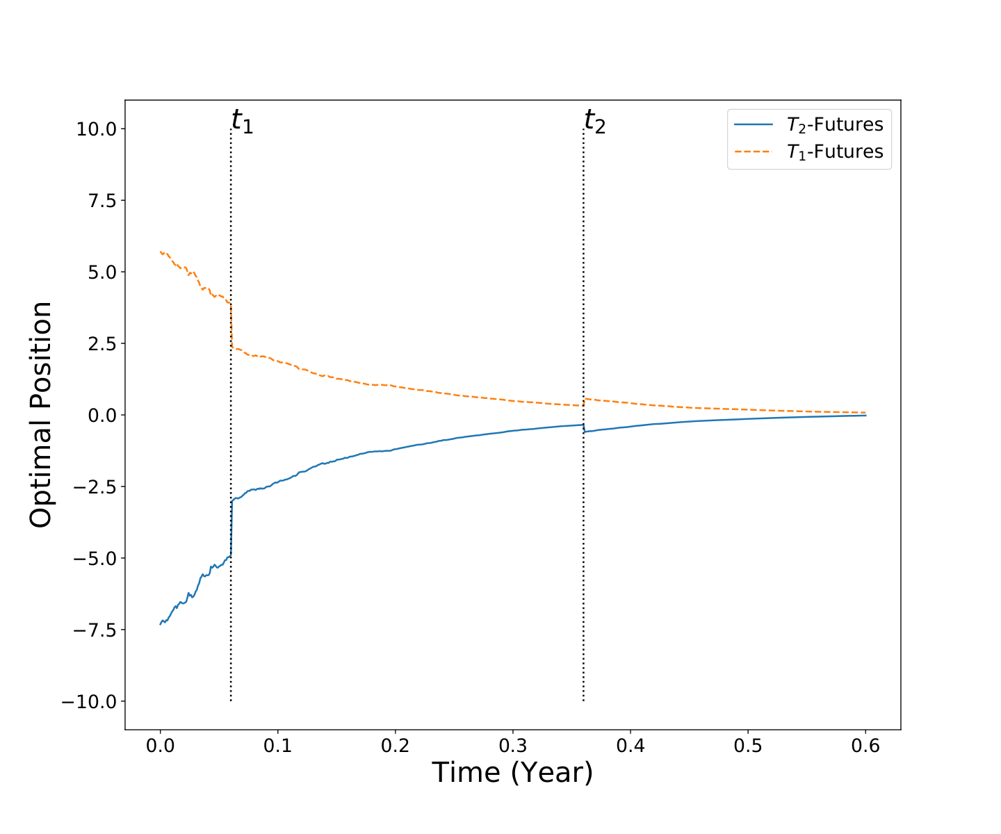
In Figure 3, we illustrate the sample paths of the optimal positions in the two futures over the trading horizon. As we can see, the optimal positions are of opposite signs, meaning that the investor will go long on the T1T_{1}-Futures and short on the T2T_{2}-Futures. Long-short strategies are very common in futures trading, and they can help mitigate the effect of regime switching. As the market switches from regime 2 to regime 1 at time t1t_{1}, the magnitude of the futures position is reduced immediately. The investor then take larger long-short positions when the market returns to regime 2 from regime 1 at time t2t_{2}. According to the sample paths, the optimal positions tend to decay in time during each regime, meaning that the investor gradually reduces investments towards the end of the trading horizon.

Figure 4 shows the wealth process corresponding to the optimal trading strategy in Figure 3. The long-short strategy tends to reduce the shock in portfolio vlaue due to regime switching. Therefore, no sizable jumps in the wealth process are observed at the regime-swtiching times t1t_{1} and t2t_{2}. As we can see, the wealth process decreases slightly in regime 1. This is intuitive since regime 1 has lower risk premium than in regime 2. The wealth increases sharply in regime 2 towards the end of the trading horizon, even though the positions are gradually reduced over time.

In Figure 5, we plot the sample path for the absolute value of coefficient matrix determinant |Φ||\Phi| corresponding to the sample paths of the spot and futures prices. Recall from (55), |Φ||\Phi| is exponentially increasing or decreasing overtime. Moreover, in our numerical settings, the term q~​(i,i)=−q~​(i,j)\tilde{q}(i,i)=-\tilde{q}(i,j) dominates the term μi+σi2/2\mu_{i}+\sigma_{i}^{2}/2. Therefore, |Φ||\Phi| appears to be exponentially increasing in time. Since |Φ||\Phi| is not equal to 0, Γ\Gamma is invertible and we are able to apply the results in the Section 3 for the RS-GBM model.

Refer to caption
Figure 2: Sample paths of the spot price, T1T_{1}-futures price, and T2T_{2}-futures price over the trading horizon under the RS-GBM model. The market starts in regime 2, then switches to regime 1 at time t1t_{1}, before switching back to regime 2 at time t2t_{2}.
Refer to caption
Figure 3: Sample paths of the optimal positions (π(1),π(2)\pi^{(1)},\pi^{(2)}) in the T1T_{1}-futures and T2T_{2}-futures respectively under the RS-GBM model. The futures positions tend to decrease over time and approaches zero near the end of the trading horizon. Jumps in both positions occur at the regiem-switching times t1t_{1} and t2t_{2}.
Refer to caption
Figure 4: Sample path of the optimal wealth process over the trading horizon under the RS-GBM model.
Refer to caption
Figure 5: Sample path of the absolute value of the determinant Φ\Phi for the coefficient matrix Γ\Gamma under the RS-GBM model.

5 Regime-Switching Exponential Ornstein-Uhlenbeck Model

As is well known, the Exponential Ornstein-Uhlenbeck process and its variations are widely used to model commodity prices. We now consider the Regime-Switching Exponential Ornstein-Uhlenbeck (RS-XOU) model and illustrate the optimal trading strategies under this model. In the RS-XOU model, the log spot price evolves according to

d​Xt=κ⁡(ξt)​(θ⁡(ξt)−Xt)​d​t+σ⁡(ξt)​d​Ztℚ,dX_{t}=\kappa(\xi_{t})(\theta(\xi_{t})-X_{t})dt+\sigma(\xi_{t})dZ_{t}^{\mathbb{Q}}, (61)

where κ⁡(ξt)\kappa(\xi_{t}), θ⁡(ξt)\theta(\xi_{t}) and σ⁡(ξt)\sigma(\xi_{t}) are the functions of regimes. This amounts to setting a~​(t,Xt,ξt)=κ⁡(ξt)​(θ⁡(ξt)−Xt)\tilde{a}(t,X_{t},\xi_{t})=\kappa(\xi_{t})(\theta(\xi_{t})-X_{t}) and b⁡(t,Xt,ξt)=σ⁡(ξt)b(t,X_{t},\xi_{t})=\sigma(\xi_{t}) in (6).

5.1 Futures Dynamics and Utility Maximization

The futures price function Fi​(t,x)F_{i}(t,x) satisfies PDE (8). Substituting (61) into (15), we obtain the ℚ\mathbb{Q}-dynamics for futures price FtF_{t}:

d​Ft\displaystyle dF_{t} =η(t,Xt,ξt)dZtℚ+∫ℝ∑j∈E∖{ξt}(F(t,Xt,j)−F(t,Xt,ξt))I{z∈Δ(ξt,j)}Mℚ(dt,dz),\displaystyle=\eta(t,X_{t},\xi_{t})dZ_{t}^{\mathbb{Q}}+\int_{\mathbb{R}}\sum_{j\in E\setminus\{\xi_{t}\}}\bigg(F(t,X_{t},j)-F(t,X_{t},\xi_{t})\bigg)I_{\{z\in\Delta(\xi_{t},j)\}}M^{\mathbb{Q}}(dt,dz), (62)

where the volatility term is given by

η⁡(t,x,i)=σi​∂xFi​(t,x).\eta(t,x,i)=\sigma_{i}\partial_{x}F_{i}(t,x). (63)

In addition, under the measure ℙ{\mathbb{P}},

d​Ft\displaystyle dF_{t} =(ζ⁡(ξt)​η​(t,Xt,ξt)+∑j∈E∖{ξt}(q⁡(ξt,j)−q~​(ξt,j))​(F⁡(t,Xt,j)−F⁡(t,Xt,ξt)))​d​t\displaystyle=\bigg(\zeta(\xi_{t})\eta(t,X_{t},\xi_{t})+\sum_{j\in E\setminus\{\xi_{t}\}}(q(\xi_{t},j)-\tilde{q}(\xi_{t},j))\bigg(F(t,X_{t},j)-F(t,X_{t},\xi_{t})\bigg)\bigg)dt (64)
+η(t,Xt,ξt)dZtℙ+∫ℝ∑j∈E∖{ξt}(F(t,Xt,j)−F(t,Xt,ξt))I{z∈Δ(ξt,j)}Mℙ(dt,dz).\displaystyle+\eta(t,X_{t},\xi_{t})dZ_{t}^{{\mathbb{P}}}+\int_{\mathbb{R}}\sum_{j\in E\setminus\{\xi_{t}\}}\bigg(F(t,X_{t},j)-F(t,X_{t},\xi_{t})\bigg)I_{\{z\in\Delta(\xi_{t},j)\}}M^{\mathbb{P}}(dt,dz).
Example 4

We consider a portfolio of futures with two different maturities T1T_{1} and T2T_{2} in a two-state market, i.e. E={1,2}E=\{1,2\}. The associated coefficient matrix is given by

𝚪⁡(t,x,i)=[σi​∂xFi(1)​(t,x)σi​∂xFi(2)​(t,x)Fj(1)​(t,x)−Fi(1)​(t,x)Fj(2)​(t,x)−Fi(2)​(t,x)],\bm{\Gamma}(t,x,i)=\left[\begin{array}[]{ccccccccccccccc}\sigma_{i}\partial_{x}F^{(1)}_{i}(t,x)&\sigma_{i}\partial_{x}F^{(2)}_{i}(t,x)\\ F^{(1)}_{j}(t,x)-F^{(1)}_{i}(t,x)&F^{(2)}_{j}(t,x)-F^{(2)}_{i}(t,x)\end{array}\right], (65)

for (i,j)∈{(1,2),(2,1)}(i,j)\in\{(1,2),(2,1)\}. Moreover, we assume 𝚪⁡(t,x,i)\bm{\Gamma}(t,x,i) be invertible. Under this assumption, we can apply the result in Section 3. The value function ui​(t,w)=−e−γ​w+φi​(t)u_{i}(t,w)=-e^{-\gamma w+\varphi_{i}(t)}, where φi​(t)\varphi_{i}(t) is given by (36), holds.

Applying (37), we immediately obtain the optimal strategy

[π(1)∗i(t,x)π(2)∗i(t,x)]=−1γ​σi​((Fj(2)​(t,x)−Fi(2)​(t,x))​∂xFi(1)​(t,x)−(Fj(1)​(t,x)−Fi(1)​(t,x))​∂xFi(2)​(t,x))\displaystyle\left[\begin{array}[]{ccccccccccccccc}\pi^{(1)*}_{i}(t,x)\\ \pi^{(2)*}_{i}(t,x)\end{array}\right]=-\frac{1}{\gamma\sigma_{i}((F^{(2)}_{j}(t,x)-F^{(2)}_{i}(t,x))\partial_{x}F^{(1)}_{i}(t,x)-(F^{(1)}_{j}(t,x)-F^{(1)}_{i}(t,x))\partial_{x}F^{(2)}_{i}(t,x))} (66)
[−ζi​(Fj(2)​(t,x)−Fi(2)​(t,x))−σi​∂xFj(2)​(t,x)​(log⁡λ~iλi+φi​(t)−φj​(t))ζi​(Fj(1)​(t,x)−Fi(1)​(t,x))+σi​∂xFj(1)​(t,x)​(log⁡λ~iλi+φi​(t)−φj​(t))],\displaystyle\left[\begin{array}[]{ccccccccccccccc}-\zeta_{i}(F_{j}^{(2)}(t,x)-F_{i}^{(2)}(t,x))-\sigma_{i}\partial_{x}F_{j}^{(2)}(t,x)(\log\frac{\tilde{\lambda}_{i}}{\lambda_{i}}+\varphi_{i}(t)-\varphi_{j}(t))\\ \zeta_{i}(F_{j}^{(1)}(t,x)-F_{i}^{(1)}(t,x))+\sigma_{i}\partial_{x}F_{j}^{(1)}(t,x)(\log\frac{\tilde{\lambda}_{i}}{\lambda_{i}}+\varphi_{i}(t)-\varphi_{j}(t))\end{array}\right],

for (i,j)∈{(1,2),(2,1)}(i,j)\in\{(1,2),(2,1)\} and (t,x)∈[0,T~]×ℝ(t,x)\in[0,\tilde{T}]\times{\mathbb{R}}.

Remark 5

If the speed of mean reversion is identical in all regimes, i.e. κi=κ\kappa_{i}=\kappa ∀i\forall i, then the futures price admits the following form

Fi​(t,x)=exp⁡(e−κ⁡(T−t)​x)​hi​(t),F_{i}(t,x)=\exp\bigg(e^{-\kappa(T-t)}x\bigg)h_{i}(t), (67)

where (hi​(t))i=1,…,M(h_{i}(t))_{i=1,\ldots,M} solves the ODE system

hi′​(t)+(κ​θi​e−κ⁡(T−t)+σi22​e−2​κ​(T−t))​hi​(t)+∑j∈E∖{i}q~​(i,j)​(hj​(t)−hi​(t))=0,\displaystyle h^{\prime}_{i}(t)+\bigg(\kappa\theta_{i}e^{-\kappa(T-t)}+\frac{\sigma^{2}_{i}}{2}e^{-2\kappa(T-t)}\bigg)h_{i}(t)+\sum_{j\in E\setminus\{i\}}\tilde{q}(i,j)(h_{j}(t)-h_{i}(t))=0, (68)

with the terminal condition hi​(T)=1h_{i}(T)=1, for i=1,…,Mi=1,\ldots,M.

The price formula (67) means that η⁡(t,x,i)=σi​e−κ⁡(T−t)​Fi​(t,x)\eta(t,x,i)=\sigma_{i}e^{-\kappa(T-t)}F_{i}(t,x) in (15). As a result, the futures price satisfies the SDE

d​Ft\displaystyle dF_{t} =σ⁡(ξt)​e−κ⁡(T−t)​exp⁡(e−κ⁡(T−t)​Xt)​h​(t,ξt)​d​Ztℚ\displaystyle=\sigma(\xi_{t})e^{-\kappa(T-t)}\exp\bigg(e^{-\kappa(T-t)}X_{t}\bigg)h(t,\xi_{t})dZ_{t}^{\mathbb{Q}} (69)
+exp(e−κ⁡(T−t)Xt)∫ℝ∑j∈E∖{ξt}(h(t,j)−h(t,ξt))I{z∈Δ(ξt,j)}Mℚ(dt,dz),\displaystyle+\exp\bigg(e^{-\kappa(T-t)}X_{t}\bigg)\int_{\mathbb{R}}\sum_{j\in E\setminus\{\xi_{t}\}}\bigg(h(t,j)-h(t,\xi_{t})\bigg)I_{\{z\in\Delta(\xi_{t},j)\}}M^{\mathbb{Q}}(dt,dz),

where we have denoted h⁡(t,i)≡hi​(t)h(t,i)\equiv h_{i}(t).

5.2 Numerical Method for Futures Price

We now discuss the numerical procedue to compute the futures price under the RS-XOU model in this section. We have computed and checked our prices using the finite difference method (FDM) and fast fourier transform (FFT).

5.2.1 Finite Difference Method (FDM)

We first re-write futures price PDE (8) in terms of s=exs=e^{x} to get

∂tFi+(κi​(θi−ln⁡s)+σi22)​s​∂sFi+σi2​s22​∂s​sFi+∑j∈E∖{i}q~​(i,j)​(Fj−Fi)=0,\displaystyle\partial_{t}F_{i}+\bigg(\kappa_{i}(\theta_{i}-\ln s)+\frac{\sigma_{i}^{2}}{2}\bigg)s\partial_{s}F_{i}+\frac{\sigma^{2}_{i}s^{2}}{2}\partial_{ss}F_{i}+\sum_{j\in E\setminus\{i\}}\tilde{q}(i,j)(F_{j}-F_{i})=0, (70)

for (t,s)∈[0,T)×ℝ+(t,s)\in[0,T)\times{\mathbb{R}}_{+}, with the terminal condition Fi​(T,s)=sF_{i}(T,s)=s. Then we can apply the Crank-Nicolson method to equation (70) directly with Dirichlet boundary conditions. The method is standard, so we omit the details here.

5.2.2 Fourier Space Time-stepping (FST)

We begin first by discretizing the continuous-time Markov chain ξt\xi_{t} with time step of size δ​t\delta t, and we keep ξt\xi_{t} constant on each time interval (tn,tn+1](t_{n},t_{n+1}] (tn=n​δ​t)(t_{n}=n\delta t), for n=0,…,T/δ​t−1n=0,\ldots,T/\delta t-1, with transition probabilities

Pk​l:={1+q~l​l​δ​t,k=l,q~k​l​δ​t,o​t​h​e​r​w​i​s​e.P_{kl}:=\left\{\begin{aligned} &1+\tilde{q}_{ll}\delta t,&k=l,\\ &\tilde{q}_{kl}\delta t,&otherwise.\end{aligned}\right. (71)

In turn, the futures price satisfies the recursive relation

Fi​(tn,x)=∑j=1,…,MPi​j​Fj​(tn+,x),F_{i}(t_{n},x)=\sum_{j=1,\ldots,M}P_{ij}F_{j}(t_{n+},x), (72)

where Fj​(tn+,x)=limt↓tnFj​(t,x)F_{j}(t_{n+},x)=\lim_{t\downarrow t_{n}}F_{j}(t,x).

Since we assume Markov chain ξt\xi_{t} stay constant on time intervals (tn,tn+1](t_{n},t_{n+1}], the martingale property of futures price implies that

Fi​(tn+,x)=I​Eℚ​[Fi​(tn+1,Xtn+1)|Xtn=x],F_{i}(t_{n+},x)={{\mathord{I\kern-3.30002ptE}}}^{\mathbb{Q}}[F_{i}(t_{n+1},X_{t_{n+1}})|X_{t_{n}}=x], (73)

for i=1,…,Mi=1,\ldots,M, and n=0,…,T/δ​t−1n=0,\ldots,T/\delta t-1. Therefore, we have following PDE for the futures price within each time interval (tn,tn+1](t_{n},t_{n+1}] and regime ii,

∂tFi+κi​(θi−x)​∂xFi+σi22​∂x​xFi=0.\displaystyle\partial_{t}F_{i}+\kappa_{i}(\theta_{i}-x)\partial_{x}F_{i}+\frac{\sigma^{2}_{i}}{2}\partial_{xx}F_{i}=0. (74)

Next, we apply Fourier transform to PDE (74). To that end, we define

ℱ⁡[f]​(ω)=∫−∞∞f⁡(x)​exp⁡(−j​ω​x)​𝑑x,{\mathcal{F}}[f](\omega)=\int_{-\infty}^{\infty}f(x)\exp(-j\omega x)dx, (75)

where jj denotes the imaginary identity and ω\omega denotes the frequency. Then, we obtain a first-order PDE for F^:=ℱ⁡[F]\hat{F}:={\mathcal{F}}[F]:

∂F^i+κi​ω​∂^ω​Fi+(κi​θi​j​ω+κi−ω2​σi22)​F^i=0,\partial\hat{F}_{i}+\kappa_{i}\omega\hat{\partial}_{\omega}F_{i}+\bigg(\kappa_{i}\theta_{i}j\omega+\kappa_{i}-\frac{\omega^{2}\sigma_{i}^{2}}{2}\bigg)\hat{F}_{i}=0, (76)

for (t,ω)∈[0,T)×ℝ(t,\omega)\in[0,T)\times\mathbb{R}, where F^​(t,ω)≡ℱ⁡[F]​(t,ω)\hat{F}(t,\omega)\equiv{\mathcal{F}}[F](t,\omega). Noted that we use the following property of the Fourier transform to derive PDE (76),

ℱ⁡[x​fx]=−ℱ⁡[f]−ω​ℱω​[f].{\mathcal{F}}[xf_{x}]=-{\mathcal{F}}[f]-\omega{\mathcal{F}}_{\omega}[f]. (77)

To solve PDE (76) we employ the method of characteristics to get

F^i​(tn+,ω)=ϕi​(δ​t,ω)​F^i​(tn+1,eκi​δ​t​ω),\displaystyle\hat{F}_{i}(t_{n}+,\omega)=\phi_{i}(\delta t,\omega)\hat{F}_{i}(t_{n+1},e^{\kappa_{i}\delta t}\omega), (78)

with

ϕi​(δ​t,ω)=exp⁡(κi​δ​t−θi​j​ω​(1−eκi​δ​t)+σi2​ω24​κi​(1−e2​κi​δ​t)).\phi_{i}(\delta t,\omega)=\exp\bigg(\kappa_{i}\delta t-\theta_{i}j\omega(1-e^{\kappa_{i}\delta t})+\frac{\sigma_{i}^{2}\omega^{2}}{4\kappa_{i}}(1-e^{2\kappa_{i}\delta t})\bigg).

Combining equation (72) and (78), we have following backward equation in the frequency space,

F^i​(tn,ω)=∑j=1,…,MPi​j​ϕj​(δ​t,ω)​F^j​(tn+1,eκj​δ​t​ω),\hat{F}_{i}(t_{n},\omega)=\sum_{j=1,\ldots,M}P_{ij}\phi_{j}(\delta t,\omega)\hat{F}_{j}(t_{n+1},e^{\kappa_{j}\delta t}\omega), (79)

for i=1,…,Mi=1,\ldots,M, and n=0,…,T/δ​t−1n=0,\ldots,T/\delta t-1. We then apply backward induction via (79) to calculate F^i​(t,ω)\hat{F}_{i}(t,\omega). To recover the original futures price function, we apply inverse Fourier transform. For the numerical implementation of Fourier transform and inverse Fourier transform, we utilize the standard fast Fourier transform algorithm. This FST method has been applied more broadly by Jackson et al. 2008 to solve partial-integro differential equations (PIDEs) that arise in options pricing problems. For more details and other applications of this numerical approach, we refer to Surkov 2009 and Jackson et al. 2008, and references therein.

5.3 Numerical Example

We simulate the sample paths for spot price, futures prices, optimal investment, and optimal wealth process. The regime switching between two states, with transition probabilities q12=2q_{12}=2 and q21=4q_{21}=4 which are entries of generator matrix 𝑸\bm{Q}. The trading horizon T~=0.6\tilde{T}=0.6, and the two futures contracts have maturities T1=0.6T_{1}=0.6 and T2=0.8T_{2}=0.8. All parameters are summarized in the Table 2.

q~12=q12\tilde{q}_{12}=q_{12} q~21=q21\tilde{q}_{21}=q_{21} ζ⁡(1)\zeta(1) ζ⁡(2)\zeta(2) κ1\kappa_{1} κ2\kappa_{2} γ\gamma
22 44 0.1 0.3 1 2 1
θ1\theta_{1} θ2\theta_{2} σ1\sigma_{1} σ2\sigma_{2} T1T_{1} T2T_{2} T~\tilde{T}
2.5 2.7 0.2 0.3 0.6 0.8 0.6
Table 2: Parameters for the RS-XOU model for Figures 6–9.

For the sample paths shown in Figure 6, the market starts in regime 2, then switches to regime 1 at time t1t_{1}) before returning to regime 2 at time t2t_{2}. The two price levels exp⁡(θ1)\exp(\theta_{1}) and exp⁡(θ2)\exp(\theta_{2}) are the long-run means of the spot price in regimes 1 and 2 respectively. In each regime, the spot price tends to move towards the corresponding mean level. The spot and futures prices tend to move in tandem. Nevertheless, like in Figure 2, each regime switch can cause an instant jump in the futures price but not in the spot price.

Figure 7 shows the sample path of the optimal positions in the two futures over the trading horizon. The optimal strategy is to long T1T_{1}-Futures and short T2T_{2}-Futures. The long-short positions help reduce the effect of regime switching. As the market switches from regime 2 to regime 1 at time t1t_{1}, the magnitude of the futures position is immediately reduced. The investor then take larger positions when the market returns to regime 2 from regime 1 at time t2t_{2}. According to the sample paths, the optimal positions tend to decay in time during each regime, meaning that the investor gradually reduces investments towards the end of the trading horizon.

Figure 8 shows the optimal wealth process over time. By placing opposite position in two futures, we reduce the shock in portfolio vlaue due to regime switching. Therefore, we do not observe sizable jumps in the wealth process at the regime-swtiching times t1t_{1} and t2t_{2}. Just like the futures and spot prices, the wealth process tends to decrease in regime 1 and increase in regime 2 (towards the end of the trading horizon).

Lastly in Figure 9, we plot the sample path for |Φ||\Phi|, which is the absolute value of coefficient matrix determinant Γ\Gamma. The strict positivity of |Φ||\Phi| informs us that Γ\Gamma is invertible and thus the results in Section 3 can be applied. Like in Figure 5, |Φ||\Phi| tends to increase exponentially in time.

Refer to caption
Figure 6: Sample paths of the spot price, T1T_{1}-futures price, and T2T_{2}-futures price over the trading horizon under the RS-XOU model. The market starts in regime 2, then switches to regime 1 at time t1t_{1}, before switching back to regime 2 at time t2t_{2}.
Refer to caption
Figure 7: Sample paths of the optimal positions (π(1),π(2)\pi^{(1)},\pi^{(2)}) in the T1T_{1}-futures and T2T_{2}-futures respectively under the RS-XOU model. The futures positions tend to decrease over time and approaches zero near the end of the trading horizon. Jumps in both positions occur at the regiem-switching times t1t_{1} and t2t_{2}.
Refer to caption
Figure 8: Sample path of the optimal wealth process over the trading horizon under the RS-XOU model.
Refer to caption
Figure 9: Sample path of the absolute value of the determinant Φ\Phi for the coefficient matrix Γ\Gamma under the RS-XOU model.

6 Conclusion

We have analyzed the problem of dynamically trading a portfolio of futures in a regime-switching market. Under a general market framework, the portfolio optimization problem leads to the analytical and numerical studies of a system of HJB equations, which are solved explicitly. The optimal trading strategies and optimal wealth process are also given analytically and illustrated numerically. Our methodology has been applied to the RS-GBM and RS-XOU models, but it can also be used for other model specifications within the framework or adapted to study models with additional factors. Moreover, one can also utilize our framework to examine other classes of trading strategies, such as rolling and timing strategies.22 2 See Leung and Li 2016 and Leung et al. 2016 for such strategies under mean-reverting models. Other than futures portfolio, it is also useful to study the dynamic trading of other derivatives, such as options and swaps, in a regime-switching market.

References

  • Angoshtari and Leung (2019a) Angoshtari, B. and Leung, T. (2019a). Optimal dynamic basis trading. Annals of Finance, 15(3):307–335.
  • Angoshtari and Leung (2019b) Angoshtari, B. and Leung, T. (2019b). Optimal trading of a basket of futures contracts. Working Paper. Available at https://ssrn.com/abstract=3467897.
  • Buffington and Elliott (2002) Buffington, J. and Elliott, R. J. (2002). American options with regime switching. International Journal of Theoretical and Applied Finance, 5:497–514.
  • Chen et al. (2019) Chen, K., Chiu, M., and Wong, H. (2019). Time-consistent mean-variance pairs-trading under regime-switching cointegration. SIAM Journal on Financial Mathematics, 10(2):632–665.
  • Elliott et al. (2005) Elliott, R. J., Chan, L., and Siu, T. K. (2005). Option pricing and Esscher transform under regime switching. Annals of Finance, 1(4):423– 432.
  • Jackson et al. (2008) Jackson, K. R., Jaimungal, S., and Surkov, V. (2008). Fourier space time-stepping for option pricing with Lévy models. Journal of Computational Finance, 12(2):1–29.
  • Leung (2010) Leung, T. (2010). A markov-modulated stochastic control problem with optimal stopping with application to finance. In Proceedings of the 49th IEEE Conference on Decision and Control.
  • Leung et al. (2016) Leung, T., Li, J., Li, X., and Wang, Z. (2016). Speculative futures trading under mean reversion. Asia-Pacific Financial Markets, 23(4):281–304.
  • Leung and Li (2016) Leung, T. and Li, X. (2016). Optimal Mean Reversion Trading: Mathematical Analysis and Practical Applications. Modern Trends in Financial Engineering. World Scientific Publishing Company.
  • Leung and Yan (2018) Leung, T. and Yan, R. (2018). Optimal dynamic pairs trading of futures under a two-factor mean-reverting model. International Journal of Financial Engineering, 5(3):1850027.
  • Leung and Yan (2019) Leung, T. and Yan, R. (2019). A stochastic control approach to managed futures portfolios. International Journal of Financial Engineering, 6(1):1950005.
  • Merton (1971) Merton, R. (1971). Optimum consumption and portfolio rules in a continuous time model. Journal of Economic Theory, 03:373–413.
  • Surkov (2009) Surkov, V. (2009). Option Pricing Using Fourier Space Time-Stepping Framework. PhD thesis, University of Toronto.
  • Zhou and Yin (2003) Zhou, X. and Yin, G. (2003). Markowitz’s mean-variance portfolio selection with regime switching: A continuous-time model. SIAM Journal on Control and Optimization, 42(4):1466–1482.