Measurements of electric quadrupole transition frequencies in 226Ra+
Abstract
We report the first driving of the and electric quadrupole (E2) transitions in Ra+. We measure the frequencies of both E2 transitions, and two other low-lying transitions in 226Ra+ that are important for controlling the radium ion’s motional and internal states: and .
I Introduction
The radium ion has two subhertz-linewidth electric quadrupole (E2) transitions from the ground state: at 728 nm and at 828 nm. The E2 transition to the state, which has a lifetime of 300 ms Pal et al. 2009, is useful for electron shelving, ground-state cooling, and controlling an optical qubit, and it could also serve as the clock transition for an optical clock Nuñez Portela et al. 2014. Measurement of these two quadrupole transitions across a chain of isotopes can be used to obtain information related to the nuclear structure of radium, such as the specific mass shift and the change in mean-square nuclear charge radii Heilig and Steudel 1974; Reinhard et al.. The degree of nonlinearity in a King plot comparison of the two transitions could set bounds on new physics beyond the standard model Berengut et al. 2018. There are 11 radium isotopes between mass number 213 and mass number 234 with half-lives longer than 1 min that could be ionized, trapped, and compared with a high precision on a King plot. A precision King plot can also be made using one E2 transition in Ra+ and the Ra intercombination line at 765 nm, which has a mHz linewidth Bieroń et al. 2007.
In this work we measure the two electric quadrupole transition frequencies, as well as the frequencies of the (708-nm) and (802-nm) electric dipole transitions (see Fig. 1) in 226Ra+ (, 1600 yr half-life). Previously the only optical frequency measurement in 226Ra+ with an uncertainty of less than is that of the (468-nm) Doppler cooling transition Fan et al. 2019. Combining that measurement with the measurements in this work, we calculate the (1079-nm) and (382-nm) frequencies, which are useful for laser-cooling Ra+.
For our measurements we use a single laser-cooled radium ion, which is loaded by ablating a 10 Ci RaCl2 target from the trap. The radio-frequency trapping voltage is turned on after ablation to enhance the loading efficiency. The radium ion trap and loading procedure used in this work have been described previously Fan et al. 2019. We use a heated iodine vapor cell as a frequency reference. The Ra+ spectroscopy transitions and the iodine reference are driven with a tunable Ti:sapphire laser, whose frequency is recorded with a wave meter (High Finesse WS-8) to determine the Ra+ transition frequencies from the known iodine reference lines. We describe the Ra+ transition measurements and fits in Sec. II, and the iodine frequency reference spectroscopy in Sec. III. From the combined iodine and Ra+ data we determine the Ra+ transition frequencies in Sec. IV, and with these values we present an updated King plot that includes radium-226 in Sec. V.
II Radium Spectroscopy
The Ra+ transitions are measured using state detection, where the ion is bright if the population is in the cooling cycle and dark otherwise. Bright-state fluorescence photons at 468 nm are collected onto a photomultiplier tube and the counts are then time-tagged with respect to the measurement pulse sequences Pruttivarasin and Katori 2015. In 1 ms of state detection 35 photons are collected on average if the population is in the or “bright” state, and 1.5 photons of background scattered light if the population is shelved in the “dark” state. We set the bright-state detection threshold to 12 counts.

All Ra+ spectroscopy pulse sequences begin with 0.5 ms of laser cooling and an initial state detection (see SD1 in Fig. 2). If the state detection finds the ion in the dark state, then the data point is excluded because the ion is not properly initialized. All pulse sequences finish with a second state detection step and then optical pumping to remove any remaining population from the state. We give a detailed description of the electric quadrupole “clock” transition measurement. The other measurements are similar, with brief descriptions provided.
II.1 (728 nm)
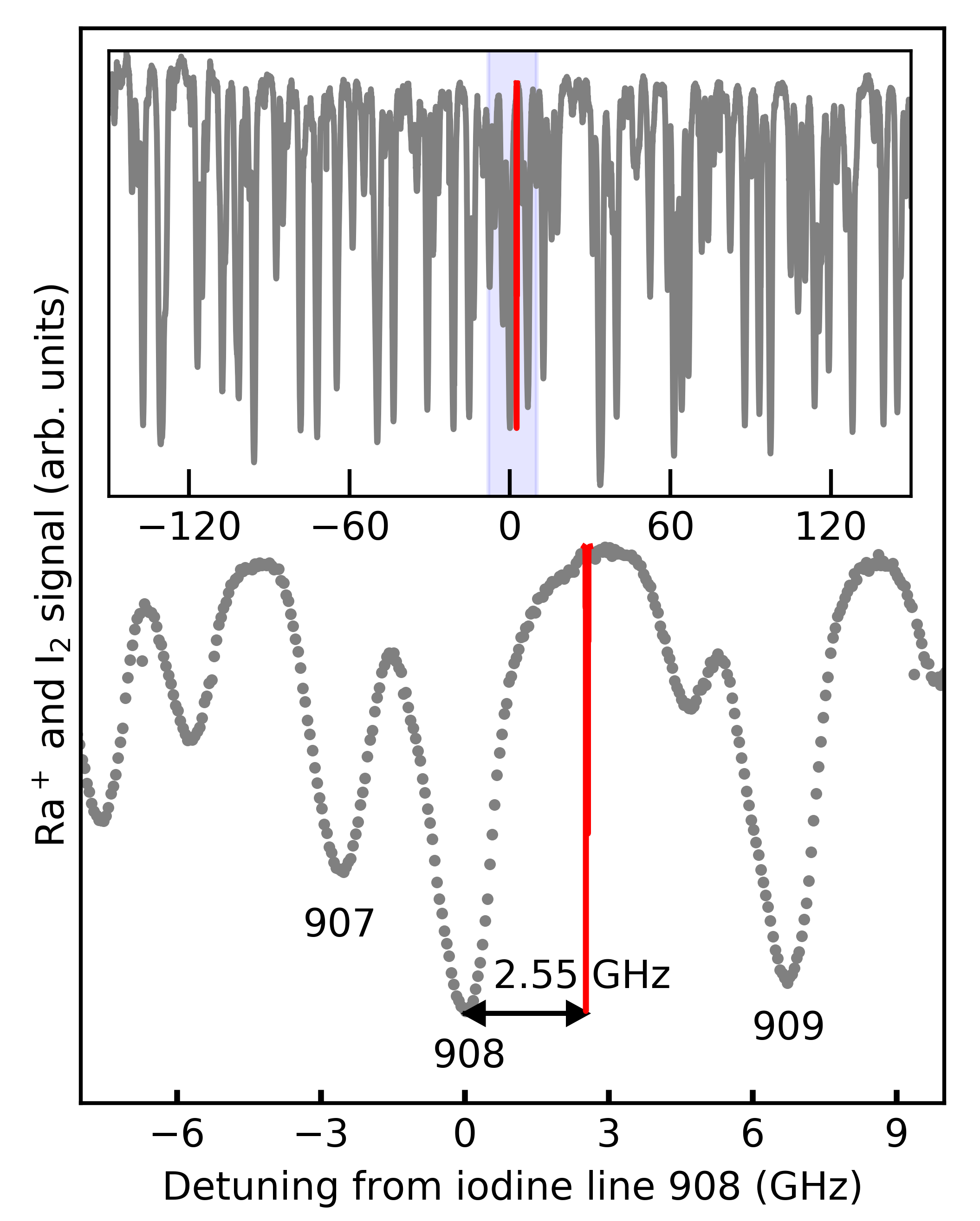
The pulse sequence for the clock transition measurement is shown in Fig. 2. Before each measurement we Doppler-cool the ion for 0.5 ms. The initial state detection determines whether the ion is cooled, and whether the population is in a bright state (SD1). Any population in the state is then optically pumped with light at 1079 nm to the ground state (P1). The spectroscopy transition is then driven with light at 728 nm for 1 ms (P2), and if the light is on resonance, the population can be shelved to the state, and the shelving probability is measured with a second state detection (SD2). To prepare for the next measurement any shelved population is cleaned out with light at 802 nm, which drives the population to the and bright states (P3). Over many pulse sequences the 728-nm laser is swept over to drive all possible transitions between Zeeman levels of the two states. The spectroscopy is shown in Fig. 3, along with an inset of the corresponding iodine absorption reference spectrum.


To resolve the and Zeeman sub-structure of the transitions, a 7.8-G magnetic field is applied parallel to the trap’s radio-frequency rods, which we define as the axis. The magnetic field spreads the transitions across . The energy splitting due to the applied magnetic field is calculated from , where is the Landé -factor for state with total angular momentum , is the Bohr magneton, is the magnetic field, and is the magnetic quantum number. The Rabi frequency for transitions between the and the Zeeman levels is
| (1) | ||||
where is the reduced matrix element, the summation is over Wigner 3- symbols and a geometry-dependent factor, James 1998; Roos 2000, given by
| (2) | ||||
where is the change in magnetic quantum number, is the angle between the laser’s vector and the magnetic field, and is the angle between the laser polarization and the magnetic field vector projected into the plane of incidence.
For E2 transitions are allowed, which gives rise to 10 transitions between Zeeman levels for . We measure these transitions using , and two values of , and , which suppress certain transitions (see Fig. 4). We fit the spectroscopy data to a sum of 10 Lorentzians, from which we extract the applied magnetic field, , , and the transition frequency. Due to the 468- and 1079-nm laser polarizations, during Doppler cooling the ground-state level is preferentially populated, and so reduces the probability of transition occurring from the level. The ground state population imbalance is one of the fitting parameters. The 0.5-Hz natural linewidth of the transition is broadened by laser power and magnetic field fluctuations. There are small micromotion sidebands in the spectrum at our trap drive frequency, . We average the two center frequencies extracted from the two fits of the spectra at different values of to determine the transition frequency.

II.2 (802 nm)
For measuring both the and the transitions a magnetic field of 2.5 G is applied to prevent coherent dark states Berkeland and Boshier 2002. After initialization, the ion is optically pumped to the state with light at 468 and 708 nm for . Any population in the state is then pumped with the spectroscopy light at 802 nm for . If the light is on resonance, the population can be driven to the state, where decays will populate the bright states (see Fig. 5). After the second state detection the state is optically pumped with resonant 802-nm light from an external cavity diode laser.
To determine the line center for the transition we fit the data to a Lorentzian (see Fig. 5). The full width at half-maximum (FWHM) of gives a lower bound of for the -state lifetime, which agrees with the calculated value of Pal et al. 2009. The 802-nm laser light is incident on the ion along the trap’s z axis to minimize micromotion broadening Berkeland et al. 1998. We measured the 802-nm laser’s beam waist to be and our beam power to be . We estimate that the transition is power broadened by from the 802-nm beam waist and power.
II.3 (828 nm)
After initialization, any population in the state is optically pumped with light at 1079 nm for to the ground state. The transition is driven with light at 828 nm for 10 ms, and if the light is on resonance, the ion can be shelved to the state. Any population in the state is then pumped with light at 708 nm for , which drives the population to the state whose decays populate the and states.
The population is shelved to the state with a low fidelity due to the branching fraction from the state. The shelved probability is determined from a binomial distribution of shelved events (corresponding to fewer than 12 photons collected during the second state detection) in trials (where the ion is properly initialized at the beginning of the pulse sequence). There are eight transitions between Zeeman levels for the transition. We fit the spectra in a similar fashion as the transition to extract the center frequency.
II.4 (708 nm)
After initialization, any population in the state is optically pumped with light at 468 nm for to the state. The population is then pumped with light at 708 nm for , and if the light is on resonance, the population can be driven to the state whose decays populate the and bright states. The data are fit to a Lorentzian to determine the center frequency.
III Iodine Frequency Reference
For iodine absorption spectroscopy the Ti:sapphire laser is scanned at 10 MHz per second across a frequency range that includes at least two iodine reference lines, as well as the target Ra+ transition. To reduce drift in the wave meter measurement we measure the iodine spectra both before and after Ra+ spectroscopy. We use one iodine line as the frequency reference, and we determine the line’s frequency by fitting the line’s absorption dip in both scans to a Voigt function and averaging the two centers. We then calibrate the iodine line frequency we measured with a wave meter to an absolute frequency using IodineSpec5 Iod; Knöckel et al. 2004, which provides a comprehensive I2 reference data set based on iodine spectrum measurements including the original iodine atlas work Gerstenkorn 1982; *Gerstenkorn1982a. We fit the corresponding absorption dip in the IodineSpec5 data set to a Voigt function to determine the absolute frequency of the measured iodine line center.
The 127I2 vapor cell frequency reference (75 mm long, with a 19-mm outer diameter and windows angled at 11∘) is heated in a tube furnace to 500C, the temperature at which the iodine atlas lines were measured Gerstenkorn 1982; *Gerstenkorn1982a. We scan the temperature of the I2 cell by C around 500C and vary an applied magnetic field by G, and for both we find frequency shifts within the fitting uncertainty. To compensate for laser power drifts the power is recorded on a reference photodiode before the iodine cell.
IV Ra Transition Frequencies
The Ra+ transition frequencies are calculated from the frequency difference between the radium and the iodine reference line centers that are recorded with a wave-meter. The fit iodine reference lines calculated in IodineSpec5 are used to calibrate the wave-meter frequencies.
The closest iodine reference line to the transition is line 908 from Gerstenkorn 1982; Gerstenkorn and Luc 1982, which we calculate using IodineSpec5 to be . From the difference between radium and iodine spectroscopy center fits, , we determine a transition frequency of . We take the total uncertainty in our measurements to be , where is the radium fitting uncertainty, is the measured iodine fitting uncertainty, is the IodineSpec5 line uncertainty, and is the wavemeter uncertainty, 10 MHz. The IodineSpec5 line uncertainties range from 2 to 45 MHz for the lines referenced in this work. The IodineSpec5 fitting uncertainties are on the kilohertz level and are negligible compared to the other uncertainties.
| Transition | Rasmussen 1933 | Nuñez Portela et al. 2014 | This work, Fan et al. 2019 |
|---|---|---|---|
| * | * | ||
| * | Fan et al. 2019 | ||
| † | |||
| † | * |
The reported value for the transition, , comes from the frequency difference between the E2 transition measured in this work and the measurement of the transition by Fan, et al. Fan et al. 2019.
From our measurements we can calculate the (382-nm) transition frequency by summing either the 728- and 802-nm frequencies, , or the 828- and 708-nm frequencies, . Both pairs of transitions originate in the ground state and end in the state. The two calculated frequencies are in good agreement, and we report the value calculated from the 728- and 802-nm frequencies, as the uncertainty in the underlying measurements is smaller. The measured and calculated frequencies are summarized in Table 1.
There are discrepancies between the transition frequencies measured in this work and those reported by Nunez, et al. Nuñez Portela et al. 2014 (see Table 1). We are able to resolve some of the discrepancies by redoing the analysis in Nuñez Portela et al. 2014. The transition frequency reported in Nuñez Portela et al. 2014, , is extrapolated from a King plot with data from Giri et al. Giri et al. 2011. From the 1079 nm/482 nm King plot (Fig. 4 in Giri et al. 2011) we find a slope of and a -intercept of amu, which gives the transformed isotope shift [see Eq. (4) below] of 54.5(1.3) amu and the transition frequency in 226Ra+ of . This value agrees with our measurement. The transition frequency reported in Nuñez Portela et al. 2014 is calculated from the frequency difference between the and the transitions. With the recalculated value of the frequency, the transition frequency is , which is also in agreement with our measurement. There remains the discrepancy between the frequency measured in this work and the value reported in Nuñez Portela et al. 2014. This discrepancy could be resolved by direct spectroscopy of the S1/2-to- transition in one of many radium isotopes, including isotope(s) 212, 214, or 221-226 Neu et al. 1989.
V King Plot

We determine isotope shifts for the 708- and 1079-nm transitions in 226Ra+. The isotope shift between a target and a reference isotope is , where is the target isotope nuclear mass, is the reference isotope nuclear mass, and is the transition frequency. We use 214Ra+, which has a closed neutron shell, as the reference isotope Wendt et al. 1987. The 1079-nm 214Ra+ reference frequency is Giri et al. 2011 and the 708-nm 214Ra+ reference frequency is Versolato et al. 2010. Isotope shifts of 468, 708, and 1079 nm are listed in Table 2. The isotope shift is parameterized as
| (3) |
where and are the normal and specific mass shifts, is the field shift, and is the Seltzer moment, which to lowest order is the difference in mean square nuclear charge radii, Heilig and Steudel 1974. The transformed isotope shift is
| (4) |
from which the ratio of field shifts between transitions and the difference in specific mass shifts can be determined King 1963. King plot comparisons of the transformed isotopes shifts give the Ra+ field shift ratios, and , which are summarized in Table 3. The 1079 nm/468 nm King plot is shown in Fig. 6.
| Isotope | 468 nm | 708 nm | 1079 nm |
|---|---|---|---|
| 210 | 8449(6) | -1884(16) | |
| 211 | 7770(4) | -1755(14) | |
| 212 | 4583(3) | -701(20) | -1025(12) |
| 213 | 3049(3) | -453(34) | -707(14) |
| 214 | 0 | 0 | 0 |
| 226 | * | * |
| FS Ratio | Theory Wansbeek et al. 2012 | Experiment Wansbeek et al. 2012 | This work |
|---|---|---|---|
| -0.16(1) | -0.136(57) | -0.171(3) | |
| -0.23(2) | -0.244(11) | -0.235(2) |
VI Conclusion
The first driving of the 728- and 828-nm electric quadrupole transitions in Ra+ lays the groundwork for quantum information science and precision measurement experiments with Ra+. Isotope shift spectroscopy of Ra+ dipole transitions has been done at the ISOLDE facility at CERN, and could be extended to a high precision by trapping Ra+ and measuring the E2 transitions Lynch et al. 2018. Estimates for the nonlinearities of a King plot of radium’s two narrow linewidth transitions following Flambaum et al. 2018 could guide searches to constrain new physics.
We thank A. Vutha and R. Ruiz for feedback on the manuscript and acknowledge support from NSF Grant No. PHY-1912665 and the Office of the President, University of California (Grant No. MRP-19-601445).
References
- Pal et al. (2009) R. Pal, D. Jiang, M. S. Safronova, and U. I. Safronova, Phys. Rev. A 79, 062505 (2009).
- Nuñez Portela et al. (2014) M. Nuñez Portela, E. A. Dijck, A. Mohanty, H. Bekker, J. E. van den Berg, G. S. Giri, S. Hoekstra, C. J. G. Onderwater, S. Schlesser, R. G. E. Timmermans, O. O. Versolato, L. Willmann, H. W. Wilschut, and K. Jungmann, Applied Physics B 114, 173 (2014).
- Heilig and Steudel (1974) K. Heilig and A. Steudel, Atomic Data and Nuclear Data Tables 14, 613 (1974).
- (4) P. G. Reinhard, W. Nazarewicz, and R. F. G. Ruiz, arXiv:1911.00699 .
- Berengut et al. (2018) J. C. Berengut, D. Budker, C. Delaunay, V. V. Flambaum, C. Frugiuele, E. Fuchs, C. Grojean, R. Harnik, R. Ozeri, G. Perez, and Y. Soreq, Phys. Rev. Lett. 120, 091801 (2018).
- Bieroń et al. (2007) J. Bieroń, P. Indelicato, and P. Jönsson, The European Physical Journal Special Topics 144, 75 (2007).
- Fan et al. (2019) M. Fan, C. A. Holliman, A. L. Wang, and A. M. Jayich, PRL 122, 223001 (2019).
- Pruttivarasin and Katori (2015) T. Pruttivarasin and H. Katori, Rev. Sci. Instrum. 86, 115106 (2015).
- Gerstenkorn (1982) V. J. C. J. Gerstenkorn, S., Atlas du spectre d’absorption de la molecule d’iode: 11000-14000 cm to the minus 1 (Laboratoire Aime-Cotton CNRS II, Paris, 1982).
- Gerstenkorn and Luc (1982) S. Gerstenkorn and P. Luc, Atlas du spectre d’absorption de la molecule d’iode: 14000-15600 cm to the minus 1 (Laboratoire Aime-Cotton CNRS II, Paris, 1982).
- James (1998) D. F. V. James, Applied Physics B 66, 181 (1998).
- Roos (2000) C. Roos, Ph.D. thesis, University of Innsbruck (2000).
- Berkeland and Boshier (2002) D. J. Berkeland and M. G. Boshier, Phys. Rev. A 65, 033413 (2002).
- Berkeland et al. (1998) D. J. Berkeland, J. D. Miller, J. C. Bergquist, W. M. Itano, and D. J. Wineland, J. Appl. Phys. 83, 5025 (1998).
- (15) H. Knöckel and E. Tiemann, IodineSpec5 (2011) (Universität Hannover, Hannover, 2011).
- Knöckel et al. (2004) H. Knöckel, B. Bodermann, and E. Tiemann, Eur. Phys. J. D 28, 199 (2004).
- Giri et al. (2011) G. S. Giri, O. O. Versolato, J. E. van den Berg, O. Böll, U. Dammalapati, D. J. van der Hoek, K. Jungmann, W. L. Kruithof, S. Müller, M. Nuñez Portela, C. J. G. Onderwater, B. Santra, R. G. E. Timmermans, L. W. Wansbeek, L. Willmann, and H. W. Wilschut, PRA 84, 020503(R) (2011).
- Rasmussen (1933) E. Rasmussen, Zeitschrift für Physik 86, 24 (1933).
- Neu et al. (1989) W. Neu, R. Neugart, E. W. Otten, G. Passler, K. Wendt, B. Fricke, E. Arnold, H. J. Kluge, and G. Ulm, Zeitschrift für Physik D Atoms, Molecules and Clusters 11, 105 (1989).
- Wendt et al. (1987) K. Wendt, S. A. Ahmad, W. Klempt, R. Neugart, E. W. Otten, and H. H. Stroke, Zeitschrift für Physik D Atoms, Molecules and Clusters 4, 227 (1987).
- Versolato et al. (2010) O. O. Versolato, G. S. Giri, L. W. Wansbeek, J. E. van den Berg, D. J. van der Hoek, K. Jungmann, W. L. Kruithof, C. J. G. Onderwater, B. K. Sahoo, B. Santra, P. D. Shidling, R. G. E. Timmermans, L. Willmann, and H. W. Wilschut, Phys. Rev. A 82, 010501(R) (2010).
- King (1963) W. H. King, J. Opt. Soc. Am. 53, 638 (1963).
- Wansbeek et al. (2012) L. W. Wansbeek, S. Schlesser, B. K. Sahoo, A. E. L. Dieperink, C. J. G. Onderwater, and R. G. E. Timmermans, Phys. Rev. C 86, 015503 (2012).
- Lynch et al. (2018) K. M. Lynch, S. G. Wilkins, J. Billowes, C. L. Binnersley, M. L. Bissell, K. Chrysalidis, T. E. Cocolios, T. D. Goodacre, R. P. de Groote, G. J. Farooq-Smith, D. V. Fedorov, V. N. Fedosseev, K. T. Flanagan, S. Franchoo, R. F. Garcia Ruiz, W. Gins, R. Heinke, î Koszorús, B. A. Marsh, P. L. Molkanov, P. Naubereit, G. Neyens, C. M. Ricketts, S. Rothe, C. Seiffert, M. D. Seliverstov, H. H. Stroke, D. Studer, A. R. Vernon, K. D. A. Wendt, and X. F. Yang, Phys. Rev. C 97, 024309 (2018).
- Flambaum et al. (2018) V. V. Flambaum, A. J. Geddes, and A. V. Viatkina, PRA 97, 032510 (2018).