Pristine IX: CFHT ESPaDOnS Spectroscopic Analysis of 115 Bright Metal-Poor Candidate Stars 2019Pristine IX: CFHT ESPaDOnS Spectroscopic Analysis of 115 Bright Metal-Poor Candidate Stars–10
Abstract
A chemo-dynamical analysis of 115 metal-poor candidate stars selected from the narrow-band Pristine photometric survey is presented based on CFHT high-resolution ESPaDOnS spectroscopy. We have discover 28 new bright (V 15) stars with [Fe/H] and 5 with [Fe/H] for success rates of 40% (28/70) and 19% (5/27), respectively. A detailed model atmospheres analysis is carried out for the 28 new metal-poor stars. Stellar parameters were determined from SDSS photometric colours, Gaia DR2 parallaxes, MESA/MIST stellar isochrones, and the initial Pristine survey metallicities, following a Bayesian inference method. Chemical abundances are determined for 10 elements (Na, Mg, Ca, Sc, Ti, Cr, Fe, Ni, Y, Ba). Most stars show chemical abundance patterns that are similar to the normal metal-poor stars in the Galactic halo; however, we also report the discoveries of a new r-process rich star, a new CEMP-s candidate with [Y/Ba]>0, and a metal-poor star with very low [Mg/Fe]. The kinematics and orbits for all of the highly probable metal-poor candidates are determined by combining our precision radial velocities with Gaia DR2 proper motions. Some stars show unusual kinematics for their chemistries, including planar orbits, unbound orbits, and highly elliptical orbits that plunge deeply into the Galactic bulge (R kpc); also, eight stars have orbital energies and actions consistent with the Gaia-Enceladus accretion event. This paper contributes to our understanding of the complex chemo-dynamics of the metal-poor Galaxy, and increases the number of known bright metal-poor stars available for detailed nucleosynthetic studies.
Keywords:
stars: abundances – stars: atmospheres – stars: kinematics – Galaxy: halo – Galaxy: stellar content1 Introduction
Very old stars are witness to the earliest epochs of galaxy formation and evolution. Most theoretical models of star formation at early times predict the formation of high mass stars (Nakamura & Umemura 2001; Abel et al. 2002; Bromm 2013, e.g.,) that contributed to the reionization of the Universe. During their short lives, these massive stars initiate the formation of the chemical elements beyond hydrogen, helium, and lithium, and yet no star with such a primordial composition has yet been found. Fragmentation of the early star forming regions has also been predicted (Schneider et al. 2003; Clark et al. 2011; Greif 2015; Hirano et al. 2015, e.g.,), providing an environment where lower mass ( M⊙) stars could form, which would have much longer lifetimes. These old stars are expected to be metal-poor, having formed from nearly pristine gas, and could be used to trace the chemical elements from the massive (first) stars and their subsequent supernovae (Frebel & Norris 2015; Salvadori et al. 2019; Hartwig et al. 2018, e.g.,).
In recent years, abundance patterns of metal-poor stars have been examined extensively (Keller et al. 2014; Nordlander et al. 2019; Ishigaki et al. 2018, e.g.,), pointing to the significance of low-energy (faint) supernovae, whose ejecta falls back onto their iron-cores, thereby mainly expelling light elements. It is not clear if these low-energy supernovae were more common at ancient times, or if concurrent massive stars underwent direct collapse to black holes and ceased nearby star formation, erasing any direct evidence of their presence in the next generation of stars. Overall, metal-poor stars allow us to examine nucleosynthetic yields from one or a few supernovae events to constrain the detailed physics of these events, such as neutron star masses, rotation rates, mixing efficiencies, explosion energies, etc. (Heger & Woosley 2010; Thielemann et al. 2018; Wanajo 2018; Müller et al. 2019; Jones et al. 2019). These yields are relevant for understanding the early chemical build-up and the initial conditions in the early Galaxy.
Chemical abundances also show variations between old metal-poor stars in different environments such as dwarf galaxies, suggesting that the first stages of enrichment were not uniform. Stars in the nearby dwarf galaxies typically have lower abundances of - and odd-Z elements, attributed to their slower star formation histories and/or fewer number of high mass stars overall (Venn et al. 2004; Tolstoy et al. 2009; Nissen & Schuster 2010; McWilliam et al. 2013; Frebel & Norris 2015; Hayes et al. 2018), while significant variations in heavy r-process elements in some dwarf galaxies, and globular clusters, are discussed in terms of contributions from individual compact binary merger events, like GW170817 (Roederer 2011; Roederer et al. 2018a; Ji et al. 2016; Ji et al. 2019, e.g.,). In addition, about a third of the [Fe/H] stars11 1 We adopt standard notation, such that [X/H] = log(X/H)∗ log(X/H)⊙. in the Galactic halo show very high enhancements in carbon (the carbon-enhanced metal-poor stars, "CEMP"; Yong et al. 2013; Aguado et al. 2019a also see Kielty et al. 2017; Mardini et al. 2019), discussed as a signature of the earliest chemical enrichment in the Universe. However, at least one ultra metal-poor star is not carbon-enhanced (Caffau et al. 2012, SDSS J102915+172927, ), and the known metal-poor stars in the Galactic bulge do not show carbon-enhancements (Howes et al. 2016; Lamb et al. 2017). Norris et al. 2013 suggest that there are likely multiple chemical enrichment pathways for old metal-poor stars dependent on the star formation environment, and also possibly binary mass transfer effects (also see discussions by Starkenburg et al. 2014; Arentsen et al. 2019).
The majority of old, metal-poor stars in the Galatic halo are thought to have been accreted from dwarf galaxies at early epochs, based on cosmological hydrodynamical simulations of the Local Group (Ibata et al. 1994; Helmi et al. 1999; Ibata et al. 2004; Abadi et al. 2010; Starkenburg et al. 2017a; El-Badry et al. 2018). This is consistent with the high-velocity, eccentric, orbits determined from the exquisite Gaia DR2 data (Gaia Collaboration et al. 2018) and spectroscopic radial velocities for a majority of the ultra metal-poor stars (Sestito et al. 2019) and the ultra faint dwarf galaxies (Simon 2018). Interestingly, many of these orbits are also highly retrograde, similar to the diffuse halo merger remnants, Gaia-Enceladus (Helmi et al. 2018; Haywood et al. 2018; Belokurov et al. 2018; Myeong et al. 2018) and Gaia-Sequoia (Myeong et al. 2019; Barbá et al. 2019). However, some metal-poor stars have been found to have orbits that place them in the Galactic plane (Sestito et al. 2019), even with nearly circular orbits (Caffau et al. 2012, e.g., SDSS J102915+172927,). These latter observations challenge the cosmological simulations since metal-poor stars are assumed to be old, and yet the Galactic plane is thought to have formed only 10 Gyr ago (Casagrande et al. 2016; Gianninas et al. 2015, e.g.,). Alternatively, Sestito et al. 2019 suggest these stars may have be brought into the Galaxy from a merger that helped to form the disk.
Progress in this field will require large statistical samples of metal-poor stars in a variety of environments within the Local Group. Unfortunately, metal-poor stars are exceedingly rare and difficult to find, being overwhelmed by the more numerous metal-rich populations in the Galaxy. Examination of the Besançon model of the Galaxy (Robin et al. 2003), which is guided by a theoretical framework for the formation and evolution of the main stellar populations, suggests that a typical halo field has only one in 2000 stars with [Fe/H] between 14 18 (Youakim et al. 2017). Enormous effort has gone into the discovery and study of extremely, ultra, and hyper metal-poor stars with [Fe/H] , [Fe/H] , and [Fe/H] , respectively. Most of the known metal-poor stars have been found in dedicated surveys, such as objective prism surveys (Beers et al. 1992; Beers & Christlieb 2005; Christlieb et al. 2002; Christlieb et al. 2008; Frebel et al. 2006; Schörck et al. 2009, the HK survey and Hamburg-ESO survey, ), wide-band photometric surveys (Schlaufman & Casey 2014), and blind spectroscopic surveys, such as the the Sloan Digital Sky Survey (SDSS) SEGUE and BOSS surveys (Yanny et al. 2009; Eisenstein et al. 2011; Dawson et al. 2013), and from the Large Sky Area Multi-Object Fibre Spectoscopic Telescope (Cui et al. 2012, LAMOST, ). According to the SAGA database (see Suda et al. 2017, and references therein), there are 500 stars with [Fe/H] , though fewer than half have detailed chemical abundances. Recently, narrow-band photometric surveys have shown higher success rates for finding metal-poor stars, particularly SkyMapper (Keller et al. 2007; DaCosta et al. 2019) and the Pristine survey (Starkenburg et al. 2017b; Youakim et al. 2017; Aguado et al. 2019a). Pristine photometry with follow-up Keck II/DEIMOS spectroscopy has also been used to increase sample sizes and improve the chemodynamical studies of faint satellites (Longeard et al. 2018; Longeard et al. 2019, Draco II and Sgr II,). At the same time, Simon 2018 has shown that Gaia DR2 proper motion cleaning may also be a promising way to find new metal-poor members of ultra faint dwarf galaxies.
The Pristine survey uses a unique narrow-band filter centered on the Ca ii H & K spectral lines ("CaHK") mounted on MegaPrime/MegaCam at the 3.6-metre Canada France Hawaii Telescope (CFHT). When combined with broad-band SDSS photometry (York et al. 2000), this CaHK filter has been calibrated to find metal-poor candidates with 4200 T 6500 K. The Pristine survey has proven successful at predicting metallicities for faint objects (18 15), based on results from medium resolution spectroscopic follow-up (Youakim et al. 2017; Aguado et al. 2019a). For brighter objects, the success of the Pristine calibration is less certain. Caffau et al. 2017 observed 26 bright (g ) candidates with the FEROS spectrograph at the MPG/ESO 2.2-metre telescope, but found only 5 stars with [Fe/H] . It was thought that the selection may be affected by previously unrecognized saturation effects in the SDSS photometry. Thus, Bonifacio et al. 2019 selected bright candidates using a new Pristine calibration with APASS photometry (Henden 2019, c.f., APASS DR10); observations of 40 targets with the SOPHIE spectrograph at Observatoire de Haute Provence found only 8 stars with [Fe/H] , and none with [Fe/H] . Until now, confirmation of the Pristine metallicity predictions below [Fe/H] has only been carried out for one star from high resolution spectroscopy, Pristine_221.8781+09.7844 at [Fe/H] = (1D, LTE) and (Starkenburg et al. 2018).
In this paper, we present the analysis of 115 bright () metal-poor candidates from the Pristine survey, calibrated using the original SDSS photometry and observed at the CFHT with the high resolution ESPaDOnS spectrograph. Such high resolution spectra are necessary for detailed chemical abundances, as well as precision radial velocities for determining the kinematic properties. The power of combining chemical abundances with kinematic properties of stars is the backbone of the field of Galactic Archaeology (Freeman & Bland-Hawthorn 2002; Venn et al. 2004; Tolstoy et al. 2009; Frebel & Norris 2015, e.g.,). We confirm the success of the Pristine survey to find metal-poor stars even at bright magnitudes, determine the chemical abundances for 10 elements, calculate the kinematics of the stars in our sample, and interpret in the context of variations in nucleosynthetic sites, locations, and time-scales. The study of metal-poor old stars is unique to our Local Group, since only here can we resolve individual stars and study these rare targets that guide our understanding of the physics of star formation, supernovae, the early build-up of galaxies, and the epoch of reionization.

2 Target Selection
Targets were selected from the Pristine survey catalogue22 2 Internal-Catalogue-1802.dat, which includes 28557 bright (V 15) stars in the original 1000 sq.deg.2 footprint between ∘ and ∘ (Starkenburg et al. 2017b; Youakim et al. 2017).
Pristine survey targets were cross-matched with SDSS photometry to obtain broad-band magnitudes used for colour temperature determinations and point source identification. Additional selection criteria were adopted, as described by Youakim et al. 2017, including the removal of non-star contaminants (based on SDSS and CaHK flags), white dwarf contaminants (removing SDSS , Lokhorst et al. 2016), variability flags from Pan-STARRS1 photometry (Hernitschek et al. 2016), and the quality of SDSS -band photometry. The SDSS -band photometry was further used for a colour selection, where and correspond to the temperature range 4200 K Teff 6500 K, covering the tip of the red giant branch and the cooler main sequence to the main sequence turnoff.

The 115 stars observed at CFHT with the high resolution (R68,000) ESPaDOnS spectrograph (Donati et al. 2006) are listed in Table 1 including RA and DEC (from SDSS, in degrees), the dereddened SDSS ()0 and Pristine-CaHK0 magnitudes, the and magnitudes (converted from SDSS photometry using Jordi et al. 2006 and not dereddened, thus in observer units), and the reddening E(B-V) value. Extinction values are small for most stars, and we assume that all the extinction is in the foreground, therefore using the Schlegel et al. 1998 extinction maps. A summary of the CFHT ESPaDOnS observing runs that comprise this program are 16AC031 (23 targets), 16AC096 (17 targets), 16BC008 (25 targets), 17AC002 (30 targets), 18BC018 (25 targets), which is 120 targets, with 5 repeat targets, thus 115 independent objects.
We note that this program began immediately after the initial Pristine survey MegaCam observing runs, and the metallicity calibrations have improved over the course of these spectroscopic follow-up observations (2016A to 2018B). Of the 115 observed stars, 88 remain in the Pristine survey catalogue. In Table 1, we have 59 stars with 80% probability to have [Fe/H] using both the SDSS and colour calibrations, and with individual metallicity estimates of [Fe/H] . Another 10 stars follow these selections using the SDSS colour alone. Youakim et al. 2017 showed that the SDSS i filter has saturation effects in some fields for stars in our magnitude range that can affect the SDSS selection criterion. An additional 46 stars were observed with ESPaDOnS, however we now recognize 19 of those to have low probabilities to be metal-poor, and 27 are no longer in the Pristine survey catalogue (e.g., due to the saturation effects in the SDSS photometry recognized later). Ironically, of those latter 27 stars, one star (Pristine_213.7879+08.4232) does appear to be metal-poor, e.g. its Ca ii triplet lines are weak and narrow. Possibly the Pristine survey selection function is now slightly overly strict; we retained this one metal-poor candidate. Thus we have observed a total of 70 (59 + 10 + 1) metal-poor candidates selected from the original 1000 sq.deg.2 footprint of the Pristine survey. In total, there are 223 bright stars that meet all of the selection criteria described in this section, thus we have observed 31% (70/223) of these candidates. Both of these distributions are shown in Fig. 1.
The selection criteria used here differ slightly from Youakim et al. 2017 and Aguado et al. 2019a, where stars with probability over 25% in both and were selected for their medium resolution spectroscopic program. These lower limits were also adopted by Caffau et al. 2017 and Bonifacio et al. 2019 in their target selections, though using APASS photometry in the latter paper. We emphasize that our target selections were made without a priori knowledge of the spectroscopic metallicities, other than for a small subset of five stars33 3 Five stars had interesting results from our concurrent medium resolution spectral campaign, and were selected for observations with ESPaDOnS during our final 2018B run. Three were confirmed to be metal poor ([Fe/H]), but two were not ([Fe/H]). If we recalculate our success rates without these five stars, then 38% (25/65) are found with [Fe/H] and 16% (4/25) with [Fe/H]. in our final 2018B observing run.
3 ESPaDOnS Observations
The CFHT high resolution spectrograph ESPaDOnS was used between 2016A and 2018B to observe 115 new bright, metal-poor candidates found in the original CFHT-MegaCam survey footprint as part of the Pristine survey. ESPaDOnS was used in the "star+sky" mode, providing a high resolution (R) spectrum from 400 to 1000 nm, making it possible to determine precision radial velocities, stellar parameters, and chemical abundances.
Each observation was fully reduced using the Libre-Esprit pipeline44 4 Libre-ESpRIT is a self-contained data reduction package developed specifically for reducing the ESPaDOnS echelle spectropolarimetric data developed by Donati et al. 1997. This included subtraction of a bias and dark frames, flat fielding for pixel to pixel variations, and masking bad pixels. ESPaDOnS records 40 orders, each one of them curved, such that Libre-ESpRIT performs a geometric analysis from the calibration exposures before it performs an optimal extraction. It also corrects for the tilt of the slit, determines the wavelength calibration from a thorium lamp exposure, and applies the heliocentric correction. The "star+sky" mode enables good sky subtraction during the pipeline reductions. The final (combined) spectra were renormalized using an asymmetric k-sigma clipping routine.
As this is an exploratory program, spectra were collected until signal-to-noise SNR30 near 520 nm was reached per target; multiple exposures were coadded for fainter targets to reach this SNR. A full sample spectrum for one metal-poor target is shown in Fig. 2, where it can be seen the SNR worsens at shorter wavelengths. In addition, the red side of the CCD detector in this cross-dispersed echelle spectrograph is less illuminated than the centre of each order, causing lower SNR in the interorder regions. Overall, this impacts the smoothness of the spectra. Spectral lines in the low SNR regions were rejected from this analysis. In total, this observing campaign used over 150 hours of CFHT ESPaDOnS time.
Radial velocities (RV; see Tab. 3) were determined by fitting several strong lines per star, and averaging the results from the individual lines together. This method was selected rather than a more rigorous use of a cross correlation technique (e.g., IRAF/fxcorr) because of slight wavelength solution variations for lines in common between orders and the significant noise in the interorder regions. The typical uncertainty in RV is RV 0.5 km s-1 for lines below 6000 Å. Variations between the RV solutions were noticed between the CaT lines (8500 Å) vs lines in the blue (below 6000 Å), ranging from 0 to 3 km s-1. A similar offset was seen in CFHT ESPaDOnS spectra for CEMP stars by Arentsen et al. 2019, who showed that the RV derived from lines below 6000 Å provide better agreement with radial velocity standards. Therefore, we did not use any lines above 6000 Å for the RV measurements. The variations for common lines in overlapping orders was small (1-2 pixels, or 0.8 Å per line); when averaged over several lines (10) this intrinsic variation corresponds to 0.5 km s-1, the RV uncertainty that we adopt for all of our spectra. Multiple observations were spaced over a narrow range in time, so that no RV variability information is available for identifying potential binary systems.
4 Spectroscopic Analysis
The analysis of stellar spectra requires a comparison with synthetic spectral calculations of the radiative transfer through a model atmosphere. In this paper, we adopt the ATLAS12 (Kurucz 2005) and MARCS (Gustafsson et al. 2008, further expanded by B. Plez) 1-D, hydrostatic, plane parallel models, in local thermodynamic equilibrium. These models are represented by an effective temperature (Teff ), surface gravity (log g), mean metallicity (represented as the iron abundance, [Fe/H]). The model atmospheres are generated with scaled solar abundances, but increased element abundances to represent the majority of metal-poor stars in the Galaxy ([/Fe]=0.0 to +0.4). Microturbulence () is assumed to scale with gravity, using the scaling relations by Sitnova et al. 2015 and Mashonkina et al. 2017a for Galactic metal-poor dwarfs and giants, respectively.
Initial stellar parameters (temperature and metallicity) were determined from photometry. A colour temperature was determined from the SDSS colours and the semi-empirical calibrations from González Hernández & Bonifacio 2009, and metallicity was determined from the SDSS photometry with the Pristine CaH&K filter, with calibrations described by Starkenburg et al. 2017b. Our targets range in colour temperature (=TSDSS) from 4700 to 6700 K, and have Pristine metallicities [Fe/H]; see Tab. 1.

4.1 Stellar parameters using SDSS and Gaia DR2 data, and MIST isochrones ("Bayesian inference" method)
Improved stellar temperatures and the gravity estimates were determined using a "Bayesian inference" method developed by Sestito et al. 2019. A probability distribution function of the heliocentric distance to each star was inferred by combining the SDSS photometric colours and Gaia DR2 parallaxes data, with stellar isochrones, and a Milky Way stellar density prior. We apply the zero point offset on the parallax of mas recommended by Lindegren et al. 2018, but note that the Gaia team have discussed the possbilitiy of spatially correlated parallax errors ranging from 0.1 to 0.01 mas; see discussion by Zinn et al. 2019. Isochrones are from the MESA/MIST library (Paxton et al. 2011; Dotter 2016; Choi et al. 2016), which reach the lowest metallicities ([Fe/H] ); see Fig 3. A flat age prior was assumed between 11 and 14 Gyr (or log(A/yr) to ), and we adopted the Pristine metallicities a priori.
Unique solutions for the stellar parameters were found for 85 of our targets (out of 89 stars; the 88 stars that remain in the Pristine survey catalogue after photometric quality cuts, and one star that we have retained, see Section 2). Another four stars have sufficiently large parallax errors that we could not distinguish between the dwarf or giant solutions; both are given in Tab. 3. It is recognized that determining the distance to a star simply by inverting the parallax measurement can lead to substantial errors, especially when the parallax is small (or even negative), and when there is a relatively large measurement uncertainties (e.g., /); see Bailer-Jones et al. 2018. One advantage of this Bayesian inference method is that stars with negative parallax results and stars with very large parallax errors can be placed onto the isochrones and assumed to be distant. In Fig. 4, the Bayesian inferred distances are compared to the Gaia DR2 parallax measurements.
For two stars (Pristine_200.5298+08.9768 and Pristine_187.9785+08.7294), the Bayesian inferred distance method seemed to fail, placing these stars in the outer Galactic halo, even though they have relatively large parallax measurements with small uncertainties (0.46 mas and 0.74 mas in the Gaia DR2 catalogue), and they are metal-rich (e.g., visibly strong Ca ii triplet lines). Since we had assumed these stars are metal-poor (from their Pristine metallicities), then the metal-poor isochrone used to compute their distances was incorrect, and resulted in a poor distance estimate. By adjusting their distances to simply 1/parallax (i.e., not using the metal-poor stellar isochrones), then both of these stars are located closer to the Sun, consistent with the majority of metal-rich stars in the Galaxy. For our main targets, stars that the Pristine survey identifies as metal-poor and that are truly metal-poor, then this will not be a problem, and we expect this Bayesian inference method will provide very precise stellar parameters.
4.2 Initial ("Quick Six") spectroscopic metallicities
Adopting the stellar parameters from the Bayesian inference method described above (Section 4.1), then a model atmosphere was generated from both the MARCS and ATLAS grids. Elemental abundances were computed using a recent version of the 1D LTE spectrum analysis code MOOG (Sneden 1973; Sobeck et al. 2011).
As an initial spectroscopic metallicity estimate, a subset of six iron lines were selected that are observable in the good SNR regions of the ESPaDOnS spectra; 4x Fe i (4957.6, 5269.5, 5371.5, 5397.1) and 2x Fe ii (4923.9, 5018.4). These are well-known and fairly isolated spectral lines, with good atomic data55 5 Atomic data for the Fe i lines are from Blackwell et al. 1979 with high precision, or from the laboratory measurements from O’Brian et al. 1991. The Fe ii lines have less certain atomic data from Raassen & Uylings 1998, however a NLTE investigation by Sitnova et al. 2015 showed that these lines have tiny NLTE corrections and yield iron abundances in metal-poor stars within 0.1 dex of all other Fe i and Fe ii lines that they studied. We also note Roederer et al. 2018b used 3 Fe i and 1 Fe ii of these lines in their detailed iron analysis of six warm metal-poor stars. and line strengths across the parameter range. The equivalent widths of these six lines were measured using IRAF/66 6 IRAF is distributed by the National Optical Astronomy Observatories, which is operated by the Association of Universities for Research in Astronomy, Inc. (AURA) under cooperative agreement with the National Science Foundation, measuring both the area under the continuum and by fitting a Gaussian profile, comparing the results. We call the average of these six LTE line abundances our "Quick Six" spectroscopic metallicities ([Fe/H]Q6), and these are used as an initial test of the Pristine metallicity estimates.
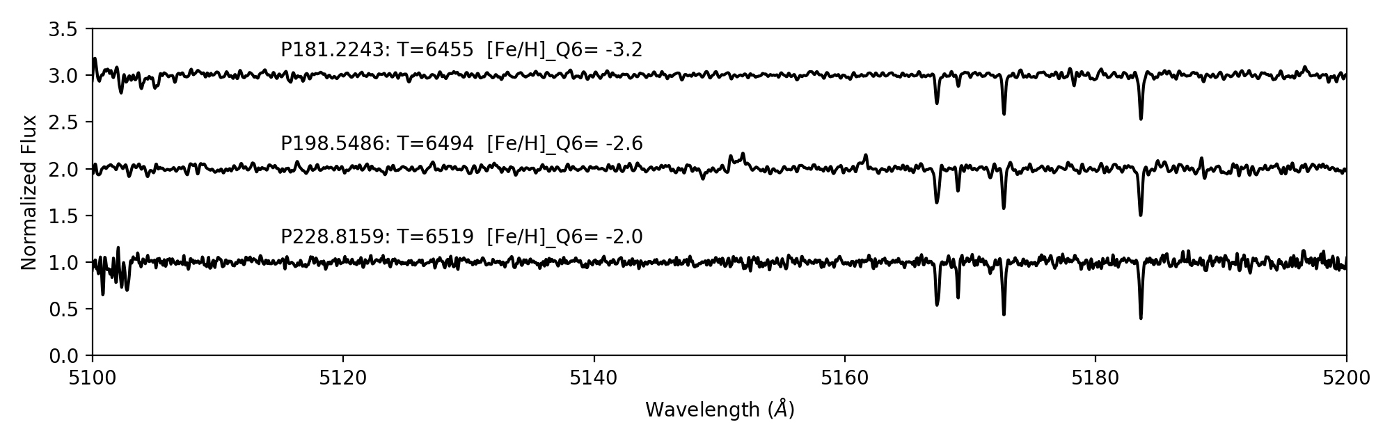
Sample spectra are shown for six targets; three hot (T6500 K), main sequence turn-off stars and three cool (T4900 K) red giants in Fig. 5. These spectra are labelled with their target name, temperature (from the Bayesian inference method, see Section 4.1), and metallicity [Fe/H]Q6 from this "Quick Six" analysis.
Departures from LTE are known to overionize the Fe i atoms due to the impact of the stellar radiation field, particularly in hotter stars and metal-poor giants. These non-LTE (NLTE) effects can be significant in our stellar parameter range, such that NLTE corrections typically reduce the line scatter and improve the Fe i=Fe ii ionization balance (Amarsi et al. 2016; Sitnova et al. 2015; Mashonkina et al. 2019). NLTE effects are explored in this "Quick Six" analysis, by comparing the results from Mashonkina et al. 2017a; Mashonkina et al. 2019 and the INSPECT table77 7 INSPECT non-LTE corrections available at http://inspect-stars.com. (Amarsi et al. 2016; Lind et al. 2012). INSPECT provides data for one of the selected lines, Fe i 5269, where the NLTE correction is (Fe i) , over our parameter space, where Fe i(NLTE) = Fe i(LTE) + (Fe i). Based on a similar treatment for inelastic collisions (of Fe i with H i), Mashonkina et al. 2017a predict similar NLTE corrections for the other three Fe i lines (4957, 5372 and 5397). The largest NLTE corrections ((Fe i) ) are for stars on the subgiant branch, while main sequence stars have zero corrections. Recently, Mashonkina et al. 2019 have examined the impact of quantum mechanical rate coefficients on the inelastic collisions, and find that the NLTE corrections could be even larger (more positive) in the atmospheres of warm metal-poor stars, but smaller (even negative) in cool metal-poor stars and with a wide variation depending on the specific spectral line. This suggests that the NLTE calculations for Fe i need further study; however, given that these corrections in the literature are smaller than or equal to our measurement errors, then we do not apply the NLTE corrections in this "Quick Six" analysis.
The Fe i and Fe ii individual line abundances are averaged together to find [Fe/H]Q6 and the standard deviation [Fe/H]Q6. Each of these results and the total number of lines used (6) are shown in Table 3. From this analysis, we find that several of the Pristine metal-poor candidates are not metal-poor. A comparison of the [Fe/H]Q6 iron abundances to the [Fe/H]Pristine predictions are shown in Fig. 6. These results are similar to the medium resolution spectral analyses (Youakim et al. 2017; Aguado et al. 2019a), and discussed further in Section 4.5.
4.3 Comparing stellar temperatures
A comparison of stellar temperatures from the Bayesian inference method (Section 4.1) to the SDSS colour temperature (TSDSS) is shown in Fig. 7. TSDSS were the initial temperature estimates calculated using the InfraRed Flux Method88 8 IRFM, see https://www.sdss. org/dr12/spectro/sspp_irfm/., assuming [Fe/H] , and based on SDSS (g-i) photometry. An average of the dwarf and giant solutions was used. For 10 stars, their () colours are unreliable because of saturation flags, and we adopt the relation based on the () colours from Ivezić et al. 2008. With this relation, a 200 K offset was applied to move from [Fe/H] to [Fe/H] . Thus, we expect these values of TSDSS to be an oversimplification, and are not surprised by the comparisons in Fig. 7, which are colour-coded by the "Quick Six" metallicities [Fe/H]Q6.
Ignoring the metal-rich stars, then there is still a systematic offset between these methods for the metal-poor stars: the TSDSS colour temperatures are too hot by 150 K for stars between T = K, but they are too cool by 200 K for stars with T K. This offset is similar to the uncertainties in the Bayesian inference method temperatures (TBayes) for most stars, where TBayes ranges from 10 to 200 K (Table 3). The very small colour temperature errors dT10 K in Table 1 are based on the difference between the dwarf/giant solutions, and are not realistic uncertainties.
4.4 Comparing gravity and Fe i=Fe ii
Ionization balance has traditionally been used as an indicator of surface gravity in a classical model atmospheres analyses. Therefore, we compare the log values from the Bayesian inference method (Section 4.1) to the difference in the [Fe i] and [Fe ii] abundances, in Fig. 8. This figure is colour-coded by the "Quick Six" spectroscopic metallicities ([Fe/H]Q6). For the metal-poor stars, the majority of our stars show Fe i=Fe ii to within 2 of the measurement errors, with a mean offset of [Fe i] [Fe ii] . The measurement errors are calculated as the line weighted average of Fe i and Fe ii.
For stars with poor agreement between iron ionization states, the cause cannot be due to neglected NLTE effects which appear to increase the Fe i abundance even further (see in Section 4.2). The offset is primarily seen in the cooler stars in our sample that are on the red giant branch (with lower gravities). For these stars, the NLTE corrections are expected to be small ((Fe i)0.15). For stars closer to the main sequence turn off, the NLTE corrections can be larger; however, the offset between the Fe i and Fe ii abundances seems smaller for those stars in our results. Therefore, the source of ionization equilibrium offsets is not yet clear.
For the metal-rich stars, we expect the surface gravities to be unreliable since the photometric Pristine metallicities [Fe/H]Pristine were assumed a priori in the Bayesian inference method. We do not investigate the metal-rich stars beyond our "Quick Six" analysis.

4.5 Comparisons with medium resolution spectroscopic analyses (FERRE)
A simultaneous Pristine survey program has been carried out for fainter stars (15 V 17) with medium resolution (R ) spectroscopy at the 2.4-m Isaac Newton Telescope (INT), 4.2-m William Herschel Telescope, and 3.6-m New Technology Telescope (Aguado et al. 2019a). These spectra have been observed with uniform spectral wavelength coverage, 360-550 nm, and analysed using the ASSET synthetic spectral grid (Koesterke et al. 2008). Both the observed and the synethetic spectra have been continuum normalized with the same functions, and the minimization algorithm FERRE (Allende Prieto et al. 2006) is applied to derive the stellar parameters (temperature, gravity, metallicity, carbonacity).
The most recent analysis of the medium resolution spectroscopic data includes 946 stars (Aguado et al. 2019a), where 13 of those stars are also in our sample of 70 high probability metal-poor stars (recall, that only 5 were observed at the INT first, and did not affect our target selections). In Figs. 8, 9, and 10, the surface gravities, temperatures, and metallicities are compared between the two analyses for the 13 stars in common. The large differences in gravity are from the systematic errors in the medium resolution FERRE analysis. While the FERRE analysis struggles with precision gravities, both methods are still able to break the dwarf-giant degeneracies sufficiently.

There is a clear relationship between the temperatures such that those determined from isochrones in the Bayesian inference method are cooler by 200 K near 5000 K and hotter by 500 K near 6700 K compared to the FERRE temperatures. These offsets are slightly smaller when compared with the SDSS colour temperatures TSDSS. These temperature differences correlate with small-to-moderate metallicity offsets ([Fe/H]) for stars cooler than 6000 K, whereas two of the hotter stars show larger metallicity offsets, [Fe/H] . In summary, this analysis adopts the stellar parameters from the Bayesian inference method, and finds that the hot stars are hotter and less metal-poor than the results from the medium resolution FERRE analysis.
5 New stars with [Fe/H]


We have identified 28 new metal-poor stars, with spectroscopic metallicity [Fe/H], and where both [Fe i/H] and [Fe ii/H] are below dex (with the exception of Pristine_198.5486+11.4123, with [Fe i/H], which we retain because of its interesting orbit, discussed below). In this section, a more complete LTE, 1D model atmosphere analysis is carried out for a larger set of spectral lines and chemical elements.
As a comparison star, a spectrum of HD 122563 from the CFHT archive was analysed using the same methods as for the Pristine survey targets. Its metallicity is adopted from the literature, i.e., [Fe/H] (see Collet et al. 2018, and references therein), and our methods using its SDSS colours and Gaia DR2 parallax measurements yield stellar parameters that are in good agreement with the literature: Teff = K, log = . Microturbulence () was set to 2.0 km s-1 using the relationship with gravity from Mashonkina et al. 2017a.
For all 28 Pristine survey stars and HD122563, we identify and measure as many clean spectral lines as possible for a detailed abundance analysis, including more lines of Fe i and Fe ii for higher precision iron abundances (than from the [Fe/H]Q6 analysis). Starting with the spectral line list from Norris et al. 2017, spectral features were identified and measured using DAOSpec (Stetson & Pancino 2008), and frequently checked by measuring the area under the continuum using IRAF/. Atomic data were updated when appropriate by comparing to the linemake atomic and molecular line database99 9 linemake contains laboratory atomic data (transition probabilities, hyperfine and isotopic substructures) published by the Wisconsin Atomic Physics and the Old Dominion Molecular Physics groups. These lists and accompanying line list assembly software have been developed by C. Sneden and are curated by V. Placco at https://github.com/vmplacco/linemake.. Abundance results from the model atmospheres analysis are compared to the solar (photospheric) abundances from Asplund et al. 2009.
5.1 Iron-group elements
The 28 new very metal-poor stars were initially identified from their [Fe/H]Q6 abundances in Table 3.
The iron abundances have been recalculated from 2-86 lines of Fe i, 2-6 lines of Fe ii; see Table 5. A 3 minimum equivalent width was used to calculate an upper limit for Fe ii for one star. The line-to-line scatter in the Fe i abundances range from (Fe i) = 0.12 to 0.24, even when only a small number of lines were measured. This is noteworthy because when other elements have lines, we adopt the larger of (X) or (Fe i)/ as a better representation of their line scatter.
These extended iron line measurements and abundances are not used to redetermine the spectroscopic stellar parameters for three reasons: (1) low sensitivity to the precise metallicity in the Bayesian inference method for the confirmed metal-poor stars, (2) insufficient number of lines of Fe ii (and often Fe i) for a fully independent analysis, and (3) the SNR of our CFHT ESPaDOnS spectra () is such that individual measurements of weak lines remain somewhat uncertain. The total iron abundance [Fe/H] is calculated as a weighted mean of Fe i and Fe ii, and the total error [Fe/H] as ([Fe/H])/(NFe i+NFe ii)1/2. These iron abundances are shown in Fig. 11 (top panel), where the errorbars include the systematic errors from the stellar parameter uncertainties added in quadrature (see Section 5.5, though the systematic errors tend to be much smaller).
There is good to fair agreement between Fe i and Fe ii, such that [Fe i] [Fe ii] ranges from to . There is a median offset for the sample, which is not due to NLTE corrections (see the discussion in Section 4.2). This may be due to the lack of Fe ii lines in our metal-poor stars spectra for robust measurements, but another possibility is a systematic gravity uncertainty g. High resolution spectra at bluer wavelengths (4000 Å) would provide more lines of Fe ii to test this in the future. We also examine the slopes in the Fe i line abundances vs excitation potential (, in eV) to test our temperature estimates. A meaningful slope could be measured when N(Fe i) and eV, and all slopes were found to be relatively flat, dex/eV. This gives us more confidence in the fidelity of the temperatures TBayes, and thereby the Bayesian inference method for calculating stellar parameters and uncertainties.
The other iron-group elements (Cr and Ni, listed in Table 5) are in good agreement with [Fe/H], and/or other Galactic halo stars at similar metallicities; see Fig. 11. Cr is determined from 1-3 lines of Cr i (5206.0, 5208.4 , and 5409.8 Å); only the spectrum of Pristine_245.8356+13.8777 had sufficient SNR at blue wavelengths that the lines at 4254.3, 4274.8, and 4289.7 Å could also be observed. [Cr/Fe] is subsolar in metal-poor stars, suggested as a NLTE effect (Bergemann & Cescutti 2010). Ni is determined from 1-2 lines of Ni i (5035.4, 5476.9 Å). Three additional lines were available in the high SNR spectrum of HD 122563 (5080.5, 6643.6, and 6767.8 Å). The [Ni/Fe] results are within of the solar ratio, similar to other Galactic halo stars.
The -element abundances (Mg and Ca) in the 28 new very metal-poor stars are listed in Table 6. Upper limits are determined for some stars by computing 3 minimum equivalent widths. The -elements form through hydrostatic H- and He-core burning stages, though some Ca can also form later during SN Ia events. Because of these different nucleosynthetic sites, the [Mg/Ca] ratio need not scale together at all metallicities, as seen in some dwarf galaxies such as the Carina and Sextans dwarf galaxies (Norris et al. 2017; Jablonka et al. 2015; Venn et al. 2012, e.g., ), also the unusual star cluster NGC 2419 (Cohen & Kirby 2012). We also include our discussion of Ti in this section even though it does not form with the -elements. The dominant isotope 48Ti forms primarily through Si-burning in massive stars (Woosley et al. 2002, e.g.,), and yet it seems to scale with other -elements in metal-poor stars in the Galaxy.
Mg is determined from 2-3 lines (5172.7, 5183.6, 5528.4 Å), and a fourth line (4703.0 Å) was measurable in one star (Pristine_245.8356+13.8777). In Fig. 12, a larger scatter can be seen in the [Mg/Fe] results, though this is similar to the Galactic comparison stars. One star shows sub-solar [Mg/Fe] by more than (Pristine_251.4082+12.3657). Another star has high [Mg/Fe], validated from all three Mg i lines (Pristine_181.2243+07.4160), also shown in Fig 13.
5.2 -elements
The calcium abundances are determined from 1-9 lines of Ca i. The [Ca/Fe] abundances are in good agreement with each other, and with the Galactic comparison stars, as seen in Fig. 12. The same star with low [Mg/Fe] (Pristine_251.4082+12.3657) also has a very low [Ca/Fe] upper limit. This star is discussed further in Section 6.2.
Titanium has been determined from 1-9 lines of Ti i and 2-11 lines of Ti ii. When both are unavailable, upper limits are determined from two Ti ii lines (which provide stronger constraints than the Ti i features). In Fig. 12, the unweighted average results of [Ti i/Fe] and [Ti ii/Fe] are shown.
NLTE corrections have not been incorporated for Mg, Ca, or Ti because they tend to be small to negligible ( dex) according to the INSPECT database (for Mg i) and Mashonkina et al. 2017b. For Ti i, three lines (4981.7, 4991.1, 4999.5 Å) are available in the INSPECT database, which suggests large corrections dex. However NLTE corrections for the same lines from Sitnova et al. 2016, using a model atom that includes important high excitation levels of Ti i, are significantly smaller, dex. NLTE corrections should be included, but most of our stars have Ti i Ti ii to within 1 (our measurement errors) in LTE. Therefore, for this analysis, where the maximum SNR per star is , we do not include the small NLTE corrections, and note that the good agreement with the Galactic comparison stars and Ti ionization balance furthers our confidence in the stellar parameters from the Bayesian inference method.
No oxygen abundances or upper limits were determined since the [OI] 6300 and 6363 Å lines are weak and in a region that is poorly cleaned of telluric contaminants.
5.3 Odd elements
Odd elements, Na and Sc, are listed in Table 6. These have different nucleosynthetic sources and are not related to one another. We also include a comment on Li upper limits at the end of this section.
In metal-poor stars, sodium typically forms with the -elements during core collapse SN. On the other hand, scandium forms in the iron core of a massive star with a yield that strongly depends on the proton-to-neutron ratio (Ye), and it is very sensitive to neutrino processes (Woosley et al. 2002; Curtis et al. 2019, e.g.,).
Sodium abundances are initially from the LTE analysis of the Na i D lines (5889.9, 5895.9 Å), which unfortunately can be strong, therefore sensitive to microturbulence in a 1D LTE analysis, and also contaminated by interstellar Na. Furthermore, since they originate from the Na i ground state, they are subject to NLTE effects. NLTE corrections are similar between the INSPECT database and Mashonkina et al. 2017c; [Na/H][Na/H]Na, where Na = to dex. The Na i subordinate line (5688.2 Å) could only be used for upper limit estimates at the SNR of our spectra.
Despite the large NLTE corrections, four stars were found with initially very high Na i abundances (Pristine_251.4082+12.3657, Pristine_193.8390+11.4150, Pristine_217.5786+14.0379, and Pristine_250.6963+08.3743, in order of decreasing metallicity). These four stars also have the lowest radial velocities in our sample (-5, +4, -16, and -4 km s-1, in order of decreasing metallicity), and we suggest they are contaminated by the interstellar Na lines. To test this, their Na i D line shapes were compared with other spectral lines in the same stars and found to be slightly broader (occassionally, the line core is even split); their Na i D line shapes are also broader than similar stars with higher radial velocities (where the interstellar lines are often seen offset from the stellar lines). Thus, in Fig. 14, the highest Na abundances are noted as upper limits only since they are most likely blended, and for the other stars the NLTE corrected Na abundances are shown.
Sc ii has been measured from 1-3 lines (5031.0, 5526.8, 5657.9 Å) in five metal-poor Pristine stars, and the comparison star HD 122563, and upper limits were determined in the others. With an odd number of nucleons, this species undergoes strong hyperfine splitting, which affects line formation through de-saturation. The HFS corrections were found to be small (). Upper limits have also been determined for Sc ii in most of the other new metal-poor stars. Upper limits were examined for Mn i as well, but did not provide interesting constraints.
Lastly, we mention Li in this section. Estimates from the Li i 6707 Å line provide upper limits that do not provide meaningful constraints, i.e., the upper limits are above the standard Big Bang nucleosynthesis value of A(Li) = 2.7 (Spergel et al. 2003, e.g., from WMAP,). Only two stars (Pristine_229.1219+00.9089 and Pristine_237.8246+10.1426) have 3 equivalent width (35 mÅ) upper limits of A(Li) , which is similar to most metal-poor stars that lie on (or below) the Spite Plateau (Aguado et al. 2019b; Bonifacio et al. 2018, e.g., see).
5.4 Heavy elements
Abundances for the neutron-capture elements Y and Ba in the 28 new very metal-poor stars are listed in Table 5. Up to four lines of Ba ii (4554.0, 5853.7, 6141.7, and 6496.9 Å) and two lines of Y ii (4883.7, 4990.1 Å) could be measured. Unfortunately no lines or useful upper limits for Eu are available in our CFHT spectra. When no lines were observable, we determined upper limits from 3 minimum equivalent width estimates. Hyperfine splitting and the isotopic splitting has been included in the Ba analysis. Most stars have [Ba/Fe] in good agreement with the Galactic comparison stars.
All six lines were measured in only one star near [Fe/H] (Pristine_214.5555+07.4670). This star is enriched in both Y and Ba, and we identify it as an r-process rich star. Without Eu, it cannot be further classified as r-I or r-II (Christlieb et al. 2004; Sakari et al. 2018b). Studies of r-process rich stars have found a nearly identical main r-process pattern (from barium, A=56, to hafnium, A=72) in all types of stars, in all environments, and with variations only between the lightest and heaviest elements (see Roederer et al. 2010; Hill et al. 2017; Sakari et al. 2018a, and references therein). No other elements stand out in this star; however, as one of the hotter turn-off stars in our sample, there are not many other features or elements to analyse at the SNR of our spectra.
Two more stars show [Ba/Fe]+0.5 (Pristine_237.8246 +10.1426, Pristine_210.0166+14.6289). These lie above the typical [Ba/Fe] values found in the Galactic halo metal-poor stars by Roederer et al. 2014, and their results are securely derived from 2 - 4 Ba ii line measurements. However, no Y ii lines were observed in either (and the Y ii upper limits do not provide useful constraints). The two may be moderately r-process enriched stars.
Possibly of greater interest are the two most Ba-poor stars (Pristine_181.4395+01.6294 and Pristine_193.8390+11.4150). Low Ba is very unusual at their metallicities when compared with the other Galactic halo stars, as seen in Fig. 15. This composition is similar to stars in the Segue 1 and Hercules ultra faint dwarf (UFD) galaxies (Frebel et al. 2014; Koch et al. 2013). In Segue 1, the Ba-poor stars were discussed as representative of inhomogeneous enrichment by a single (or few) supernova events, and therefore possibly related to first stars. Higher SNR data for these two stars is warranted in order to test this hypothesis.
Finally, one star (Pristine_245.8356+13.8777) shows a high Y ii abundance, but normal Ba ii abundance. A similar star was recently studied by Caffau et al. 2019, where the authors show it is a CEMP-s star, having undergone mass transfer in a binary system with an Asymptotic Giant Branch (AGB) star. However, they also suggest that the AGB star in this system may have undergone a proton ingestion event just before the mass transfer that produced an enhancement in only the first s-process peak elements.

5.5 Abundance uncertainties
Total uncertainties in the chemical abundances are a combination of the measurement uncertainties and systematic errors in the stellar parameters, added in quadrature. For the measurement errors, when fewer than 4 lines are available for an element X, then we adopt the larger of (X) or (Fe i)/sqrt(NX). Since Fe i lines are measured across the entire spectrum and over a range of equivalent widths and excitation potentials, then this assumes that (Fe i) captures the minimum measurement quality of our spectra. For the systematic errors, due to uncertainties in the stellar parameters, we determine the impact of the changes in temperature, gravity, and metallicity listed in Table 3.
A sample of the systematic uncertainties for three stars that cover the parameter space of this sample are shown in Table 8. It can be seen that temperature tends to be the dominant systematic error in the analysis of most elements. While we could further investigate the impact of the final metallicities [Fe/H] and uncertainties ([Fe/H]) through iterations in the Bayesian inference method on the model atmospheres parameters, we did not; the only stars that we follow up in detail are those that did prove to be very metal-poor, therefore the impact of adjusting for the final metallicities on the other stellar parameters is very small.

6 Discussion
A total of 70 (out of 115) bright, metal-poor candidates have been observed with the CFHT ESPaDOnS spectrograph from the original footprint (1000 sq deg) of the Pristine survey. These targets were selected to have a high probabilily for [Fe/H], when the Pristine CaHK filter was calibrated with the SDSS g-i and g-r colours (60 stars), or only the SDSS g-r colour alone (10 stars). We carry out a model atmospheres analysis by adopting stellar parameters determined from a Bayesian inference method that uses the SDSS colours, Gaia DR2 parallaxes, and MESA/MIST isochrones, assuming the initial Pristine survey metallicities. Out of these 70 selected stars, we have found 28 to indeed have low metallicities, [Fe/H] (40%). The Pristine survey had also predicted 27 stars would have [Fe/H], and 5 were found (19%). Of the 42 remaining stars ( [Fe/H]), there are no obvious relationships with any other stellar parameters (e.g., see Fig. 16), although we notice that all of the candidates on the upper red giant branch were successfully selected and confirmed to be metal-poor stars.
The selections made in this paper differ from those used by Youakim et al. 2017 and Aguado et al. 2019a, see Section 2, being far more strict in the metal-poor probability cuts. Furthermore, about 1/3 of the targets in this program were observed before the selection criteria were finalized. Nevertheless, our success rates are very similar to the results from the medium resolution surveys. We do not reproduce the (lower) success rates for bright stars seen in earlier Pristine survey papers (Caffau et al. 2017; Bonifacio et al. 2019), partially due to our improved (more strict) selection criteria, partially due to differences between the SDSS and APASS photometry, and possibly due to the larger number of stars in this sample.
In the remainder of this Discussion, we examine the kinematic and orbital properties of the 70 metal-poor candidates in this paper, and correlate those with their chemical abundances. We caution that these calculations and our interpretations are highly dependent on the accuracy of the adopted Milky Way potential (described in the next section). For example, our orbit integrations do not account for effects like the Galactic bar, which can significantly influence halo star orbits (Price-Whelan et al. 2016; Hattori et al. 2016; Pearson et al. 2017, e.g.,).
6.1 Kinematics and Orbits
Galactocentric velocities (U, V, W) are calculated for each star from their Galactic Cartesian coordinates (X,Y,Z) following the methods of Bird et al. 2019. The distance between the Sun and the Galactic centre is taken to be 8.0 kpc, the Local Standard of Rest circular velocity is Vcirc = 239 km s-1, and the peculiar motion of the Sun is (U0 = 11.10 km s-1; V Vcirc = 251.24 km s-1; W0 = 7.25 km s-1, as described in Schönrich et al. 2010. The sign of U0 is changed so that U is positive towards the Galactic anticentre. Errors in these velocities are propagated from the uncertainties in proper motion, radial velocities, and distance by calculating the mean dispersions from 1000 Monte-Carlo realisations, and selecting from a Gaussian distribution in each of the original quantities.

With the distances from the Bayesian inference analysis1010 10 For three stars, we reverted back to distances from their 1/parallax values based on unrealistical outer halo distances and other orbital properties. Two of these stars were discussed at the end of Section 4.1, and a third star is discussed in Appendix A., precision radial velocities from our high resolution spectra, and proper motions from the Gaia DR2 database, then the orbital parameters for the sample are calculated using the Galpy package (Bovy 2015). The MWPotential14 is adopted, a Milky Way gravitational potential composed of a power-law, exponentially cutoff bulge, Miyamoto Nagai Potential disk, and Navarro et al. 1997 dark matter halo. A more massive halo is chosen following Sestito et al. 2019, with a mass of of 1.2 x 10¹² M⊙ which is more compatible with the value from Bland-Hawthorn & Gerhard 2016.
The UVW velocities for the 70 highly probable metal-poor stars in this sample are given in Table 9. The Toomre diagram for these objects are shown in Fig. 17, colour-coded by the [Fe/H]Q6 metallicities. Most of the metal-poor stars in our sample have halo-like velocities, as expected for their metallicities. One very metal-poor star (Pristine_183.6849+04.8619, discussed below) appears to have disk-like dynamics.
6.2 Orbit Analyses
To investigate the relationships between the chemical and kinematic properties of the stars in our sample, we examine their maximum excursions. This includes the apocentric and pericentric distances (Rapo and Rperi), perpendicular distance from the Galactic plane (Zmax), and eccentricity (e) of the derived orbits; see Table 9.

In Fig. 18, stars with R kpc and Z kpc are considered to be confined to the Galactic plane (16 stars), while stars with R kpc are considered to be members of the outer halo (10 stars). The outer halo star Pristine_251.4082+12.3657 has the largest distance in our sample, with a highly eccentric orbit, and it is one of the most metal poor stars ([Fe/H]=), with low abundances of [Mg/Fe] and [Ca/Fe] (see Fig. 12), and also low [Ba/Fe]. This chemical signature is typical of stars in or accreted from the nearby dwarf galaxies. Alternatively, it may have been accreted from an ultra faint dwarf galaxy, since its chemistry is also similar to the unique stars CS 29498-043 and CS 29249-037 (Aoki et al. 2002; Depagne et al. 2002), both near [Fe/H]. These stars have been proposed to be second-generation stars, that formed from gas enriched by a massive Population III first star, exploding as a fall-back supernova (Frebel et al. 2019, see also), and as such they would have formed in a now accreted ultra faint dwarf galaxy.
In Fig. 19, only stars with R kpc are shown. Clearly, most of the stars confined to the Galactic plane (Z kpc) are the relatively metal-rich (interloping) stars in our sample. However, one of the most metal-poor stars (Pristine_183.6849+04.8619, [Fe/H] ) is also confined to the Galactic plane with a nearly circular orbit (e=0.3). This was also seen in the Toomre diagram (Fig. 17). A detailed view of the orbit of this star is shown in Fig. 20. Most of the spectral lines in this star are weak and so we were unable to determine many elemental abundances, only [Mg/Fe]=+0.13 (0.14) and [Na/Fe]= (), which are both quite low for a typical halo metal-poor star. Ultra metal-poor stars ([Fe/H]) have been found on similar quasi-circular and planar orbits by Sestito et al. 2019, and interpreted as stars that may have been brought in during the early merger phase of the building blocks of the proto-MW that eventually formed the disk.
Several (8) stars in our sample have orbits that take them deep into the Galactic bulge (R kpc). All of these stars are on highly radial orbits (e ), and two are very metal-poor; Pristine_250.6963+08.3743 at [Fe/H], and Pristine_201.8710+07.1810 at [Fe/H]. While the former star shows typical halo abundances in [(Mg,Ca,Ti)/Fe] (0.4), the latter is clearly challenged in -elements, [(Na,Mg)/Fe] (0.2). It is difficult to discern whether these stars formed in the bulge and have been flung out or if they have been accreted from the halo (or a dwarf galaxy) and moved inwards. As metal-poor stars in the bulge are thought to be older in absolute age (Tumlinson 2010; Howes et al. 2016; Starkenburg et al. 2017a; El-Badry et al. 2018; Frebel et al. 2019), then these could be extremely valuable objects for studies of the earliest stages of star formation in the Galaxy.
6.3 Action Parameters
The orbital energy (E) and action parameters (vertical Jz, azimuthal Jϕ) were determined during the Galpy orbit calculations (discussed above); these are shown in Fig. 21 and provided in Table 9. Values are scaled by the solar values, where Jϕ⊙ = 2009.92 km s-1 kpc, Jz⊙ = 0.35 km s-1 kpc and E⊙ = -64943.61 (km s-1)2. It is worth noting that stars with Jϕ/Jϕ⊙ = 1 rotate like the Sun around the Galactic Centre.

Amongst the very metal-poor stars, we note they are roughly evenly distributed between retrograde and prograde orbits, i.e., between Jϕ/J. The most retrograde metal-poor star with a bound orbit (near Jϕ/J) is Pristine_198.5486+11.4123. This star has Z kpc, placing it very close to the Galactic plane. Therefore, this star is travelling at nearly the speed of the Sun but in the opposite direction, close to the Galactic plane. This orbit is certainly unusual and suggests it may have been accreted from a dwarf galaxy; however, its chemistry is like that of a normal metal-poor star, [Fe/H], [Mg/Fe]=+0.3, and [Ba/Fe]+0.4.
The very metal-poor star Pristine_251.4082+12.3657, identified as having the largest value in this sample is also found to have a large Jz/Jz⊙ value and an unbound orbit (E/E). In total, three stars in Fig. 21 appear to have unbound orbits, although we caution that our uncertainties in their orbits are quite small when based on the very small distance errors from the Bayesian inference method. Examination of their parallax errors show that their orbits could be bound, consistent with E/E. In Appendix A, we examine five more stars that appear to be dynamically unbound when their Bayesian inferred distances are used to determine their orbits. Two of those stars were discussed in Section 4.1, and it was shown that the orbital properties for these two metal-rich stars were significantly improved when 1/parallax was adopted for their distances. The same was found for a third star Pristine_213.7879+08.4232, even though this star has been confirmed to be metal-poor. The parallax errors for these three stars are all very small, and therefore we have adopted the 1/parallax distance for the orbital analysis of these three stars. Finally, we removed two stars from this kinematic analysis, Pristine_181.4395+01.6294 and Pristine_182.5364+00.9431. Both stars have R500 kpc and e1 resulting in extreme and unbound orbits for any distance that we adopt.
One of the most exciting discoveries from the Gaia DR2 dataset has been the identification of the Gaia-Enceladus dwarf galaxy (or galaxies) dissolved into the Milky Way halo. The region where stars may be associated with Gaia-Enceladus is shown in Fig. 21, i.e., E/E and Jϕ/J (Helmi et al. 2018; Haywood et al. 2018; Belokurov et al. 2018; Myeong et al. 2018; Myeong et al. 2019). This includes eight stars in our sample that range from [Fe/H], with a mean metallicity of [Fe/H]=; see Table . Only one of these stars is sufficiently metal-poor to have made it into our detailed analysis sample, Pristine_250.6963+08.3743 ([Fe/H]=). This star has high -element abundances [(Ca,Ti)/Fe], but lower magnesium such that [Mg/(Ca,Ti)]=, which is has been seen in some dwarf galaxies (e.g., Tri II, Venn et al. 2017). However, unlike most stars in dwarf galaxies, this star appears to have solar-like [Ba/Fe] and [Sc/Fe]. It is unclear if this star is a true member of the original Gaia-Enceladus accretion event, but if so it would be amongst the most metal-poor stars yet found in that system (though also see Monty et al. 2019). As a final test, we examine the action-energy space of the newly discovered Gaia-Sequoia accretion event (Myeong et al. 2018; Myeong et al. 2019), i.e., E/E and Jϕ/J, but find no targets in that parameter space.
7 Conclusions and Future Work
The results from our follow-up spectroscopy of 115 bright metal-poor candidates selected from the Pristine survey has been presented based on CFHT ESPaDOnS spectra. We have discovered 28 new very metal-poor stars with [Fe/H] and five stars with [Fe/H], which imply success rates of 40% (28/70) and 19% (5/27), respectively. These rates are higher than previous surveys, though in line with the Pristine medium resolution programs. A detailed model atmospheres analysis for the 28 new very metal-poor stars, has provided stellar parameters and chemical abundances for 10 elements (Na, Mg, Ca, Sc, Ti, Cr, Fe, Ni, Y, Ba) and Li upper limits. Most stars show chemical abundance patterns that are similar to the normal metal-poor stars in the Galactic halo; however, we also report the discoveries of a new r-process rich star (Pristine_214.5556+07.4670), a new CEMP-s candidate with [Y/Ba] (Pristine_245.8356+13.8777), and a [Mg/Fe] challenged star (Pristine_251.4082+12.3657) which has an abundance pattern typical of stars in dwarf galaxies or, alternatively, gas enriched by a massive Population III first star exploding as a fall-back supernova. Two stars are also interesting because they are quite Ba-poor (Pristine_181.4395+01.6294 and Pristine_193.8390+11.4150), and resemble stars in the Segue 1 and Hercules UFDs, which have been interpreted as evidence for inhomogeneous enrichment by a single (or few) supernovae events, and therefore possibly related to first stars.
The kinematics and orbits for all 70 of the metal-poor candidates have been determined using Gaia DR2 data, our radial velocities, and adopting the MWPotential14 in the Galpy package (with a slightly more massive halo). The majority of the confirmed metal-poor stars are members of the Galactic halo, although some stars show unusual kinematics for their chemistry. We report the discovery of a very metal-poor ([Fe/H] ) star (Pristine_183.6849+04.8619) with a slightly eccentric () prograde orbit confined to the Galactic plane (Z kpc). We also find a metal-poor ([Fe/H] ) star (Pristine_198.5486+11.4123) on a highly retrograde orbit (V km s-1, Jϕ/J) that remains close to the Galactic plane (Z kpc). These two stars do not fit standard models for the formation of the Galactic plane, pointing towards more complex origins. An additional eight stars were found to have orbital energy and actions consistent with the Gaia-Enceladus accretion event, including one very metal-poor star (Pristine_ 250.6963+08.3743) with [Fe/H]= and chemical abundances that are common for stars in dwarf galaxies. Finally, eight stars have highly radial orbits that take them deep into the Galactic bulge (R kpc), including two very metal-poor stars (Pristine_250.6963+08.3743 at [Fe/H], and Pristine_201.8710+07.1810 at [Fe/H], the latter star is also low in -elements). If these stars formed in the bulge, they could be extremely valuable for studies of the earliest conditions for star formation in the Galaxy.
Currently, we are running a Gemini/GRACES Large and Long Program to follow-up with high SNR () spectra for our best metal-poor candidates ([Fe/H] ) and with V selected from medium resolution spectroscopy. We also plan to observe a selection of these stars with the upcoming Gemini GHOST spectrograph (Chene et al. 2014; Sheinis et al. 2017), which is anticipated to have excellent throughput at blue-UV wavelengths, providing far more iron-group lines for stellar parameter assessments and many more spectral lines of heavy neutron-capture (and light) elements.
In the near future, massively multiplexed high resolution spectroscopic surveys (R ) will be initiated, including the European WEAVE survey at the Isaac Newton Telescopes (Dalton et al. 2012), the 4MOST survey at ESO (De Jong et al. 2019), and the SDSS-V survey comprising fields in both the northern and southern hemispheres (Kollmeier et al. 2017). These will provide the truly large statistical samples needed for studies of the metal-poor Galaxy.
Acknowledgements
This work is based on observations obtained at the Canada-France-Hawaii Telescope (CFHT) which is operated by the National Research Council of Canada, the Institut National des Sciences de l’Univers of the Centre National de la Recherche Scientique of France, and the University of Hawaii. This work has made use of data from the European Space Agency (ESA) mission Gaia (https://www.cosmos.esa.int/gaia), processed by the Gaia Data Processing and Analysis Consortium (DPAC, https://www.cosmos.esa.int/web/gaia/dpac/consortium). Funding for the DPAC has been provided by national institutions, in particular the institutions participating in the Gaia Multilateral Agreement. This research has made use of use of the SIMBAD database, operated at CDS, Strasbourg, France (Wenger et al. 2000). The authors wish to thank David Yong and Ian Roederer for help discussions on the detailed abundances of the new metal-poor stars.
This work was funded in part through the National Science and Engineering Research Council Discovery Grants program and the CREATE training program on New Technologies for Canadian Observatories. The authors thank the International Space Science Institute, Berne, Switzerland, for providing financial support and meeting facilities to the international team Pristine. FS and NFM gratefully acknowledge funding from CNRS/INSU through the Programme National Galaxies et Cosmologie and through the CNRS grant PICS07708. FS thanks the Initiative dExcellence IdEx from the University of Strasbourg and the Programme Doctoral International PDI for funding his PhD. This work has been published under the framework of the IdEx Unistra and benefits from funding from the state managed by the French National Research Agency (ANR) as part of the investments for the future program. JIGH acknowledges financial support from the Spanish Ministry of Science, Innovation and Universities (MICIU) under the 2013 Ramón y Cajal program MICIU RYC-2013-14875, and also from the Spanish ministry project MICIU AYA2017-86389-P.
The authors wish to recognize and acknowledge the very significant cultural role and reverence that the summit of Maunakea has always had within the indigenous Hawaiian community. We are most fortunate to have the opportunity to conduct observations from this mountain.
8 Appendix A

Five stars were identified for a more careful dynamical analysis in Section 6.1. When their distances were determined from the Bayesian inference method, these stars had highly energetic and unbound orbits (E/E), with R kpc. These five stars are shown in Fig. 22.
As two of these stars (Pristine_200.5298+08.9768 and Pristine_187.9785+08.7294) were found to have higher metallicities than had been adopted for the MIST stellar isochrone in the Bayesian inference method, then we assumed their Bayesian inferred distances were unreliable. Adopting their distances as 1/parallax from the Gaia DR2 database, then we found sensible orbits and dynamical parameters for both stars. Furthermore, the parallax errors were small for both stars.
We found that the orbit solution for a third star (Pristine_213.7879+08.4232) was also significantly improved by rejecting the Bayesian inferred distance in favour of the 1/parallax value. Again, the parallax error is small, and the resulting orbital properties are less peculiar. It is not clear why the Bayesian method did not work for this star, however we note that this was a target that we observed very early on and it is no longer in the Pristine survey catalogue. Investigating this star a bit further, we notice that the 1/parallax distance is closer than the Bayesian inferred distance, suggesting that the surface gravity for this star may be slightly higher (log = 2.3, may be closer to log 3). In that case, we find small corrections to the abundances, such that log(Fe ii)+0.3, bringing Fe ii into much better agreement with Fe i. The impact on [Fe/H] for this star is negligible though since the iron abundance is dominated by the more numerous spectral lines of Fe i. Minor adjustments to the other elements would have no signficant effect on the chemical analysis and interpretation of this star.
Finally, when examining the impact of the distances for the two stars Pristine_182.5364 ([Fe/H]=) and Pristine_181.4395 ([Fe/H]=), we find they always result in highly retrograde and unbound orbits. The orbit for the more metal-poor of these two stars is highly uncertain when determined from its parallax (/). Interestingly though, this star is also one of the [Ba/Fe]-poor stars discussed in Section 5.4 as possibly accreted from an ultra faint dwarf galaxy. As a sanity check, we also calculated the orbits for all of the other metal-poor candidates in this analysis, but found only small offsets in their orbit and action parameters.
References
- Abadi et al. (2010) Abadi M. G., Navarro J. F., Fardal M., Babul A., Steinmetz M., 2010, MNRAS, 407, 435
- Abel et al. (2002) Abel T., Bryan G. L., Norman M. L., 2002, Science, 295, 93
- Aguado et al. (2019a) Aguado D., Youakim K., et al., 2019a, MNRAS
- Aguado et al. (2019b) Aguado D. S., González Hernández J. I., Allende Prieto C., Rebolo R., 2019b, ApJ, 874, L21
- Allende Prieto et al. (2006) Allende Prieto C., Beers T. C., Wilhelm R., Newberg H. J., Rockosi C. M., Yanny B., Lee Y. S., 2006, ApJ, 636, 804
- Amarsi et al. (2016) Amarsi A. M., Lind K., Asplund M., Barklem P. S., Collet R., 2016, MNRAS, 463, 1518
- Aoki et al. (2002) Aoki W., Norris J. E., Ryan S. G., Beers T. C., Ando H., 2002, ApJ, 576, L141
- Arentsen et al. (2019) Arentsen A., Starkenburg E., Shetrone M. D., Venn K. A., Depagne É., McConnachie A. W., 2019, A&A, 621, A108
- Asplund et al. (2009) Asplund M., Grevesse N., Sauval A. J., Scott P., 2009, ARA&A, 47, 481
- Bailer-Jones et al. (2018) Bailer-Jones C. A. L., Rybizki J., Fouesneau M., Mantelet G., Andrae R., 2018, AJ, 156, 58
- Barbá et al. (2019) Barbá R. H., Minniti D., Geisler D., Alonso-García J., Hempel M., Monachesi A., Arias J. I., Gómez F. A., 2019, ApJ, 870, L24
- Beers & Christlieb (2005) Beers T. C., Christlieb N., 2005, ARA&A, 43, 531
- Beers et al. (1992) Beers T. C., Preston G. W., Shectman S. A., 1992, AJ, 103, 1987
- Belokurov et al. (2018) Belokurov V., Erkal D., Evans N. W., Koposov S. E., Deason A. J., 2018, MNRAS, 478, 611
- Bergemann & Cescutti (2010) Bergemann M., Cescutti G., 2010, Astronomy and Astrophysics, 522, A9
- Bird et al. (2019) Bird S. A., Xue X.-X., Liu C., Shen J., Flynn C., Yang C., 2019, The Astronomical Journal, 157, 104
- Blackwell et al. (1979) Blackwell D. E., Petford A. D., Shallis M. J., 1979, MNRAS, 186, 657
- Bland-Hawthorn & Gerhard (2016) Bland-Hawthorn J., Gerhard O., 2016, ARA&A, 54, 529
- Bonifacio et al. (2018) Bonifacio P., et al., 2018, A&A, 612, A65
- Bonifacio et al. (2019) Bonifacio P., et al., 2019, MNRAS, 487, 3797
- Bovy (2015) Bovy J., 2015, ApJS, 216, 29
- Bromm (2013) Bromm V., 2013, Reports on Progress in Physics, 76, 112901
- Caffau et al. (2012) Caffau E., et al., 2012, A&A, 542, A51
- Caffau et al. (2017) Caffau E., et al., 2017, Astronomische Nachrichten, 338, 686
- Caffau et al. (2019) Caffau E., et al., 2019, A&A, 628, A46
- Casagrande et al. (2016) Casagrande L., et al., 2016, MNRAS, 455, 987
- Chene et al. (2014) Chene A.-N., et al., 2014, in Proc. SPIE. p. 915147 (arXiv:1409.7448), doi:10.1117/12.2057417
- Choi et al. (2016) Choi J., Dotter A., Conroy C., Cantiello M., Paxton B., Johnson B. D., 2016, ApJ, 823, 102
- Christlieb et al. (2002) Christlieb N., et al., 2002, Nature, 419, 904
- Christlieb et al. (2004) Christlieb N., et al., 2004, Astronomy and Astrophysics, 428, 1027
- Christlieb et al. (2008) Christlieb N., Schörck T., Frebel A., Beers T. C., Wisotzki L., Reimers D., 2008, A&A, 484, 721
- Clark et al. (2011) Clark P. C., Glover S. C. O., Smith R. J., Greif T. H., Klessen R. S., Bromm V., 2011, Science, 331, 1040
- Cohen & Kirby (2012) Cohen J. G., Kirby E. N., 2012, ApJ, 760, 86
- Collet et al. (2018) Collet R., Nordlund Å., Asplund M., Hayek W., Trampedach R., 2018, MNRAS, 475, 3369
- Cui et al. (2012) Cui X.-Q., et al., 2012, Research in Astronomy and Astrophysics, 12, 1197
- Curtis et al. (2019) Curtis S., Ebinger K., Fröhlich C., Hempel M., Perego A., Liebendörfer M., Thielemann F.-K., 2019, ApJ, 870, 2
- DaCosta et al. (2019) DaCosta G. S., et al., 2019, Monthly Notices of the Royal Astronomical Society, 489, 5900
- Dalton et al. (2012) Dalton G., et al., 2012, in Ground-based and Airborne Instrumentation for Astronomy IV. p. 84460P, doi:10.1117/12.925950
- Dawson et al. (2013) Dawson K. S., et al., 2013, AJ, 145, 10
- De Jong et al. (2019) De Jong R. S., Others A., Others B., 4MOST team 2019, The Messenger, 175, 3
- Depagne et al. (2002) Depagne E., et al., 2002, A&A, 390, 187
- Donati et al. (1997) Donati J. F., Semel M., Carter B. D., Rees D. E., Collier Cameron A., 1997, MNRAS, 291, 658
- Donati et al. (2006) Donati J. F., Catala C., Landstreet J. D., Petit P., 2006, in Casini R., Lites B. W., eds, Astronomical Society of the Pacific Conference Series Vol. 358, Solar Polarization 4. p. 362
- Dotter (2016) Dotter A., 2016, ApJS, 222, 8
- Eisenstein et al. (2011) Eisenstein D. J., et al., 2011, AJ, 142, 72
- El-Badry et al. (2018) El-Badry K., et al., 2018, Monthly Notices of the Royal Astronomical Society, 480, 652
- Frebel & Norris (2015) Frebel A., Norris J. E., 2015, ARA&A, 53, 631
- Frebel et al. (2006) Frebel A., et al., 2006, ApJ, 652, 1585
- Frebel et al. (2014) Frebel A., Simon J. D., Kirby E. N., 2014, ApJ, 786, 74
- Frebel et al. (2019) Frebel A., Ji A. P., Ezzeddine R., Hansen T. T., Chiti A., Thompson I. B., Merle T., 2019, ApJ, 871, 146
- Freeman & Bland-Hawthorn (2002) Freeman K., Bland-Hawthorn J., 2002, ARA&A, 40, 487
- Gaia Collaboration et al. (2018) Gaia Collaboration Brown A. G. A., Vallenari A., Prusti T., de Bruijne J. H. J., Babusiaux C., Bailer-Jones C. A. L., 2018, preprint, (arXiv:1804.09365)
- Gianninas et al. (2015) Gianninas A., Curd B., Thorstensen J. R., Kilic M., Bergeron P., Andrews J. J., Canton P., Agüeros M. A., 2015, MNRAS, 449, 3966
- González Hernández & Bonifacio (2009) González Hernández J. I., Bonifacio P., 2009, A&A, 497, 497
- Greif (2015) Greif T. H., 2015, Computational Astrophysics and Cosmology, 2, 3
- Gustafsson et al. (2008) Gustafsson B., Edvardsson B., Eriksson K., Jørgensen U. G., Nordlund Å., Plez B., 2008, A&A, 486, 951
- Hartwig et al. (2018) Hartwig T., et al., 2018, MNRAS, 478, 1795
- Hattori et al. (2016) Hattori K., Erkal D., Sanders J. L., 2016, MNRAS, 460, 497
- Hayes et al. (2018) Hayes C. R., et al., 2018, ApJ, 852, 49
- Haywood et al. (2018) Haywood M., Di Matteo P., Lehnert M. D., Snaith O., Khoperskov S., Gómez A., 2018, ApJ, 863, 113
- Heger & Woosley (2010) Heger A., Woosley S. E., 2010, ApJ, 724, 341
- Helmi et al. (1999) Helmi A., White S. D. M., de Zeeuw P. T., Zhao H., 1999, Nature, 402, 53
- Helmi et al. (2018) Helmi A., Babusiaux C., Koppelman H. H., Massari D., Veljanoski J., Brown A. G. A., 2018, Nature, 563, 85
- Henden (2019) Henden A. A., 2019, Journal of the American Association of Variable Star Observers (JAAVSO), 47, 130
- Hernitschek et al. (2016) Hernitschek N., et al., 2016, ApJ, 817, 73
- Hill et al. (2017) Hill V., Christlieb N., Beers T. C., Barklem P. S., Kratz K.-L., Nordström B., Pfeiffer B., Farouqi K., 2017, A&A, 607, A91
- Hirano et al. (2015) Hirano S., Hosokawa T., Yoshida N., Omukai K., Yorke H. W., 2015, MNRAS, 448, 568
- Howes et al. (2016) Howes L. M., et al., 2016, MNRAS, 460, 884
- Ibata et al. (1994) Ibata R. A., Gilmore G., Irwin M. J., 1994, Nature, 370, 194
- Ibata et al. (2004) Ibata R., Chapman S., Ferguson A. M. N., Irwin M., Lewis G., McConnachie A., 2004, MNRAS, 351, 117
- Ishigaki et al. (2018) Ishigaki M. N., Tominaga N., Kobayashi C., Nomoto K., 2018, The Astrophysical Journal, 857, 46
- Ivezić et al. (2008) Ivezić Ž., et al., 2008, ApJ, 684, 287
- Jablonka et al. (2015) Jablonka P., et al., 2015, A&A, 583, A67
- Ji et al. (2016) Ji A. P., Frebel A., Simon J. D., Chiti A., 2016, ApJ, 830, 93
- Ji et al. (2019) Ji A. P., Drout M. R., Hansen T. T., 2019, arXiv e-prints, p. arXiv:1905.01814
- Jones et al. (2019) Jones S., Côté B., Roepke F. K., Wanajo S., 2019, arXiv e-prints, p. arXiv:1908.02236
- Jordi et al. (2006) Jordi K., Grebel E. K., Ammon K., 2006, Astronomy and Astrophysics, 460, 339
- Keller et al. (2007) Keller S. C., et al., 2007, Publ. Astron. Soc. Australia, 24, 1
- Keller et al. (2014) Keller S. C., et al., 2014, Nature, 506, 463
- Kielty et al. (2017) Kielty C. L., Venn K. A., Loewen N. B., Shetrone M. D., Placco V. M., Jahandar F., Mészáros S., Martell S. L., 2017, MNRAS, 471, 404
- Koch et al. (2013) Koch A., Feltzing S., Adén D., Matteucci F., 2013, Astronomy and Astrophysics, 554, A5
- Koesterke et al. (2008) Koesterke L., Allende Prieto C., Lambert D. L., 2008, ApJ, 680, 764
- Kollmeier et al. (2017) Kollmeier J. A., et al., 2017, arXiv e-prints, p. arXiv:1711.03234
- Kurucz (2005) Kurucz R. L., 2005, Memorie della Societa Astronomica Italiana Supplementi, 8, 14
- Lamb et al. (2017) Lamb M., et al., 2017, Monthly Notices of the Royal Astronomical Society, 465, 3536
- Lind et al. (2012) Lind K., Bergemann M., Asplund M., 2012, MNRAS, 427, 50
- Lindegren et al. (2018) Lindegren L., et al., 2018, A&A, 616, A2
- Lokhorst et al. (2016) Lokhorst D., et al., 2016, ApJ, 819, 124
- Longeard et al. (2018) Longeard N., et al., 2018, MNRAS, 480, 2609
- Longeard et al. (2019) Longeard N., et al., 2019, arXiv e-prints, p. arXiv:1902.02780
- Mardini et al. (2019) Mardini M. K., et al., 2019, The Astrophysical Journal, 875, 89
- Mashonkina et al. (2017a) Mashonkina L., Jablonka P., Pakhomov Y., Sitnova T., North P., 2017a, A&A, 604, A129
- Mashonkina et al. (2017b) Mashonkina L., Sitnova T., Belyaev A. K., 2017b, A&A, 605, A53
- Mashonkina et al. (2017c) Mashonkina L., Jablonka P., Sitnova T., Pakhomov Y., North P., 2017c, A&A, 608, A89
- Mashonkina et al. (2019) Mashonkina L., Sitnova T., Yakovleva S. A., Belyaev A. K., 2019, arXiv e-prints, p. arXiv:1908.02478
- McWilliam et al. (2013) McWilliam A., Wallerstein G., Mottini M., 2013, The Astrophysical Journal, 778, 149
- Monty et al. (2019) Monty S., Venn K. A., Lane J. M. M., Lokhorst D., Yong D., 2019, arXiv e-prints, p. arXiv:1909.11969
- Müller et al. (2019) Müller B., et al., 2019, Monthly Notices of the Royal Astronomical Society, 484, 3307
- Myeong et al. (2018) Myeong G. C., Evans N. W., Belokurov V., Sand ers J. L., Koposov S. E., 2018, ApJ, 863, L28
- Myeong et al. (2019) Myeong G. C., Vasiliev E., Iorio G., Evans N. W., Belokurov V., 2019, MNRAS, 488, 1235
- Nakamura & Umemura (2001) Nakamura F., Umemura M., 2001, ApJ, 548, 19
- Navarro et al. (1997) Navarro J. F., Frenk C. S., White S. D. M., 1997, ApJ, 490, 493
- Nissen & Schuster (2010) Nissen P. E., Schuster W. J., 2010, A&A, 511, L10
- Nordlander et al. (2019) Nordlander T., et al., 2019, MNRAS, 488, L109
- Norris et al. (2013) Norris J. E., et al., 2013, The Astrophysical Journal, 762, 28
- Norris et al. (2017) Norris J. E., Yong D., Venn K. A., Gilmore G., Casagrande L., Dotter A., 2017, ApJS, 230, 28
- O’Brian et al. (1991) O’Brian T. R., Wickliffe M. E., Lawler J. E., Whaling W., Brault J. W., 1991, Journal of the Optical Society of America B Optical Physics, 8, 1185
- Paxton et al. (2011) Paxton B., Bildsten L., Dotter A., Herwig F., Lesaffre P., Timmes F., 2011, ApJS, 192, 3
- Pearson et al. (2017) Pearson S., Price-Whelan A. M., Johnston K. V., 2017, Nature Astronomy, 1, 633
- Price-Whelan et al. (2016) Price-Whelan A. M., Sesar B., Johnston K. V., Rix H.-W., 2016, ApJ, 824, 104
- Raassen & Uylings (1998) Raassen A. J. J., Uylings P. H. M., 1998, A&A, 340, 300
- Robin et al. (2003) Robin A. C., Reylé C., Derrière S., Picaud S., 2003, A&A, 409, 523
- Roederer (2011) Roederer I. U., 2011, ApJ, 732, L17
- Roederer et al. (2010) Roederer I. U., Cowan J. J., Karakas A. I., Kratz K.-L., Lugaro M., Simmerer J., Farouqi K., Sneden C., 2010, ApJ, 724, 975
- Roederer et al. (2014) Roederer I. U., Preston G. W., Thompson I. B., Shectman S. A., Sneden C., Burley G. S., Kelson D. D., 2014, AJ, 147, 136
- Roederer et al. (2018a) Roederer I. U., Hattori K., Valluri M., 2018a, AJ, 156, 179
- Roederer et al. (2018b) Roederer I. U., Sneden C., Lawler J. E., Sobeck J. S., Cowan J. J., Boesgaard A. M., 2018b, ApJ, 860, 125
- Sakari et al. (2018a) Sakari C. M., et al., 2018a, ApJ, 854, L20
- Sakari et al. (2018b) Sakari C. M., et al., 2018b, ApJ, 868, 110
- Salvadori et al. (2019) Salvadori S., Bonifacio P., Caffau E., Korotin S., Andreevsky S., Spite M., Skúladóttir Á., 2019, MNRAS, 487, 4261
- Schlaufman & Casey (2014) Schlaufman K. C., Casey A. R., 2014, The Astrophysical Journal, 797, 13
- Schlegel et al. (1998) Schlegel D. J., Finkbeiner D. P., Davis M., 1998, ApJ, 500, 525
- Schneider et al. (2003) Schneider R., Ferrara A., Salvaterra R., Omukai K., Bromm V., 2003, Nature, 422, 869
- Schönrich et al. (2010) Schönrich R., Binney J., Dehnen W., 2010, MNRAS, 403, 1829
- Schörck et al. (2009) Schörck T., et al., 2009, A&A, 507, 817
- Sestito et al. (2019) Sestito F., et al., 2019, MNRAS, 484, 2166
- Sheinis et al. (2017) Sheinis A. I., Anthony A., Baker G., Burley G. S. e. a., 2017, in Proc. SPIE, Ground-based and Airborne Instrumentation for Astronomy VI. , doi:10.1117/12.2232231, https://doi.org/10.1117/12.2232231
- Simon (2018) Simon J. D., 2018, The Astrophysical Journal, 863, 89
- Sitnova et al. (2015) Sitnova T., et al., 2015, ApJ, 808, 148
- Sitnova et al. (2016) Sitnova T. M., Mashonkina L. I., Ryabchikova T. A., 2016, MNRAS, 461, 1000
- Sneden (1973) Sneden C. A., 1973, PhD thesis, THE UNIVERSITY OF TEXAS AT AUSTIN.
- Sobeck et al. (2011) Sobeck J. S., et al., 2011, AJ, 141, 175
- Spergel et al. (2003) Spergel D. N., et al., 2003, ApJS, 148, 175
- Starkenburg et al. (2014) Starkenburg E., Shetrone M. D., McConnachie A. W., Venn K. A., 2014, Monthly Notices of the Royal Astronomical Society, 441, 1217
- Starkenburg et al. (2017a) Starkenburg E., Oman K. A., Navarro J. F., Crain R. A., Fattahi A., Frenk C. S., Sawala T., Schaye J., 2017a, Monthly Notices of the Royal Astronomical Society, 465, 2212
- Starkenburg et al. (2017b) Starkenburg E., et al., 2017b, MNRAS, 471, 2587
- Starkenburg et al. (2018) Starkenburg E., et al., 2018, MNRAS, 481, 3838
- Stetson & Pancino (2008) Stetson P. B., Pancino E., 2008, PASP, 120, 1332
- Suda et al. (2017) Suda T., et al., 2017, PASJ, 69, 76
- Thielemann et al. (2018) Thielemann F.-K., Isern J., Perego A., von Ballmoos P., 2018, Space Sci. Rev., 214, 62
- Tolstoy et al. (2009) Tolstoy E., Hill V., Tosi M., 2009, ARA&A, 47, 371
- Tumlinson (2010) Tumlinson J., 2010, ApJ, 708, 1398
- Venn et al. (2004) Venn K. A., Irwin M., Shetrone M. D., Tout C. A., Hill V., Tolstoy E., 2004, AJ, 128, 1177
- Venn et al. (2012) Venn K. A., et al., 2012, ApJ, 751, 102
- Venn et al. (2017) Venn K. A., Starkenburg E., Malo L., Martin N., Laevens B. P. M., 2017, MNRAS, 466, 3741
- Wanajo (2018) Wanajo S., 2018, The Astrophysical Journal, 868, 65
- Wenger et al. (2000) Wenger M., et al., 2000, A&AS, 143, 9
- Woosley et al. (2002) Woosley S. E., Heger A., Weaver T. A., 2002, Reviews of Modern Physics, 74, 1015
- Yanny et al. (2009) Yanny B., et al., 2009, AJ, 137, 4377
- Yong et al. (2013) Yong D., et al., 2013, ApJ, 762, 26
- York et al. (2000) York D. G., et al., 2000, The Astronomical Journal, 120, 1579
- Youakim et al. (2017) Youakim K., et al., 2017, MNRAS, 472, 2963
- Zinn et al. (2019) Zinn J. C., Pinsonneault M. H., Huber D., Stello D., 2019, The Astrophysical Journal, 878, 136
| RASDSS | DECSDSS | V | I | E(B-V) | CaHK0 | u0 | g0 | r0 | i0 | TSDSS | dT | [Fe]P | dFeP | COMM |
| (deg) | (deg) | (K) | (K) | |||||||||||
| High probability for [Fe/H] in the Pristine catalogue: | ||||||||||||||
| 180.2206 | 09.5683 | 14.92 | 13.99 | 0.021 | 15.822 | 16.439 | 15.172 | 14.625 | 14.392 | 5202.6 | 17.6 | -2.82 | 0.02 | 16BC,17AC |
| 181.2243 | 07.4160 | 14.95 | 14.33 | 0.015 | 15.361 | 15.949 | 15.044 | 14.804 | 14.707 | 6261.5 | 5.8 | -2.78 | 0.01 | 17AC002 |
| 181.3464 | 11.6698 | 14.18 | 13.42 | 0.033 | 14.782 | 15.293 | 14.392 | 13.841 | 13.757 | 5504.8 | 15.6 | -3.82 | 0.09 | 16AC031 |
| 181.4395 | 01.6294 | 14.67 | 13.66 | 0.020 | 15.562 | 16.345 | 14.961 | 14.357 | 14.078 | 5011.6 | 18.5 | -3.82 | 0.09 | 16BC008 |
| 181.6953 | 13.8075 | 14.52 | 13.73 | 0.031 | 15.135 | 15.701 | 14.692 | 14.228 | 14.087 | 5572.5 | 15.0 | -3.37 | 0.06 | 18BC018 |
| 182.5364 | 00.9431 | 14.97 | 14.33 | 0.029 | 15.395 | 15.975 | 15.036 | 14.771 | 14.678 | 6201.8 | 6.8 | -2.46 | 0.05 | 17AC002 |
| 183.6849 | 04.8619 | 14.96 | 14.37 | 0.018 | 15.285 | 15.823 | 15.025 | 14.822 | 14.735 | 6398.9 | 3.2 | -3.13 | 0.02 | 18BC018 |
| 185.4110 | 07.4777 | 14.72 | 14.07 | 0.022 | 15.168 | 15.657 | 14.826 | 14.523 | 14.430 | 6096.2 | 8.6 | -2.94 | 0.04 | 17AC002 |
| 187.9785 | 08.7294 | 14.93 | 14.18 | 0.018 | 15.640 | 16.179 | 15.178 | 14.661 | 14.552 | 5525.0 | 15.5 | -3.33 | 0.23 | 16BC008 |
| 189.9449 | 11.5534 | 14.39 | 13.74 | 0.035 | 14.729 | 15.321 | 14.416 | 14.188 | 14.081 | 6267.2 | 5.7 | -2.81 | 0.02 | 18BC018 |
| 190.6313 | 08.5137 | 14.92 | 14.16 | 0.021 | 15.601 | 16.402 | 15.101 | 14.673 | 14.534 | 5660.9 | 14.2 | -2.76 | 0.12 | 17AC002 |
| 193.1159 | 08.0557 | 14.56 | 13.89 | 0.026 | 15.030 | 15.489 | 14.646 | 14.361 | 14.253 | 6104.5 | 8.5 | -2.46 | 0.01 | 17AC002 |
| 193.5533 | 11.5037 | 14.18 | 13.37 | 0.033 | 15.040 | 15.407 | 14.440 | 13.818 | 13.717 | 5316.7 | 17.0 | -2.83 | 0.46 | 16AC031 |
| 193.8390 | 11.4150 | 14.75 | 13.61 | 0.030 | 15.962 | 16.671 | 15.055 | 14.364 | 14.017 | 4757.8 | 18.9 | -2.91 | 0.12 | 18BC018 |
| 196.3755 | 08.5138 | 14.65 | 13.70 | 0.029 | 15.577 | 16.175 | 14.899 | 14.326 | 14.085 | 5137.4 | 17.9 | -2.84 | 0.01 | 17AC002 |
| 196.4117 | 14.3176 | 14.57 | 13.67 | 0.028 | 15.534 | 15.935 | 14.870 | 14.193 | 14.038 | 5103.8 | 18.1 | -3.04 | 0.36 | 16AC096 |
| 196.5453 | 12.1211 | 14.71 | 14.16 | 0.026 | 15.020 | 15.626 | 14.739 | 14.562 | 14.506 | 6572.4 | 0.5 | -2.79 | 0.03 | 18BC018 |
| 198.5486 | 11.4123 | 14.27 | 13.65 | 0.023 | 14.619 | 15.223 | 14.341 | 14.093 | 14.011 | 6281.6 | 5.4 | -3.15 | 0.01 | 16AC031 |
| 200.0999 | 13.7228 | 14.94 | 13.84 | 0.025 | 16.185 | 16.864 | 15.267 | 14.570 | 14.250 | 4790.0 | 19.0 | -2.81 | 0.14 | 18BC018 |
| 200.5298 | 08.9768 | 15.15 | 14.32 | 0.027 | 15.821 | 16.575 | 15.342 | 14.870 | 14.695 | 5478.3 | 15.9 | -3.30 | 0.01 | 16BC008 |
| 201.1158 | 15.4381 | 14.31 | 13.50 | 0.020 | 15.115 | 15.893 | 14.538 | 14.039 | 13.884 | 5463.0 | 16.0 | -2.61 | 0.11 | 18BC018 |
| 201.3732 | 08.4513 | 14.65 | 13.92 | 0.018 | 15.192 | 16.047 | 14.834 | 14.432 | 14.305 | 5759.5 | 13.1 | -3.34 | 0.05 | 16BC,18BC |
| 201.8711 | 07.1810 | 14.76 | 14.15 | 0.030 | 15.045 | 15.592 | 14.799 | 14.562 | 14.495 | 6357.4 | 3.9 | -3.33 | 0.01 | 18BC018 |
| 202.3435 | 13.2291 | 14.24 | 13.48 | 0.021 | 14.706 | 15.263 | 14.386 | 14.027 | 13.864 | 5769.4 | 13.1 | -3.80 | 0.08 | 16BC,18BC |
| 203.2831 | 13.6326 | 14.85 | 13.88 | 0.024 | 15.765 | 16.417 | 15.103 | 14.536 | 14.277 | 5115.0 | 18.1 | -3.01 | 0.07 | 16BC008 |
| 204.9008 | 10.5513 | 14.88 | 14.31 | 0.028 | 15.119 | 15.745 | 14.886 | 14.717 | 14.657 | 6584.9 | 0.8 | -3.23 | 0.09 | 17AC002 |
| 205.1342 | 13.8234 | 14.61 | 13.84 | 0.023 | 15.313 | 15.955 | 14.788 | 14.368 | 14.212 | 5639.6 | 14.4 | -2.50 | 0.06 | 17AC002 |
| 205.8131 | 15.3832 | 14.64 | 14.08 | 0.032 | 14.863 | 15.482 | 14.659 | 14.458 | 14.408 | 6516.8 | 0.7 | -3.48 | 0.05 | 18BC018 |
| 206.3487 | 09.3099 | 14.29 | 13.71 | 0.027 | 14.657 | 15.204 | 14.347 | 14.110 | 14.055 | 6393.0 | 3.3 | -2.64 | 0.09 | 18BC018 |
| 208.0798 | 04.4266 | 14.54 | 13.79 | 0.028 | 14.988 | 23.848 | 14.664 | 14.308 | 14.158 | 5809.0 | 12.6 | -3.72 | 0.06 | 18BC018 |
| 209.9364 | 15.9251 | 14.85 | 14.28 | 0.020 | 15.175 | 15.781 | 14.894 | 14.706 | 14.637 | 6498.4 | 1.1 | -2.85 | 0.02 | 18BC018 |
| 210.0166 | 14.6289 | 14.57 | 13.70 | 0.018 | 15.390 | 15.908 | 14.779 | 14.320 | 14.100 | 5408.9 | 16.4 | -2.53 | 0.07 | 16AC031 |
| 210.8632 | 08.1797 | 14.50 | 13.72 | 0.023 | 15.161 | 15.653 | 14.667 | 14.260 | 14.098 | 5656.2 | 14.3 | -2.70 | 0.02 | 18BC018 |
| 213.2814 | 14.8983 | 14.55 | 13.94 | 0.018 | 14.935 | 15.819 | 14.637 | 14.394 | 14.308 | 6284.5 | 5.3 | -2.93 | 0.01 | 17AC002 |
| 214.5556 | 07.4670 | 14.64 | 14.04 | 0.030 | 15.007 | 15.584 | 14.695 | 14.442 | 14.382 | 6331.0 | 4.5 | -2.70 | 0.10 | 18BC018 |
| 217.3861 | 15.1650 | 14.61 | 14.03 | 0.025 | 14.937 | 15.546 | 14.660 | 14.436 | 14.378 | 6422.8 | 2.7 | -2.94 | 0.05 | 18BC018 |
| 217.5786 | 14.0379 | 14.49 | 13.51 | 0.029 | 15.433 | 16.086 | 14.750 | 14.155 | 13.901 | 5072.5 | 18.2 | -3.04 | 0.02 | 16BC008 |
| 217.6443 | 15.9633 | 14.85 | 14.26 | 0.031 | 15.171 | 15.756 | 14.879 | 14.666 | 14.597 | 6422.8 | 2.7 | -2.79 | 0.05 | 18BC018 |
| 218.4622 | 10.3683 | 14.90 | 14.26 | 0.023 | 15.280 | 16.105 | 14.986 | 14.716 | 14.622 | 6184.9 | 7.2 | -3.22 | 0.03 | 17AC002 |
| 228.4607 | 08.3553 | 14.85 | 14.28 | 0.030 | 15.179 | 15.709 | 14.876 | 14.672 | 14.620 | 6501.5 | 1.1 | -2.64 | 0.08 | 17AC002 |
| 228.6557 | 09.0914 | 14.79 | 14.24 | 0.031 | 15.086 | 15.664 | 14.818 | 14.613 | 14.569 | 6523.0 | 0.6 | -2.96 | 0.04 | 17AC002 |
| 228.8159 | 00.2222 | 14.76 | 14.13 | 0.053 | 15.023 | 15.581 | 14.719 | 14.497 | 14.424 | 6384.0 | 3.5 | -2.71 | 0.06 | 17AC002 |
| 233.5730 | 06.4702 | 14.55 | 13.56 | 0.044 | 15.445 | 16.062 | 14.750 | 14.166 | 13.920 | 5107.5 | 18.1 | -2.83 | 0.01 | 17AC002 |
| 235.1449 | 08.7463 | 14.58 | 13.87 | 0.042 | 14.980 | 15.533 | 14.627 | 14.327 | 14.200 | 6012.6 | 9.9 | -3.02 | 0.07 | 16BC008 |
| 236.1068 | 10.5311 | 14.54 | 13.45 | 0.050 | 15.689 | 16.383 | 14.775 | 14.097 | 13.806 | 4866.0 | 18.8 | -2.69 | 0.08 | 16AC031 |
| 237.8246 | 10.1426 | 15.08 | 14.21 | 0.052 | 15.656 | 16.223 | 15.169 | 14.740 | 14.543 | 5525.0 | 15.4 | -3.12 | 0.07 | 18BC018 |
| 240.4216 | 09.6761 | 14.77 | 13.85 | 0.040 | 15.473 | 16.084 | 14.924 | 14.438 | 14.211 | 5337.4 | 16.9 | -3.14 | 0.12 | 16AC,16BC |
| 245.5747 | 06.8844 | 14.95 | 14.09 | 0.064 | 15.478 | 16.038 | 15.000 | 14.568 | 14.391 | 5563.4 | 15.1 | -3.11 | 0.02 | 16BC,18BC |
| 245.8356 | 13.8777 | 13.86 | 12.97 | 0.045 | 14.547 | 15.069 | 13.987 | 13.522 | 13.316 | 5426.0 | 16.2 | -2.81 | 0.04 | 16AC031 |
| 246.5144 | 05.9826 | 14.47 | 13.51 | 0.068 | 15.110 | 16.021 | 14.591 | 14.020 | 13.815 | 5210.4 | 17.5 | -3.73 | 0.06 | 18BC018 |
| 246.8588 | 12.3193 | 14.61 | 13.67 | 0.057 | 15.393 | 15.843 | 14.730 | 14.207 | 13.995 | 5292.2 | 17.2 | -2.52 | 0.02 | 16AC096 |
| 248.4959 | 15.0776 | 14.57 | 13.58 | 0.058 | 15.365 | 16.025 | 14.698 | 14.168 | 13.910 | 5187.1 | 17.7 | -2.76 | 0.09 | 16AC096 |
| 250.6963 | 08.3743 | 14.52 | 13.52 | 0.085 | 15.233 | 15.836 | 14.567 | 14.025 | 13.793 | 5214.4 | 17.6 | -2.70 | 0.02 | 16AC096 |
| 251.4082 | 12.3657 | 14.85 | 13.80 | 0.055 | 15.727 | 16.394 | 15.034 | 14.423 | 14.142 | 4995.7 | 18.5 | -3.33 | 0.12 | 17AC002 |
| 252.1639 | 15.0648 | 14.43 | 13.38 | 0.069 | 15.417 | 16.018 | 14.578 | 13.938 | 13.690 | 5002.7 | 18.5 | -2.45 | 0.07 | 16AC096 |
| 253.8582 | 15.7240 | 14.88 | 13.87 | 0.090 | 15.579 | 16.157 | 14.915 | 14.367 | 14.134 | 5200.6 | 17.6 | -2.74 | 0.02 | 18BC018 |
| 254.5469 | 10.9129 | 14.40 | 13.49 | 0.077 | 14.990 | 15.447 | 14.403 | 13.978 | 13.774 | 5518.3 | 15.5 | -2.41 | 0.09 | 16AC031 |
| 255.2671 | 14.9711 | 14.41 | 13.72 | 0.081 | 14.611 | 15.170 | 14.292 | 14.048 | 13.966 | 6293.2 | 5.3 | -2.68 | 0.05 | 16AC031 |
| 255.5555 | 10.8612 | 14.76 | 13.94 | 0.074 | 15.183 | 15.850 | 14.746 | 14.370 | 14.215 | 5747.4 | 13.3 | -2.92 | 0.02 | 16AC096 |
Metal-Poor Candidates (115) from the Original Pristine survey footprint. RASDSS DECSDSS V I E(B-V) CaHK0 u0 g0 r0 i0 TSDSS dT [Fe]P dFeP COMM (deg) (deg) (K) (K) Used the SDSS-gr solution only for [Fe/H] in the Pristine catalogue: 180.3789 00.9470 14.15 13.43 0.019 14.900 15.332 14.341 13.910 13.798 5718.2 13.6 -2.48 … 17AC002 181.3699 11.7636 14.19 13.38 0.037 15.164 15.461 14.411 13.838 13.720 5383.4 16.6 -2.50 … 16AC031 188.1264 08.7740 14.22 13.42 0.018 15.162 15.593 14.515 13.917 13.798 5329.0 16.9 -3.28 … 17AC002 200.7620 09.4375 14.51 13.75 0.025 15.222 16.010 14.677 14.255 14.119 5682.2 13.9 -2.49 … 17AC002 229.1219 00.9089 14.76 14.15 0.047 15.040 15.607 14.725 14.525 14.461 6477.1 1.6 -2.72 … 17AC002 235.7578 09.0000 14.92 14.34 0.041 15.257 15.819 14.916 14.704 14.651 6474.1 1.7 -2.56 … 17AC002 237.9600 15.4022 14.55 13.96 0.048 14.827 15.329 14.510 14.314 14.264 6532.2 0.4 -2.69 … 16AC031 245.4387 08.9954 14.77 14.12 0.056 15.109 15.613 14.747 14.491 14.415 6275.9 5.5 -2.47 … 17AC002 248.4394 07.9229 14.41 13.74 0.074 14.678 15.182 14.320 14.066 13.999 6307.7 5.0 -2.49 … 16AC031 254.5207 15.4969 13.93 13.16 0.086 14.718 15.096 14.030 13.396 13.378 5467.4 15.9 -3.23 … 16AC031 Low probability for [Fe/H] in the current Pristine catalogue: 182.8512 14.1595 14.19 13.14 0.042 15.258 15.959 14.396 13.823 13.521 5025.7 18.4 -2.3 … 16AC031 196.6015 15.6768 14.44 13.67 0.029 15.355 15.780 14.602 14.167 14.028 5644.4 14.4 -1.2 … 16AC096 197.9861 12.3577 14.98 14.30 0.029 15.586 16.030 15.056 14.765 14.657 6088.0 8.7 -1.4 … 18BC018 209.2123 01.5275 14.45 13.72 0.034 15.013 15.504 14.546 14.202 14.071 5887.2 11.6 -2.3 … 17AC002 209.7175 10.8612 14.55 13.92 0.025 14.996 15.460 14.627 14.371 14.277 6224.4 6.5 -2.4 … 16AC031 210.7504 12.7744 14.50 13.34 0.027 16.054 16.702 14.869 14.089 13.749 4639.0 19.0 -2.0 … 16AC096 211.2766 10.3280 14.71 14.05 0.019 15.223 15.807 14.823 14.525 14.424 6088.0 8.7 -2.4 … 17AC002 212.5834 10.5365 14.42 13.74 0.023 14.970 15.395 14.540 14.217 14.108 5999.3 10.1 -2.4 … 17AC002 215.6121 15.0163 14.20 13.32 0.024 15.082 15.560 14.403 13.926 13.713 5385.5 16.6 -2.2 … 16AC031 216.1245 10.2135 14.49 13.65 0.027 15.257 15.773 14.666 14.219 14.029 5500.5 15.7 -2.4 … 17AC002 223.5273 11.1353 14.28 13.18 0.032 15.681 16.306 14.596 13.884 13.577 4786.8 18.9 -2.1 … 16AC096 227.2885 01.3598 14.45 13.70 0.052 15.328 15.720 14.513 14.127 14.011 5818.9 12.4 -0.5 … 16BC008 229.0409 10.3020 14.45 13.39 0.039 15.709 16.330 14.701 14.054 13.768 4925.4 18.8 -1.9 … 16AC031 232.6956 08.3392 14.97 14.18 0.044 15.561 16.051 15.052 14.681 14.513 5727.9 13.5 -2.4 … 17AC002 233.9312 09.5596 14.84 14.06 0.037 15.466 15.931 14.949 14.564 14.410 5727.9 13.5 -2.3 … 17AC002 234.4398 12.6286 14.46 13.61 0.039 15.604 15.979 14.635 14.132 13.961 5419.6 16.3 -0.8 … 16AC096 235.9710 09.1864 14.61 13.99 0.041 14.974 15.475 14.611 14.380 14.307 6357.4 3.9 -2.4 … 17AC002 236.0763 04.0496 14.33 13.54 0.069 15.264 15.653 14.361 13.936 13.820 5723.0 13.5 -0.4 … 16AC096 241.1186 09.4156 14.48 13.80 0.046 14.896 15.395 14.499 14.221 14.117 6134.8 8.1 -2.2 … 17AC002 No longer in the Pristine catalogue: 180.7918 03.4085 13.18 12.12 0.022 … 15.512 13.753 12.652 12.501 4494.0 … -2.8 … 16BC008 182.1679 03.4771 13.61 12.80 0.017 … 15.397 14.199 13.099 13.138 4735.0 … -3.8 … 16BC008 182.5089 03.7165 13.27 12.74 0.016 … 14.590 13.610 12.945 13.067 5736.0 … -4.0 … 16BC008 187.8508 13.4559 13.50 13.16 0.022 … 14.599 13.920 13.077 13.421 … … -2.5 … 16AC031 190.5804 12.8577 13.91 13.39 0.026 … 15.173 14.326 13.473 13.675 … … -2.5 … 16AC096 192.2112 15.9262 14.42 13.47 0.022 … 16.268 14.836 14.001 13.850 … … -2.3 … 16AC031 192.8531 15.8198 13.83 13.53 0.020 … 15.131 14.270 13.405 13.786 … … -2.3 … 16AC031 199.9279 08.3815 13.69 13.15 0.020 … 15.451 14.101 13.293 13.453 5514.0 … -3.9 … 16BC008 207.9961 01.1795 13.84 13.25 0.026 … 15.156 14.302 13.373 13.545 5258.0 … -3.9 … 16BC008 211.7174 15.5515 14.52 13.48 0.014 … 16.490 14.887 14.178 13.906 … … -2.5 … 16AC096 213.7879 08.4232 14.81 13.90 0.026 … 16.015 14.995 14.546 14.299 5396.0 13.4 -3.3 … 16BC008 215.6783 07.6929 14.09 13.61 0.025 … 14.536 13.890 13.638 15.348 5527.0 … -3.5 … 16BC008 218.4256 07.5213 14.19 13.76 0.020 … 15.539 14.675 13.743 14.034 … … -2.6 … 16AC096 229.8912 00.1105 14.10 13.43 0.055 … 15.457 14.438 13.569 13.681 5296.0 … -3.3 … 16BC008 230.4662 06.5251 14.17 13.50 0.034 … 15.392 14.534 13.732 13.803 5348.0 … -3.5 … 16BC008 231.0319 06.4866 14.26 13.67 0.037 … 15.556 14.627 13.794 13.948 5468.0 … -3.5 … 16BC008 232.8039 06.1178 14.76 14.04 0.042 … 16.594 15.027 14.352 14.351 5440.0 13.0 -2.6 … 16BC008 236.4846 10.6903 14.29 13.84 0.044 … 15.367 14.579 13.842 14.084 … … -3.3 … 16AC031 236.7139 09.6084 14.44 13.07 0.036 … 15.650 14.533 14.185 13.541 4851.0 … -3.7 … 16BC008 237.8344 10.5901 14.63 13.70 0.045 … 15.840 14.743 14.309 14.059 5402.0 13.4 -2.5 … 16AC096 240.0340 13.8279 14.57 13.55 0.044 … 16.250 14.791 14.179 13.914 … … -2.5 … 16AC096 245.1095 08.8947 14.18 13.58 0.056 … 15.395 14.459 13.681 13.824 5567.0 … -3.1 … 16BC008 250.8789 12.1101 14.14 12.69 0.046 … 15.662 14.273 13.808 13.154 … … -2.5 … 16AC031 252.4199 12.6477 14.43 13.44 0.045 … 15.498 14.487 14.151 13.822 … … -2.4 … 16AC031 252.4908 15.2984 14.37 13.14 0.059 … 15.424 14.353 14.077 13.548 … … -2.6 … 16AC096 254.0653 14.2694 13.39 12.99 0.060 … 14.523 13.657 12.885 13.187 … … -2.5 … 16AC031 254.7759 13.8207 13.67 13.16 0.064 … 14.848 14.026 13.068 13.360 … … -3.2 … 16AC096
| RASDSS | DECSDSS | par | dpar | D | dD | T | dT | log(g) | dlg | RV | Fe i | Fe ii | [Fe/H]Q6 | FeQ6 | N,Com |
| High probability for [Fe/H]: | |||||||||||||||
| 180.2206 | +09.5683 | 0.09 | 0.05 | 12.08 | 0.47 | 5070.6 | 20.9 | 1.86 | 0.05 | 23.0 | 4.54 | 4.31 | -3.04 | 0.18 | 6 |
| 181.2243 | +07.4160 | 0.47 | 0.05 | 2.28 | 0.07 | 6454.9 | 99.9 | 3.81 | 0.06 | -147.0 | 4.46 | 4.18 | -3.16 | 0.16 | 5 |
| 181.3464 | +11.6698 | 1.23 | 0.03 | 0.60 | 0.01 | 6208.3 | 17.1 | 4.57 | 0.01 | 12.0 | 7.55 | 6.86 | -0.22 | 0.15 | 5 |
| 181.4395 | +01.6294 | 0.08 | 0.05 | 16.76 | 0.29 | 4934.9 | 8.2 | 1.41 | 0.02 | 206.0 | 4.83 | 4.57 | -2.76 | 0.17 | 6 |
| 181.6953 | +13.8076 | 0.77 | 0.03 | 2.74 | 0.11 | 5708.0 | 69.0 | 3.24 | 0.04 | 79.0 | 6.23 | 6.31 | -1.24 | 0.18 | 5 |
| 182.5364 | +00.9431 | 0.45 | 0.06 | 2.21 | 0.12 | 6370.1 | 202.0 | 3.81 | 0.11 | 222.0 | 5.96 | 5.83 | -1.59 | 0.1 | 5 |
| 183.6849 | +04.8620 | 0.95 | 0.28 | 1.06 | 0.05 | 6491.0 | 42.0 | 4.44 | 0.03 | 40.0 | 4.38 | 4.3 | -3.16 | 0.17 | 4, D2 |
| 185.4110 | +07.4777 | 1.08 | 0.04 | 0.8 | 0.02 | 6304.0 | 26.0 | 4.53 | 0.01 | 176.0 | 5.93 | 5.48 | -1.75 | 0.28 | 5 |
| 187.9785 | +08.7294 | 0.74 | 0.04 | 5.84 | 0.59 | 5418.0 | 42.6 | 2.66 | 0.11 | -55.0 | 6.68 | 6.58 | -0.86 | 0.2 | 5 |
| 189.9449 | +11.5535 | 0.61 | 0.03 | 1.69 | 0.03 | 6491.0 | 133.0 | 3.83 | 0.04 | 32.0 | 4.78 | 4.5 | -2.82 | 0.12 | 6 |
| 190.6313 | +08.5137 | 0.58 | 0.05 | 3.27 | 0.21 | 5591.6 | 35.4 | 3.21 | 0.07 | -64.0 | 6.72 | 6.63 | -0.82 | 0.25 | 5 |
| 193.1159 | +08.0557 | 1.13 | 0.03 | 0.79 | 0.02 | 6359.3 | 22.6 | 4.49 | 0.01 | 43.0 | 5.6 | 5.6 | -1.9 | 0.34 | 6 |
| 193.5533 | +11.5037 | 1.42 | 0.03 | 0.56 | 0.01 | 6078.8 | 17.3 | 4.6 | 0.01 | 16.0 | 6.84 | 6.87 | -0.65 | 0.15 | 5 |
| 193.8390 | +11.4150 | -0.02 | 0.04 | 19.12 | 0.4 | 4764.0 | 32.0 | 1.22 | 0.03 | 4.0 | 4.73 | 4.54 | -2.83 | 0.12 | 6 |
| 196.3755 | +08.5138 | 0.07 | 0.03 | 11.86 | 0.44 | 5011.6 | 20.0 | 1.73 | 0.04 | -72.0 | 4.77 | 4.77 | -2.73 | 0.15 | 6 |
| 196.4117 | +14.3176 | 1.35 | 0.03 | 0.55 | 0.01 | 5802.4 | 16.3 | 4.67 | 0.01 | -50.0 | 6.3 | 6.64 | -1.06 | 0.14 | 5 |
| 196.5453 | +12.1211 | 0.74 | 0.03 | 1.28 | 0.05 | 6700.0 | 17.0 | 4.25 | 0.03 | 55.0 | 5.15 | 5.15 | -2.35 | 0.11 | 5 |
| 198.5486 | +11.4124 | 0.64 | 0.03 | 1.63 | 0.03 | 6493.6 | 46.5 | 3.83 | 0.03 | 77.0 | 5.06 | 4.8 | -2.55 | 0.2 | 5 |
| 200.0999 | +13.7229 | 0.01 | 0.03 | 20.72 | 0.45 | 4775.0 | 33.0 | 1.24 | 0.03 | 191.0 | 5.07 | 4.93 | -2.48 | 0.23 | 5 |
| 200.5298 | +08.9768 | 0.46 | 0.04 | 7.14 | 0.57 | 5363.3 | 34.7 | 2.53 | 0.08 | 98.0 | 6.35 | 5.77 | -1.38 | 0.21 | 5 |
| 201.1158 | +15.4382 | 1.03 | 0.03 | 2.19 | 0.06 | 5689.0 | 66.0 | 3.37 | 0.03 | -5.0 | 5.41 | 5.55 | -2.03 | 0.13 | 5 |
| 201.3732 | +08.4513 | 0.55 | 0.04 | 2.80 | 0.13 | 5733.0 | 102.0 | 3.28 | 0.06 | 43.0 | 6.63 | 6.39 | -0.97 | 0.08 | 5 |
| 201.8711 | +07.1811 | 0.95 | 0.04 | 0.96 | 0.03 | 6501.0 | 27.0 | 4.44 | 0.02 | 32.0 | 4.55 | 4.49 | -2.97 | 0.09 | 4 |
| 202.3435 | +13.2291 | 0.46 | 0.02 | 2.28 | 0.09 | 5749.0 | 93.0 | 3.3 | 0.05 | 102.0 | 6.26 | 6.8 | -1.02 | 0.15 | 5, D2 |
| 203.2831 | +13.6326 | 0.04 | 0.03 | 13.13 | 0.3 | 5008.0 | 12.1 | 1.73 | 0.03 | -140.0 | 5.17 | 4.84 | -2.44 | 0.21 | 6, D2 |
| 204.9008 | +10.5513 | 0.66 | 0.04 | 1.43 | 0.07 | 6717.9 | 17.4 | 4.22 | 0.03 | -246.0 | 4.74 | 4.62 | -2.8 | 0.19 | 5 |
| 205.1342 | +13.8234 | 0.13 | 0.05 | 3.79 | 0.27 | 5462.3 | 28.8 | 2.9 | 0.07 | 127.0 | 5.68 | 6.05 | -1.63 | 0.25 | 4 |
| 205.8131 | +15.3832 | 0.74 | 0.03 | 1.27 | 0.05 | 6718.0 | 15.0 | 4.23 | 0.03 | 121.0 | 5.08 | 5.0 | -2.45 | 0.16 | 6 |
| 206.3487 | +09.3099 | 0.71 | 0.04 | 1.49 | 0.03 | 6572.0 | 103.0 | 3.94 | 0.03 | 159.0 | 5.86 | 5.52 | -1.78 | 0.2 | 5 |
| 208.0798 | +04.4267 | 0.08 | 0.04 | 3.5 | 0.23 | 5572.0 | 66.0 | 2.97 | 0.07 | -129.0 | 4.39 | 4.78 | -2.98 | 0.2 | 6 |
| 209.9364 | +15.9251 | 0.52 | 0.05 | 1.93 | 0.09 | 6664.0 | 165.0 | 3.96 | 0.06 | -92.0 | 5.14 | 4.96 | -2.42 | 0.15 | 6 |
| 210.0166 | +14.6289 | 0.16 | 0.03 | 5.66 | 0.31 | 5287.7 | 25.5 | 2.47 | 0.06 | 75.0 | 4.94 | 4.69 | -2.64 | 0.11 | 6 |
| 210.8632 | +08.1798 | 0.42 | 0.04 | 2.68 | 0.15 | 5592.0 | 75.0 | 3.21 | 0.06 | -12.0 | 5.39 | 5.25 | -2.16 | 0.09 | 6 |
| 213.2814 | +14.8983 | 0.20 | 0.05 | 2.14 | 0.03 | 6001.4 | 54.4 | 3.55 | 0.03 | -14.0 | 6.89 | 7.26 | -0.49 | 0.1 | 6 |
| 214.5556 | +07.4670 | 0.54 | 0.03 | 1.82 | 0.05 | 6482.0 | 203.0 | 3.88 | 0.05 | 47.0 | 4.93 | 4.86 | -2.59 | 0.23 | 6 |
| 217.3861 | +15.1651 | 0.78 | 0.03 | 1.14 | 0.04 | 6663.0 | 19.0 | 4.3 | 0.02 | -160.0 | 6.43 | 6.1 | -1.2 | 0.13 | 5 |
| 217.5786 | +14.0379 | 0.03 | 0.03 | 11.61 | 0.14 | 4967.5 | 12.2 | 1.64 | 0.03 | -16.0 | 4.87 | 4.77 | -2.66 | 0.13 | 6, D2 |
| 217.6443 | +15.9634 | 0.66 | 0.03 | 1.32 | 0.06 | 6687.0 | 21.0 | 4.27 | 0.03 | -20.0 | 5.92 | 5.51 | -1.72 | 0.41 | 3 |
| 218.4622 | +10.3683 | 0.08 | 0.05 | 2.57 | 0.04 | 5923.1 | 41.2 | 3.5 | 0.03 | -126.0 | 5.11 | 5.75 | -2.18 | 0.41 | 6 |
| 228.4607 | +08.3553 | 0.77 | 0.04 | 1.22 | 0.05 | 6624.9 | 25.0 | 4.32 | 0.03 | 9.0 | 5.09 | 4.91 | -2.47 | 0.19 | 6 |
| 228.6557 | +09.0914 | 0.70 | 0.03 | 1.31 | 0.06 | 6695.0 | 19.8 | 4.26 | 0.03 | -147.0 | 5.08 | 4.98 | -2.45 | 0.15 | 6 |
| 228.8159 | +00.2222 | 0.92 | 0.06 | 0.97 | 0.05 | 6519.5 | 32.2 | 4.41 | 0.02 | 6.0 | 5.52 | 5.49 | -1.99 | 0.32 | 6, dw |
| … | … | … | … | 1.72 | 0.04 | 6603.2 | 33.9 | 3.96 | 0.03 | … | 5.61 | 5.32 | -1.98 | 0.31 | 6, gi |
| 233.5730 | +06.4702 | 0.10 | 0.03 | 11.51 | 0.29 | 4990.9 | 12.7 | 1.69 | 0.03 | -80.0 | 4.82 | 4.38 | -2.82 | 0.26 | 6 |
| 235.1449 | +08.7464 | 0.51 | 0.03 | 2.04 | 0.05 | 6167.0 | 87.9 | 3.64 | 0.05 | -156.0 | 4.73 | 4.52 | -2.84 | 0.13 | 6 |
| 236.1068 | +10.5311 | -0.01 | 0.03 | 13.22 | 0.31 | 4815.9 | 15.6 | 1.47 | 0.03 | -42.0 | 5.3 | 5.05 | -2.28 | 0.19 | 6 |
| 237.8246 | +10.1427 | 0.20 | 0.03 | 6.01 | 0.43 | 5405.0 | 72.0 | 2.63 | 0.08 | -165.0 | 4.76 | 3.82 | -3.05 | 0.19 | 6 |
| 240.4216 | +09.6761 | 0.11 | 0.03 | 8.33 | 0.41 | 5204.1 | 24.1 | 2.16 | 0.05 | 38.0 | 4.51 | 4.2 | -3.09 | 0.16 | 6 |
| 245.5747 | +06.8844 | 0.21 | 0.04 | 5.31 | 0.4 | 5424.0 | 74.0 | 2.68 | 0.08 | -189.0 | 4.69 | 4.25 | -2.98 | 0.09 | 5 |
| 245.8356 | +13.8777 | 0.15 | 0.02 | 4.85 | 0.23 | 5257.0 | 22.2 | 2.28 | 0.05 | -177.0 | 4.76 | 4.4 | -2.86 | 0.19 | 6 |
| 246.5144 | +05.9826 | 1.03 | 0.03 | 2.51 | 0.06 | 5736.0 | 53.0 | 3.28 | 0.03 | -6.0 | 7.71 | 7.8 | 0.25 | 0.27 | 5 |
| 246.8588 | +12.3193 | 0.19 | 0.02 | 7.01 | 0.34 | 5172.4 | 24.2 | 2.21 | 0.05 | -86.0 | 5.38 | 5.12 | -2.2 | 0.22 | 6 |
| 248.4959 | +15.0776 | 0.03 | 0.02 | 9.75 | 0.36 | 5068.6 | 19.8 | 1.86 | 0.04 | -74.0 | 4.95 | 5.07 | -2.51 | 0.29 | 6 |
| 250.6963 | +08.3743 | 0.02 | 0.03 | 7.82 | 0.29 | 5076.2 | 20.6 | 2.0 | 0.04 | -4.0 | 4.99 | 4.99 | -2.51 | 0.31 | 6 |
| 251.4082 | +12.3657 | 0.08 | 0.04 | 14.85 | 0.43 | 4918.8 | 17.4 | 1.54 | 0.04 | -5.0 | 4.3 | 4.0 | -3.3 | 0.11 | 6 |
| 252.1639 | +15.0648 | 0.08 | 0.04 | 10.47 | 0.31 | 4909.2 | 18.7 | 1.65 | 0.04 | -157.0 | 5.22 | 5.18 | -2.29 | 0.09 | 5 |
| 253.8582 | +15.7240 | 0.09 | 0.03 | 9.17 | 0.37 | 5077.0 | 52.0 | 2.0 | 0.05 | -97.0 | 4.92 | 4.53 | -2.71 | 0.12 | 6 |
| 254.5469 | +10.9129 | 0.41 | 0.02 | 2.77 | 0.16 | 5517.7 | 24.3 | 3.04 | 0.06 | 96.0 | 6.07 | 5.91 | -1.49 | 0.12 | 5 |
| 255.2671 | +14.9712 | 0.65 | 0.02 | 1.51 | 0.03 | 6479.0 | 58.2 | 3.88 | 0.04 | 28.0 | 5.01 | 4.9 | -2.52 | 0.04 | 5 |
| 255.5555 | +10.8612 | 0.11 | 0.03 | 3.98 | 0.23 | 5495.4 | 23.7 | 2.86 | 0.06 | -371.0 | 4.53 | 5.22 | -2.74 | 0.25 | 6 |
Gaia DR2 parallaxes, along with distances and stellar parameters (T, logg) from the Bayesian inference method. RASDSS DECSDSS par dpar D dD T dT log(g) dlg RV Fe i Fe ii [Fe/H]Q6 FeQ6 N,Com Used the SDSS () solution for [Fe/H] : 180.3789 +00.9470 -0.24 0.53 2.02 0.11 5683.5 30.6 4.67 0.01 -58.0 6.05 6.72 -1.18 0.18 5, dw … … … … 0.40 0.01 5565.0 30.6 3.32 0.01 … 6.45 6.55 -1.00 0.16 5, gi 181.3699 +11.7636 0.74 0.03 2.36 0.12 5494.0 24.8 3.18 0.06 81.0 5.96 5.83 -1.59 0.29 5 188.1264 +08.7740 0.85 0.04 5.88 0.35 5210.5 29.6 2.30 0.07 -49.0 5.55 5.70 -1.89 0.30 5 200.7620 +09.4375 1.01 0.03 0.75 0.01 6237.2 20.3 4.52 0.01 34.0 7.10 6.88 -0.49 0.24 5, dw … … … … 1.95 0.03 5896.8 49.0 3.61 0.03 … 7.30 6.76 -0.47 0.26 5, gi 229.1219 +00.9089 0.51 0.04 1.84 0.12 6485.3 183.2 3.88 0.12 -222.0 4.91 4.82 -2.62 0.12 6 235.7578 +09.0000 0.60 0.04 1.83 0.07 6653.9 41.1 4.01 0.04 -58.0 5.69 5.51 -1.87 0.04 6 237.9600 +15.4022 0.70 0.03 1.41 0.06 6707.0 15.7 4.09 0.04 -268.0 5.33 5.06 -2.26 0.26 6 245.4387 +08.9954 0.56 0.03 1.87 0.04 6463.6 60.6 3.87 0.04 -83.0 6.07 5.49 -1.62 0.09 6 248.4394 +07.9229 0.95 0.03 0.96 0.02 6636.8 14.6 4.31 0.02 -16.0 5.85 5.65 -1.71 0.17 6 254.5207 +15.4969 1.47 0.02 0.61 0.01 6327.6 11.7 4.49 0.01 25.0 7.30 7.18 -0.25 0.14 5 Low probability for [Fe/H]: 182.8512 +14.1595 0.11 0.03 8.88 0.23 4958.7 10.2 1.75 0.02 80.0 5.72 5.95 -1.69 0.17 5 196.6015 +15.6768 1.40 0.05 0.55 0.01 5922.2 24.6 4.62 0.01 -104.0 6.64 6.66 -0.85 0.14 5 197.9861 +12.3578 0.41 0.10 2.23 0.12 6102.0 521.0 3.72 0.13 116.0 6.46 6.15 -1.16 0.06 5 209.2123 +01.5275 0.56 0.04 1.95 0.05 5952.8 95.4 3.57 0.06 13.0 5.81 5.73 -1.72 0.19 6 209.7175 +10.8612 1.23 0.03 0.78 0.02 6358.0 20.0 4.50 0.01 -137.0 5.70 5.41 -1.90 0.14 6 210.7504 +12.7744 0.01 0.04 13.82 0.28 4651.9 15.4 1.35 0.03 41.0 5.33 5.82 -2.01 0.09 6 211.2766 +10.3280 0.79 0.03 1.04 0.03 6527.9 22.1 4.40 0.02 45.0 6.47 6.30 -1.09 0.15 6, dw … … … … 1.99 0.02 6370.1 39.5 3.81 0.02 … 6.48 6.08 -1.22 0.14 6, gi 212.5834 +10.5365 1.37 0.04 0.66 0.01 6222.0 22.5 4.55 0.01 -127.0 5.68 5.55 -1.86 0.16 6 215.6121 +15.0163 0.21 0.04 3.99 0.22 5267.4 25.2 2.62 0.06 -120.0 6.53 5.92 -1.12 0.10 4 216.1245 +10.2135 0.34 0.04 4.04 0.30 5412.1 31.0 2.78 0.08 107.0 5.26 5.03 -2.31 0.12 6 223.5273 +11.1353 0.00 0.04 10.6 0.25 4757.4 16.4 1.55 0.03 125.0 5.41 5.33 -2.12 0.21 6 227.2885 +01.3598 0.97 0.05 1.79 0.03 5950.4 63.6 3.64 0.04 6.0 7.13 6.82 -0.47 0.25 6 229.0409 +10.3020 1.95 0.04 0.39 0.00 5400.0 16.6 4.71 0.01 -10.0 6.42 6.62 -0.98 0.15 4 232.6956 +08.3392 0.34 0.04 2.96 0.16 5640.6 40.2 3.30 0.06 38.0 5.31 5.01 -2.29 0.24 6 233.9312 +09.5596 0.38 0.04 2.80 0.14 5645.4 38.5 3.30 0.06 -99.0 5.71 5.10 -2.00 0.09 6 234.4398 +12.6286 1.31 0.04 0.53 0.01 5867.1 22.0 4.63 0.01 -66.0 6.99 6.96 -0.53 0.09 5 235.9710 +09.1864 0.72 0.03 1.54 0.04 6581.5 33.9 4.02 0.03 -32.0 5.91 5.81 -1.62 0.18 6 236.0769 +04.0496 0.78 0.04 1.77 0.04 5753.4 60.2 3.51 0.04 0.0 7.81 … 0.31 0.08 2 241.1186 +09.4156 0.55 0.03 1.76 0.06 6299.3 122.6 3.77 0.07 -52.0 5.65 5.44 -1.92 0.14 6 No longer in the Pristine catalogue: 213.7879 +08.4232 0.31 0.05 7.85 0.48 5289.0 29.0 2.27 0.07 -107.0 4.88 4.44 -2.76 0.18 6, **
| RASDSS | [Fe/H] | log(Fe i) (N) | log(Fe ii) (N) | [Cr/Fe] (N) | [Ni/Fe] (N) | [Y/Fe] (N) | [Ba/Fe] (N) |
|---|---|---|---|---|---|---|---|
| 180.2206 | 4.60 (49) | 4.45 (4) | (2) | (1) | (1) | ||
| 181.2243 | 4.50 ( 4) | 4.17 (2) | … | … | |||
| 181.4395 | 4.99 (86) | 4.80 (5) | (3) | (2) | (2) | ||
| 183.6849 | 4.38 ( 2) | 4.30 (2) | … | … | |||
| 189.9449 | 4.77 ( 8) | 4.50 (2) | … | … | |||
| 193.8390 | 4.71 (81) | 4.49 (5) | (3) | (1) | (1) | ||
| 196.3755 | 4.70 (61) | 4.72 (3) | (2) | (1) | |||
| 198.5486 | 5.08 ( 9) | 4.80 (2) | (2) | ||||
| 201.8711 | 4.57 ( 2) | … | … | ||||
| 203.2831 | 4.77 (59) | 4.55 (4) | (3) | (1) | (3) | ||
| 204.9008 | 4.84 ( 3) | 4.66 (2) | … | … | |||
| 208.0798 | 4.53 (20) | 4.83 (2) | (2) | ||||
| 210.0166 | 4.92 (64) | 4.75 (4) | (2) | (1) | (4) | ||
| 213.7879 | 4.93 (61) | 4.55 (3) | (3) | (1) | (2) | ||
| 214.5556 | 5.01 (10) | 4.88 (2) | (2) | (4) | |||
| 217.5786 | 4.88 (79) | 4.94 (6) | (4) | (1) | (2) | (3) | |
| 229.1219 | 5.02 ( 8) | 4.84 (2) | (1) | … | |||
| 233.5730 | 4.77 (75) | 4.42 (3) | (3) | … | (3) | ||
| 235.1449 | 4.85 (16) | 4.52 (2) | … | (1) | |||
| 237.8246 | 4.28 (13) | 3.73 (2) | (2) | ||||
| 240.4216 | 4.56 (41) | 4.20 (2) | (2) | (1) | (4) | ||
| 245.5747 | 4.37 (18) | 4.25 (2) | |||||
| 245.8356 | 4.73 (52) | 4.60 (4) | (5) | (1) | (1) | (3) | |
| 248.4959 | 4.91 (74) | 4.90 (5) | (3) | (2) | (3) | ||
| 250.6963 | 4.95 (62) | 4.95 (4) | (3) | (2) | (3) | ||
| 251.4082 | 4.23 (31) | 4.19 (3) | … | (1) | |||
| 253.8582 | 4.80 (65) | 4.54 (4) | (2) | (1) | (3) | ||
| 255.5555 | 4.64 (22) | 4.99 (2) | (3) | ||||
| HD122563 | 4.73 (98) | 4.86 (5) | (3) | (5) | (2) | (3) |
| RASDSS | [Na/Fe] (N) | [Mg/Fe] (N) | [Ca/Fe] (N) | [Sc/Fe] (N) | [TiI/Fe] (N) | [TiII/Fe] (N) |
|---|---|---|---|---|---|---|
| 180.2206 | (2) | (3) | (4) | … | (2) | (3) |
| 181.2243 | (1) | (2) | … | … | ||
| 181.4395 | (2) | (3) | (9) | (3) | (9) | (8) |
| 183.6849 | (2) | (3) | … | … | ||
| 189.9449 | (2) | (2) | … | … | ||
| 193.8390 | (3) | (8) | (3) | (8) | (8) | |
| 196.3755 | (2) | (3) | (7) | … | (4) | (4) |
| 198.5486 | (2) | (3) | (1) | … | ||
| 201.8711 | (2) | (2) | … | … | ||
| 203.2831 | (2) | (2) | (3) | … | (6) | (5) |
| 204.9008 | (1) | (2) | … | … | ||
| 208.0798 | (2) | (3) | (1) | … | … | |
| 210.0166 | (2) | (3) | (4) | (3) | (2) | |
| 213.7879 | (2) | (3) | (4) | (7) | (2) | |
| 214.5556 | (2) | (3) | … | |||
| 217.5786 | (3) | (6) | (2) | (5) | (10) | |
| 229.1219 | (2) | (2) | …. | … | (1) | (1) |
| 233.5730 | (2) | (3) | (5) | (4) | (3) | |
| 235.1449 | (2) | (2) | … | |||
| 237.8246 | (2) | (2) | … | |||
| 240.4216 | (2) | (3) | (3) | (2) | (2) | |
| 245.5747 | (2) | (2) | … | |||
| 245.8356 | (2) | (4) | (6) | (2) | (2) | (11) |
| 248.4959 | (2) | (3) | (7) | (4) | (5) | |
| 250.6963 | (3) | (8) | (1) | (6) | (8) | |
| 251.4082 | (2) | … | ||||
| 253.8582 | (2) | (3) | (4) | (4) | (5) | |
| 255.5555 | (2) | (3) | (3) | … | ||
| HD122563 | (2) | (3) | (8) | (2) | (9) | (9) |
| RASDSS | dFeI | dFeII | dNa | dMg | dCa | dSc | dTiI | dTiII | dCrI | dNiI | dYII | dBaII |
|---|---|---|---|---|---|---|---|---|---|---|---|---|
| 180.2206 | 0.03 | 0.02 | 0.03 | 0.02 | 0.01 | … | 0.02 | 0.02 | 0.02 | 0.02 | … | 0.02 |
| 181.2243 | 0.09 | 0.03 | 0.07 | 0.08 | … | … | … | … | … | … | … | … |
| 181.4395 | 0.01 | 0.01 | 0.01 | 0.01 | 0.01 | 0.01 | 0.01 | 0.01 | 0.01 | 0.01 | … | … |
| 183.6849 | 0.04 | 0.01 | 0.03 | 0.03 | … | … | … | … | … | … | … | … |
| 189.9449 | 0.12 | 0.02 | 0.09 | 0.09 | … | … | … | … | … | … | … | … |
| 193.8390 | 0.04 | 0.01 | 0.05 | 0.04 | 0.03 | 0.01 | 0.05 | 0.01 | 0.04 | 0.04 | … | … |
| 196.3755 | 0.02 | 0.01 | 0.02 | 0.02 | 0.01 | … | 0.03 | 0.01 | 0.02 | 0.02 | … | … |
| 198.5486 | 0.04 | 0.01 | 0.03 | 0.03 | 0.03 | … | … | … | 0.04 | … | … | … |
| 201.8711 | 0.03 | … | 0.02 | 0.02 | … | … | … | … | … | … | … | … |
| 203.2831 | 0.01 | 0.01 | 0.02 | 0.02 | 0.01 | … | 0.02 | 0.01 | 0.01 | 0.01 | … | 0.01 |
| 204.9008 | 0.01 | 0.01 | 0.01 | 0.01 | … | … | … | … | … | … | … | … |
| 208.0798 | 0.07 | 0.03 | 0.07 | 0.06 | 0.05 | … | … | … | 0.06 | … | … | … |
| 210.0166 | 0.03 | 0.02 | 0.03 | 0.03 | 0.02 | … | 0.03 | 0.02 | 0.03 | 0.03 | … | 0.03 |
| 213.7879 | 0.03 | 0.03 | 0.03 | 0.04 | 0.02 | … | 0.03 | 0.03 | 0.03 | 0.03 | … | 0.03 |
| 214.5556 | 0.17 | 0.03 | 0.13 | 0.14 | … | … | … | … | … | … | 0.09 | 0.15 |
| 217.5786 | 0.01 | 0.01 | 0.02 | 0.02 | 0.01 | 0.01 | 0.02 | 0.01 | 0.01 | 0.01 | … | … |
| 229.1219 | 0.16 | 0.05 | 0.12 | 0.15 | … | … | 0.15 | 0.06 | 0.15 | … | 0.08 | … |
| 233.5730 | 0.02 | 0.01 | 0.02 | 0.02 | 0.01 | … | 0.02 | 0.01 | 0.02 | … | … | 0.01 |
| 235.1449 | 0.08 | 0.02 | 0.06 | 0.08 | … | … | … | … | … | … | … | 0.06 |
| 237.8246 | 0.09 | 0.03 | 0.07 | 0.07 | … | … | … | … | … | … | … | 0.06 |
| 240.4216 | 0.03 | 0.02 | 0.02 | 0.02 | 0.02 | … | 0.03 | 0.02 | 0.03 | 0.03 | … | 0.02 |
| 245.5747 | 0.08 | 0.03 | 0.07 | 0.08 | … | … | … | … | … | … | … | … |
| 245.8356 | 0.02 | 0.02 | 0.03 | 0.02 | 0.02 | 0.02 | 0.03 | 0.02 | 0.03 | 0.02 | … | … |
| 248.4959 | 0.02 | 0.01 | 0.03 | 0.02 | 0.01 | … | 0.02 | 0.02 | 0.02 | 0.02 | … | 0.02 |
| 250.6963 | 0.02 | 0.01 | 0.04 | 0.02 | 0.02 | 0.02 | 0.02 | 0.02 | 0.02 | 0.02 | … | … |
| 251.4082 | 0.02 | 0.01 | 0.03 | 0.02 | … | … | … | … | … | … | … | 0.02 |
| 253.8582 | 0.06 | 0.02 | 0.06 | 0.06 | 0.04 | … | 0.06 | 0.03 | 0.06 | 0.06 | … | 0.04 |
| 255.5555 | 0.03 | 0.02 | 0.03 | 0.03 | 0.02 | … | … | … | … | … | … | 0.02 |
| HD122563 | 0.03 | 0.02 | 0.04 | 0.03 | 0.02 | 0.01 | 0.04 | 0.01 | 0.03 | 0.03 | … | … |
| RASDSS | Param d | dFe i | dFe ii | dNa i | dMg i | dCa i | dSc ii | dTi i | dTi ii | dCr i | dNi i | dY ii | dBa ii |
|---|---|---|---|---|---|---|---|---|---|---|---|---|---|
| 193.8390 | 4764 32 | 0.04 | 0.01 | 0.05 | 0.03 | 0.03 | 0.01 | 0.05 | 0.01 | 0.04 | 0.04 | … | … |
| 193.8390 | 1.22 0.03 | 0.00 | 0.01 | 0.01 | 0.01 | 0.00 | 0.01 | 0.00 | 0.01 | 0.00 | 0.00 | … | … |
| 193.8390 | 0.02 | 0.00 | 0.00 | 0.00 | 0.00 | 0.00 | 0.00 | 0.00 | 0.00 | 0.00 | 0.00 | … | … |
| 213.7879 | 5289 29 | 0.03 | 0.00 | 0.03 | 0.03 | 0.02 | … | 0.03 | 0.01 | 0.03 | 0.03 | … | 0.02 |
| 213.7879 | 2.27 0.07 | 0.00 | 0.03 | 0.00 | 0.02 | 0.00 | … | 0.00 | 0.02 | 0.00 | 0.00 | … | 0.02 |
| 213.7879 | 0.02 | 0.00 | 0.00 | 0.00 | 0.00 | 0.00 | … | 0.00 | 0.00 | 0.00 | 0.00 | … | 0.00 |
| 214.5556 | 6482 203 | 0.17 | 0.02 | 0.13 | 0.14 | … | … | … | … | … | … | 0.09 | 0.15 |
| 214.5556 | 3.88 0.05 | 0.00 | 0.02 | 0.00 | 0.01 | … | … | … | … | … | … | 0.02 | 0.01 |
| 214.5556 | 0.05 | 0.00 | 0.00 | 0.00 | 0.00 | … | … | … | … | … | … | 0.00 | 0.00 |
| RA | DEC | pmra | pmdec | U | V | W | Rapo | Rperi | ecc | Zmax | Jϕ/Jϕ⊙ | Jz/Jz⊙ | E/E⊙ |
|---|---|---|---|---|---|---|---|---|---|---|---|---|---|
| (as yr-1) | (as yr-1) | (km s-1) | (km s-1) | (km s-1) | (kpc) | (kpc) | (kpc) | ||||||
| 180.2206 | 9.5683 | 1.47 0.08 | -3.68 0.06 | 6.90 | 5.31 | 1.96 | 23.5 1.3 | 6.6 0.5 | 0.57 0.01 | 23.4 1.3 | 0.05 | 289.73 | -0.032 |
| 180.3789 | 0.9470 | -14.76 0.92 | -5.28 0.49 | 6.13 | 5.78 | 2.89 | 9.4 0.3 | 6.3 0.2 | 0.20 0.03 | 4.5 0.4 | 0.03 | 82.44 | -0.011 |
| 181.2243 | 7.4160 | 1.98 0.08 | -8.19 0.05 | 1.88 | 1.86 | 0.92 | 19.0 0.1 | 6.5 0.1 | 0.49 0.01 | 9.4 0.1 | 0.01 | 13.67 | -0.003 |
| 181.3464 | 11.6698 | -14.31 0.06 | 2.84 0.03 | 0.65 | 0.26 | 0.48 | 8.8 0.0 | 7.5 0.1 | 0.08 0.00 | 0.7 0.1 | 0.0 | 0.77 | -0.001 |
| 181.3699 | 11.7636 | -9.20 0.06 | -4.69 0.03 | 3.11 | 4.39 | 1.64 | 8.9 0.1 | 3.4 0.2 | 0.45 0.02 | 2.9 0.1 | 0.02 | 5.57 | -0.002 |
| 181.4395 | 1.6294 | -3.34 0.08 | -9.14 0.04 | 3.39 | 11.62 | 6.21 | 2345.5 124.2 | 18.1 0.3 | 0.98 0.00 | 1049.8 44.4 | 0.05 | 799.81 | -0.125 |
| 181.6953 | 13.8075 | -16.18 0.06 | -3.44 0.03 | 6.23 | 5.18 | 1.87 | 11.7 0.3 | 2.1 0.1 | 0.70 0.02 | 3.7 0.2 | 0.02 | 17.54 | -0.012 |
| 182.5364 | 0.9431 | -43.19 0.08 | -49.25 0.06 | 7.39 | 30.92 | 15.46 | 541.2 437.2 | 7.9 0.3 | 0.94 0.04 | 164.9 134.9 | 0.12 | 167.98 | -0.285 |
| 183.6849 | 4.8619 | -0.70 0.11 | -12.87 0.12 | 1.67 | 2.46 | 1.24 | 8.5 0.1 | 4.5 0.1 | 0.30 0.01 | 1.2 0.1 | 0.01 | 4.01 | -0.005 |
| 185.4110 | 7.4777 | -70.21 0.07 | -37.42 0.04 | 3.89 | 5.95 | 1.97 | 10.7 0.2 | 1.5 0.1 | 0.75 0.01 | 4.0 0.2 | 0.02 | 24.77 | -0.012 |
| 187.9785 | 8.7294 | -20.24 0.10 | 2.84 0.05 | 6.39 | 2.74 | 0.52 | 11.5 0.2 | 6.0 0.1 | 0.32 0.02 | 2.9 0.2 | 0.01 | 19.72 | 0.004 |
| 188.1264 | 8.7740 | -6.31 0.08 | -7.70 0.05 | 2.51 | 14.74 | 4.56 | 9.9 0.2 | 3.2 0.6 | 0.51 0.06 | 9.8 0.2 | 0.05 | 261.61 | -0.028 |
| 189.9449 | 11.5534 | 3.40 0.06 | -55.97 0.05 | 4.44 | 6.12 | 2.14 | 24.8 1.4 | 2.7 0.1 | 0.81 0.00 | 5.2 0.4 | 0.03 | 6.74 | -0.034 |
| 190.6313 | 8.5137 | -13.53 0.10 | -19.24 0.05 | 1.66 | 21.07 | 6.21 | 8.7 0.4 | 5.9 1.2 | 0.20 0.09 | 7.4 0.3 | 0.08 | 48.96 | -0.057 |
| 193.1159 | 8.0557 | 6.70 0.06 | -57.85 0.04 | 3.27 | 3.91 | 1.81 | 10.5 0.1 | 1.1 0.1 | 0.81 0.02 | 1.0 0.1 | 0.02 | 2.42 | -0.005 |
| 193.5533 | 11.5037 | 1.37 0.05 | -1.21 0.03 | 0.13 | 0.12 | 0.48 | 9.3 0.0 | 7.7 0.0 | 0.10 0.00 | 0.8 0.1 | 0.0 | 1.03 | -0.0 |
| 193.8390 | 11.4150 | 0.98 0.07 | -2.19 0.04 | 4.59 | 3.29 | 1.35 | 33.6 2.0 | 13.8 0.5 | 0.42 0.01 | 33.5 1.9 | 0.03 | 378.3 | -0.029 |
| 196.3755 | 8.5138 | -1.46 0.08 | -6.48 0.06 | 4.63 | 12.03 | 4.05 | 23.9 2.2 | 4.9 0.8 | 0.66 0.02 | 21.1 2.1 | 0.04 | 412.01 | -0.054 |
| 196.4117 | 14.3176 | -18.78 0.06 | -9.71 0.04 | 0.48 | 0.87 | 0.49 | 8.1 0.1 | 6.4 0.2 | 0.12 0.00 | 1.2 0.1 | 0.0 | 1.97 | -0.002 |
| 196.5453 | 12.1211 | 25.63 0.07 | -56.26 0.04 | 11.69 | 6.99 | 3.69 | 31.8 3.5 | 0.5 0.1 | 0.97 0.01 | 4.0 0.7 | 0.03 | 5.86 | -0.061 |
| 198.5486 | 11.4123 | -47.39 0.06 | -46.31 0.04 | 1.88 | 8.99 | 1.27 | 17.6 1.6 | 7.1 0.1 | 0.42 0.03 | 3.2 0.4 | 0.03 | 8.22 | -0.041 |
| 200.0999 | 13.7228 | -4.09 0.06 | -1.02 0.04 | 6.01 | 7.01 | 0.83 | 90.2 10.1 | 9.9 0.7 | 0.80 0.01 | 89.2 9.5 | 0.01 | 780.77 | -0.048 |
| 200.5298 | 8.9768 | -20.91 0.08 | -12.61 0.04 | 8.35 | 18.62 | 1.31 | 12.9 51.3 | 0.4 0.2 | 0.92 0.06 | 5.8 19.7 | 0.06 | 14.80 | 0.01 |
| 200.7620 | 9.4375 | 8.03 0.06 | -4.98 0.03 | 1.30 | 0.24 | 0.59 | 13.6 0.1 | 6.0 0.1 | 0.39 0.00 | 3.6 0.1 | 0.0 | 7.04 | -0.003 |
| 201.1158 | 15.4381 | -8.64 0.06 | -1.74 0.05 | 1.65 | 1.82 | 0.53 | 8.3 0.0 | 4.8 0.1 | 0.27 0.01 | 2.3 0.1 | 0.01 | 10.05 | -0.002 |
| 201.3732 | 8.4513 | -17.04 0.07 | -3.15 0.04 | 6.99 | 7.42 | 0.87 | 10.1 0.3 | 1.4 0.2 | 0.76 0.04 | 3.6 0.2 | 0.03 | 11.49 | -0.012 |
| 201.8711 | 7.1810 | -78.20 0.08 | -13.09 0.05 | 7.57 | 7.84 | 1.00 | 15.0 0.8 | 0.5 0.1 | 0.94 0.01 | 3.2 1.0 | 0.03 | 1.95 | -0.032 |
| 202.3435 | 13.2291 | -4.59 0.05 | -26.08 0.02 | 4.50 | 9.62 | 2.37 | 10.1 0.2 | 1.0 0.2 | 0.83 0.04 | 6.0 0.2 | 0.04 | 15.69 | -0.016 |
| 203.2831 | 13.6326 | -0.91 0.05 | -5.35 0.03 | 3.35 | 6.72 | 1.65 | 27.6 1.3 | 2.9 0.4 | 0.81 0.02 | 25.5 1.7 | 0.02 | 254.75 | -0.028 |
| 204.9008 | 10.5513 | 10.65 0.06 | -33.88 0.05 | 8.51 | 6.33 | 3.75 | 31.5 1.5 | 6.2 0.2 | 0.67 0.02 | 28.3 1.6 | 0.03 | 104.35 | -0.022 |
| 205.1342 | 13.8234 | -8.1 0.07 | -2.72 0.06 | 5.60 | 8.5 | 1.18 | 9.5 0.3 | 3.6 0.4 | 0.45 0.05 | 7.2 0.4 | 0.03 | 31.15 | -0.003 |
| 205.8131 | 15.3832 | 10.45 0.06 | -30.98 0.04 | 5.92 | 4.09 | 2.01 | 14.3 0.3 | 2.8 0.1 | 0.68 0.02 | 6.3 0.3 | 0.02 | 12.38 | -0.01 |
| 206.3487 | 9.3099 | 1.22 0.06 | -67.65 0.04 | 5.30 | 7.22 | 3.00 | 41.4 3.5 | 2.7 0.1 | 0.88 0.01 | 10.2 0.8 | 0.03 | 2.21 | -0.045 |
| 208.0798 | 4.4266 | 2.02 0.07 | -12.87 0.07 | 8.37 | 8.76 | 5.62 | 13.8 0.7 | 3.4 0.4 | 0.61 0.05 | 10.7 0.9 | 0.04 | 53.45 | -0.02 |
| 209.9364 | 15.9251 | 1.78 0.08 | -13.73 0.07 | 3.89 | 3.89 | 1.42 | 9.3 0.1 | 4.2 0.2 | 0.37 0.02 | 4.3 0.1 | 0.02 | 17.2 | -0.002 |
| 210.0166 | 14.6289 | -9.65 0.05 | -10.23 0.05 | 1.52 | 19.55 | 0.60 | 8.8 0.5 | 5.1 0.9 | 0.27 0.06 | 6.4 0.4 | 0.05 | 143.6 | -0.057 |
| 210.8632 | 8.1797 | -5.11 0.06 | -13.39 0.05 | 2.50 | 9.11 | 2.09 | 7.8 0.1 | 1.4 0.3 | 0.69 0.05 | 2.8 0.1 | 0.04 | 22.72 | -0.004 |
| 213.2814 | 14.8983 | -0.27 0.08 | -13.33 0.07 | 1.18 | 1.51 | 0.64 | 8.6 0.1 | 3.0 0.1 | 0.48 0.01 | 2.3 0.1 | 0.01 | 4.28 | -0.002 |
| 213.7879 | 8.4232 | 5.67 0.07 | -15.94 0.07 | 27.58 | 18.31 | 15.19 | 15.8 2.8 | 3.0 0.7 | 0.67 0.11 | 10.8 2.4 | 0.08 | 64.97 | 0.077 |
| 214.5556 | 7.4670 | -43.60 0.05 | -28.18 0.05 | 3.36 | 11.45 | 1.16 | 11.2 0.8 | 5.1 0.2 | 0.37 0.01 | 3.5 0.2 | 0.04 | 6.67 | -0.042 |
Orbit and Action parameters for the 70 metal-poor candidates from the Pristine survey. RA DEC pmra pmdec U V W Rapo Rperi ecc Zmax Jϕ/Jϕ⊙ Jz/Jz⊙ E/E⊙ (as yr-1) (as yr-1) (km s-1) (km s-1) (km s-1) (kpc) (kpc) (kpc) 217.3861 15.1650 6.02 0.06 -12.35 0.06 2.14 1.0 1.03 10.9 0.1 7.5 0.1 0.19 0.00 6.4 0.1 0.01 17.37 -0.002 217.5786 14.0379 -1.42 0.05 -7.46 0.04 2.64 4.47 1.13 22.5 1.0 7.5 0.2 0.50 0.01 22.4 1.0 0.0 214.15 -0.024 217.6443 15.9633 -1.04 0.06 -16.84 0.06 2.68 3.63 1.00 8.2 0.0 3.7 0.1 0.38 0.02 1.5 0.1 0.02 7.09 -0.006 218.4622 10.3683 -2.14 0.07 -8.22 0.07 0.78 1.48 0.58 7.4 0.0 4.9 0.1 0.20 0.01 4.6 0.1 0.01 12.36 -0.003 228.4607 8.3553 -3.84 0.07 -59.49 0.09 7.38 10.58 4.25 12.9 0.7 0.9 0.1 0.87 0.01 4.3 0.2 0.04 20.8 -0.036 228.6557 9.0914 -15.11 0.05 -33.13 0.06 3.11 9.37 0.98 7.5 0.0 0.6 0.2 0.86 0.05 7.2 0.3 0.04 29.75 -0.002 228.8159 0.2222 -6.67 0.09 -59.12 0.11 4.60 8.85 4.26 9.7 0.4 0.4 0.2 0.92 0.04 4.1 0.3 0.03 37.54 -0.014 229.1219 0.9089 -31.52 0.06 -33.97 0.05 0.39 24.74 0.89 12.9 1.6 5.2 0.4 0.43 0.02 7.8 0.5 0.08 59.34 -0.064 233.5730 6.4702 -3.73 0.04 -6.44 0.05 2.63 9.71 0.93 11.6 0.8 5.1 0.5 0.40 0.02 11.6 0.8 0.02 239.13 -0.044 235.1449 8.7463 16.68 0.05 -25.74 0.05 5.29 1.79 4.42 25.6 1.3 5.2 0.1 0.66 0.02 22.0 1.3 0.01 51.91 -0.026 235.7578 9.0000 -29.80 0.06 6.08 0.06 5.42 4.88 6.46 12.6 0.5 1.7 0.1 0.76 0.02 6.8 0.7 0.02 65.3 -0.022 236.1068 10.5311 -3.87 0.04 -4.77 0.04 2.00 8.65 1.48 10.2 0.3 7.3 0.9 0.17 0.04 10.1 0.3 0.02 228.01 -0.038 237.8246 10.1426 -15.19 0.05 -12.74 0.04 2.78 36.27 10.0 34.6 18.1 5.8 0.1 0.67 0.12 24.7 15.2 0.03 520.0 -0.226 237.9600 15.4022 -11.75 0.04 -23.56 0.03 2.99 6.53 0.46 8.3 0.1 4.0 0.1 0.36 0.01 8.3 0.2 0.02 133.31 -0.006 240.4216 9.6761 1.71 0.03 -11.53 0.02 14.23 13.16 9.54 47.9 13.2 3.6 0.4 0.85 0.02 41.5 11.1 0.03 414.55 -0.131 245.4387 8.9954 -25.09 0.04 -23.90 0.03 1.29 6.09 1.70 6.8 0.1 1.7 0.1 0.61 0.03 1.5 0.1 0.02 8.72 -0.007 245.5747 6.8844 -0.49 0.04 11.07 0.03 11.56 13.46 8.20 131.2 56.6 3.2 0.3 0.95 0.02 88.0 33.4 0.05 411.94 -0.146 245.8356 13.8777 0.98 0.03 -2.39 0.02 2.01 1.09 1.55 6.9 0.1 4.9 0.1 0.17 0.02 6.0 0.1 0.01 97.43 -0.002 246.5144 5.9826 2.42 0.03 1.45 0.02 0.40 0.75 0.46 10.1 0.1 6.2 0.0 0.24 0.01 2.2 0.1 0.0 9.41 -0.002 246.8588 12.3193 -8.20 0.03 -5.43 0.02 1.77 13.64 6.31 6.7 0.7 2.7 0.6 0.43 0.11 5.9 0.6 0.01 239.52 -0.042 248.4394 7.9229 -7.82 0.05 -20.68 0.04 1.02 1.82 0.35 7.5 0.1 3.3 0.1 0.39 0.01 0.6 0.1 0.01 1.04 -0.004 248.4959 15.0776 -2.87 0.03 -11.51 0.03 11.70 15.46 2.48 56.2 16.2 4.4 0.5 0.85 0.02 47.1 12.6 0.06 292.39 -0.134 250.6963 8.3743 -6.84 0.04 -1.89 0.04 0.87 7.35 5.92 7.5 0.3 0.9 0.2 0.80 0.03 7.4 0.4 0.01 172.91 -0.026 251.4082 12.3657 -7.86 0.06 -1.27 0.05 2.20 11.31 11.06 201.6 102.4 9.5 0.7 0.90 0.03 155.3 63.8 0.03 785.88 -0.127 252.1639 15.0648 1.49 0.03 -5.48 0.03 5.86 3.85 4.19 15.2 1.1 4.5 0.2 0.54 0.01 14.1 1.0 0.02 110.49 -0.04 253.8582 15.7240 -2.22 0.03 -5.72 0.03 6.04 8.44 0.63 7.9 0.6 1.9 0.2 0.62 0.04 5.7 0.5 0.02 56.69 -0.031 254.5207 15.4969 14.12 0.02 -9.85 0.03 0.56 0.26 0.72 11.7 0.1 7.2 0.1 0.24 0.00 0.7 0.1 0.0 0.98 -0.001 254.5469 10.9129 -21.80 0.04 -28.68 0.04 10.30 23.23 4.69 25.0 5.2 2.5 0.3 0.82 0.01 20.4 4.0 0.05 96.41 -0.11 255.2671 14.9711 -8.81 0.04 -40.50 0.04 3.70 4.37 0.96 12.1 0.2 0.7 0.1 0.88 0.02 1.0 0.1 0.01 1.75 -0.01 255.5555 10.8612 -5.06 0.04 -15.51 0.04 9.34 13.88 1.85 12.8 1.0 5.5 0.2 0.40 0.04 8.9 0.4 0.02 66.8 -0.028