Blockage-aware Reliable mmWave Access via Coordinated Multi-point ConnectivityThis work was supported in parts by the European Commission in the framework of the H2020-EUJ-02-2018 project under grant no. 815056 (5G-Enhance) and in parts by Academy of Finland under grants no. 313041 (PRISMA: Positioning-aided Reliably-connected Industrial Systems with Mobile mmWave Access), 311741 (WiFiUS) and 318927 (6Genesis Flagship). The work of D. Kumar was supported in part by Nokia Foundation, and in part by Riitta ja Jorma J. Takanen Foundation, and in part by Tauno Tönningin Säätiön Foundation. This article was presented in parts at the IEEE 27th European Signal Processing Conference, A Coruña, Spain, Sep 2019, and in parts at the IEEE Global Communications Conference, Waikoloa, HI, USA, Dec 2019. (Corresponding author: Dileep Kumar)Authors Dileep Kumar and Antti Tölli are with Centre for Wireless Communications, University of Oulu, FIN-90014 Oulu, Finland. (e-mail: dileep.kumar@oulu.fi; antti.tolli@oulu.fi). Jarkko Kaleva is with Solmu Technologies (e-mail: jarkko.kaleva@solmutech.com).
Abstract
The fundamental challenge of the millimeter-wave (mmWave) frequency band is the sensitivity of the radio channel to blockages, which gives rise to unstable connectivity and impacts the reliability of a system. To this end, multi-point connectivity is a promising approach for ensuring the desired rate and reliability requirements. A robust beamformer design is proposed to improve the communication reliability by exploiting the spatial macro-diversity and a pessimistic estimate of rates over potential link blockage combinations. Specifically, we provide a blockage-aware algorithm for the weighted sum-rate maximization (WSRM) problem with parallel beamformer processing across distributed remote radio units (RRUs). Combinations of non-convex and coupled constraints are handled via successive convex approximation (SCA) framework, which admits a closed-form solution for each SCA step, by solving a system of Karush-Kuhn-Tucker (KKT) optimality conditions. Unlike the conventional coordinated multi-point (CoMP) schemes, the proposed blockage-aware beamformer design has, per-iteration, computational complexity in the order of RRU antennas instead of system-wide joint transmit antennas. This leads to a practical and computationally efficient implementation that is scalable to any arbitrary multi-point configuration. In the presence of random blockages, the proposed schemes are shown to significantly outperform baseline scenarios and result in reliable mmWave communication.
Index Terms:
Reliable communication, blockage, mmWave, coordinated multi-point, weighted sum-rate maximization, successive convex approximation, Karush-Kuhn-Tucker conditions.I Introduction
The proliferation of ever-increasing data-intensive wireless applications along with spectrum shortage motivates the investigation of mmWave (mmWave) communication for the upcoming th-generation (G) New Radio (NR) and beyond cellular systems [1, 2]. The mmWave frequency band not only provides relatively large system bandwidth but also allows for packing a significant number of antenna elements for highly directional communication [1], which is important to ensure link availability as well as to control interference in dense deployments [2]. Hence, the mmWave mobile communication is anticipated to substantially increase the average system throughput. However, the fundamental challenge is the sensitivity of mmWave radio channel to blockages due to reduced diffraction, higher path and penetration loss [3, 4]. These lead to rapid degradation of signal strength and give rise to unstable and unreliable connectivity. For example, a mobile human blocker can obstruct the dominant paths for hundreds of milliseconds, and normally lead to disconnecting the communication session [3, 4]. On the other hand, finding an alternate unblocked direction causes critical latency overheads. Hence, the presence of such frequent and long duration blockages significantly reduces the experienced quality-of-service (QoS) [4]. To overcome such challenges, use of CoMP (CoMP) schemes, where the users are concurrently connected to multiple RRU, are highly useful for providing more robust and resilient communication [5, 6, 7, 8, 9, 10, 11, 12, 13, 14, 15]. Therefore, it is envisioned that multi-connectivity schemes by utilizing the multi-antenna spatial redundancy via geographically separated transceivers will be of high importance in future mmWave systems [16].
I-A Prior Work
The CoMP transmission and reception are typically used to increase the system throughput, particularly for the cell-edge users due to relatively long distance from the serving BS (BS) and adverse channel conditions (e.g., higher path-loss and interference from neighboring BSs). Such scenarios have been widely studied over the past decade in the context of th-generation (G) systems [5, 6, 8, 9, 7]. Techniques, such as, JT (JT), CB (CB) and DPS (DPS) were standardized in 3GPP (3GPP) and were widely studied in Long Term Evolution-Advanced (LTE-A) to enhance capacity and converge by efficiently utilizing the spatially separated transceivers [8]. For example, it is shown in [9] that JT-CoMP increases the coverage by, up to, for general users and for cell-edge users compared to non-cooperative scenario.
Recent studies have considered the deployment of CoMP in the mmWave frequencies [10, 11, 12, 13, 14, 15]. Also, it is considered in 3GPP for upcoming G NR and beyond mmWave based cellular systems [16]. In [10, 11], the authors showed a significant coverage improvement by simultaneously serving a user with spatially distributed transmitters. Results were drawn from extensive real-time measurements for GHz in the urban open square scenario. The network coverage gain for the mmWave system with multi-point connectivity, in the presence of random blockages, was also confirmed in [12, 13] using stochastic geometry tools. The work in [14] proposed a low complexity cooperation technique for the JT, wherein a subset of cooperating BS is obtained by selecting the strongest BS in each tier. The authors also investigated the impact of blockage density in heterogeneous multi-tier network. Similarly to earlier works on single-cell two-stage hybrid analog-digital beamforming design, e.g., in [17, 18], authors in [15] considered a multi-user massive multiple-input-multiple-output (MU-MIMO) system with JT-CoMP processing where a high-dimensional analog beamformer is followed by a low-dimensional centralized digital baseband precoder. However, CoMP techniques in [5, 6, 8, 9, 7, 10, 11, 12, 13, 14, 15] were still devised with the sole scope of enhancing the capacity and coverage by utilizing the spatially separated transceivers. Thus, they were not originally designed for the stringent reliability requirements of, e.g., industrial-grade critical applications.
It is well known that a system can provide any level of reliability by sequential data transmission, i.e., by retransmitting the same message at various protocol levels, until a receiver acknowledges correct reception over a dedicated feedback channel [19]. However, in the presence of random link blockages, high penetration and path-loss, mmWave feedback links are inherently unreliable and, hence, they require redundant retransmissions. On the other hand, allowable latency dictates a strict upper limit on the number of retransmissions [20].
The loss of connection in the mmWave communication is mainly due to a sudden blockage of the dominant links, generally caused by abrupt mobility, self-blockage or external blockers [3, 4]. Accurate estimation of each blocker requires precise environment mapping and frequent CSI (CSI) acquisition, which might result in significant coordination overhead. Furthermore, blockage events can create large latencies if a passive hand-off is inevitable [20]. Thus, the limitations of retransmission events and the difficulty of accurate estimation of random blocking events motivate us to develop more robust and resilient downlink transmission strategies that can retain stable connectivity under the uncertainties of mmWave channels and random blockages.
I-B Contributions
Motivated by the above concerns, we propose a robust beamforming design for the JT-CoMP, which improves the sum-rate while retaining stable and resilient connectivity for mmWave mobile access in the presence of random blockers. The key contributions of this paper include:
- •
A blockage-aware beamformer design with a strong emphasis on system reliability is provided by exploiting multi-antenna spatial diversity and CoMP connectivity. The weighted downlink sum-rate is maximized11 1 The formulation can be easily modified to handle other objective functions, e.g., equal rate allocation or queue minimization., where, for each user, a pessimistic estimate of the achievable rate over all possible combinations of potentially blocked links among the cooperating RRU is considered. Managing a large set of link blockage combinations is considerably more difficult than conventional constrained optimization [7, 15, 21, 22, 23, 24, 25] due to the mutually coupled SINR (SINR) constraints. The preemptive modeling of serving set over the potential link blockage combinations are shown to greatly improve the system outage performance while ensuring user-specific rate and reliability requirements.
- •
A SCA (SCA) based beamforming algorithm is provided for the original non-convex and computationally challenging problem. More specifically, all coupled and non-convex constraints are conservatively approximated with a sequence of convex subsets and iteratively solved until convergence. The underlying subproblems, for each SCA iteration, become SOCP, and that are efficiently solvable by any standard off-the-shelf solvers.
- •
A low-complexity robust beamformer design framework is proposed that merges the SCA with dual [26] and best response [24] methods to admit parallel beamformer processing for the distributed RRU via iterative evaluation of the closed-form KKT (KKT) optimality conditions. The schemes proposed in [21, 24] cannot be used directly, thus our proposed KKT based solution is significantly more advanced, and provides an approach for solving mutually coupled minimum SINR constraints. This leads to a practical, latency-conscious, and computationally efficient implementation for cloud edge architecture.
- •
A detailed implementation of proposed methods is provided assuming digital beamforming architecture. Moreover, for completeness, a low-complexity two-stage hybrid analog-digital beamforming implementation is introduced in the numerical section. As a result, the proposed methods are scalable to any arbitrary multi-point configuration and dense deployments. Finally, numerical examples are presented to quantify the complexity and the performance advantages of the proposed solutions in terms of achievable sum-rate and reliable connectivity.
The paper is an extended version of our previously published conference papers [27, 28]. In [27] we studied beamformer design for WSRM (WSRM) problem leveraging the SCA framework while in [28] an iterative KKT based solution was provided. Compared to the previous work [27, 28], we have included the following additional contributions that provide more complete coverage and analysis. In this paper, we consider a more practical, spatially correlated and distance-dependent blockage model. Specifically, the presence and/or absence of the blockage on different RRUs links are subject to the blockage density, their location, and the resulting distance with the users. In addition, we also provide a closed-form upper bound on the outage performance. We further provide detailed complexity analysis for the centralized SCA based solution and iterative KKT based solution. We also studied and provided extensive simulation on the rate of convergence and its impact on different feasible initialization. Moreover, the proposed solutions are extended to provide low-complexity two-stage hybrid analog-digital beamforming. These are scalable to any arbitrary multi-point configuration and dense deployments. Finally, we have extended the simulation model to take into account user-centric clustering, i.e., we have included the user-RRU association, which results in partially overlapping user-centric clusters. Thus, it leads to inter-cluster and intra-cluster inference conditions. Using this model, we have provided a more extensive set of simulations to illustrate the effectiveness of the proposed methods in terms of achievable sum-rate and reliable mmWave connectivity.
I-C Organization and Notations
The remainder of this paper is organized as follows. In Section II, we illustrate system, channel, and blockage model as well as, provide the formulation of the problem. Section III provides a theoretical analysis of blockage and evaluation of rate and reliability trade-off. In Section IV, we describe the robust beamformer designs. The validation of our proposed methods with the numerical results are presented in Section V, and finally conclusions are given in Section VI.
Notations: In the following, we represent matrices and vectors with boldface uppercase and lowercase letters, respectively. The transpose, conjugate transpose and inverse operation are represented with the superscript , and respectively. indicates the cardinality of a set . and represent the real part and norm of a complex number, respectively. indicates the identity matrix. is a matrix with elements in the complex field. is the th element of . Finally, denotes gradient of with respect to variable .
II System Architecture And Problem Formulation
II-A System Model
We consider downlink transmission in a mmWave based MU-MISO (MU-MISO) communication system, consisting of single antenna users served by RRU. Each RRU is equipped with transmit antennas, and arranged in a ULA (ULA) pattern. The antennas have dBi gain and spacing between any two adjacent elements, where is the wavelength of carrier frequency. We define to be the set of all RRU indices, denotes the set of active users, and the serving set of RRU for each user is represented with for all . We study JT-CoMP transmission, whereby, each active user receives a coherently synchronous signal from all the RRU in . Furthermore, the downlink transmissions are performed using the same frequency and time resources. In this paper, if not mentioned otherwise, we assume by default a case where each antenna is connected to a dedicated radio frequency (RF) chain and baseband circuit that enables fully digital signal processing. In addition, we provide an implementation for two-stage hybrid analog-digital beamforming architecture with coarse-level analog beamforming followed by less-complex digital precoding. Finally, we assume a cloud (or centralized) radio access network (C-RAN) architecture, wherein all RRUs are connected to the edge cloud by high-bandwidth and low-latency fronthaul links, as illustrated in Fig. 1.
It should be noted, in the C-RAN architecture, a common BBU (BBU) performs all the digital signal processing functionalities in a centralized manner, while the RRUs implement limited radio operations [29]. Such, fully centralized baseband processing provides more efficient RRU coordination and, thus, enables more effective implementation for JT-CoMP scenarios [29]. However, in practice, fronthaul link capacity and signaling overhead will limit the maximum number of coordinating RRU for each user. Furthermore, perfect estimation of available CSI is assumed at the BBU for the downlink beamformer design and resource allocations, whereby, each RRU receives information for the active users, such as control and data signals, using the fronthaul links.
The received signal22 2 The methods can be extended to hybrid analog-digital beamforming architecture where the channel between a RRU-user pair can be considered as an effective channel obtained after the analog beamforming stage [17] (for more details see Section V-E). of th user, can be expressed as
| (1) |
where is the channel between a RRU-user pair , is circularly symmetric additive white Gaussian noise (AWGN) with power spectral density (PSD) of and is normalized and independent data symbol, i.e., and , for all . In expression (1), represents the portion of the joint beamformer between a RRU-user pair , designed by the centralized BBU assuming perfect estimation of available CSI. The received SINR for each user can be expressed as
| (2) |

II-B Channel Model
Due to the higher penetration and path-loss, reduced scattering and diffraction at the mmWave frequencies compared to sub- GHz frequency band, the channel can be considered to be spatially sparse [1, 30], in which LoS (LoS) is the dominant path and mainly contributes to the communication [3, 4]. Thus, unblocked LoS link is highly desirable in order to initiate and maintain a stable mmWave communication. The channel model, in this paper, is based on a sparse geometric model [31, 32], which is widely adopted in studies related to mmWave signal processing. The considered channel model is customarily used to model the mmWave radio channels, as it accurately accounts for its high free-space path loss and low-rank nature of mmWave radio signal [33, 17, 18]. Specifically, we consider paths for the channel between RRU and user , and expressed as
| (3) |
where and denote the AoA (AoA) at th user for the LoS and the -th non-LoS (NLoS) path, respectively. Note that the AoA for each NLoS path is assumed to be uniformly distributed, i.e., , whereas, the LoS AoA is related to the actual position of RRU-user pair [34]. Finally, and , in which is a random complex gain with zero mean and unit variance, is the RRU-user distance, and denotes the path-loss exponent for the LoS and the NLoS link, respectively. It has been shown empirically that is much higher than the LoS path-loss exponent [3, 10, 11]. The transmit array steering vector of ULA for angle is denoted as with
| (4) |
II-C Blockage Model
In the mmWave communication, the quality of the wireless link between a RRU-user pair mainly depends on the characteristics of the LoS path [3, 4]. The NLoS paths in the mmWave radio channel are typically dB weaker than the dominant LoS path [4], thus high data rates are difficult to achieve in the NLoS only transmission. On the other hand, a major challenge for LoS dominated communication stems from the fact that LoS links may easily be blocked by obstacles. This may result in an intermittent connection, which severely impacts the quality of user-experience. Channel measurements in typical mmWave scenarios have demonstrated that outage on a mmWave link occurs with probability [30] and that may lead to over fold decrease in the achievable rate [35]. Therefore, unless being addressed properly, the blockage appears as the main bottleneck hindering the full exploitation of the mmWave channel.

In order to characterize the aforementioned uncertainties of the mmWave radio channel, we consider probabilistic blockage model, where the link specific blockage depends on the blockage density and the distance between each RRU-user pair [36, 37]. For simplicity, we assume independent blockage events per link33 3 This is an accurate assumption especially when the blockers are not overly large and not too close to the users [36, 37]. only for the dominant LoS path while all the NLoS links are assumed to be unobstructed44 4 The methodology can be extended to more elaborate blocking models, e.g., by considering the spatio-temporal correlation between the LoS/NLoS states and also across the coordinating RRUs [38]. In fact, this is an interesting topic for future extension.. More specifically, the channel between any typical RRU-user pair can be either fully-available or in NLoS state. The NLoS state occurs when the dominant LoS link is blocked by any obstacle. It should be noted that even a mobile human blocker may cause dB attenuation and can obstruct the LoS path for hundreds of milliseconds [3, 4]. This can be equivalently modeled as for the blocked LoS component. The fully-available state is defined in (3).
Since the blockers are completely random, their position and orientation cannot be known a priori in a dynamic mobile environment. Similar to [36, 37], the blockage between RRU-user pair is defined using a Bernoulli random variable with the parameter and expressed as
| (5) |
where depends on the density and the average size of the obstacles blocking the dominant LoS path. In addition, the probability of a LoS link decreases exponentially with the increase in distance between RRU-user [36, 37]. From the physical standpoint, can be interpreted as the LoS likelihood for a given propagation environment and distance [36]. For example, the smaller the value, the sparser the propagation environment, and consequently, the higher probability of a LoS link at the given distance and vice-versa. In our study, we will make use of parameter to analyze the effect of different blockage densities on the system performance. On the other hand, for a fixed blockage density (which is common for all RRUs in the system), the LoS blockage is only subject to the link distance between any typical RRU-user pair for all and . Thus, the presence and/or absence of the dominant LoS path is subject to the blockage density and the distance between the RRUs and the users.
We assume a standard TDD (TDD)-based CSI acquisition from reciprocal uplink followed by the downlink data transmission phase. More specifically, BBU designs the transmit beamformer based on the available CSI acquired during the (uplink) estimation phase (3). Thus, a system can be in the outage, if the dominant LoS link was available during the channel estimation, and is not anymore available during the data transmission phase due to random blockage (e.g., due to channel aging of blockage effect). Similarly, a LoS link can also be in the blockage state during the channel estimation phase. However, these links will not be included for the downlink data transmission. As a consequence, the actual achievable rate at the receiver would be larger than the assigned rate to the users. Thus, from the reliability perspective, we have to consider the case when the channel is available during the estimation phase but blocked during the data transmission phase, which is not known at the BBU for downlink beamformer design.
II-D Problem Formulation
The major goal of this work is to develop a robust and resilient downlink transmission strategy that can retain stable connectivity under the uncertainties of mmWave radio channel and random blockages. To this end, we need to compute the optimal joint transmit beamformer , while exploiting the multi-antenna spatial diversity and CoMP connectivity for improved system-level reliability. For the WSRM55 5 We assume Gaussian signalling as the upper bound for the rate expressions. Further, each user decodes its intended signals by treating all other interfering signals as noise in (2). objective considered in this paper66 6 The formulation can easily be applied to other objective functions, e.g., minimum user-rate maximization [27] or weighted queue minimization [22]., the beamformer design can be formulated as
| (6a) | ||||
| subject to | (6b) | |||
| (6c) | ||||
where denotes the user-specific priority weights corresponding to the achievable rate, and they are fixed before data transmission (e.g., by BBU). The function is defined in expression (2). For each user , the constraint (6b) is the pessimistic estimate of SINR computed over all possible subset combinations of potentially available RRUs, each of size , from its serving set , e.g., by excluding the blocked RRU, as will become clear in following. The total transmit power for th RRU is bounded by , as in (6c).
In practice, the adverse channel condition and signaling overhead limits the maximum number of cooperating RRU for each user (i.e., ) [29]. Thus, the subset combinations are fairly small for modestly sized systems. The resulting problem (6) is intractable due to non-convex and coupled SINR constraints (6b). To this end, in Section IV, we provide practical and computationally efficient iterative algorithms by exploiting convex approximation techniques.
III Analysis of Rate and Reliability Trade-off
In this paper, we assume randomly distributed blockers. Thus, the position of each blocker and/or blockage event is completely unknown. Therefore, to improve system reliability and avoid outage under the uncertainties of mmWave radio channel, we preemptively underestimate the achievable SINR assuming that a portion of available CoMP links would be blocked during the data transmission phase. This is specifically required in the mmWave, because of dynamic blockages which are not possible to track during the channel estimation phase. Let BBU assumes that each user have at least available links (i.e., unblocked RRUs). Then, the BBU proactively models the SINR over all possible subset combinations, by excluding the potentially blocked RRUs, and allocate the rate to users such that transmission reliability is improved (i.e., minimize the outage due to blockages that appear during the data transmission phase).
For example, referring to expression (6b) and Fig. 1, let be the set of RRU that are used to serve th user with RRU indices . Then, with the assumption of at least available links, the serving set of unblocked RRU available to th user can be any one of the following combinations:
Equivalently, the subset combinations of all blocked RRUs for the th user can be expressed as
Let denotes the cardinality of set and defined as . Recall that, the set of coordinating RRU for each user (i.e., ) are limited. Thus, is fairly small and solving (6), in general, does not require combinatorial optimization. Let denotes -th subset combination of the potentially blocked RRUs, and represents -th subset combination of the available RRUs for th user, where . Then, the SINR of each user for -th subset combination (i.e., ) is obtained by excluding the blocked RRUs in (2) and expressed as
| (7) |
where and denotes -th subset of potentially blocked RRU. Consequently, after solving the problem (6), the pessimistic estimate of the achievable SINR for th user is equivalent to for all . Still, the data symbols are transmitted to each user from all RRUs. Therefore, reliable connectivity for each user can be guaranteed, even if, dominant links are not available during the transmission phase. Contrarily, if more than links were available, the actual achievable rate would be larger than the assigned rate to the users.
As an example, let represent the blockage probability between RRU-user pair , defined as (see (5)). Next, for a given parameter , we can approximately model the success probability77 7 If we assume equal blockage probability i.e., , then success probability of th user becomes a binomial distribution [27] and can be expressed as . of th user as
| (8) |
In Appendix B, we generalize (8) by integration over random users location.
Since all users are independent, therefore, the system is in outage if any of the users is in outage. It should be noted, this is a worst-case assumption to enforce strict system-level reliability. However, in practice, users with the unblocked links can still decode their received signal. Thus, with the worst-case assumption, system outage is defined as
| (9) |
The closed-form expression (9) models the case when the channel between a RRU-user pair is either fully-available or completely-blocked (e.g., both LoS and NLoS paths in (3)), which corresponds to the local-blockage (or self-blockage) at the user. However, we consider blocking of the dominant LoS link while keeping all NLoS components unobstructed (see Section II-C). Thus, expression (9) provides an approximation on the outage performance, as shown in Section V.
Intuitively, we can observe the impact of constraint (6b) on the system reliability and achievable rate using (7) and (9). For example, by using the smaller subset size (i.e., parameter ), we can improve the system reliability assuming that a significant portion of all the available CoMP links (i.e., ) are potentially blocked. However, it leads to a lower SINR estimate and, hence, a lower rate to each user. Conversely, a less pessimistic assumption on subset size can provide the higher instantaneous SINR and user-specific rates, but it is more susceptible to the outage, thus resulting in less stable connectivity for each user. Clearly, there is a trade-off between achievable rate and reliable connectivity88 8 The user-specific subset size and the serving set size are design parameters that can be tuned based on statistical information, e.g., users location and blockage density, to achieve a desired rate-reliability trade-off (for more details see Section V-C)..
IV Proposed Beamformer Designs
In this section, we elaborate on solving problem (6), which is intractable as-is, mainly due to non-convex SINR in (6b). Several approaches have been outlined in the existing literature to handle the SINR non-convexity, e.g., semidefinite relaxation (SDR) technique [39], fractional programming (FP) based quadratic transform [40, 41] and linear Taylor series approximation using the SCA framework [42, 43]. In this paper, we employ SCA framework [42, 43], wherein all non-convex constraints are approximated with the sequence of convex approximations. The underlying approximated subproblem is then iteratively solved until convergence. The SCA based solutions have been widely used in many practical applications, e.g., in satellite system [44], wire-line DSL network [45], small-cell heterogeneous network [46], energy efficiency [23, 25], spectrum sharing [47] and multi-antenna interference coordination [7, 22, 24]. In view of the prior works [44, 45, 46, 23, 25, 47, 7, 22, 24], there lacks a systemic approach for the design of downlink beamformer in the JT-CoMP scenario, while accounting the uncertainties of mmWave radio channel and random blockers, thus motivating the current work.
IV-A Solution via Successive Convex Approximation
The non-convex SINR constraint (6b) can be handled by SCA framework, as shown in [7, 22, 23, 24], where the authors provided SINR approximation method for CB [7, 22, 23] and JT [24] assuming global-CSI and no blockage. We extend these approaches to take into consideration coherent multi-point transmission and provide a novel grouping of a multitude of potentially coupled and non-convex SINR conditions that raise from the link blockage subsets. In the following, the main steps are briefly described (we refer the reader to [22] for the details). To begin with, by using the expression of (see (7)) and adding one on both sides, we rewrite (6b) as
| (10a) | ||||
| (10b) | ||||
where for all and . The indicator function and are defined as
Furthermore, the expression (10b) can be compactly expressed using the vector notations. Let be the stacked downlink beamformer defined as
and be the stacked channel vector defined as
For the brevity of mathematical representation, we also define for all . Thus, by using the vector notations and , expression (10) can be rewritten as
| (13) |
Note that we have added one on both sides of constraint (6b) to get (13). This improves the numerical stability of the algorithm as will become clear in the following.
For more compact representation, we now introduce function and , defined as
| (14a) | ||||
| (14b) | ||||
Then expression (13) can be written as
| (15) |
for all and .
Note that function is a quadratic-over-linear, which is a convex function [48, Ch. 3]. Hence, the reformulated SINR constraint (15) is still non-convex (i.e., difference of convex functions). Therefore, we resort to the SCA framework [42, 43], wherein all non-convex constraints are approximated with a sequence of convex subsets and iteratively solved until convergence of the objective [7, 22, 23, 24, 25]. Note that the SCA framework based on iterative relaxation of non-convex SINR constraints can be shown to converge to a stationary point [22, Appendix A]. Thus, the best convex approximation of reformulated SINR constraint (15) is obtained by replacing with its first-order approximation. The linear first-order Taylor approximation of can be expressed as
| (16) |
with equality only at the approximation point . After replacing (14b) with its linear approximation (IV-A) and plugging it into constraint (6b), an approximated subproblem for th SCA iteration is expressed in convex form along with the corresponding dual-variables as
| (17a) | ||||
| (17b) | ||||
| (17c) | ||||
where and are the non-negative Lagrangian multipliers corresponding to constraints (17b) and (17c), respectively. Dual variable in (17c) is associated with the total transmit power constraint of th RRU. Dual variable for each user is associated with -th subset combination of SINR constraint. The role of the dual variables become clear in the following subsection. The convex subproblem (17) for each SCA iteration can be efficiently solved, in general, using existing convex optimization toolboxes, such as CVX [49]. The fixed operating points for the current iteration are updated from the solution of the current SCA iteration. This is repeated until convergence to a stationary point. The beamformer design with the proposed SCA relaxation has been summarized in Algorithm 1.
repeat 1
Update and
Set until convergence or for fixed number of iterations; 2
IV-B Solution via Low-Complexity KKT Conditions
Problem (17) can be more efficiently solved at the BBU by the parallel update of beamforming vectors corresponding to the spatially distributed RRU. Unlike the approach presented in the previous subsection, the robust beamformer can be obtained by iteratively solving a system of KKT equations [48]. Thus, the KKT based solution provides closed-form steps for an algorithm that does not rely on generic convex solvers. Furthermore, iterative evaluation of KKT optimality conditions, for each SCA step, reveals a conveniently parallel structure for the beamformer design with significantly lower computational complexity with respect to joint beamformer optimization across all distributed RRU antennas.
| (16) |
It should be noted that the KKT optimality conditions provide necessary and sufficient conditions for the solution of a convex problem [48, Ch. 5]. Thus, the solution for problem (17) can be obtained by iteratively solving a system of KKT optimality conditions, which include stationary, complementary slackness, and primal-dual feasibility requirements (for more detailed derivation see Appendix A). Next, we briefly outline the key challenges in solving the problem (17) by using KKT conditions and our proposed solution.
The user-specific SINR constraints (17b) are mutually interdependent over the link blockage combinations (see Section II-C). Thus, it makes deriving an efficient and closed-form solution for Lagrangian multipliers considerably more difficult than in the case with only a single SINR constraint per-user [21, 22, 23, 24, 25]. To overcome this, we resort to a subgradient approach, where Lagrangian multipliers are solved using the constrained ellipsoid method [26].
In addition, the design of optimal beamformer is inherently coupled between all distributed RRU antennas due to coherent joint transmission to each user. Therefore, the computational complexity of optimal beamformer scales cubically with the length of joint beamformers , which quickly becomes intractable, e.g., for dense deployments. Furthermore, RRU specific dual variables should be computed simultaneously (see (21b) in Appendix A). However, because of coupling and interdependence among Lagrangian multipliers due to JT-CoMP, it is computationally challenging to obtain a closed-form solution. To overcome this, we also incorporate a parallel optimization framework using the best response [24] into the iterative optimization process (see (21c) in Appendix A). As a result, RRU specific beamformers are solved in parallel for each iteration, while assuming that coupling from other cooperating RRUs is fixed to the solution from the previous iteration. Note that for a convex problem, monotonic convergence can be guaranteed by a regularization step on beamformer update [50].
In the following, we provide an iterative algorithm by combining the SCA framework with dual and best response methods, which admits the closed-form solution in each step. Specifically, in each SCA iteration, the approximated convex subproblem (17) is solved via the iterative evaluation of the KKT optimality conditions. Furthermore, to improve the rate of convergence, the SCA approximation point is also updated in each iteration along with the Lagrangian multipliers (for more detailed derivation see Appendix A).
To summarize, the steps in the iterative algorithm are
| (17a) | ||||
| (17b) | ||||
| (17c) | ||||
| (17d) | ||||
| (17e) | ||||
where
and for all , , and . The best response and subgradient step sizes are represented with and , respectively. In (17e), we have use . The expressions in (17) are solved in an iterative manner, starting with initializing the variables with feasible values, such that SINR and total transmit power constraints for each distributed RRU are satisfied. Note that due to reformulation of constraint (6b) as in (13), we get in the denominator of (17a) and (17d), and these are invertible, even if subset of users are assigned zero SINR. Thus, the proposed iterative method for problem (17) is numerically stable. The beamformer design by iteratively solving a system of KKT optimality conditions is summarized in Algorithm 2.
repeat 1
Update using (17b)
Calculate from (17d)
Update using (17e) with
Set until convergence or for fixed number of iterations; 2
IV-B1 Lagrangian Multipliers
Dual variables corresponding to constraint (17b) are interdependent and mutually coupled due to the common SINR constraint across the link blockage combinations. Their exact values for each SCA iteration can not be obtained as a closed-form expression. Therefore, we resort to a widely used subgradient approach, such as the constrained ellipsoid method, which converges to the local optimal solution for a convex optimization problem [26]. It should be noted that choice of the step size in expression (17e) depends on the system model, as it directly affects the convergence rate as well as control the oscillation in the WSRM objective function. There have been several studies in the literature on the convergence properties of the subgradient approach, with the different step size rules [26, 51]. More precisely, monotonic convergence can not be guaranteed, in general, for the constrained ellipsoid method, and thus, one has to track and adjust the step size accordingly. In the proposed iterative approach in Algorithm 2, the dual variables are updated based on the violation of the SINR constraint with a small positive step size, as in (17e).
Dual variables are chosen to satisfy the transmit power constraint (17c), using the bisection search method. It should be noted, in a multi-cell scenario, the transmit power constraints may not necessarily always hold with equality. Specifically, for each RRU , if then , i.e., non-negative dual variable is set to zero in order to satisfy the corresponding complementary slackness conditions [48, Ch. 5.5.2]. Otherwise, there exist a unique such that for all .
IV-B2 Best Response
The beamformer is inherently coupled among all distributed RRU antennas (17), because of the coherent joint transmission to each user. One possible approach is based on updating the beamformers sequentially, i.e., using the Gauss-Seidel type update process, which provides monotonic convergence for a WSRM optimization problems. However, it is shown in [52] that the convergence rate drastically reduces even with a slight increase in the number of cooperating RRUs. Here, instead, we implement a parallel optimization framework [50], which efficiently parallelizes the beamformer updates across the distributed RRU antennas, and hence significantly reduces the per-iteration computational complexity. Specifically, for a given iteration, RRU specific beamformers are solved in parallel while assuming the coupling from other RRUs is fixed to the solution from the previous iteration, as in expression (17a). The objective function can be shown to converge if we allow a sufficiently large number of subgradient iterations per fixed SCA approximation (until increased objective) for each RRU before making the best response step with a sufficiently small step size [24]. However, here we are more interested in a fast and robust rate of convergence, for which, we allow only a single subgradient update per best response iteration. Thus, the Algorithm 2 may not converge to the same point as Algorithm 1. It is shown by numerical examples in Section V that this still provides excellent performance with a fairly small number of iterations. More details on the convergence behavior and choice of step size with the best response based parallel optimization approach are provided in [50]. It should be noted that the RRU-specific transmit power constraints are convex (see (17c)), therefore, regularized update with in (17b) will strictly preserve the feasibility of total transmit power constraint of each RRU.
IV-B3 Feasible Initial Point
In the SCA framework, all non-convex constraints are approximated with a sequence of convex subsets and then iteratively solved until convergence of the objective [42, 43]. Thus, it is very important to initialize the iterative algorithm with some feasible starting point. To this end, one possible solution for the feasible initial is to use any beamformer satisfying the transmit power constraint (6c), which can be obtained by scaling a randomly generated beamforming vector. Then, the lower bound on achievable SINR can be calculated from expression (7), i.e., . However, it should be noted that the randomly generated initial solution can be very far from the optimal solution and may require a significantly large number of iterations until convergence. As an example, for a system model with , an efficient initial point can be obtained by simply matching the beamformers to the corresponding channel , i.e., based on MRT (MRT), while neglecting the potential intra-cell and inter-cell interference. In addition, non-negative dual variables are randomly chosen such that left-hand-side (LHS) of expression (17d) is strictly non-negative (see (24) in Appendix A). It should be noted that initializing the algorithm with different feasible initial values does not, on the average, affect the final solution of problem (17) given a sufficient number of iterations. For more details on the stationary point solution and the convergence properties of SCA framework, we refer the reader to [22, Appendix A].
IV-B4 Complexity Analysis
The approximated convex subproblem (17) can be solved in a generic convex optimization solver as a sequence of second-order cone programs (SOCP) [53]. The complexity of the problem scales exponentially with the length of the joint beamformers and the number of constraints [53]. Thus, particularly, for dense mmWave deployments with large and , the complexity quickly becomes intractable in practice. The complexity of the proposed KKT based iterative solution is dominated by (17a), which mainly consists of matrix multiplications and inverse operations and that scale with RRU specific beamformer size . Therefore, the worst-case computational requirement is , where is the number of iterations, is the number of bisection steps per iteration, number of RRU that serve th user, and is digital beamformer size, e.g., the number of antennas at the RRU. In addition, the complexity of matrix inversion operation in (17a) can be alleviated by solving from a system of linear equations, providing a significant reduction in the computational complexity.
In the proposed methods, the centralized BBU computes the beamformers , based on the available CSI. Hence, there is no additional signalling exchange and overhead among the cooperating RRUs. Therefore, the signalling overhead of the proposed algorithms is admissible and supported by the C-RAN architecture in the upcoming G systems [29].
Extensions: The iterative evaluation of KKT conditions can be extended to ADMM (ADMM) design, wherein mutually coupled and non-convex SINR constraint (6b) can be handled by augmented Lagrangian method. In addition, problem (6) can be further extended by tuning the parameters for all based on statistical information. The ADMM design and joint optimization of parameters are left for future work.
V Simulation Results
This section provides numerical results to validate the performance of the proposed methods. In particular, we analyze the impact of subset size for all on outage performance and sum-rate, as well as evaluate the trade-off between these performance metrics. We further elaborate on the convergence and the performance gap between the proposed algorithms.
V-A Simulation Setup
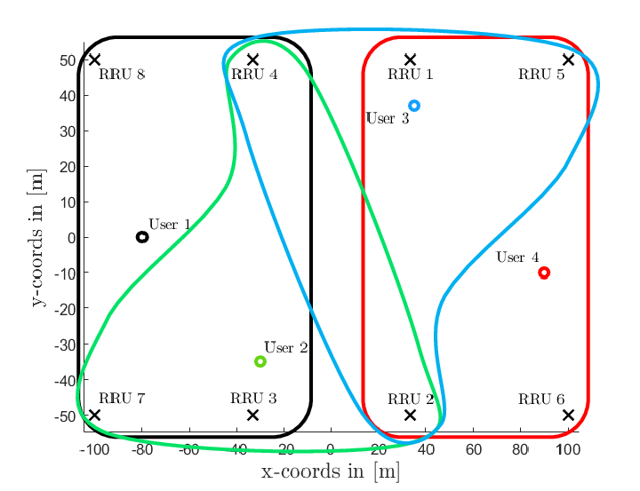
We consider a mmWave based downlink system with RRUs and each RRU is equipped with ULA of antennas. All RRUs are placed in a rectangle layout (resembling e.g., a factory-type setup) and connected to a common BBU in the edge cloud. If not mentioned otherwise, we consider JT-CoMP scenario with partially overlapping user-centric clusters, such that each active user receives a coherently synchronous signal from all RRUs in , as shown in Fig. 3 for a given channel realization. Recall that to improve communication reliability, we use parameter 99 9 The joint optimization of design parameters parameters is an interesting topic for future studies. and proactively model the SINR over the link blockage combinations (see Section III). For simplicity, let us assume , for all . All RRUs are assumed with the same maximum transmit power, i.e., for all . The AWGN noise is set to dBm/Hz, carrier-frequency GHz, and a MHz frequency band is assumed to be fully reused across all RRUs. In the simulations, we set LoS path-loss exponent , NLoS path-loss exponent , and the user priorities are set to be equal (i.e., ). All users are assumed to be randomly dropped within the coverage region, hence having different path gain and angle with respect to each RRU. By default, each antenna is equipped with a dedicated RF chain and data converters to enable fully digital signal processing. Hybrid analog-digital beamforming structures are evaluated in Section V-E. In expression (17), we use and for the subgradient and best response step sizes, respectively.
V-B Outage Performance
Fig. 4 shows the outage performance as a function of increasing blockage density for the WSRM problem.

Outage event occurs if the assigned transmit rate exceeds the achievable link rate1010 10 For a given parameter , let us denote solution obtained from the Algorithm (2). Then, for each user , the transmission rate (see Section III). However, the supported link rate of each user depends on the obtained beamformers and current channel state , which can not be exactly known to the BBU during data transmission phase due to random blockages (e.g., due to channel aging of blockage effect). Hence, the supported rates are calculated using the actual SINR values (2), i.e., , and these rates are unknown to the BBU. , for any user , i.e.,
| (18) |
It can be concluded from Fig. 4 that the outage performance is greatly improved by decreasing the subset size . Clearly, lower provides more stable and robust communication. The beamformer design with can provide reliable connectivity even if all but one LoS links are blocked. For example, with the blockage density , the outage probability is decreased from to less than by changing the parameter from to in problem (17). Thus, the specific rate allocation with can withstand blockage up to a single active LoS link, and provides greatly improved communication reliability.
When comparing the simulated results with the theoretical approximation (9), for smaller values of , the simulated outage performance appears relatively better than the theoretical counterpart, as the WSRM problem (17) solved at the BBU may end up assigning non-zero powers to only a subset of users, while all remaining users are assigned zero rate. In such a scenario, missing a LoS link results in a different blockage than what is predicted by the theoretical formula (9). Moreover, the expression (9) models the case when the channel between a RRU-user pair is either fully-available or completely blocked (e.g., both LoS and NLoS paths in (3)). However, an increase in the subset size also increases the SINR estimate (see (7)). Thus, it is likely that all users are assigned with some non-zero downlink rate, and, therefore, the simulated results tend to closely match to theoretical results obtained from (9). Furthermore, it can be seen from Fig. 4 that the proposed methods significantly outperform the conventional full-JT (), CB and MRT based beamformer designs.
V-C Effective Sum-rate Performance


Fig. 5 illustrates the trade-off between achievable sum-rate and outage performance for WSRM problem. The effective sum-rate is defined as
| (19) |
where , i.e., when each active user successfully receives the transmit data. It can be observed that when the blockage is not present (i.e., ), with the smaller subset size , the sum-rate is significantly reduced due to overly a pessimistic estimate of the aggregated SINR (see Section II-C). However, it remains relatively more stable even at much higher link blockage density due to improved communication reliability (see Fig. 4). On the other hand, with the conventional JT, the sum-rate quickly approaches zero with the slight increase in blockage density, due to higher outage. Clearly, there is a trade-off between sum-rate and outage performance, e.g., the outage performance can be improved at the small cost of achievable sum-rate. Specifically, for a given outage threshold, we can guarantee a minimum achievable sum-rate and vice versa. In addition, parameter (or in general) can be considered as an optimization or selection variable which maximizes the sum-rate for a given blockage density and outage performance, as shown in Fig. 6. The proposed methods provide robust and resilient connectivity under uncertainties of mmWave radio channel and random blockages, whereas, with the conventional full-JT (), CB and MRT methods, sum-rate rapidly decrease towards zero, even if the blockages are slightly increased.
V-D Impact of Initialization and Step Sizes


First, in Fig. 7 and Fig. 8, we examine the convergence performance of Algorithm 1 and Algorithm 2. For simplicity but without loss of generality, we consider JT-CoMP scenario with full-coordination i.e., . We set parameter and blockage density . It can be concluded that convergence is very sensitive to the choice of the step sizes . For example, with the larger value of step sizes, the algorithm can converge with a fewer number of iterations, but might result in more fluctuations to the objective. It should be noted that convergence may not necessarily be monotonic, which is an inherent feature of subgradient updates (see (17e)).
In addition, ingenious choice of the feasible initial points also impact the rate of convergence. For the considered scenario with , a simple MRT based initialization for significantly improves the convergence rate and attains near optimal solution with fewer number of iterations, as shown in Fig. 8. However, irrespective of the choice of initialization point and step sizes, both algorithms tends to converge to the local optimal solution, on the average, provided a sufficient number of iterations.
Finally, we compare the sum-rate performance of the low-complexity method based on iteratively solving a set of KKT conditions with the solution obtained directly by the optimization toolbox [49]. Moreover, with the assumption of full-CSI, (on average) the achievable performance approaches to the theoretical upper bound. It can be concluded, from Fig. 9, that Algorithm 2 achieves near-optimal performance and the resulting gap in the sum-rate performance is mainly due to insufficient convergence because of the fixed number of maximum iterations. Therefore, the proposed KKT based iterative method provides a low-complexity solution for practical implementations without any significant degradation in the achievable system performance.
V-E Hybrid Analog-Digital Beamforming Implementation
While the problem formulation and proposed solutions are generic, they can be easily extended to any multi-point configuration and dense deployments. Until now, we have restricted ourselves to the case where each antenna is equipped with a dedicated RF chain and data converter that enables fully digital signal processing. In this subsection, we provide an implementation for two-stage hybrid analog-digital architecture with coarse-level analog beamforming with a limited number of RF circuits followed by less-complex digital precoding in the digital baseband domain.
Generally, due to the high power consumption and cost of mixed-signal components in the mmWave frequencies, analog beamforming is performed using a network of phase-shifters [17, 18]. To this end, one of the common solutions in the literature is to select the analog beams from a fixed predefined codebook [17]. We assume that analog beamforming vector between a RRU-user pair () is obtained from a fixed beam steering codebook with cardinality . Furthermore, we assume that each RRU independently decides analog beamformers which maximize their local signal power, i.e., based on the following criterion:
| (20) |
Case-1: For example, let be the number of RF circuits at each RRU , then, from expression (20) we obtain . After fixing the user-specific analog beams, each RRU estimates the effective channel, i.e., for all and then computes the robust digital precoder, as explained in Section IV.
Case-2: For example, if we consider and then each RRU will have at most one active analog beam in a given direction. Therefore, aligning such a directional beam towards a specific user will degrade the achievable SNR for all other active users. However, to efficiently utilize the JT-CoMP gain, one needs to provide a comparable SNR to all the users. To do that, we first obtain a compromise transmit beam by appropriate phase-shifts and amplitude scaling to each antenna element using variable gain amplifiers [54, 55], e.g., by superimposing best beam of each user , as for all . It should be noted, in general, may not satisfy the uni-modulus constraints on beamforming coefficients [18, 34]. Optimization of the compromise multicast analog beam with and uni-modulus constraints is an interesting topic for future studies. After fixing the compromise transmit beam, each RRU estimates the effective channel, i.e., and then obtain the digital precoder, as explained in Section IV.

Fig. 10 illustrate the sum-rate performance with JT-CoMP scenario, e.g., . For simplicity but without loss of generality, we set parameter and blockage density . It can be seen that achievable sum-rate with the two-stage hybrid beamforming architecture is in general lower than full-digital beamforming. This is mainly due to dimensionality reduction of the digital precoder brought by fixed analog beamformers in the two-stage hybrid architecture. When , each RRU implements user-specific analog beam selection and achieves comparable performance to the full-digital beamforming. However, when , each RRU implements a compromise transmit beam which is aligned to all users, thus significantly reducing the achievable analog beamforming gain because of relatively wide analog beams. In addition, the overall system is DoF (DoF) limited in the digital domain, i.e., , which leads to a significant decrease in the sum-rate performance, specially in the high-SNR conditions.
In the hybrid architecture, analog beamformers are obtained from a predefined beamforming codebook (20). Thus, the computational complexity of the proposed methods mostly stems from the computation of digital precoder. It can be seen from expression (17) that computations are dominated by matrix multiplications and inversion operations in (17a). Hence, the computational complexity mainly depends on the dimension of the matrix and it is of for inverse operation [48]. Therefore, hybrid analog-digital beamforming architecture provides dimensionality reductions for digital precoder from to . Thus, the computational complexity of the matrix inverse operation is significantly reduced. As an example, the hybrid architecture provides a complexity reduction for the matrix inversion by for and , respectively. Thus, hybrid architecture achieves the better balance between complexity and system performance.
VI Conclusion
In this paper, we studied the trade-off between achievable rate and reliability in mmWave access by exploiting the multi-antenna spatial diversity and CoMP connectivity. To combat unpredictable random blockages, a pessimistic estimate of the user-specific rate is obtained over the link blockage combinations, thus providing greatly improved communication reliability. We devised a low complexity robust beamforming scheme, which is tractable for the practical implementations, based on the best response and subgradient methods, wherein, each RRU specific beamformers are optimized in parallel. Our proposed methods provide a significant reduction in the computational complexity with respect to joint optimization overall RRUs beamforming vectors. Thus, the proposed methods are scalable to any arbitrary multi-point configuration and dense deployments. Specifically, we proposed a computationally efficient iterative algorithm for the WSRM problem, based on the SCA framework and parallelization of the corresponding KKT solutions, while accounting for the uncertainties of mmWave radio channel in terms of random link blockages. Simulation results manifested the robustness of proposed beamformer design in the presence of random blockages. The outage performance and achievable throughput with the proposed methods significantly outperform the baseline scenarios and results in more stable and resilient connectivity for highly reliable mmWave communication.
Appendix A
Considering the Lagrangian in (IV-B), the stationary conditions are obtained by differentiating (IV-B) with respect to associated primal optimization variables and . After some algebraic manipulations, the stationary conditions are given as
| (21a) | ||||
| (21b) | ||||
| where is a block diagonal matrix, with all entries are zeros except for th RRU. From (21b), it can be noticed that the computational complexity scales exponentially with the length of joint beamformers (), mainly due to matrix inversion. Furthermore, all coupled and interdependent dual variables must be found simultaneously, which hinders the use of closed-form expressions. Thus, the complexity of algorithm may become intractable in practice, in particular, for dense deployments with large and . Here, instead, we implement a parallel optimization framework using the best response approach, which efficiently parallelize the beamformer updates across the distributed RRU with significantly reduced complexity as | ||||
| (21c) | ||||
where . In addition to (21) and the primal-dual feasibility constraints, the KKT conditions also include the complementary slackness conditions as given by
| (22) | ||||
| (23) |
Lets assume the user-specific priority weights (and ), then from expression (21a), we can observe
| (24) |
Thus, we can infer that at least one of dual-variables for each user is strictly positive and LHS of (24) is zero if and only if . For simplicity, (24) can be rewritten as
| (25) |
The dual-variables are coupled and interdependent due to the common SINR constraint, as also seen from (21) and (22). Therefore, it is difficult calculate the exact values of these variables in closed-form expressions. However, all the coupled non-negative Lagrangian multipliers can be iteratively solved using the subgradient method, such as based on constrained ellipsoid method. For iteration , the update for the dual variable with a small positive step size can be formulated as
| (26) |
The dual variables are initialized with small positive values. From (21c), we obtain the transmit beamformer as in expression (17a). Finally, the dual variables are chosen to satisfy the total power constraints (17c), using the bisection search method.
Appendix B
The success probability of th user in expression (8) can be upper bounded by using the binomial theorem, and defined as
| (27) |
where . In expression (27), is mean blocking probability of each user and expressed as , where
and denotes the coordinates in 2D plane. Thus, success probability can be obtained by integrating with respect to users location.
References
- [1] T. S. Rappaport, S. Sun, R. Mayzus, H. Zhao, Y. Azar, K. Wang, G. N. Wong, J. K. Schulz, M. Samimi, and F. Gutierrez, “Millimeter wave mobile communications for 5G cellular: It will work!” IEEE Access, vol. 1, pp. 335–349, 2013.
- [2] J. G. Andrews, S. Buzzi, W. Choi, S. V. Hanly, A. Lozano, A. C. K. Soong, and J. C. Zhang, “What will 5G be?” IEEE J. Sel. Areas Commun., vol. 32, no. 6, pp. 1065–1082, Jun. 2014.
- [3] G. R. MacCartney, T. S. Rappaport, and S. Rangan, “Rapid fading due to human blockage in pedestrian crowds at 5G millimeter-wave frequencies,” in Proc. IEEE Global Commun. Conf., Dec. 2017, pp. 1–7.
- [4] C. Slezak, V. Semkin, S. Andreev, Y. Koucheryavy, and S. Rangan, “Empirical effects of dynamic human-body blockage in 60 GHz communications,” IEEE Commun. Mag., vol. 56, no. 12, pp. 60–66, 2018.
- [5] A. Tölli, H. Pennanen, and P. Komulainen, “On the value of coherent and coordinated multi-cell transmission,” in Proc. IEEE Int. Conf. Commun. Workshop, Jun. 2009, pp. 1–5.
- [6] A. Tölli, M. Codreanu, and M. Juntti, “Cooperative MIMO–OFDM cellular system with soft handover between distributed base station antennas,” IEEE Trans. Wireless Commun., vol. 7, no. 4, pp. 1428–1440, Apr. 2008.
- [7] J. Wang, D. Wang, and Y. Liu, “Weighted sum rate-based coordinated beamforming in multi-cell multicast networks,” IEEE Commun. Lett., vol. 20, no. 8, pp. 1567–1570, 2016.
- [8] R. Irmer, H. Droste, P. Marsch, M. Grieger, G. Fettweis, S. Brueck, H. Mayer, L. Thiele, and V. Jungnickel, “Coordinated multipoint: Concepts, performance, and field trial results,” IEEE Commun. Mag., vol. 49, no. 2, pp. 102–111, Feb. 2011.
- [9] G. Nigam, P. Minero, and M. Haenggi, “Coordinated multipoint joint transmission in heterogeneous networks,” IEEE Trans. Commun., vol. 62, no. 11, pp. 4134–4146, Nov. 2014.
- [10] G. R. MacCartney, T. S. Rappaport, and A. Ghosh, “Base station diversity propagation measurements at 73 GHz millimeter-wave for 5G coordinated multipoint (CoMP) analysis,” in Proc. IEEE Global Commun. Conf. Workshops, Dec. 2017, pp. 1–7.
- [11] G. R. MacCartney and T. S. Rappaport, “Millimeter-wave base station diversity for 5G coordinated multipoint (CoMP) applications,” IEEE Trans. Wireless Commun., vol. 18, no. 7, pp. 3395–3410, Jul. 2019.
- [12] D. Maamari, N. Devroye, and D. Tuninetti, “Coverage in mmWave cellular networks with base station co-operation,” IEEE Trans. Wireless Commun., vol. 15, no. 4, pp. 2981–2994, Apr. 2016.
- [13] M. Gerasimenko, D. Moltchanov, M. Gapeyenko, S. Andreev, and Y. Koucheryavy, “Capacity of multiconnectivity mmWave systems with dynamic blockage and directional antennas,” IEEE Trans. Veh. Technol., vol. 68, no. 4, pp. 3534–3549, 2019.
- [14] C. Skouroumounis, C. Psomas, and I. Krikidis, “Low-complexity base station selection scheme in mmWave cellular networks,” IEEE Trans. Commun., vol. 65, no. 9, pp. 4049–4064, Sep. 2017.
- [15] C. Lee and W. Chung, “Hybrid RF-baseband precoding for cooperative multiuser massive MIMO systems with limited RF chains,” IEEE Trans. Commun., vol. 65, no. 4, pp. 1575–1589, Apr. 2017.
- [16] 3GPP TSG RAN Meeting #82, TS 37.340, “NR; Multi-connectivity; Overall description (Release 15),” Rel. 15, Jun 2018.
- [17] A. Alkhateeb, G. Leus, and R. W. Heath, “Limited feedback hybrid precoding for multi–user millimeter wave systems,” IEEE Trans. Wireless Commun., vol. 14, no. 11, pp. 6481–6494, Nov. 2015.
- [18] X. Yu, J. Shen, J. Zhang, and K. B. Letaief, “Alternating minimization algorithms for hybrid precoding in millimeter wave MIMO systems,” IEEE J. Sel. Topics Signal Process., vol. 10, no. 3, pp. 485–500, Apr. 2016.
- [19] N. A. Johansson, Y. . E. Wang, E. Eriksson, and M. Hessler, “Radio access for ultra-reliable and low-latency 5G communications,” in Proc. IEEE Int. Conf. Commun. Workshop, Jun. 2015, pp. 1184–1189.
- [20] H. Shariatmadari, Z. Li, M. A. Uusitalo, S. Iraji, and R. Jäntti, “Link adaptation design for ultra-reliable communications,” in Proc. IEEE Int. Conf. Commun., May 2016, pp. 1–5.
- [21] J. Kaleva, A. Tölli, and M. Juntti, “Decentralized sum rate maximization with QoS constraints for interfering broadcast channel via successive convex approximation,” IEEE Trans. Signal Process., vol. 64, no. 11, pp. 2788–2802, Jun. 2016.
- [22] G. Venkatraman, A. Tölli, M. Juntti, and L. Tran, “Traffic aware resource allocation schemes for multi-cell MIMO-OFDM systems,” IEEE Trans. Signal Process., vol. 64, no. 11, pp. 2730–2745, Jun. 2016.
- [23] O. Tervo, A. Tölli, M. Juntti, and L. Tran, “Energy-efficient beam coordination strategies with rate–dependent processing power,” IEEE Trans. Signal Process., vol. 65, no. 22, pp. 6097–6112, Nov. 2017.
- [24] J. Kaleva, A. Tölli, M. Juntti, R. A. Berry, and M. L. Honig, “Decentralized joint precoding with pilot-aided beamformer estimation,” IEEE Trans. Signal Process., vol. 66, no. 9, pp. 2330–2341, May 2018.
- [25] O. Tervo, L. Tran, H. Pennanen, S. Chatzinotas, B. Ottersten, and M. Juntti, “Energy-efficient multicell multigroup multicasting with joint beamforming and antenna selection,” IEEE Trans. Signal Process., vol. 66, no. 18, pp. 4904–4919, Sep. 2018.
- [26] S. Boyd, L. Xiao, and A. Mutapcic, “Subgradient methods,” lecture notes of EE392o, Stanford University, 2003.
- [27] D. Kumar, J. Kaleva, and A. Tölli, “Multi-point connectivity for reliable mmWave,” in Proc. European Sign. Process. Conf., Sep. 2019, pp. 1–5.
- [28] ——, “Rate and reliability trade-off for mmWave communication via multi-point connectivity,” in Proc. IEEE Global Commun. Conf., Dec. 2019, pp. 1–6.
- [29] A. Checko, H. L. Christiansen, Y. Yan, L. Scolari, G. Kardaras, M. S. Berger, and L. Dittmann, “Cloud RAN for mobile networks–a technology overview,” IEEE Communications Surveys Tutorials, vol. 17, no. 1, pp. 405–426, Firstquarter 2015.
- [30] T. S. Rappaport, G. R. MacCartney, M. K. Samimi, and S. Sun, “Wideband millimeter-wave propagation measurements and channel models for future wireless communication system design,” IEEE Trans. Commun., vol. 63, no. 9, pp. 3029–3056, Sep. 2015.
- [31] A. M. Sayeed, “Deconstructing multiantenna fading channels,” IEEE Trans. Signal Process., vol. 50, no. 10, pp. 2563–2579, 2002.
- [32] S. Buzzi and C. D’Andrea, “A clustered statistical MIMO millimeter wave channel model,” 2016, [Online]. Available: http://arxiv.org/abs/1604.00648.
- [33] O. E. Ayach, S. Rajagopal, S. Abu-Surra, Z. Pi, and R. W. Heath, “Spatially sparse precoding in millimeter wave MIMO systems,” IEEE Trans. Wireless Commun., vol. 13, no. 3, pp. 1499–1513, 2014.
- [34] D. Kumar, J. Saloranta, J. Kaleva, G. Destino, and A. Tölli, “Reliable positioning and mmWave communication via multi-point connectivity,” Sensors, vol. 18, no. 11, p. 4001, 2018.
- [35] M. Zhang, M. Mezzavilla, R. Ford, S. Rangan, S. Panwar, E. Mellios, D. Kong, A. Nix, and M. Zorzi, “Transport layer performance in 5G mmWave cellular,” in Proc. IEEE Int. Conf. on Comp. Commun. Workshop, Apr. 2016, pp. 730–735.
- [36] T. Bai, R. Vaze, and R. W. Heath, “Analysis of blockage effects on urban cellular networks,” IEEE Trans. Wireless Commun., vol. 13, no. 9, pp. 5070–5083, 2014.
- [37] M. Di Renzo, “Stochastic geometry modeling and analysis of multi-tier millimeter wave cellular networks,” IEEE Trans. Wireless Commun., vol. 14, no. 9, pp. 5038–5057, Sep. 2015.
- [38] E. Hriba and M. C. Valenti, “The potential gains of macrodiversity in mmWave cellular networks with correlated blocking,” in Proc. IEEE Military Commun. Conf., 2019, pp. 171–176.
- [39] E. Karipidis, N. D. Sidiropoulos, and Z. Luo, “Quality of service and max-min fair transmit beamforming to multiple cochannel multicast groups,” IEEE Trans. Signal Process., vol. 56, no. 3, pp. 1268–1279, 2008.
- [40] K. Shen and W. Yu, “Fractional programming for communication systems-—part i: Power control and beamforming,” IEEE Trans. Signal Process., vol. 66, no. 10, pp. 2616–2630, 2018.
- [41] A. A. Khan, R. S. Adve, and W. Yu, “Optimizing downlink resource allocation in multiuser MIMO networks via fractional programming and the hungarian algorithm,” IEEE Trans. Wireless Commun., vol. 19, no. 8, pp. 5162–5175, 2020.
- [42] B. R. Marks and G. P. Wright, “A general inner approximation algorithm for nonconvex mathematical programs,” Operations Research, vol. 26, no. 4, pp. 681–683, 1978.
- [43] A. Beck, A. Ben-Tal, and L. Tetruashvili, “A sequential parametric convex approximation method with applications to nonconvex truss topology design problems,” Journal of Global Optimization, vol. 47, no. 1, pp. 29–51, 2010.
- [44] J. Wang, L. Zhou, K. Yang, X. Wang, and Y. Liu, “Multicast precoding for multigateway multibeam satellite systems with feeder link interference,” IEEE Trans. Wireless Commun., vol. 18, no. 3, pp. 1637–1650, Mar. 2019.
- [45] J. Papandriopoulos and J. S. Evans, “SCALE: A low-complexity distributed protocol for spectrum balancing in multiuser DSL networks,” IEEE Trans. Inf. Theory, vol. 55, no. 8, pp. 3711–3724, Aug. 2009.
- [46] D. T. Ngo, S. Khakurel, and T. Le-Ngoc, “Joint subchannel assignment and power allocation for OFDMA femtocell networks,” IEEE Trans. Commun., vol. 13, no. 1, pp. 342–355, Jan. 2014.
- [47] T. Wang and L. Vandendorpe, “On the SCALE algorithm for multiuser multicarrier power spectrum management,” IEEE Trans. Signal Process., vol. 60, no. 9, pp. 4992–4998, Sep. 2012.
- [48] S. Boyd and L. Vandenberghe, Convex optimization. Cambridge university press, 2004.
- [49] M. Grant and S. Boyd, “CVX: Matlab software for disciplined convex programming,” http://cvxr.com/cvx, Mar. 2014.
- [50] G. Scutari, F. Facchinei, P. Song, D. P. Palomar, and J. Pang, “Decomposition by partial linearization: Parallel optimization of multi–agent systems,” IEEE Trans. Signal Process., vol. 62, no. 3, pp. 641–656, Feb. 2014.
- [51] D. Bertsekas and A. Nedic, Convex analysis and optimization. Athena Scientific, 2003.
- [52] J. Kaleva, R. Berry, M. Honig, A. Tölli, and M. Juntti, “Decentralized sum MSE minimization for coordinated multi-point transmission,” in Proc. IEEE Int. Conf. Acoust., Speech, Signal Processing, May 2014, pp. 469–473.
- [53] M. S. Lobo, L. Vandenberghe, S. Boyd, and H. Lebret, “Applications of second–order cone programming,” Linear Algebra and Applications, vol. 284, pp. 193–228, Nov. 1998.
- [54] W. Roh, J. Seol, J. Park, B. Lee, J. Lee, Y. Kim, J. Cho, K. Cheun, and F. Aryanfar, “Millimeter-wave beamforming as an enabling technology for 5G cellular communications: theoretical feasibility and prototype results,” IEEE Commun. Mag., vol. 52, no. 2, pp. 106–113, 2014.
- [55] E. Onggosanusi, M. S. Rahman, L. Guo, Y. Kwak, H. Noh, Y. Kim, S. Faxer, M. Harrison, M. Frenne, S. Grant, R. Chen, R. Tamrakar, and a. Q. Gao, “Modular and high-resolution channel state information and beam management for 5G new radio,” IEEE Commun. Mag., vol. 56, no. 3, pp. 48–55, 2018.
![[Uncaptioned image]](1910.06140v3/dileep-kumar-biopic.png) |
Dileep Kumar received the master’s degree in communication engineering from the Indian Institute of Technology Bombay (IIT Bombay), India, in 2015. He is currently pursuing the Ph.D. degree at the University of Oulu, Finland. From 2015 to 2017, he worked for NEC Corporation, Tokyo, Japan, as a Research Engineer. In 2018, he joined the Centre for Wireless Communications (CWC), University of Oulu. His research interest includes signal processing for wireless communication systems. |
![[Uncaptioned image]](1910.06140v3/jarkko-kaleva-biopic.png) |
Jarkko Kaleva (S’11-M’18) received his Dr.Sc. (Tech.) degree in communications engineering from University of Oulu, Oulu, Finland in 2018 with distinction. In 2010, he joined Centre for Wireless Communications (CWC) at University of Oulu, Finland. He is a co-founder of Solmu Technologies, where he is working as the chief software architect. His main research interests are in nonlinear programming, dynamic systems and deep learning. |
![[Uncaptioned image]](1910.06140v3/antti-tolli-biopic.png) |
Antti Tölli (M’08, SM’14) is an Associate Professor with the Centre for Wireless Communications (CWC), University of Oulu. He received the Dr.Sc. (Tech.) degree in electrical engineering from the University of Oulu, Oulu, Finland, in 2008. From 1998 to 2003, he worked at Nokia Networks as a Research Engineer and Project Manager both in Finland and Spain. In May 2014, he was granted a five year (2014-2019) Academy Research Fellow post by the Academy of Finland. During the academic year 2015-2016, he visited at EURECOM, Sophia Antipolis, France, while from August 2018 till June 2019 he was visiting at the University of California Santa Barbara, USA. He has authored numerous papers in peer-reviewed international journals and conferences and several patents all in the area of signal processing and wireless communications. His research interests include radio resource management and transceiver design for broadband wireless communications with a special emphasis on distributed interference management in heterogeneous wireless networks. He is currently serving as an Associate Editor for IEEE Transactions on Signal Processing. |