Deep Crowd-Flow Prediction in Built Environments

We formalize the problem of crowd flow prediction as follows. As raw input, we are given a matrix of unique initial agent locations $\mathbf{A}$, where agent locations are 1, and all others are zero; a corresponding matrix of shared agent goal locations $\hat{\mathbf{G}}$; and a 2D discretization of a built environment $\mathbf{E}$ into a matrix. The environment and the two location matrices have fixed dimension of $n\times n$. We use index pair $(i,j)$ to denote a location in the matrices, where $i=1..n$ and $j=1..n$. The crowd flow prediction output $\mathbf{Y}$ is the average crowd density over an entire simulation (i.e., crowd flow) for each navigable cell in environment $\mathbf{E}$.

For the agent goals, we make an assumption that each agent chooses its shared goal as the closest one. We then transform the goal locations into distance information using distance function $\mathcal{D}$, where $\mathbf{G}=\mathcal{D}(\hat{\mathbf{G}})$ converts every cell to the shortest path length from the cell to the closest goal. The resulting $\mathbf{G}$ encodes not only where goals are located (i.e., $\mathbf{G}_{i,j}=0$), but also how close an agent is to its goal. By performing a greedy search to minimize the value on $\mathbf{G}$, an agent is able to reach its goal. However, the implication of function $\mathcal{D}$ is that agents can perform pathfinding to find the shortest path to its goal, which is nearly universal in crowd simulators.

Thus far, the input encoding focused on capturing agent information. The scale of the environment is dependent on the diameter of agents, which is equal to the width of a grid cell. This means that a grid cell can represent an exact capacity of one agent per grid cell. However, there is a certain inflexibility to this representation. Namely, the dimensions $n\times n$ must be able to capture the extent of both existing and future environments, making it difficult to choose an effective $n$. We resolve this problem by altering the fixed-size agent-centric representation into a environment-centric one. We propose CAGE , an encoding and decoding technique with the capabilities to serve any environment and crowd context with unlimited size.

Given a real environment in its discretized form $\mathbf{E}$ (whose grid dimensions exceed $n\times n$), we apply a compression method that preserves environmental information. This is achieved by maintaining the local navigability (referred to as consistency) between cells, while warping their capacities (i.e., the maximum number of agents that can occupy them). For this, we require two additional “channels” of information $\mathbf{C}^{\mathbf{x}}_{n\times n}$ and $\mathbf{C}^{\mathbf{y}}_{n\times n}$ for storing capacities: one for capacity along the $x$-axis and the other for capacity along the $y$-axis. Initially both $\mathbf{C}^{\mathbf{x}}$ and $\mathbf{C}^{\mathbf{y}}$ consists of ones, meaning that each cell has a capacity of 1 agent per cell. By manipulating $\mathbf{C}^{\mathbf{x}}$ and $\mathbf{C}^{\mathbf{y}}$, regions in $\mathbf{E}$ are able to be compressed, which affects channels $\mathbf{A}$ and $\mathbf{G}$ as well. Figure 1(a) demonstrates the effect of compression on $\mathbf{C}^{\mathbf{x}}$ and $\mathbf{C}^{\mathbf{y}}$. At the yellow cell $(i,j)$, the capacity becomes $\big(\mathbf{C}^{\mathbf{x}}_{i,j}\cdot\mathbf{C}^{\mathbf{y}}_{i,j}\big)$ or 2 agents/cell, and $\mathbf{E}_{i,j}$ corresponds to a $2\times 1$ space, instead of $1\times 1$. As long as consistency is maintained, cells can have their capacities increased to other integer values. As a result, this will compress parts of the environment. A counter-example violating consistency is shown in Figure 1(b). We provide a more detailed explanation of compression in Appendix 8.1.

The changes in $\mathbf{A}$ and $\mathbf{G}$ that accompany the compression of $\mathbf{E}$ are as follows. By adding $\mathbf{C}^{\mathbf{x}}$ and $\mathbf{C}^{\mathbf{y}}$, $\mathbf{A}$ represents agent density, instead of agent locations. In Figure 1(a), the compressed yellow cell’s value in $\mathbf{A}$ becomes the number of agents among the corresponding uncompressed cells divided by the capacity of the cell. For $\mathbf{G}$, each of its cells takes on the minimum $\mathbf{G}$-value of the cells that are being compressed into the yellow cell, as this is consistent with the aforementioned use of $\mathbf{G}$ for greedy search. The resulting channels constitute the CAGE representation $\mathbf{X}=\big[\mathbf{C}^{\mathbf{x}},\mathbf{C}^{\mathbf{y}},\mathbf{A},\mathbf{G},\mathbf{E}\big]$.

After compression, the original dimensions $p\times q$ remain the same as the uncompressed environment, but there is an increase in the amount of non-navigable cells. The same outer rows and columns that are non-navigable can be removed from every channel, decreasing the dimensions of the compressed representation by $(p-n)$ along the $y$-axis and $(q-n)$ along the $x$-axis. This encoding technique is now equipped to represent an infinite number of compressed environments within $n\times n$.

After the crowd density $\mathbf{Y}$ is predicted on the compressed representation $\mathbf{X}$, decompression can be achieved by having temporarily stored both the original and compressed locations and sizes of each region $\hat{R}\in R$. The compressed information locates the region’s data from $\mathbf{C}^{\mathbf{x}}$, $\mathbf{C}^{\mathbf{y}}$, and $\mathbf{Y}$, and the original information delimits where the data should be decompressed to. In order to expand a region to its original size, the density predicted in each cell $(i,j)$ will be uniformly divided across $\big(\mathbf{C}^{\mathbf{x}}_{i,j}\cdot\mathbf{C}^{\mathbf{y}}_{i,j}\big)$-many cells, which comprised cell $(i,j)$ after compression.

The components of the CAGE representation define the dataset’s input $X$ of initial conditions. For the environmental component $\mathbf{E}$, we utilize a multi-phase generation of floorplans for built environments with no small obstacles. This is based on a floorplan typology observed in modern architecture by Dogan et al [6], which we repurpose for floorplan generation instead of classification. The three stages of generation are (a) forming an exterior shape to the floorplan, (b) applying an interior organization of hallways, and (c) populating the floorplan with rooms interconnected toward the closest hallways.

The generated floorplans must then be accompanied by both the other input components in the CAGE representation and the ground truth crowd flow $\hat{\mathbf{Y}}$. In the dataset, the number of agents and the type of crowd flow output create four major groups, each of which have a uniform distribution of floorplan types (Figure 2). Namely, each group is a combination of either sparse or dense crowds and either proxy or simulated crowd flow. The separation of sparse crowds from dense crowds is motivated by the visual differences between their respective crowd flows. When there are relatively few agents (e.g., $\leq$ 25 agents), the crowd flow is constituted of the fine paths that agents travelled along, which likens the prediction of crowd flow to finding the shortest paths from the agents to their goals (i.e., the long-term micro-predictions described in Section 2). On the contrary, when there are relatively many agents (e.g., $\geq$ 0.01 agents/m²), the crowd flow becomes stigmergic, where the focus on the individual is lost when its joins the crowd (i.e., long-term macro-predictions).

In this work, the proxy crowd flow is realized through static generation, as opposed to dynamic generation by means of a crowd simulator for simulated crowd flow (in this case, the social force model [8]). This crowd flow serves as a proxy for simulated crowd flow and makes the generation of data is made significantly faster. Compared to that of the simulated crowd flow, its visual features are less fine, which simplifies the prediction problem. For sparse crowds, proxy crowd flow is generated by overlaying the shortest paths from individual agents to their goals (Figure 4). For dense crowds, cohesive groups of agents have their group paths overlaid (Figure 2). The resulting difference between sparse crowds and dense crowds is that group paths capture the congestion caused by bottlenecks, while individual paths do not.

In order to evaluate the quality of the predictions for each model on its corresponding dataset, we compare the cell-wise differences between the predicted crowd flow and the ground truth crowd flow.

The metrics included in Table 1 are $MAE$ and Kullback-–Leibler divergence ($D_{KL}$). For the $\mathbf{E}$-centric goals, low $MAE$ is indicative of good performance. This score highlights the success of Mono-SegNet , and thereby Dual-SegNet , since Dual-SegNet utilizes Mono-SegNet for its predictions of dense crowds. For the $\mathbf{G}$-centric goals, $MAE$ cannot be considered in the same way, because the ground truth crowd flow is comparatively sparse to that of $\mathbf{E}$-centric goals. If, for instance, a predictor outputs no density, the $MAE$ for the $\mathbf{G}$-centric goal will be inherently lower than for the $\mathbf{E}$-centric goal. Therefore, $D_{KL}$ is needed to gain better insight into the $\mathbf{G}$-centric goals. A low $D_{KL}$ indicates that the predicted crowd flow is concentrated over where the ground truth crowd flow would be.This shows that despite having a low $MAE$, Mono-SegNet performs poorly for the $\mathbf{G}$-centric goal, because the $D_{KL}$ is high. On the other hand, the $D_{KL}$ of Dual-SegNet is comparatively lower, evidencing its good performance for the $\mathbf{G}$-centric goal.

The quantitative evaluation provides insights at large, but the capabilities of our models are also well-conveyed through visual comparisons between predictions and ground truth. Figure 4 shows the results of the two models for the $\mathbf{E}$- and $\mathbf{G}$-centric goals. Although there are four goals defined in Table 1, Dual-SegNet utilizes Mono-SegNet for its $\mathbf{E}$-centric goal, so it was not given a row in Figure 4.

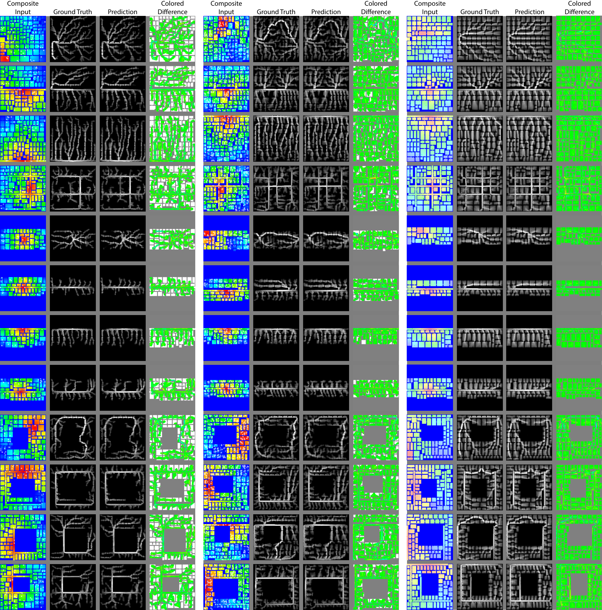
The performance observed in Table 1 is well-evidenced by the results in Figure 4, which shows from left to right: the input, ground truth, prediction, and difference between the ground truth and prediction. Although the input is encoded in the CAGE representation, its $\mathbf{A}$, $\mathbf{G}$, and $\mathbf{E}$ components are able to be composited. $\mathbf{G}$ appears to visually encode $\mathbf{E}$, so it was used in place of $\mathbf{E}$ and combined with the agent locations in $\mathbf{A}$ (in white). In order to improve contrast between $\mathbf{G}$ and $\mathbf{A}$, $\mathbf{G}$ was converted into a heatmap, where the red hue is closest to the goal. The difference between the ground truth and prediction is visualized by a Colored Difference image. When the predicted crowd flow is equivalent to the ground truth crowd flow and non-zero, the hue is green. As the prediction diverges, its hue becomes either more blue (when it underpredicts the crowd flow) or more yellow (when it produces a phantom crowd flow).

From top to bottom in Figure 4, starting with Mono-SegNet and Dual-SegNet ’s $\mathbf{E}$-centric goal, the positive performance is conveyed by the abundance of green. This is can also be confirmed by viewing the ground truth and prediction images separately. Meanwhile, Mono-SegNet ’s $\mathbf{G}$-centric goal was unsuccessful, as depicted by the Colored Difference, wherein the entire ground truth flow is colored a vivid blue. After having trained a separate model only for its $\mathbf{G}$-centric goal, Dual-SegNet shows excellent performance in predicting not only the path of one agent, but also those of numerous others. These fine paths are highlighted in green, and there is very little phantom crowd flow. Appendix 8.2 and 8.3 showcase numerous compelling test results for dense and sparse crowds respectively.

Given a real environment in its discretized form $\mathbf{E}$ (whose dimensions exceed $n\times n$), let us apply a visibility function $\mathcal{V}$ which for each navigable cell $(i,j)$ in $\mathbf{E}$, assigns a tuple

where $\mathbf{x}=[1,0]$, $\mathbf{y}=[0,1]$ are unit vectors, and function $\mathcal{N}(i,j)_{\mathbf{b}}$ computes the number of navigable cells visible from $(i,j)$ along the unit vector $\mathbf{b}$ (see two examples in Figure 5). Then, $\mathcal{V}(\mathbf{E})$ has segmented $\mathbf{E}$ into a set of regions $R$ where the tuple values of each region’s cells are the same. The purpose of using the visibility function is to encode navigability in the environment along the coordinate axes. Thereby, each region $\hat{R}\in R$ represents a maximal unit of space (or maximal set of neighboring cells) that is similarly navigable and therefore compressible (Figure 5). A region’s width and height are represented by $\hat{R}^{\mathbf{x}}$ and $\hat{R}^{\mathbf{y}}$ respectively, and denoted as the number of cells along each of the axis.

Two constraints are needed to ensure that compression is consistent. Namely, for any two regions $\hat{R}_{i}$ and $\hat{R}_{j}$, if they are contiguous along axis $\mathbf{b}$, they must (Constraint 1) have the same value for $\mathbf{C}^{\bot\mathbf{b}}$ along the orthogonal axis $\bot\mathbf{b}$ and (Constraint 2) have the same region length along axis $\bot\mathbf{b}$ (i.e., $\hat{R}_{i}^{\bot\mathbf{b}}=\hat{R}_{j}^{\bot\mathbf{b}}$). These constraints ensure that neither visibility nor navigability are disrupted by compression.

References

- [1] A. Alahi, K. Goel, V. Ramanathan, A. Robicquet, L. Fei-Fei, and S. Savarese. Social lstm: Human trajectory prediction in crowded spaces. In Proceedings of the IEEE conference on computer vision and pattern recognition, pages 961–971, 2016.
- [2] J. Amirian, J.-B. Hayet, and J. Pettre. Social ways: Learning multi-modal distributions of pedestrian trajectories with gans. In The IEEE Conference on Computer Vision and Pattern Recognition (CVPR) Workshops, June 2019.
- [3] V. Badrinarayanan, A. Kendall, and R. Cipolla. Segnet: A deep convolutional encoder-decoder architecture for image segmentation. CoRR, abs/1511.00561, 2015.
- [4] L. Boominathan, S. S. Kruthiventi, and R. V. Babu. Crowdnet: A deep convolutional network for dense crowd counting. In Proceedings of the 24th ACM international conference on Multimedia, pages 640–644. ACM, 2016.
- [5] L. Bottou. Large-scale machine learning with stochastic gradient descent. In Proceedings of COMPSTAT’2010, pages 177–186. Springer, 2010.
- [6] T. Dogan, E. Saratsis, and C. Reinhart. The optimization potential of floor-plan typologies in early design energy modeling. 12 2015.
- [7] K. He, X. Zhang, S. Ren, and J. Sun. Delving deep into rectifiers: Surpassing human-level performance on imagenet classification. In Proceedings of the IEEE international conference on computer vision, pages 1026–1034, 2015.
- [8] D. Helbing and P. Molnár. Social force model for pedestrian dynamics. Phys. Rev. E, 51:4282–4286, May 1995.
- [9] G. Huang, Z. Liu, L. Van Der Maaten, and K. Q. Weinberger. Densely connected convolutional networks. In Proceedings of the IEEE conference on computer vision and pattern recognition, pages 4700–4708, 2017.
- [10] S. Huang, X. Li, Z. Zhang, F. Wu, S. Gao, R. Ji, and J. Han. Body structure aware deep crowd counting. IEEE Transactions on Image Processing, 27(3):1049–1059, 2017.
- [11] R. Jiang, X. Song, D. Huang, X. Song, T. Xia, Z. Cai, Z. Wang, K.-S. Kim, and R. Shibasaki. Deepurbanevent: A system for predicting citywide crowd dynamics at big events. In Proceedings of the 25th ACM SIGKDD International Conference on Knowledge Discovery & Data Mining, pages 2114–2122. ACM, 2019.
- [12] W. Jin, Y. Lin, Z. Wu, and H. Wan. Spatio-temporal recurrent convolutional networks for citywide short-term crowd flows prediction. In Proceedings of the 2nd International Conference on Compute and Data Analysis, pages 28–35. ACM, 2018.
- [13] Y. LeCun, B. Boser, J. S. Denker, D. Henderson, R. E. Howard, W. Hubbard, and L. D. Jackel. Backpropagation applied to handwritten zip code recognition. Neural computation, 1(4):541–551, 1989.
- [14] J. Liu, C. Gao, D. Meng, and A. G. Hauptmann. Decidenet: Counting varying density crowds through attention guided detection and density estimation. In Proceedings of the IEEE Conference on Computer Vision and Pattern Recognition, pages 5197–5206, 2018.
- [15] W. Luo, B. Yang, and R. Urtasun. Fast and furious: Real time end-to-end 3d detection, tracking and motion forecasting with a single convolutional net. In Proceedings of the IEEE conference on Computer Vision and Pattern Recognition, pages 3569–3577, 2018.
- [16] A. Rudenko, L. Palmieri, M. Herman, K. M. Kitani, D. M. Gavrila, and K. O. Arras. Human motion trajectory prediction: A survey. arXiv preprint arXiv:1905.06113, 2019.
- [17] V. Sindagi and V. M. Patel. A survey of recent advances in cnn-based single image crowd counting and density estimation. CoRR, abs/1707.01202, 2017.
- [18] G. Tripathi, K. Singh, and D. K. Vishwakarma. Convolutional neural networks for crowd behaviour analysis: a survey. The Visual Computer, 35(5):753–776, 2019.
- [19] D. Wolinski, M. C. Lin, and J. Pettré. Warpdriver: Context-aware probabilistic motion prediction for crowd simulation. ACM Trans. Graph., 35(6):164:1–164:11, Nov. 2016.
- [20] S. Yi, H. Li, and X. Wang. Pedestrian behavior understanding and prediction with deep neural networks. In European Conference on Computer Vision, pages 263–279. Springer, 2016.
- [21] B. Yogameena and C. Nagananthini. Computer vision based crowd disaster avoidance system: A survey. International journal of disaster risk reduction, 22:95–129, 2017.
- [22] J. Zhang, K. J. Shih, A. Elgammal, A. Tao, and B. Catanzaro. Graphical contrastive losses for scene graph parsing. In Proceedings of the IEEE Conference on Computer Vision and Pattern Recognition, pages 11535–11543, 2019.
- [23] J. Zhang, Y. Zheng, and D. Qi. Deep spatio-temporal residual networks for citywide crowd flows prediction. In Thirty-First AAAI Conference on Artificial Intelligence, 2017.
- [24] A. Zonoozi, J. jae Kim, X. li Li, and G. Cong. Periodic-crn: A convolutional recurrent model for crowd density prediction with recurring periodic patterns. In IJCAI, 2018.
8 Appendix
8.1 CAGE Compression Method