Development of data-analysis software
for total-reflection high-energy positron diffraction (TRHEPD)
Abstract
The present paper reports on the recent activity of the data analysis software development for total-reflection high-energy positron diffraction (TRHEPD), a novel experimental technique for surface structure determination. Experiments using TRHEPD are being conducted intensively at the Slow Positron Facility, Institute of Materials Structure Science, High Energy Accelerator Research Organization, revealing surface structure of interest. The data analysis software provides a solution to the inverse problem in which the atomic positions of a surface structure are determined from the experimental diffraction data (rocking curve). The forward problem is solved by the numerical solution of the partial differential equation in the quantum scattering problem. A technical demonstration with a test problem was carried out to confirm the software functioned as expected. Since the analysis method has a general mathematical foundation, it is also applicable to other experiments, such as X-ray or electron diffraction experiments.
PACS 07.78.+s, 14.60.Cd, 68.35.Bs
1 Introduction
Since material properties are governed by the atomic structure or the type and position of each atom, the information of the structure is critical in discerning these properties. For bulk structure, X-ray diffraction is the standard technique used to determine the structure of the crystals of new materials, proteins, and so on. For surface structure, however, a standard technique for the definitive determination of the atomic structure of the topmost and subsurface atoms is not yet established.
Total-reflection high-energy positron diffraction (TRHEPD) has been developed as a novel method for such surface structure determination. At the Slow Positron Facility (SPF), Institute of Materials Structure Science (IMSS), High Energy Accelerator Research Organization (KEK) much work has been conducted, successfully and revealing surface structures of the surfaces of interest. (see a review [1]). For example, TRHEPD determined the structure of the rutile-TiO2(110) (1 2) surface which had been under debate over 30 years [2].
Here, we report recent activity on the software development for the analysis of TRHEPD data. It is based on the inverse problem in which the surface structure is determined from the experimental diffraction data.
The present paper is organized as follows: experiment and theory of TRHEPD is explained briefly in Section 2; overview of the data analysis software is presented in Section 3; Section 4 details the technical demonstration of the software and associated discussions; a summary and a future aspect is given in Section 5.

2 TRHEPD
Features of TRHEPD are shown schematically in Figure 1 and will be briefly explained in this section. The experimental basis is the same as in reflection high-energy electron diffraction (RHEED) experiments.
The problem is to determine the positions of the atoms at the top-most surface layer and several subsurface layers. Hereafter, the axis is assumed to be perpendicular to the material surface and the coordinates are denoted as . is the number of the atoms of which positions will be determined through the data analysis.
The data analysis provides a solution to the inverse problem in which the surface structure, , is determined from the experimental diffraction data . The calculated diffraction data is obtained from the position of the atoms [3] and the calculation is called the forward problem .
2.1 Experiment
The TRHEPD experiment is shown schematically in Figure 1(a). We also define the incident wave vector projected on the - plane, where is the positron wave number in the vacuum. The incident wave direction is characterized by the glancing angle and the azimuthal angle .
Diffraction spots on the screen in Figure 1(a) are characterized by the two-dimensional indices of reciprocal lattice rods. The intensity of the specific spots, , is observed as a function of the incident glancing angle, (), and called the rocking curve. The rocking curve, , depends also on the azimuthal angle , which is fixed during a rocking curve measurement. The spot with the indices of is usually brightest and called 00 spot. This paper focuses on the 00 spot and we will drop the indices for simplicity (). The observed data among discrete glancing angles is denoted as , where a typical number of the glancing angles is 50 - 100. The present data analysis is carried out by the normalized vector data () and similarly normalized calculated values.
It is important that the rocking curve with a given azimuthal angle is hardly affected by the atomic coordinate parallel to the vector . If the vector is parallel to the -axis, for example, the rocking curve depends only on the and components of the atomic position (). In addition, one can choose the azimuthal angle intentionally shifted from any high-symmetry zone axes so that the rocking curve practically depends only on the components of the atomic position () - this is called a one-beam condition [4]. Another choice for the azimuthal angle is that it is set along a high-symmetry zone axis - this is called a many-beam condition. These properties allow us to reduce the number of variables in the data analysis from to . Such dimensional reduction is of great advantage in realizing fast and reliable data analysis.
Therefore, the measurement procedure, typically, consists of two stages, where three diffraction data sets at different azimuthal angles are obtained. One data set is provided by an experiment in a one-beam condition, which is denoted as . The other two sets are provided by experiments in the many-beam condition, which are denoted as and . Mutually orthogonal incident wave vectors were chosen for the two data sets under the many-beam condition. The first stage of the analysis procedure determines the component of the atomic position from the data set in the one-beam condition . The second stage determines the two components on the - plane, and coordinates from the other two data sets each in the many-beam condition , in which analysis the z components determined in the first stage are fixed.
2.2 Theory
The theory or the forward problem of TRHEPD [3] is based on the quantum scattering problem of the positron wavefunction ; the situation is shown schematically in Figure 1(b). The partial differential equation with a given glancing angle and an azimuthal angle
| (1) |
is solved numerically, so as to obtain rocking curve data . Here is the crystal potential determined by the atomic positions . The crystal potential is periodic on the - plane and can be written by the two-dimensional Fourier series
| (2) |
where () is the surface reciprocal lattice vector of the th rod (). In the numerical calculation [3], the coordinate is discretized by the mesh grid with an equi-interval (). A typical value of the mesh interval is Å.
The calculation under the one-beam condition [4] is much faster than that under the many-beam condition, since under the one-beam condition, the only one Fourier component is non-zero in equation (2)
| (3) |
In this case, the wavefunction can also be written as and equation (1) is reduced to a one-dimensional scattering problem
| (4) |
It is noted that this calculation method [3] was originally developed for electron diffraction (RHEED) but is applicable, since the TRHEPD method is different from that for RHEED only in the sign of the incident-particle charge. As the electron beam penetrates into deeper layers than the positron, owing to the refraction off the surface, as schematically shown in Figure 1(b), electron diffraction is less sensitive to surface structure than the positron diffraction.
3 Data analysis method
This section details the method used for the data analysis or the inverse problem . The inverse problem is solved by optimizing the residual function between the calculated and experimental diffraction data
| (5) |
with a given experimental diffraction data , where is also normalized (). The function is called the reliability factor or R-factor.
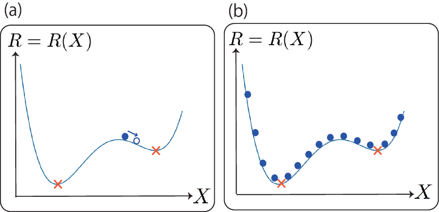
In general, optimization algorithms are classified into local or global searches. Two typical algorithms are illustrated in Figure 2; Figure 2(a) shows a local search algorithm with iterative updates, in which an initial structure data is prepared and the data, , is updated iteratively (), so as to decrease . Figure 2(b), on the other hand, shows a global search algorithm with a straightforward calculation on a mesh grid, which will be discussed later in Section 4.2.
The present paper focuses
on a local search algorithm.
The iterative optimization is realized using the
Nelder-Mead algorithm
[6, 7],
a commonly used gradient-free optimization algorithm,
where
the gradient () is not calculated in any way.
The iterative process is stopped
when it reaches a convergence criteria chosen by the user.
In this study, we developed a Python-based data analysis software.
The Nelder-Mead algorithm is realized
by the module in the scipy library (scipy.optimize.fmin).
The method is standard and the use of the scipy library is not essential.


4 Technical demonstration and discussion
4.1 Technical demonstration
A numerical test problem was run for the technical demonstration of our data analysis software. The test problem used was to reproduce the Si(001)- surface structure. Studies of this structure, shown in Figure 3, have been reported in a number of papers, such as Reference [8]. The two top-most silicon atoms form an asymmetric dimer, where the coordinate values of these atoms differ significantly. The higher (vacuum-side) atom and the lower (bulk-side) atom of the surface dimer are denoted as Si(high) and Si(low), respectively. The asymmetry is induced to decrease total surface energy by the electron transfer from Si(low) to Si(high), which results in a lone pair in the dangling-bond state at Si(high) and an empty dangling-bond state at Si(low). The coordinates of the higher and lower atoms are denoted by and in Figure 3, respectively, where the origin of the axis () is located at the plane of the atoms in the second surface layer.
In the present demonstration, the values of the component of the two top-most silicon atoms are determined from the diffraction data in the one-beam condition. A numerically generated ‘reference’ data is used, instead of a real experimental data . The reference data is generated numerically for the known structure ()) and the R-factor is defined as
| (6) |
where = (1.5832 Å, 0.8603 Å). A demonstration with the numerically generated reference data was carried out in order to confirm that the Nelder-Mead algorithm was suitable and reached the exact solution . When analyzing with experimental data, an optimized value of is usually acceptable in surface structure determination research.
The analysis results are summarized in Figures 4 and 5. Figure 4 shows the iterative optimization process. The R-factor and the coordinates of the surface atoms are plotted as functions of the iteration step , in Figure 4 (a) and (b), respectively. Figures 4 and 5 indicate that the structure converges to the exact solution correctly. The R-factor changes from at the initial structure () into at the final structure (). Figure 5 shows the rocking curve in the initial and final structure, where the reference data is also shown. Figure 5 confirms that the atomic coordinates obtained by the search reproduce the reference data correctly. The analysis was carried out on a notebook PC with an Intel CoreTM i3-6006U processor and the elapsed time was 72 s, including the computational time and the file I/O time.
It is of note that the difference in the atomic positions between the initial and the final structures is of the order of Å in Figure 4(b) and the difference can be clearly observed in the rocking curves of Figure 5. This demonstrates that TRHEPD can give an excellent selectivity or an ultra-fine spatial resolution in the order of Å, if the experimental uncertainty of the observed data is sufficiently small.
4.2 Discussion
A number of issues are discussed below on the current and prospective versions of the data analysis software. (I) The present paper has detailed a technical demonstration of the software. Data analysis with real experiment is ongoing. (II) The forward problem solver code used is planned to be parallelized for faster computation. Since the computations of the intensity with different numbers are independent, the procedure is ideal for parallelism on current computers. (III) Work is underway to develop further software with the global search algorithm shown in Figure 2, so as to avoid the local, not absolute, optimization. The software presently used provides an iterative optimization algorithm and requires an initial guess for the structure. As such, the analysis is based on a local search algorithm and can be trapped by a local minimum of . A simple-comparison algorithm may require significant computational cost because the number of sets of atomic coordinates increases exponentially with the increasing number of atoms and in reducing the mesh in the coordinates. However, this type of algorithm is suitable for modern massive parallel supercomputers as the calculations of among different atomic positions, , of different atoms are independent procedures. Our global search software is now being tested on several supercomputers, such as the Oakforest-PACS supercomputer in Japan. (IV) In addition, we plan to develop another global search method based on Besian inference with a Monte Carlo (stochastic) algorithm. The Monte Carlo algorithm is known as a reliable and efficient sampling method. The method provides the posterior probability of atomic positions through Bayes’ theorem and enables us to evaluate the uncertainty of estimated atomic positions. This method has been applied to surface structure analysis by X-ray diffraction experimentation [9].
5 Summary and future aspect
A data analysis software is being developed for surface structure analysis by the total-reflection high-energy positron diffraction (TRHEPD). The software provides a solution to the inverse problem, where the forward problem is a quantum scattering problem or partial differential equation. The software has a solid mathematical foundation and shows promise for the analysis of real experimental data. The program code will be available online in the near future.
As a future aspect, the software will be promoted to address general data analysis of surface structures, not only for positron diffraction but also for X-ray and electron diffraction by simply changing the forward problem solver.
Acknowledgement
The present research is supported by the Japanese government in the post-K project and KAKENHI funds (19H04125, 17H02828). Several numerical computations were carried out by the supercomputer Oakforest-PACS supercomputer for the Initiative on Promotion of Supercomputing for Young or Women Researchers, Information Technology Center, The University of Tokyo, the HPCI project (hp190066) and Interdisciplinary Computational Science Program in the Center for Computational Sciences, University of Tsukuba. Several computations were carried out also on the facilities of the Supercomputer Center, the Institute for Solid State Physics, the University of Tokyo and the Academic Center for Computing and Media Studies, Kyoto University.
References
- [1] Y. Fukaya, A. Kawasuso, A. Ichimiya and T. Hyodo, J. Phys. D 52, 013002/1-19 (2018).
- [2] I. Mochizuki, H. Ariga, Y. Fukaya, K. Wada, M. Maekawa, A. Kawasuso, T. Shidara, K. Asakura, and T. Hyodo, Phys. Chem. Chem. Phys. 18, 7085–7092 (2016).
- [3] A. Ichimiya, Jpn. J. Appl. Phys. 22, 176–180 (1983).
- [4] A. Ichimiya, Surf. Sci. 192, L893–L898 (1983).
- [5] T. Hanada, H. Daimon, and S. Ino. Phys. Rev. B 51, 13320–13325 (1995).
- [6] A. John Nelder and R. Mead, Computer Journal 7, 308–313 (1965).
- [7] J. C. Lagarias, J. A. Reeds, M. H. Wright, and P. E. Wright, SIAM J. Opt. 9, 112–147 (1998)
- [8] A. A. Stekolnikov, J. Furthmüller and F. Bechstedt, Phys. Rev. B 65, 115318/1-10 (2002).
- [9] M. Anada, Y. Nakanishi-Ohno, M. Okada, T. Kimura, and Y. Wakabayashi, J. Appl. Cryst. 50, 1611–1616 (2017).