Regression for Copula-linked Compound Distributions with Applications in Modeling Aggregate Insurance Claims
Abstract
In actuarial research, a task of particular interest and importance is to predict the loss cost for individual risks so that informative decisions are made in various insurance operations such as underwriting, ratemaking, and capital management. The loss cost is typically viewed to follow a compound distribution where the summation of the severity variables is stopped by the frequency variable. A challenging issue in modeling such outcome is to accommodate the potential dependence between the number of claims and the size of each individual claim. In this article, we introduce a novel regression framework for compound distributions that uses a copula to accommodate the association between the frequency and the severity variables, and thus allows for arbitrary dependence between the two components. We further show that the new model is very flexible and is easily modified to account for incomplete data due to censoring or truncation. The flexibility of the proposed model is illustrated using both simulated and real data sets. In the analysis of granular claims data from property insurance, we find substantive negative relationship between the number and the size of insurance claims. In addition, we demonstrate that ignoring the frequency-severity association could lead to biased decision-making in insurance operations.
Keywords: Aggregate insurance claims, Compound distributions, Copula regression, Incomplete data, Two-part models
1 Introduction
In actuarial research on nonlife insurance, a task of particular interest and importance is to predict the loss cost for individual risks in an insurer’s book of business. Interpretation and prediction of loss cost of individual policyholders deepens the insurer’s understanding of the risk profile of the entire portfolio, which further leads to better-informed decisions in various insurance operations such as underwriting, ratemaking, and capital management.
The loss cost of a policyholder is jointly determined by the number of claims and the amount of each claim during the contract period. As a result, researchers and practitioners typically view the loss cost outcome to follow a compound or generalized distribution (see Karlis and Xekalaki 2005 and Johnson et al. 2005). Specifically, the loss cost per policy year, denoted by , can be represented as:
| (1) |
where is a counting random variable and represents the number of claims, and () is a non-negative continuous random variable and represents the size of the th claim. The sequence of is further assumed to be independently and identically distributed. Compound distributions have been extensively used in the actuarial science literature for modeling aggregate losses in an insurance system (see, for example, Klugman et al. 2012, Lin 2014, and Albrecher et al. 2017). In insurance applications, and are referred to as the “frequency” and “severity” components respectively.
In this article, we focus on the regression method for compound distributions when both and are observed. A challenging issue in modeling such outcomes in the regression setting is to accommodate the potential dependence between the number of claims and the size of each individual claim. The goal of this work is to introduce a simple yet flexible regression framework to allow for arbitrary dependence between the frequency and severity distributions.
The current regression approach to studying the aggregate loss relies on the independence assumption between and each . Under such independence assumption, one develops regression models for the number and size of claims separately, which is known as the frequency-severity or two-part model. See Frees 2014 for discussions on various types of two-part models. As a special case, when the frequency is a Poisson variable and the severity is a gamma variable, the loss cost is known to follow a Tweedie distribution (Tweedie 1984). Jørgensen and de Souza 1994 and Smyth and Jørgensen 2002 have explored fitting the Tweedie’s compound Poisson model to the loss cost data in property insurance.
In addition to actuarial science and insurance, regression models based on compound distributions have been used in many other disciplines as well. In health economics, the two-part model was used to study an individual’s total number of doctor visits resulting from multiple spells of illness in a given period (see, for instance, Silva and Windmeijer 2001). In marketing, Tellis 1988 employed a special case of the frequency-severity model to study the effect of repetitive advertising on consumer purchasing choices; Aribarg et al. 2010 studied consumer advertisement recognition where an individual’s attention is formulated as a compound model determined by eye fixation frequency and gaze duration. In operational risk, the compound distribution for aggregate losses is the foundation for the determination of the operational risk capital required by the Basel capital framework for banks (Panjer 2006 and Shevchenko 2010). In psychology, Smithson and Shou 2014 pointed out the applications of this type of model in different areas of psychology such as perception and decision making, where a psychological process is thought to be serially summed from observable component process outputs.
The two-part models in different scientific fields described above employ some common key assumptions, including:
- (1)
The distribution of does not depend on the values of for ;
- (2)
Conditional on , are independently distributed random variables;
- (3)
Conditional on , the common distribution of does not depend on .
The (conditional) independence assumption between and certainly leads to tractable statistical inference because it allows one to build regression models separately for the frequency and severity components. However, if and are correlated, ignoring the association between them will lead to serious biases in the inference. First, the regression coefficients in the severity regression model will be inconsistent estimates of the marginal effect of explanatory variables. Second, there is a persistent error in the prediction for the severity given the frequency. Third, the misspecification will introduce bias in the inference for the compound distribution.
Motivated by the above observations, we introduce a novel copula-linked compound distribution and the associated two-part regression framework that allow for arbitrary dependence between the frequency and severity components. Specifically, we employ a parametric copula to construct the joint distribution of frequency and severity variables, thus relax the independence assumption in standard methods. We show that the resulting copula regression framework is able to nest several commonly used approaches as special cases, including the hurdle model, the selection model, and the frequency-severity model, among others. Furthermore, we extend the basic model to accommodate the case of incomplete data due to censoring or truncation. Because of the parametric nature, likelihood-based approaches are proposed for estimation, inference, and diagnostics.
The flexibility of the proposed model is illustrated using both simulated and real data sets. In the numerical experiments, we showcase the impact of ignoring the frequency and severity dependence on the resulting compound distribution. In the empirical study, we apply the proposed method to granular claims data in property insurance. Our analysis detects substantive negative dependency between the number and the size of insurance claims. In addition, we demonstrate the importance of such dependency in some key insurance functions, including underwriting and ratemaking, loss reserving, and capital management. The results suggest that ignorance of frequency-severity dependence could lead to biased decision-making in insurance operations.
To the best of our knowledge, this work is among the first efforts to explicitly incorporate the dependence between the frequency and severity variables of a compound distribution in a regression setting. Recent literature has made some development in this direction, for example, see Czado et al. 2012, Krämer et al. 2013, and Garrido et al. 2016 among others. The fundamental difference between our work and existing studies is that the aforementioned studies examined the relation between the frequency and the average severity , while the proposed method directly looks into the relation between the frequency and the individual severity . Alternative mechanisms for introducing dependence between the frequency and individual severity variables include the correlated random-effect framework as in Olsen and Schafer 2001 and the conditional approach as in Frees et al. 2011. The difficulty with both methods compared to the proposed copula approach is that it is not straightforward to handle incomplete data which is not unusual in insurance applications because of various coverage modifications.
Given that our work fits in the broader literature on multivariate modeling in insurance, it is worth discussing their differences and connections. The current literature on dependence modeling of insurance claims focuses on the joint modeling of multiple outcomes of loss cost that could arise from multiple lines of business (see Frees et al. 2016), multiple coverage in a single business line (see Shi et al. 2016), or multiple peril types covered by a policy (see Shi and Yang 2018). In this line of studies, each loss cost outcome is formulated using either a Tweedie model or a two-part model. Both can be viewed in the framework of the compound distribution (1) where the and each are assumed to be independent with each other. Apart from the association among multiple loss cost outcomes, this work examines a single loss cost outcome, and the focus is on the dependence between the frequency and severity components in the compound model.
The rest of the paper is structured as follows. Section 2 introduces the dependent frequency-severity regression model for the compound distribution and discusses its extension for incomplete data due to censoring and truncation. The likelihood-based methods for estimation, inference, and diagnostics are further discussed. Section 3 provides numerical experiments to show the impact of ignoring the frequency-severity dependence under various settings. Section 4 applies the proposed approach to the loss cost data in property insurance and shows the importance of the frequency-severity dependence in insurance operations. Section 5 concludes the article. The supplementary materials contain additional technical examples, numerical studies, and detailed data analysis.
2 Copula-linked Compound Regression
2.1 Basic Model
In the basic setup, we assume that complete information on is observed for each subject, where is a count variable, and are continuous variables. For simplicity, we suppress the subject index in the following presentation. The joint distribution of is built upon the assumption that are conditionally i.i.d. given as opposed to the unconditional i.i.d. assumption in the standard compound distribution. There are several implications of this assumption. First, conditional independence of given introduces correlation among , which departs from the i.i.d. assumption in the standard model; Second, identical distribution of given implies identical marginal distribution of , which is consistent with the i.i.d. assumption in the standard model; Third, the bivariate distribution of are identical given , which nests the independent case in the standard model.
To facilitate presentation, we denote as the variable associated with the common distribution of the sequence . Note that is only defined in the sense of a distribution, not in the sense of a random variable. Under the conditional independence assumption, the associated pmf/pdf function is:
| (4) |
where is an indictor function.
The central component to define (4) is the joint distribution of and . To allow for flexible dependence between and , we take a parametric approach and employ a bivariate parametric copula to construct their joint distribution. Refer to Nelsen 2006 and Joe 2014 for an introduction to dependence modeling with copulas. According to the Sklar’s theorem, the joint distribution of and can be expressed in terms of a bivariate copula :
| (5) |
Denote , it follows that
| (6) |
From above, one finds the conditional distribution of given as:
| (7) | ||||
| (8) |
In a regression context, one wants to incorporate exogenous explanatory variables to account for observed heterogeneity in both and . Thus, the marginal models for both and are defined conditional on covariates. For example, in generalized linear models, one could specify and , where is the subject index, is the vector of covariates, is the regression coefficients, and denotes the link function. Superscripts and indicate the frequency and severity components respectively.
As a special case, when the copula in (5) is an independence copula, i.e., and each are independent, model (4) reduces to:
| (9) |
where the marginal models of and are totally separable. Since (4) nests (9) as a special case, the usual goodness-of-fit statistics such as the likelihood ratio test could be used to test whether the independence assumption between and is supported by the data.
It is worth stressing several observations in model (4). First, the independence assumption of given implies a specific dependence among the sequence . As pointed out by Liu and Wang 2017, other types of dependence might exists between and . Indeed, more flexible relation among could be accommodated by further specifying a joint distribution of given . Since the focus of this work is the association between and each rather than the association within , we leave this potential generalization of the current model for future investigation. Second, the proposed model is flexible such that several commonly used two-part models can be viewed in the copula framework. Specific examples include the hurdle model (Mullahy 1986), the selection model (Smith 2003), and the frequency-severity model (Frees 2014). Detailed discussions can be found in Section S.1 of the supplementary material. Third, the current representation assumes to be a nonnegative continuous outcome. However, the framework is ready to accommodate discrete outcomes with suitable modifications for (2.1). For instance, could be a count variable in the study of health care utilization under multiple spells of illness.
2.2 Incomplete Data
Insurance contracts typically contain some cost sharing features such as deductible and policy limit to reduce the cost of insurers. Due to such coverage modifications, and/or are often not completely observed. Motivated by such observations, we extend the basic copula model to accommodate incomplete data.
Presumably the contract has a per-occurrence deductible and a policy limit . The deductible refers to the maximal amount of loss assumed by the policyholder, and the policy limit represents the maximal possible indemnification from the insurer. Note that both quantities vary by policyholders. Given that deductible and policyholder will affect the frequency and severity observed by the insurer, we denote and as the corresponding modified variables. Hence the modified aggregate loss to the insurer is:
We consider two cases of incomplete data. The first one corresponds to the per-loss scenario as defined in Klugman et al. 2012. This scenario assumes that all accidents are reported to the insurer regardless of whether the loss amount exceeds the deductbile. In this case, the frequency component is not affected by coverage modifications, thus . However, the severity component will be adjusted by:
Thus, the joint distribution of can be shown as:
| (10) |
where , and
As pointed out by one reviewer, the copula between and stays unchanged since censoring is a monotone increasing function of .
The second one corresponds to the per-payment scenario as defined in Klugman et al. 2012. Differing from the former scenario, the accident with a loss amount below the deductible is unobservable to the insurer. Hence both frequency and severity are modified by coverage modifications. The relation between the original and modified variables are:
and
To derive the distribution of , we assume, without loss of generality, the first claims are below maximum indemnification, and the rest claims receives maximum payments, i.e. and . Then, we have:
| (11) |
Though motivated by insurance applications, the above cases are representative of two common mechanisms for incomplete observations, censoring and truncation. Our method relies on the assumption that censoring or truncation is exogenous, i.e. the underlying distribution of and are not affected by such mechanisms.
2.3 Inference
Because of the parametric nature of the proposed copula model, parameters can be estimated using likelihood-based approach. Denote model parameters by , where is the vector of parameters in the frequency model, is the vector of parameters in the severity model, and represents association parameters in the bivariate copula. For complete data and censored data, one could employ either two-stage MLE or full MLE. However, for truncated data, only full MLE is available. In the following, we give detailed estimation procedures for the case of complete data. The procedures for the censored and truncated data are similar and thus omitted.
Using the basic model (4), the log likelihood function for subject is shown as:
Given a random sample , the full log likelihood for the case of complete data can be written as
One estimation strategy is the full information likelihood method. The full MLE can be obtained as the maximizer of the full log likelihood function . Under regularity conditions, e.g. Theorem 3.3 in Newey and McFadden 1994, is consistent and asymptotically normal. The asymptotic covariance matrix of can be consistently estimated using the inverse of observed information at the full MLE , i.e. .
The above likelihood function also suggests a two-stage estimation strategy. Denote the two stage MLE by , and further denote:
we have . In the first stage, one estimates the count regression model to obtain by solving . Fixing the parameters in first part , the second stage estimates the conditional model to obtain and by solving . Under the regularity conditions of Theorem 6.1 in Newey and McFadden 1994, is consistent and asymptotically normal. However, the asymptotic covariance matrix of can be tedious to calculate. The advantage of the two-stage MLE is its computational efficiency. Thus, to speed up the computation, we first obtain and then use it as the initial point for the maximization of the full likelihood.
The proposed two-stage approach differs from the inference functions for marginals (IFM) method that is widely used in copula regression (Joe 2005). The IFM first estimates parameters in the univariate marginal models and then estimates the association parameters in the copula. In our case, the parameters in the severity component and the copula shall be estimated simultaneously. Applying IFM estimation to the proposed copula model will lead to inconsistent estimation because the marginal likelihood for is not observed when .
For model comparison, one could refer to information-based criteria such as AIC or BIC. To assess the goodness-of-fit of the copula model, we suggest the following steps. The adequacy of fit for the count regression can be examined using the standard Pearson’s chi-squared test. The usual diagnostic analysis for neither the marginal distribution of nor the bivariate copula is applicable in our case, for the same reason that the two pieces must be estimated jointly. Therefore, we employ a procedure based on the conditional distribution . Specifically, we calculate the fitted distribution for and . One expects the sequence to be a sample of uniform provided that the copula model is correctly specified. In addition, one could visualize the adequacy of fit with a normal QQ plot by graphing the empirical quantiles from against the theoretical quantiles from a standard normal distribution. We demonstrate in detail the usage of the proposed diagnostic tools in Section S.3 of the supplementary material.
3 Numerical Experiments
3.1 Impact of Dependence between and
This section presents two numerical experiments to emphasize the importance of the dependency between and . Consider a compound distribution , where , , and joint distribution of and is specified by a parametric copula. This setting is of particular interest because of the special case where is known as Tweedie compound Poisson distribution when and are independent. As noted by Jorgensen 1987, under parameterizations , , and , this distribution can be expressed in the form of the exponential dispersion model with a power variance function for .
The first experiment demonstrates the effect of frequency-severity dependency on the distribution of aggregate loss. The distribution of is calculated using Monte Carlo simulation and is displayed in Figure 1. The first panel uses the Gaussian copula with different levels of dependence measured by Kendall’s . When , the copula model reduces to the independence case which is equivalent to a Tweedie distribution (). The positive (negative) dependence leads to a longer (shorter) tail in the aggregate loss distribution. The second panel compares three copulas (Gaussian, Clayton, and Gumbel) with the same Kendall’s . One observes the effect of tail dependence (upper for Gumbel and lower for Clayton), although not substantial.


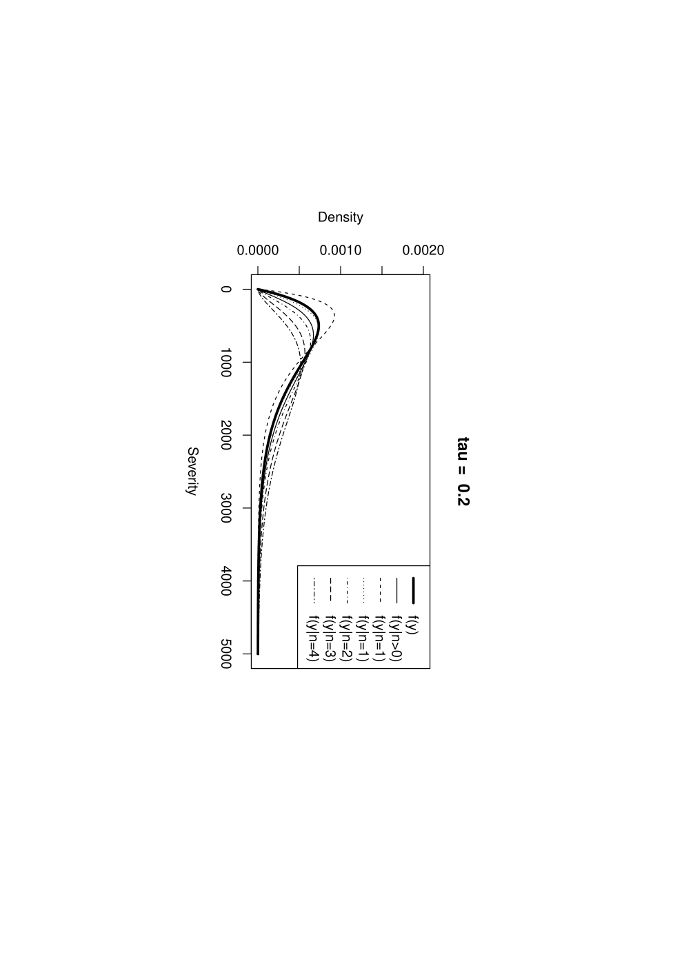
The second experiment examines the effect of frequency-severity dependence on the conditional severity distribution. Figure 2 reports the distribution of given at different levels of dependence. In each panel, we show densities , , and . The former two cases correspond to the common practice where the claim amount is not affected by the number of claims given occurrence. The result is indicative of severe misspecification bias when the dependence between frequency and severity is ignored.



3.2 Estimation based on the Joint Distribution of and
This simulation study examines the finite-sample performance of the estimations based on the joint distribution of and , and further demonstrates the inference bias incurred by ignoring the frequency-severity dependence. We consider the Gaussian copula compound model in a regression context. The primary distribution is Poisson and the secondary distribution is gamma with:
where and are i.i.d. and and . In the Gaussian copula, we consider different degrees of dependence. The copula model is estimated using both the two-stage method and the joint MLE, and the results are summarized in Table 1. We report the relative bias and the root mean squared error. The calculations are based on a sample size of 500 with 250 replications. There is no substantial difference in the estimates from the two approaches. For comparison, we also report in the table the results of the standard two-part model where and are assumed to be independent. As anticipated, the estimates for the frequency model is consistent with the copula approach. However, the estimation assuming conditional independence introduces a long-term bias in the severity model, and this bias positively correlates with the association between and .
Additional simulation studies are provided in Section S.2 of the supplementary material to illustrate the estimation for incomplete data. We emphasize that, in contrast to the cases of complete data and censored data, independence estimation will introduce persistent bias in both frequency and severity components of the model when data are truncated.
| Low Dependence | Independence | Two Stage | Joint MLE | ||||||||
|---|---|---|---|---|---|---|---|---|---|---|---|
| Parameter | Mean | Relative Bias | RMSE | Mean | Relative Bias | RMSE | Mean | Relative Bias | RMSE | ||
| =-1.5 | -1.515 | 0.010 | 0.107 | -1.515 | 0.010 | 0.107 | -1.518 | 0.012 | 0.114 | ||
| = 2.5 | 2.524 | 0.009 | 0.125 | 2.524 | 0.009 | 0.125 | 2.516 | 0.006 | 0.132 | ||
| = 1 | 0.995 | -0.005 | 0.073 | 0.995 | -0.005 | 0.073 | 1.002 | 0.002 | 0.075 | ||
| = 5 | 5.092 | 0.018 | 0.124 | 4.988 | -0.002 | 0.093 | 4.991 | -0.002 | 0.091 | ||
| = -2.5 | -2.552 | 0.021 | 0.110 | -2.493 | -0.003 | 0.101 | -2.495 | -0.002 | 0.105 | ||
| = 5 | 4.977 | -0.005 | 0.056 | 5.004 | 0.001 | 0.054 | 5.001 | 0.000 | 0.051 | ||
| = 2 | 2.061 | 0.030 | 0.109 | 1.998 | -0.001 | 0.097 | 2.005 | 0.003 | 0.093 | ||
| = 0.1 | 0.104 | 0.039 | 0.042 | 0.102 | 0.023 | 0.039 | |||||
| Medium Dependence | Independence | Two Stage | Joint MLE | ||||||||
| Parameter | Mean | Relative Bias | RMSE | Mean | Relative Bias | RMSE | Mean | Relative Bias | RMSE | ||
| = -1.5 | -1.487 | -0.009 | 0.106 | -1.487 | -0.009 | 0.106 | -1.500 | 0.000 | 0.098 | ||
| = 2.5 | 2.478 | -0.009 | 0.118 | 2.478 | -0.009 | 0.118 | 2.501 | 0.000 | 0.116 | ||
| = 1 | 1.005 | 0.005 | 0.078 | 1.005 | 0.005 | 0.078 | 0.998 | -0.002 | 0.069 | ||
| = 5 | 5.419 | 0.084 | 0.429 | 5.002 | 0.000 | 0.082 | 5.002 | 0.000 | 0.079 | ||
| = -2.5 | -2.733 | 0.093 | 0.262 | -2.503 | 0.001 | 0.094 | -2.506 | 0.002 | 0.103 | ||
| = 5 | 4.913 | -0.017 | 0.104 | 5.001 | 0.000 | 0.057 | 5.005 | 0.001 | 0.053 | ||
| = 2 | 2.420 | 0.210 | 0.432 | 2.005 | 0.003 | 0.104 | 2.009 | 0.004 | 0.106 | ||
| = 0.5 | 0.501 | 0.003 | 0.028 | 0.500 | -0.001 | 0.026 | |||||
| High Dependence | Independence | Two Stage | Joint MLE | ||||||||
| Parameter | Mean | Relative Bias | RMSE | Mean | Relative Bias | RMSE | Mean | Relative Bias | RMSE | ||
| =-1.5 | -1.509 | 0.006 | 0.110 | -1.509 | 0.006 | 0.110 | -1.503 | 0.002 | 0.078 | ||
| =2.5 | 2.507 | 0.003 | 0.134 | 2.507 | 0.003 | 0.134 | 2.497 | -0.001 | 0.091 | ||
| = 1 | 1.003 | 0.003 | 0.080 | 1.003 | 0.003 | 0.080 | 1.002 | 0.002 | 0.058 | ||
| = 5 | 5.690 | 0.138 | 0.698 | 4.999 | 0.000 | 0.090 | 5.000 | 0.000 | 0.058 | ||
| = -2.5 | -2.870 | 0.148 | 0.395 | -2.500 | 0.000 | 0.129 | -2.507 | 0.003 | 0.082 | ||
| = 5 | 4.855 | -0.029 | 0.166 | 5.001 | 0.000 | 0.069 | 5.001 | 0.000 | 0.050 | ||
| = 2 | 3.083 | 0.541 | 1.109 | 2.004 | 0.002 | 0.081 | 2.000 | 0.000 | 0.077 | ||
| = 0.9 | 0.900 | 0.000 | 0.006 | 0.901 | 0.001 | 0.006 | |||||
4 Modeling Aggregate Insurance Claims
In nonlife insurance (including property, casualty, and health), the compound distribution (1) is a common approach to modeling aggregate losses in an insurance system. Examples of an insurance system include a single policyholder, a line of business, or a portfolio of contracts. The compound distribution is known as collective risk model in the actuarial literature, and the frequency and severity components are the two building blocks of the model (Klugman et al. 2012).
In this application, we examine the Wisconsin local government property fund which provides property insurance for local government entities in the state of Wisconsin, such as court houses, school districts, fire stations, etc. We consider the building and contents coverage where the building element covers for the physical structure of a property including its permanent fixtures and fittings, and the contents element covers possessions and valuables within the property that are detached and removable. Similar to most nonlife insurance product, the contract provided by the property fund has a one-year term.
The insurance system in this context corresponds to a policyholder, that is a local government entity. The outcome of interest is the aggregate loss for an entity during the policy year, which is determined by both the number and the size of claims. As discussed in Section 1, the collective risk model implies a frequency-severity approach for modeling the aggregate loss for each policyholder, and the current practice relies on the independence assumption between the two building blocks and in the collective risk model.
The purpose of the analysis below is two-folded: first, we provide empirical evidence of significant negative association between the frequency and severity of insurance claims; second, we show that ignoring the frequency-severity dependence could lead to biased decision-making in insurance operations. In the following sections, we use term “independence model” to refer to the standard frequency-severity model that assumes independence between the frequency and severity components, and “copula model” to refer to the proposed copula approach in Section 2.1 that allows for flexible dependence between the frequency and severity components.
Granular insurance claim data are collected for a portfolio of local government entities for years 2009-2011. For each policyholder, one observes the number of claims and the ground-up loss of each claim during each year. We use data of 2009 and 2010 to develop the model, and data of 2011 for model validation. There are 2,080 and 1,017 policy-year observations in the training data and validation data, respectively.
4.1 Exploring Frequency-Severity Association
To explore the relationship between claim frequency and severity, we display in Figure 3 the violin plot of claim size by the number of claims for the portfolio of government entities. To account for exposure, the claim size is normalized by the amount of coverage. First, one observes that given occurrence, the distribution of claim severity correlates with claim frequency. Second, the violin plot suggests a negative relation between claim severity and frequency, i.e. the amount of claims tends to be smaller for policyholders who have more claims.

To further motivate the usage of the proposed copula model, we perform some preliminary analyses to examine the role of frequency-severity dependence in model fitting. Our starting point is the Tweedie model given it is the industry standard in property-casualty insurance for modeling semi-continuous loss cost. Recall that the Tweedie distribution is a Poisson sum of gamma variables where the Poisson and gamma variables are assumed to be independent. To examine the role of dependence, we further allow the Possion and gamma variables in the Tweedie distribution to be correlated. Specifically, we fit a copula model for the aggregate loss where the frequency is a Poisson variable, and the severity is a gamma variable, and their joint distribution is specified by a bivariate Gaussian copula. The association parameter in the Gaussian copula is estimated to be with a standard error of . This result is consistent with the pattern suggested by Figure 3.
To compare the Tweedie and copula models, we present in Figure 4 two goodness-of-fit plots. Denote as the cumulative distribution function (CDF) of aggregate loss. The left figure shows the fitted CDF of the aggregate loss from the two parametric models along with the empirical estimate. Since the plot of CDF emphasizes the center of the distribution, it is not ideal to visualize the effects of extremal large values. To further investigate the tail fit, the right figure plots between the empirical distribution and the two parametric (Tweedie and copula) models. On one hand, both plots indicate that the copula model exhibits superior fit to the Tweedie model, emphasizing the importance of frequency-severity dependence. On the other hand, there is still room for improvement of goodness-of-fit in both the center and the tail of the distribution. This suggests considering more flexible distributions for marginal behavior. To illustrate, we fit another copula model using zero-one inflated negative binomial distribution for claim frequency, the generalized beta of the second kind (GB2) distribution for claim severity, and a Gaussian copula between the two components. The estimated association parameter is with a standard error of . The corresponding goodness-of-fit plots are also shown in Figure 4. As anticipated, refined marginal models improve the fit, especially in the heavy right tail. Overall, the preliminary analyses suggests that there is significant negative dependence between claim frequency and severity, and accounting for such association enhances the goodness-of-fit for the aggregate loss distribution.


4.2 Empirical Analysis
The observation in Section 4.1 motivates us to jointly examine the frequency and severity components in the collective risk model. Differing from the earlier preliminary analysis, first, we explore using more flexible marginal distributions for modeling the number and the size of insurance claims; second, we incorporate covariates to account for observed heterogeneity, and thus the relation between frequency and severity is interpreted as residual dependence; third, we consider various copula that offer different types of dependence in modeling the frequency-severity relationship.
To facilitate model specification, we examine the distributions of both claim frequency and severity, as well as their relationship with available explanatory variables. The insurance database contains policyholder-specific and claim-specific information that one could use to account for the variation in claim frequency and severity. Details of such covariate information are provided in Section S.3 of the supplementary material. For claim frequency, we consider the policy-level characteristics, including entity type (whether a policyholder is a city, county, township, village, or others), alarm credit (whether a policyholder receives a credit for alarm system), the level of deductible, and the amount of coverage. For illustration, we exhibit in Table 2 the empirical distribution of the number of claims per policyholder in the training data. As usually observed in insurance claims data, the majority of policyholders (about 70%) has zero claims over the year. However, this percentage is much smaller than private lines of business such as personal automobile insurance. Another striking feature of claim counts is there is an excess of ones in addition to the zero inflation. We further break down the frequency distribution by entity type, as shown in Table 2 and visualized in Figure 5. The substantial variation suggests that entity type is an important predictor for the claim count.
| Entity Type | |||||||
| Frequency | Overall | City | County | School | Town | Village | Others |
| 0 | 68.08 | 45.67 | 19.67 | 67.11 | 91.95 | 70.33 | 85.45 |
| 1 | 19.38 | 24.00 | 31.15 | 23.36 | 6.90 | 20.75 | 12.27 |
| 2 | 6.54 | 13.33 | 20.49 | 5.26 | 0.86 | 7.05 | 0.91 |
| 3 | 2.12 | 4.67 | 6.56 | 2.63 | 0.00 | 1.04 | 0.45 |
| 4 | 1.49 | 4.00 | 9.84 | 0.66 | 0.00 | 0.62 | 0.00 |
| 5 | 0.67 | 2.33 | 4.10 | 0.16 | 0.29 | 0.00 | 0.00 |
| 1.73 | 6.00 | 8.20 | 0.82 | 0.00 | 0.21 | 0.91 | |
| Obs | 2080 | 300 | 122 | 608 | 348 | 482 | 220 |
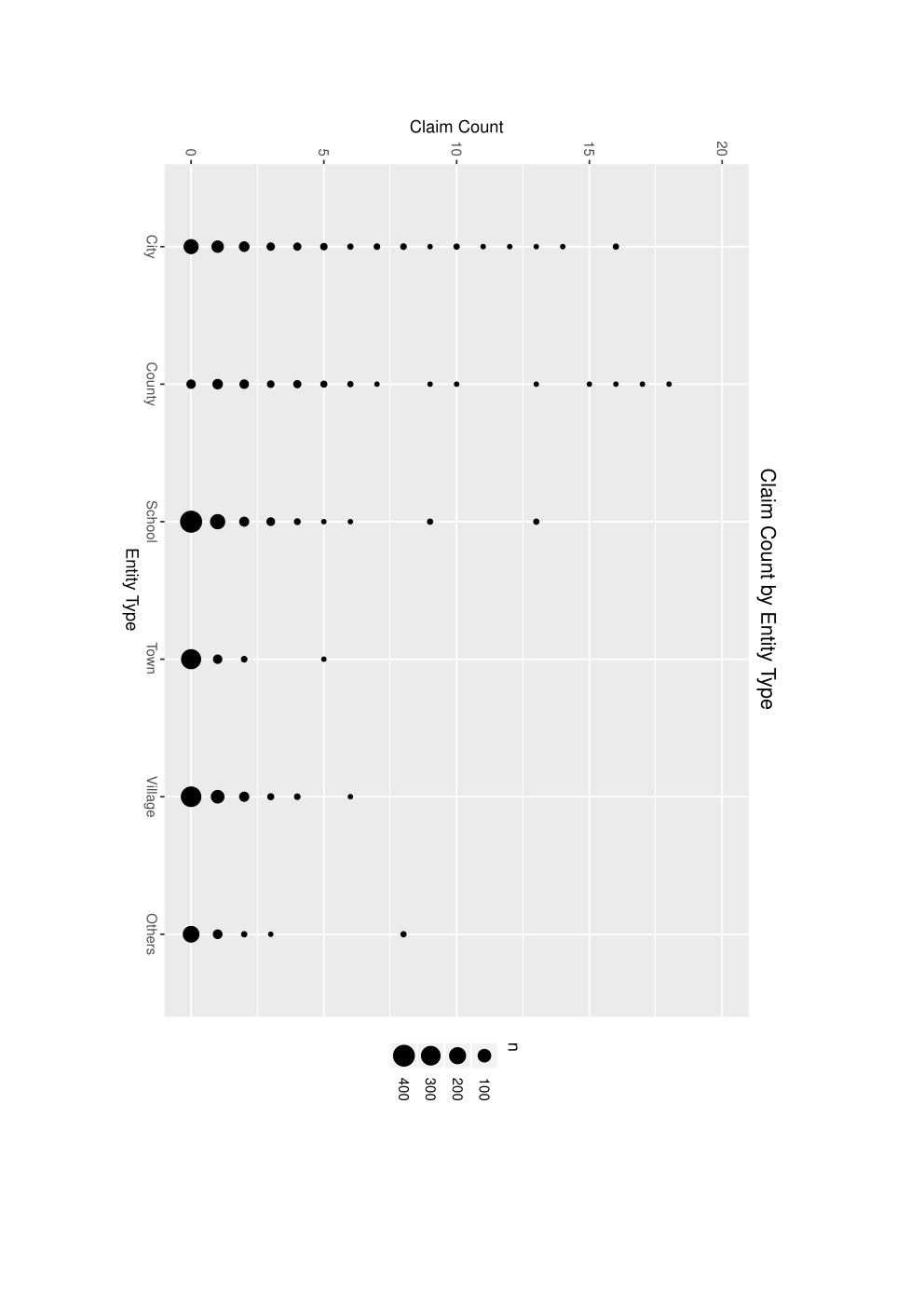
Table 3 summarizes the empirical quantiles of claim amounts. There are in total 1,381 claims in the sampling period. The descriptive statistics indicates that claim amount is skewed and heavy-tailed distributed. For claim severity, besides policy-level information, we look into the effects of claim-level information such as peril type, occurrence time, and reporting delay. As an example, Table 3 shows the empirical distribution of claim amount by peril type and by occurrence time. The claim amount due to fire and water damages tends to be larger compared to other perils, and the loss events occurred in the summer is more likely to result in higher claims. The pattern is also displayed in the violin plot of the claim severity in log scale in Figure 6. The plot reinforces the skewness in the severity distribution and stresses the heterogeneity across occurrence and peril type.


| Peril | Occurrence | ||||||||
| Quantiles | Overall | Fire | Water | Others | Spring | Summer | Fall | Winter | |
| 10 | 946 | 1,072 | 1,009 | 790 | 991 | 950 | 945 | 912 | |
| 25 | 1,645 | 2,168 | 1,641 | 1,418 | 1,600 | 1,655 | 1,746 | 1,666 | |
| 50 | 3,542 | 4,989 | 4,200 | 2,945 | 3,021 | 3,859 | 3,802 | 3,619 | |
| 75 | 9,062 | 13,069 | 11,305 | 5,724 | 7,219 | 11,838 | 8,852 | 7,155 | |
| 90 | 29,288 | 29,849 | 35,640 | 22,203 | 27,872 | 34,181 | 26,890 | 26,758 | |
| Obs | 1381 | 400 | 389 | 592 | 290 | 539 | 289 | 263 | |
In the final model, we consider a zero-one inflated negative binomial regression for claim frequency:
| (12) |
where () is specified using a multinomial logistic regression:
and is a standard negative binomial model:
with being the dispersion parameter. This specification allows to accommodate the excess of both zeros and ones in the claim count. To accommodate the skewness and heavy-tails, a parametric regression based on GB2 distribution is employed for claim severity (for instance, see Shi 2014 for details on GB2 regression):
| (13) |
where and are shape parameters, is the scale parameter, and . A parametric bivariate copula is employed to construct the joint distribution of and . We consider commonly used bivariate copulas from the elliptical and Archimedean families, including Gaussian, , Clayton, Frank, Gumbel, and Joe. For the Archimedean copulas that only allow for positive association, we consider the associated 90 and 270 degree rotated copulas.
The copulas models are estimated using likelihood-based estimation described in Section 2.3. The corresponding goodness-of-fit statistics are reported in Table 4. The independence model is presented as a benchmark. Model selection criteria AIC and BIC recommend the Gaussian copula model. It appears that the tail dependence is not a concern in this context. The implied Kendall’s , reported in the table, reinforces the negative frequency-severity dependence obtained in the earlier analysis, indicating that the claim frequency and severity are correlated after controlling for the covariates. Because the independence model is nested by the copula model, we perform a likelihood ratio test to formally evaluate the goodness-of-fit of the copula models against the independence model. The large statistics confirm the statistical significance of the negative frequency-severity dependence.
The specification for the dependent frequency-severity model, including both the marginals and the copula, is a result of a series of model comparisons, diagnostic analysis, and robust checks. The detailed analysis is provided in Section S.3 of the supplementary material.
| Kendall’s | LogLik | AIC | BIC | Pearson’s | |
|---|---|---|---|---|---|
| Independence | -15,756 | 31,587 | 31,801 | ||
| Gaussian | -0.19 | -15,720 | 31,518 | 31,738 | 70.77 |
| -0.19 | -15,719 | 31,519 | 31,744 | 72.38 | |
| Clayton90 | -0.08 | -15,723 | 31,523 | 31,743 | 66.06 |
| Clayton270 | -0.33 | -15,739 | 31,555 | 31,775 | 34.09 |
| Gumbel90 | -0.29 | -15,722 | 31,521 | 31,741 | 68.04 |
| Gumbel270 | -0.09 | -15,731 | 31,540 | 31,759 | 49.53 |
| Frank90/270 | -0.22 | -15,733 | 31,544 | 31,764 | 45.49 |
| Joe90 | -0.34 | -15,739 | 31,557 | 31,777 | 32.38 |
| Joe270 | -0.05 | -15,735 | 31,548 | 31,768 | 41.41 |
Table 5 reports the estimated parameters for the selected Gaussian copula model. The association parameter in the Gaussian copula is -0.29 and -0.30 using two-stage and full MLE respectively. Given that the rating variables in insurance are highly regulated, one should regard the observed frequency-severity dependence as a result of unobserved heterogeneity, and thus the sign of the dependence could be either positive and negative. Our focus is to provide a data-driven method to capture such relationship and to show the detrimental effects of ignorant supposition of independence on statistical inference and hence insurance operations. For comparison, we also report in Table 5 the estimation results for the independence model. For the frequency component, one anticipates no essential difference in estimates of regression coefficients between the independence and copula models. We observed that the two-stage MLE is identical to the independence model, and we attribute the difference from the full MLE to the finite sample property. In contrast, the difference in the estimates for the severity component is substantial between the independence and copula models (both two-stage and full MLE), which is in line with the significant negative dependence between and . The analysis indicates that ignoring the frequency-severity dependence could introduce significant bias in parameter estimation.
| Independence | Copula-Two Stage MLE | Copula-Full MLE | |||||||||||||||
| Frequency | Severity | Frequency | Severity | Frequency | Severity | ||||||||||||
| Est. | S.E. | Est. | S.E. | Est. | S.E. | Est. | S.E. | Est. | S.E. | Est. | S.E. | ||||||
| Intercept | -1.184 | 0.375 | 7.212 | 0.289 | -1.184 | 0.377 | 7.031 | 0.317 | -0.728 | 0.397 | 6.886 | 0.324 | |||||
| City | 0.299 | 0.257 | -0.333 | 0.198 | 0.299 | 0.244 | -0.548 | 0.216 | 0.485 | 0.232 | -0.616 | 0.216 | |||||
| County | 0.169 | 0.285 | -0.352 | 0.209 | 0.169 | 0.269 | -0.637 | 0.231 | 0.391 | 0.260 | -0.717 | 0.232 | |||||
| School | -0.872 | 0.262 | 0.141 | 0.205 | -0.872 | 0.250 | 0.027 | 0.221 | -0.636 | 0.238 | -0.055 | 0.222 | |||||
| Town | 0.017 | 0.330 | -0.510 | 0.263 | 0.017 | 0.321 | -0.610 | 0.274 | 0.121 | 0.312 | -0.643 | 0.274 | |||||
| Village | 0.247 | 0.253 | -0.180 | 0.200 | 0.247 | 0.243 | -0.387 | 0.215 | 0.383 | 0.235 | -0.434 | 0.215 | |||||
| AlarmCredit05 | 0.328 | 0.216 | 0.060 | 0.201 | 0.328 | 0.215 | 0.024 | 0.201 | 0.316 | 0.212 | 0.026 | 0.200 | |||||
| AlarmCredit10 | 0.316 | 0.205 | -0.121 | 0.177 | 0.316 | 0.203 | -0.201 | 0.181 | 0.356 | 0.201 | -0.217 | 0.180 | |||||
| AlarmCredit15 | 0.227 | 0.136 | -0.115 | 0.121 | 0.227 | 0.135 | -0.123 | 0.124 | 0.290 | 0.134 | -0.147 | 0.124 | |||||
| Deductible | -0.221 | 0.058 | 0.095 | 0.034 | -0.221 | 0.056 | 0.205 | 0.042 | -0.322 | 0.064 | 0.235 | 0.044 | |||||
| Coverage | 0.782 | 0.054 | 0.048 | 0.037 | 0.782 | 0.053 | -0.010 | 0.041 | 0.766 | 0.052 | -0.001 | 0.041 | |||||
| Spring | -0.110 | 0.106 | -0.064 | 0.104 | -0.065 | 0.104 | |||||||||||
| Summer | -0.040 | 0.099 | -0.023 | 0.097 | -0.022 | 0.097 | |||||||||||
| Fall | 0.020 | 0.107 | 0.049 | 0.104 | 0.053 | 0.104 | |||||||||||
| Fire | 0.533 | 0.085 | 0.468 | 0.085 | 0.466 | 0.085 | |||||||||||
| Water | 0.316 | 0.084 | 0.290 | 0.082 | 0.288 | 0.082 | |||||||||||
| ReportDelay | -0.001 | 0.001 | -0.001 | 0.001 | -0.001 | 0.001 | |||||||||||
| Zero-inflated Regression | |||||||||||||||||
| Intercept | -7.834 | 1.406 | -7.834 | 1.476 | -8.583 | 2.126 | |||||||||||
| Deductible | 1.097 | 0.185 | 1.097 | 0.195 | 1.126 | 0.266 | |||||||||||
| Coverage | -0.538 | 0.177 | -0.538 | 0.173 | -0.583 | 0.229 | |||||||||||
| One-inflated Regression | |||||||||||||||||
| Intercept | -7.411 | 1.507 | -7.411 | 1.557 | -7.084 | 1.829 | |||||||||||
| Deductible | 0.664 | 0.217 | 0.664 | 0.224 | 0.577 | 0.266 | |||||||||||
| Coverage | 0.020 | 0.182 | 0.020 | 0.184 | 0.016 | 0.201 | |||||||||||
| -0.290 | 0.034 | -0.303 | 0.033 | ||||||||||||||
4.3 Implications on Insurance Operations
The previous section shows the statistical significance of the dependence between frequency and severity in the collective risk model. This section focuses on the substantive significance of the frequency-severity dependence and demonstrates its impacts on the decision-making in some key insurance operations (Frees 2015).
The first operation that we consider is underwriting and ratemaking. They are two basic functions in insurance companies and are closely related to each other. The former deals with the selection of risks, and latter deals with the determination of the price for the risks accepted. To achieve the underwriting profit target, the central task in underwriting and ratemaking is to quantify the risks of potential customers, which provides the insurer a risk score of policyholders to facilitate portfolio selection. To compare performance of the independence and the copula models, we look to the policyholders in the validation data of 2011 and examine which method leads to a more profitable portfolio construction.
For the purpose of underwriting, we use the coefficient of variation to measure the risk of policyholders. For each of the 1,017 policyholders in year 2011, we calculate the coefficient of variation of the loss cost, denoted for the th policyholder. Given that the aggregate loss cost is specified using a collective risk model (1), the mean and variance of is calculated by:
The above calculation emphasizes the role of the dependency between the two building blocks, frequency and severity. We calculate the distribution of aggregate loss for each policyholder based on 10,000 Monte Carlo simulations. The upper panel of Figure 7 compares the risk ranking between the independence and the copula models. The first plot is the scatter plot of the ranking for each policyholder by the two methods. The second plot shows the realized aggregate losses (in log scale) with the same ranking from the two models. The risk scores from the two models are highly correlated yet there are considerable difference in their rankings.
To evaluate whether the risk ranking points to a profitable portfolio selection strategy, we display in the lower panel of Figure 7 the cumulative loss distribution () versus the cumulative premium distribution (), both ordered by the riskiness of the policyholders . This curve is known as the ordered Lorenz curve in Frees et al. 2011. In Figure 7, the loss and premium distributions are calibrated using the realized losses of the policyholders and the actual premiums charged by the insurer in year 2011, respectively. The area between the curve and the 45 degree line is interpreted as an average profit or loss for the portfolio, with a convex curve for profit and a concave curve for loss. If one thinks of each underwriting strategy as retaining policies with riskiness less than or equal to , the area represents an average profit in the sense that we are taking an expectation over all decision-making strategies. Furthermore, twice the area is known as the Gini index which thus has a natural economic interpretation. The Lorenz curve for the independence model is close to the 45 degree line. In contrast, the Lorenz curve for the copula model suggests a much higher average profit. Specifically, the Gini indices are 10.55% and 33.24% for the independence and the copula models, respectively. Therefore, a better underwriting strategy could be formed using the copula model, given that each policyholder is charged the contract premium.


We next compare the rates suggested by the independence and the copula models. A fair rate commensurate with the policyholder’s risk mitigates adverse selection against the insurer. We perform a out-of-sample validation based on the Gini correlation in Frees et al. 2011. Two base premiums are considered, the constant premium and the contract premium. The former charges average cost to each policyholder, and the latter is the premium that the property fund charges based on the basic rating variables. Table 6 presents the Gini correlation coefficients for the independence and the copula models. For both premium bases, the copula model shows a higher index, implying a more refined risk classification than the independence model.
| Independence | Copula | |
| Constant Premium | 57.61 (6.57) | 63.24 (6.82) |
| Contract Premium | 15.93 (8.81) | 26.27 (11.15) |
| † Standard errors are reported in parentheses. | ||
The proposed copula model can also provide insights for the practice of claims reserving. In property casualty insurance, it is typical that a loss event won’t be reported to the insurer immediately upon occurrence. For instance, a hail damage to the roof might be discovered by the policyholder several month later. After being reported, it further takes time for the insurer to decide coverage and finally settle the claim. Because of the long reporting and settlement delays, an insurer could be responsible for future payments associated with the loss events occurred in the policy period even post the expiration of the contract. Claims reserving or loss reserving is the process of estimating outstanding payments or the ultimate payments that an insurer is responsible for. Reserves are determined at both claim level and portfolio level (see, for example, Antonio and Beirlant 2008 and Pigeon et al. 2014). At claim level, an insurer estimates the amount for which a particular claim will ultimately be settled or adjudicated, also known as case reserve. At portfolio level, an insurer also estimates its future liabilities for the entire book of business. To emphasize its importance, loss reserves typically represent the largest liability item on the balance sheet of nonlife insurers.
For reserving purposes, one is interested in the claims amount given occurrence of the loss events. As pointed out by Wüthrich and Merz 2008, because of the introduction of new supervisory guidelines (Solvency II) and financial reporting standards (IFRS 4 Phase II), the measurement of future cash flows and their uncertainty becomes more important. In this application, we examine the predictive distribution of given . For illustration, we display in Figure 8 the 95% prediction intervals of the claims amount for four representative risks, “poor”, “good”, “average”, and “superior”. The bar is determined by the 2.5th and 97.5th percentiles of the predictive distribution, and the solid dot indicates the predictive mean. The four risks are selected from the validation data based on the expected number of claims . Specifically, they expect to have 2.37, 0.76, 0.37, 0.15 claims per year which corresponding to the 95th, 75th, 50th, 25th percentiles of the frequency distribution, respectively. For comparison, we impose the corresponding prediction interval from the independence model in the figure as indicated by the dashed line. First, as expected, the predictive distribution of claim amounts given frequency is skewed and long-tailed. This observation emphasizes that a range estimate of reserves is more informative than a point estimate for managers to set appropriate reserves, because an insurer doesn’t want to overestimate nor underestimate its outstanding liabilities. Over-reserving could inflate the price and make the product less competitive, while under-reserving increases the solvency risk. Second, because of the significant negative relation between claim frequency and severity, the claims amount becomes smaller as the number of claims increases. A dynamic viewpoint is that an insurer updates its knowledge on the severity distribution based on frequency information. Third, it is apparent that ignoring the frequency-severity dependence will introduce significant bias in the reserving estimates. Under the independence assumption, not only that the claim severity is invariant with respect to claim frequency, but also the magnitude of the prediction could lead to poor decision making. For example, the results suggest that managers relying on the independence model tend to over reserve for better risks. In particular, the over-reserving risk is substantial for superior risks. As described earlier, there will be negative effects on both pricing and reserving. Over prediction of unpaid losses lead to increase in price which could cause the insurer to lose profitable business.


We further test the prediction of ultimate losses given occurrence for all the policyholders in the hold-out sample. To compare the prediction from the independence model to the copula model, we employ the continuous ranked probability score (CRPS) in Gneiting and Raftery 2007 and Czado et al. 2009. The CRPS is a proper scoring rule that assesses the quality of probabilistic forecasts. For reserving purpose, we focus on policyholders with at least one claims, and we evaluate the prediction of the aggregate loss distribution . The predictive distribution is derived for each policyholder based on 10,000 Monte Carlo simulations where the aggregated loss is generated conditional on occurrence of claims. Then the CRPS assigns a numerical score that measures the distance between the cumulative predictive distribution and the realized losses in the hold-out sample. For 73.34% of the policies in the hold-out sample, the copula model outperforms the independence model. A binomial test suggest the superior prediction of the copula model to the independence model is statistically significant.
In the third application, we briefly demonstrate implications of the frequency-severity dependence on capital management. Insurance is a highly regulated industry. To mitigate solvency risk and protect public interest, insurers are required to hold minimum amount of risk capital as a buffer in case of some unexpected catastrophic events. We have already seen the consequences when the dependence between frequency and severity is unaccounted for at the individual policy level. This example emphasizes its relevance at the portfolio level since the risk capital is determined for the entire book of business.
To calculate the risk capital, we consider the value-at-risk (VaR), a risk measure widely used in the insurance and banking industry. The VaR focuses on the tail of the distribution, and specifically VaR is defined as the th percentile. Our interest is the aggregate losses for the insurance portfolio, defined as , where , the loss cost for policyholder , is specified using the collective risk model (1). The distribution of is estimated using 10,000 Monte Carlo simulations. Table 7 reports the risk measure at 90%, 95%, and 99% levels for both the independence and copula models. To quantify the simulation uncertainty, we replicate the simulation 100 times to obtain the 95% confidence interval. The results implies that ignoring the frequency-severity dependence in the collective risk model leads to significant underestimate of the tail risk for the portfolio.
| 0.90 | 0.95 | 0.99 | |
|---|---|---|---|
| Independence | 39,556 | 69,124 | 314,854 |
| (38,961, 40,162) | (67,834, 70,521) | (300,348, 328,009) | |
| Copula | 41,665 | 75,114 | 374,234 |
| (41,106,42,210) | (73,921,76,284) | (349,748, 397,509) | |
| Difference | 5.33% | 8.67% | 18.86% |
5 Conclusion
The two-part regression model based on compound distributions is commonly used in various disciplines, including insurance, economics, marketing, and psychology, among others. The current practice is to perform a marginal regression on the primary (frequency) outcome, and a separate regression on the positive portion of the secondary (severity) outcome. This practice relies on the (conditional) independence assumption and causes significant biases in inference in the presence of frequency-severity dependence.
Motivated by the wide application of this type of model, this article represents the first attempt at accommodating the association between the frequency and severity components in the compound distribution and the associated regression models. We proposed the novel idea of using a parametric copula to construct the joint distribution of and in the compound distribution. The copula regression is simple yet enjoys several advantages: First, the copula model allows for an arbitrary dependence between frequency and severity, and thus includes the (conditional) independence model as a special case. Second, separating the marginal from the joint distribution, the copula model can easily accommodate nonstandard marginal regressions for complicated data structure, for instance, regressions for zero/one-inflated data or the incomplete data due to censoring and truncation. Third, the parametric nature of the model implies straightforward likelihood-based inference and thus facilitates data-driven model specification and diagnostics, which is critical to the applications with complex and big data.
This work was motivated by the applications in insurance, where the complex and unique features of claims data provide a general setting to investigate the frequency-severity dependence in the context of the two-part model. For example, the standard count regression is not sufficient to capture the features in claim frequency; and the modifications on insurance coverage often cause observations to be incomplete. Although our empirical analysis emphasized the consequences of ignoring the frequency-severity dependence on the operations in insurance companies, the proposed model is general enough and ready to apply to other disciplines. It’ll be interesting to see the implications of the frequency-severity dependence on decision making in other fields as well.
Finally, we conclude the paper with some discussions on the dependence between the frequency and severity in the proposed copula model. First, the proposed copula model relies on a simplifying assumption for the dependence, i.e. the association parameter in the copula is constant and does not vary across covariates. A potential extension is to use a conditional copula approach to allow the association in the copula to be dependent on covariates. See, for example, Patton 2006, Acar et al. 2011, Veraverbeke et al. 2011, Fermanian and Wegkamp 2012, and Castro-Camilo et al. 2018 for some recent development. We note that some domain knowledge is usually needed to support the conditional copula approach, for instance, the dependence among stock markets could be time-varying. We leave it as a future research topic to investigate the conditional dependence in insurance data. Second, we attribute the observed dependence in frequency and severity to unobserved heterogeneity. Regarding whether such relation is positive or negative, we think of this more as an empirical question to investigate. Often there are competing theories to support both positive and negative relationships. For the property insurance in our paper, one example of unobserved heterogeneity that induces dependence is weather related hazard. One can think of a geographical region that has frequent but modest storms versus another region that has infrequent but very severe storms. Another example of unobserved heterogeneity is the social-economic factors. One can think of some areas with frequent but minor crimes versus other areas with infrequent but severe crimes. Thus it is important for the model to offer the flexibility to accommodate both positive and negative relationship, and thus to allow for an empirical test of alternative theories.
SUPPLEMENTARY MATERIAL
S.1 Special Cases of the Copula Models
We show that several widely used two-part models can be viewed in the proposed copula framework. The first is the hurdle model in the health economics literature (see, for instance, Mullahy 1986 and Pohlmeier and Ulrich 1995). The hurdle model considers the count measure of health care utilisation as a result of two different decision processes. The first part specifies the decision to seek care by individuals, and the second decision concerns the quantity of health care consumed which is partly determined by physicians. In the copula model, define and for a latent count variable . The copula for and is shown to be . In this case, the copula model (4) becomes:
| (S.1) |
This gives the standard hurdle model where the hurdle component can be a logit or a probit regression, and the truncated component is usually a Poisson or a negative binomial model. Governed by two different sets of parameters, the two components are separately and independently estimated. The same framework has also been used to study the semi-continuous health care expenditures where a log-linear or generalized linear model is often employed for the truncated component (see Mullahy 1998).
The second special case is the selection model. Assuming is a binary outcome and is determined by a latent continuous variable through relation , one has:
Denote as the copula that uniquely defines the joint distribution of and , the bivariate density of and can be expressed as:
where . Then the distribution of and is:
Note that the above is a selection model in that is observed only if . See Smith 2003 and Prieger 2002 for discussions on copula-based selection model. When and are joint normal distribution, the copula model further reduces to the classic Heckman model (Heckman 1979).
Under this setting, the joint distribution of is shown:
The model has a natural two-part interpretation where the joint distribution decouples into the product of frequency and severity distributions. However, the two components cannot be estimated separately because they are not independent with each other.
The last related case is the frequency-severity model in the actuarial science literature (Frees 2014), where the joint distribution of is expressed as:
| (S.2) |
The frequency component describes the number of claims and is specified as a count regression. The severity component governs the size of claims given occurrence and employs generalized linear models to account for the skewness and heavy tails. The model assumes that given , the distribution of does not depend on . Thus the two pieces can be estimated separately. Note the difference between distributions and . To be more specific,
The frequency-severity model can also be formulated using the proposed copula framework. Consider the case where and is only related through the relation between , which is defined as , and . That is, and are independent conditional on . Let denote the copula that defines the joint distribution of and , we have
Then the joint distribution of and can be shown as:
| (S.3) |
Using (S.1 Special Cases of the Copula Models), the copula model (4) becomes the standard frequency-severity model (S.2), which further reduces to (9) when and are independent. It is important to note that models (9) and (S.2) are indistinguishable because is not completely observed and thus only the partial information corresponding to is available for inference.
S.2 Additional Simulation Studies
In this section, we conduct additional simulation studies to examine the estimation performance for censored and truncated data as described in Section 2.2. We set the deductible and policy limit , which are roughly the 20th and 90th percentiles of the marginal distribution of . Estimation results using independence estimation and joint MLE are summarized in Table S.1 and Table S.2 for the censored and truncated data respectively. In general, the joint MLE performs well for both cases of incomplete data. Higher estimation uncertainty is associated with the truncated data compared to the censored data due to less amount of information available. The comparison with independence estimation emphasizes the significant bias when ignoring the dependence between frequency and severity. Similar to the complete data, when data are censored, independence estimation only introduces persistent bias in the severity model while the frequency model can still be consistently estimated. However, large bias is anticipated and observed in both frequency and severity models when data are truncated, and the bias won’t disappear when sample size increases.
| Independence | Joint MLE | ||||||
|---|---|---|---|---|---|---|---|
| Low Dependence | Mean | Relative Bias | RMSE | Mean | Relative Bias | RMSE | |
| =-1.5 | -1.508 | 0.005 | 0.116 | -1.504 | 0.003 | 0.111 | |
| = 2.5 | 2.513 | 0.005 | 0.144 | 2.507 | 0.003 | 0.140 | |
| = 1 | 0.998 | -0.002 | 0.073 | 0.997 | -0.003 | 0.071 | |
| = 5 | 5.084 | 0.017 | 0.115 | 4.997 | -0.001 | 0.093 | |
| = -2.5 | -2.561 | 0.025 | 0.139 | -2.499 | -0.000 | 0.121 | |
| = 5 | 4.998 | -0.000 | 0.077 | 5.005 | 0.001 | 0.070 | |
| = 2 | 2.064 | 0.032 | 0.127 | 2.015 | 0.008 | 0.113 | |
| = 0.1 | 0.097 | -0.030 | 0.042 | ||||
| Medium Dependence | Mean | Relative Bias | RMSE | Mean | Relative Bias | RMSE | |
| =-1.5 | -1.508 | 0.005 | 0.116 | -1.505 | 0.004 | 0.106 | |
| = 2.5 | 2.513 | 0.005 | 0.144 | 2.507 | 0.003 | 0.131 | |
| = 1 | 0.998 | -0.002 | 0.073 | 0.998 | -0.002 | 0.070 | |
| = 5 | 5.421 | 0.084 | 0.432 | 4.996 | -0.001 | 0.089 | |
| = -2.5 | -2.762 | 0.105 | 0.300 | -2.495 | -0.002 | 0.128 | |
| = 5 | 4.940 | -0.012 | 0.097 | 5.002 | 0.000 | 0.064 | |
| = 2 | 2.370 | 0.185 | 0.393 | 2.019 | 0.010 | 0.127 | |
| = 0.5 | 0.499 | -0.002 | 0.030 | ||||
| High Dependence | Mean | Relative Bias | RMSE | Mean | Relative Bias | RMSE | |
| =-1.5 | -1.508 | 0.005 | 0.116 | -1.506 | 0.004 | 0.083 | |
| = 2.5 | 2.513 | 0.005 | 0.144 | 2.508 | 0.003 | 0.097 | |
| = 1 | 0.998 | -0.002 | 0.073 | 1.000 | 0.000 | 0.066 | |
| = 5 | 5.727 | 0.145 | 0.737 | 4.995 | -0.001 | 0.070 | |
| = -2.5 | -2.952 | 0.181 | 0.492 | -2.491 | -0.004 | 0.117 | |
| = 5 | 4.894 | -0.021 | 0.153 | 4.999 | -0.000 | 0.056 | |
| = 2 | 2.945 | 0.473 | 0.985 | 2.013 | 0.007 | 0.095 | |
| = 0.9 | 0.900 | 0.000 | 0.006 | ||||
| Independence | Joint MLE | ||||||
|---|---|---|---|---|---|---|---|
| Low Dependence | Mean | Relative Bias | RMSE | Mean | Relative Bias | RMSE | |
| =-1.5 | -1.512 | 0.008 | 0.190 | -1.508 | 0.005 | 0.183 | |
| = 2.5 | 2.507 | 0.003 | 0.156 | 2.494 | -0.002 | 0.151 | |
| = 1 | 1.001 | 0.001 | 0.198 | 0.997 | -0.003 | 0.191 | |
| = 5 | 5.085 | 0.017 | 0.137 | 5.004 | 0.001 | 0.117 | |
| = -2.5 | -2.562 | 0.025 | 0.139 | -2.501 | 0.000 | 0.124 | |
| = 5 | 4.997 | -0.001 | 0.097 | 4.998 | -0.000 | 0.090 | |
| = 2 | 2.067 | 0.034 | 0.137 | 2.019 | 0.010 | 0.118 | |
| = 0.1 | 0.097 | -0.031 | 0.045 | ||||
| Medium Dependence | Mean | Relative Bias | RMSE | Mean | Relative Bias | RMSE | |
| =-1.5 | -1.440 | -0.040 | 0.172 | -1.500 | -0.000 | 0.153 | |
| = 2.5 | 2.515 | 0.006 | 0.154 | 2.500 | -0.000 | 0.137 | |
| = 1 | 0.929 | -0.071 | 0.185 | 0.987 | -0.013 | 0.152 | |
| = 5 | 5.384 | 0.077 | 0.401 | 4.997 | -0.001 | 0.096 | |
| = -2.5 | -2.753 | 0.101 | 0.291 | -2.500 | -0.000 | 0.132 | |
| = 5 | 4.971 | -0.006 | 0.097 | 5.001 | 0.000 | 0.073 | |
| = 2 | 2.345 | 0.172 | 0.371 | 2.017 | 0.008 | 0.130 | |
| = 0.5 | 0.499 | -0.003 | 0.033 | ||||
| High Dependence | Mean | Relative Bias | RMSE | Mean | Relative Bias | RMSE | |
| =-1.5 | -1.403 | -0.065 | 0.172 | -1.508 | 0.005 | 0.115 | |
| = 2.5 | 2.521 | 0.008 | 0.148 | 2.499 | -0.000 | 0.108 | |
| = 1 | 0.888 | -0.112 | 0.190 | 1.002 | 0.002 | 0.114 | |
| = 5 | 5.671 | 0.134 | 0.685 | 4.996 | -0.001 | 0.076 | |
| = -2.5 | -2.941 | 0.177 | 0.485 | -2.499 | -0.000 | 0.135 | |
| = 5 | 4.946 | -0.011 | 0.148 | 5.001 | 0.000 | 0.068 | |
| = 2 | 2.863 | 0.432 | 0.906 | 2.013 | 0.007 | 0.098 | |
| = 0.9 | 0.900 | -0.001 | 0.007 | ||||
S.3 Covariates, Diagnostic Analysis, and Robustness Check
Table S.3 summarizes the covariates (both variable description and descriptive statistics) in the regression analysis. The frequency model uses the policy-specific covariates only, the severity model uses both policy-specific and claim-specific covariates.
| Variable | Description | Mean | SD |
| Policy-specific | |||
| City | Indicator of city | 0.144 | |
| County | Indicator of county | 0.059 | |
| School | Indicator of school | 0.292 | |
| Town | Indicator of town | 0.167 | |
| Village | Indicator of village | 0.232 | |
| Misc | Indicator of miscellaneous entities (example: fire station) | 0.106 | |
| AlarmCredit00 | Indicator of 0% alarm credit | 0.346 | |
| AlarmCredit05 | Indicator of 5% alarm credit | 0.064 | |
| AlarmCredit10 | Indicator of 10% alarm credit | 0.076 | |
| AlarmCredit15 | Indicator of 15% alarm credit | 0.513 | |
| Deductible | Log of deductible amount in dollars | 7.208 | 1.174 |
| Coverage | Log of coverage amount in millions of dollars | 2.261 | 1.976 |
| Claim-specific | |||
| Spring | Indicator of whether occurrence in spring | 0.211 | |
| Summer | Indicator of whether occurrence in summer | 0.391 | |
| Fall | Indicator of whether occurrence in fall | 0.208 | |
| Winter | Indicator of whether occurrence in winter | 0.190 | |
| Fire | Indicator of fire peril of loss | 0.290 | |
| Water | Indicator of water peril of loss | 0.281 | |
| Other | Indicator of other perils of loss | 0.429 | |
| ReportDelay | Log of delay in accident report in days | 2.725 | 1.369 |
We follow the procedures described in Section 2.3 to perform diagnostic checking. For the frequency model, we investigate the popular Poisson and negative binomial regressions, along with their zero inflated and zero-one inflated versions. Table S.4 presents the goodness-of-fit statistics for the alternative count regressions. The poor fit of the Poisson model is not surprising due to its incapability to handle zero-inflation and over dispersion. The negative binomial regression and the zero-inflated models account for zero inflation but do not accommodate the probability mass at one. The Pearson’s statistic is in favor of the zero-one inflated negative binomial model.
| Empirical | Poisson | NB | ZIP | ZINB | ZOIP | ZOINB | |
|---|---|---|---|---|---|---|---|
| % of zeros | 0.681 | 0.643 | 0.688 | 0.678 | 0.689 | 0.679 | 0.683 |
| % of ones | 0.194 | 0.211 | 0.178 | 0.173 | 0.176 | 0.196 | 0.195 |
| -stat | 111.73 | 38.67 | 97.33 | 41.09 | 40.41 | 32.13 |
As discussed in Section 2.3, the marginal distribution of and the copula cannot be separately identified. Therefore, the model checking is based on the conditional distribution . Figure S.1 displays the QQ plot of the normal scores and the histogram of the Cox-Snell residuals . There is no irregular pattern in the plots, suggesting that the severity distribution and the bivariate copula are well specified. The slight deviation in the left tail of the QQ plot is caused by five claims that have one dollar as claim amount, which bear minimal impact in insurance operation. A formal uniform test for the Cox-Snell residuals is provided in Table S.5, and the large -values support the uniformity of the residuals.


| Statistics | -value | |
|---|---|---|
| Kolmogorov-Smirnov | 0.020 | 0.613 |
| Cramer-von Mises | 0.085 | 0.665 |
| Anderson-Darling | 0.943 | 0.388 |
In the analysis of Wisconsin property fund data, we have found significant negative association between the number of claims and the size of claims for local government entities. One question of interest is how robust this negative relationship is with respect to the year of observations. Recall that we have used data of 2009 and 2010 to build the model and reserved the data of 2011 for hold-out sample validation. For the purpose of robustness check, we reestimate the proposed copula model with all three years of data. To focus on the frequency-severity dependence, we consider the same set of copula candidates as in Table 4. The results are summarized in Table S.6. First, the magnitude and the statistical significance of the negative association is in line with the estimates in Table 4. Second, the same favorite, Gaussian copula, is selected by the information criteria and goodness-of-fit statistic.
| Kendall’s | LogLik | AIC | BIC | Pearson’s | |
|---|---|---|---|---|---|
| Independence | -23,722 | 47,522 | 47,769 | ||
| Gaussian | -0.20 | -23,667 | 47,412 | 47,659 | 110.20 |
| -0.20 | -23,667 | 47,412 | 47,659 | 110.20 | |
| Clayton90 | -0.08 | -23,678 | 47,434 | 47,682 | 87.82 |
| Clayton270 | -0.35 | -23,689 | 47,456 | 47,703 | 66.18 |
| Gumbel90 | -0.29 | -23,671 | 47,419 | 47,666 | 103.06 |
| Gumbel270 | -0.08 | -23,692 | 47,462 | 47,709 | 60.24 |
| Frank90/270 | -0.23 | -23,683 | 47,444 | 47,691 | 78.14 |
| Joe90 | -0.37 | -23,692 | 47,461 | 47,708 | 61.06 |
| Joe270 | -0.04 | -23,698 | 47,475 | 47,722 | 47.26 |
References
- Acar et al. (2011) Acar, E. F., R. V. Craiu, and F. Yao (2011). Dependence calibration in conditional copulas: A nonparametric approach. Biometrics 67(2), 445–453.
- Albrecher et al. (2017) Albrecher, H., J. L. Teugels, and J. Beirlant (2017). Reinsurance: Actuarial and Statistical Aspects. John Wiley & Sons.
- Antonio and Beirlant (2008) Antonio, K. and J. Beirlant (2008). Issues in claims reserving and credibility: a semiparametric approach with mixed models. Journal of Risk and Insurance 75(3), 643–676.
- Aribarg et al. (2010) Aribarg, A., R. Pieters, and M. Wedel (2010). Raising the bar: Bias adjustment of recognition tests in advertising. Journal of Marketing Research 47(3), 387–400.
- Castro-Camilo et al. (2018) Castro-Camilo, D., M. de Carvalho, J. Wadsworth, et al. (2018). Time-varying extreme value dependence with application to leading european stock markets. The Annals of Applied Statistics 12(1), 283–309.
- Czado et al. (2009) Czado, C., T. Gneiting, and L. Held (2009). Predictive model assessment for count data. Biometrics 65(4), 1254–1261.
- Czado et al. (2012) Czado, C., R. Kastenmeier, E. C. Brechmann, and A. Min (2012). A mixed copula model for insurance claims and claim sizes. Scandinavian Actuarial Journal 2012(4), 278–305.
- Fermanian and Wegkamp (2012) Fermanian, J.-D. and M. H. Wegkamp (2012). Time-dependent copulas. Journal of Multivariate Analysis 110, 19–29.
- Frees (2014) Frees, E. (2014). Frequency and severity models. In E. Frees, G. Meyers, and R. A. Derrig (Eds.), Predictive Modeling Applications in Actuarial Science, Volume I: Predictive Modeling Techniques, Cambridge, pp. 138–166. Cambridge University Press.
- Frees (2015) Frees, E. W. (2015). Analytics of insurance markets. Annual Review of Financial Economics 7, 253–277.
- Frees et al. (2011) Frees, E. W., J. Gao, and M. A. Rosenberg (2011). Predicting the frequency and amount of health care expenditures. North American Actuarial Journal 15(3), 377–392.
- Frees et al. (2016) Frees, E. W., G. Lee, and L. Yang (2016). Multivariate frequency-severity regression models in insurance. Risks 4(1), 4.
- Frees et al. (2011) Frees, E. W., G. Meyers, and A. D. Cummings (2011). Summarizing insurance scores using a gini index. Journal of the American Statistical Association 106(495), 1085–1098.
- Garrido et al. (2016) Garrido, J., C. Genest, and J. Schulz (2016). Generalized linear models for dependent frequency and severity of insurance claims. Insurance: Mathematics and Economics 70, 205–215.
- Gneiting and Raftery (2007) Gneiting, T. and A. E. Raftery (2007). Strictly proper scoring rules, prediction, and estimation. Journal of the American Statistical Association 102(477), 359–378.
- Heckman (1979) Heckman, J. J. (1979). Sample selection bias as a specification error. Econometrica 47(1), 153–161.
- Joe (2005) Joe, H. (2005). Asymptotic efficiency of the two-stage estimation method for copula-based models. Journal of Multivariate Analysis 94(2), 401–419.
- Joe (2014) Joe, H. (2014). Dependence Modeling Using Copulas. Chapman & Hall.
- Johnson et al. (2005) Johnson, N. L., A. W. Kemp, and S. Kotz (2005). Univariate discrete distributions (3 ed.). New Jersey: John Wiley & Sons.
- Jorgensen (1987) Jorgensen, B. (1987). Exponential dispersion models. Journal of the Royal Statistical Society. Series B (Methodological) 49(2), 127–162.
- Jørgensen and de Souza (1994) Jørgensen, B. and M. de Souza (1994). Fitting Tweedie’s compound poisson model to insurance claims data. Scandinavian Actuarial Journal 1(1), 69–93.
- Karlis and Xekalaki (2005) Karlis, D. and E. Xekalaki (2005). Mixed poisson distributions. International Statistical Review 73(1), 35–58.
- Klugman et al. (2012) Klugman, S. A., H. H. Panjer, and G. E. Willmot (2012). Loss Models: from Data to Decisions (4th ed.). John Wiley & Sons.
- Krämer et al. (2013) Krämer, N., E. C. Brechmann, D. Silvestrini, and C. Czado (2013). Total loss estimation using copula-based regression models. Insurance: Mathematics and Economics 53(3), 829–839.
- Lin (2014) Lin, X. (2014). Compound distributions. Wiley StatsRef: Statistics Reference Online, doi: 10.1002/9781118445112.stat04411.
- Liu and Wang (2017) Liu, H. and R. Wang (2017). Collective risk models with dependence uncertainty. ASTIN Bulletin: The Journal of the IAA 47(2), 361–389.
- Mullahy (1986) Mullahy, J. (1986). Specification and testing of some modified count data models. Journal of econometrics 33(3), 341–365.
- Mullahy (1998) Mullahy, J. (1998). Much ado about two: reconsidering retransformation and the two-part model in health econometrics. Journal of health economics 17(3), 247–281.
- Nelsen (2006) Nelsen, R. (2006). An Introduction to Copulas. Springer.
- Newey and McFadden (1994) Newey, W. K. and D. McFadden (1994). Large sample estimation and hypothesis testing. Handbook of econometrics 4, 2111–2245.
- Olsen and Schafer (2001) Olsen, M. K. and J. L. Schafer (2001). A two-part random-effects model for semicontinuous longitudinal data. Journal of the American Statistical Association 96(454), 730–745.
- Panjer (2006) Panjer, H. H. (2006). Operational risk: modeling analytics, Volume 620. John Wiley & Sons.
- Patton (2006) Patton, A. J. (2006). Modelling asymmetric exchange rate dependence. International economic review 47(2), 527–556.
- Pigeon et al. (2014) Pigeon, M., K. Antonio, and M. Denuit (2014). Individual loss reserving using paid–incurred data. Insurance: Mathematics and Economics 58, 121–131.
- Pohlmeier and Ulrich (1995) Pohlmeier, W. and V. Ulrich (1995). An econometric model of the two-part decisionmaking process in the demand for health care. Journal of Human Resources, 339–361.
- Prieger (2002) Prieger, J. E. (2002). A flexible parametric selection model for non-normal data with application to health care usage. Journal of Applied Econometrics 17(4), 367–392.
- Shevchenko (2010) Shevchenko, P. V. (2010). Calculation of aggregate loss distributions. The Journal of Operational Risk 5(2), 3.
- Shi (2014) Shi, P. (2014). Fat-tailed regression models. In E. Edward, G. Meyers, and R. A. Derrig (Eds.), Predictive Modeling Applications in Actuarial Science, Cambridge. Cambridge University Press.
- Shi et al. (2016) Shi, P., X. Feng, J.-P. Boucher, et al. (2016). Multilevel modeling of insurance claims using copulas. The Annals of Applied Statistics 10(2), 834–863.
- Shi and Yang (2018) Shi, P. and L. Yang (2018). Pair copula constructions for insurance experience rating. Journal of the American Statistical Association 113(521), 122–133.
- Silva and Windmeijer (2001) Silva, J. M. S. and F. Windmeijer (2001). Two-part multiple spell models for health care demand. Journal of Econometrics 104(1), 67–89.
- Smith (2003) Smith, M. D. (2003). Modelling sample selection using archimedean copulas. The Econometrics Journal 6(1), 99–123.
- Smithson and Shou (2014) Smithson, M. and Y. Shou (2014). Randomly stopped sums: models and psychological applications. Frontiers in psychology 5, 1–11.
- Smyth and Jørgensen (2002) Smyth, G. and B. Jørgensen (2002). Fitting Tweedie’s compound poisson model to insurance claims data: dispersion modelling. ASTIN Bulletin 32(1), 143–157.
- Tellis (1988) Tellis, G. J. (1988). Advertising exposure, loyalty, and brand purchase: A two-stage model of choice. Journal of Marketing Research 25(2), 134–144.
- Tweedie (1984) Tweedie, M. (1984). An index which distinguishes between some important exponential families. In J. Ghosh and J. Roy (Eds.), Statistics: Applications and New Directions. Proceedings of the Indian Statistical Institute Golden Jubilee International Conference, pp. 579–604. Indian Statistical Institute, Calcutta.
- Veraverbeke et al. (2011) Veraverbeke, N., M. Omelka, and I. Gijbels (2011). Estimation of a conditional copula and association measures. Scandinavian Journal of Statistics 38(4), 766–780.
- Wüthrich and Merz (2008) Wüthrich, M. V. and M. Merz (2008). Stochastic claims reserving methods in insurance, Volume 435. John Wiley & Sons.