Optimal stopping contract for Public Private Partnerships under moral hazard

Ishak Hajjej Thanks: CREST $&$ ENSIIE, LaMME, France, email ishak.hajjej@ensae.fr Caroline Hillairet Thanks: CREST, ENSAE Paris, France, email Caroline.Hillairet@ensae.fr Mohamed Mnif Thanks: ENIT, LAMSIN, University of Tunis El Manar, Tunis, Tunisia, email mohamed.mnif@enit.rnu.tn

Abstract

This paper studies optimal Public Private Partnerships contracts between a public entity and a consortium, in continuous-time and with a continuous payment, and the possibility for the public to stop the contract. The public ("she") pays a continuous rent to the consortium ("he"), while the latter gives a best response characterized by his effort. This effort impacts the drift of the social welfare, until a terminal date decided by the public when she stops the contract and gives compensation to the consortium. Usually, the public cannot observe the effort done by the consortium, leading to a principal agent’s problem with moral hazard. Therefore this paper formalizes such PPP contracts into a contract theory problem. Due to the long-term characteristic of PPP contracts, the public should incentivize the consortium to provide effort not only through the terminal payment but also through the rent paid until the end of the contract. We solve this optimal stochastic control with optimal stopping problem in this context of moral hazard. The public value function is characterized by the solution of an associated Hamilton Jacobi Bellman Variational Inequality. The public value function, the optimal effort and rent processes are computed numerically by using the Howard algorithm. In particular, the impact of the social welfare’s volatility on the optimal contract is studied.

Keywords: Moral Hazard, Public Private Partnership, stochastic control, optimal stopping, Hamilton Jacobi Bellman Variational Inequality, Howard algorithm.

MSC Classification : 60G40, 91B40, 91B70, 93E40.

Funding: This research is supported by a grant of the French National Research Agency (ANR), ”Investissements d’Avenir” (LabEx Ecodec/ANR-11-LABX-0047).

Acknowledgments: The authors thank Nizar Touzi, Said Hamaène , Monique Pontier, Alexandre Popier and anonymous referees for fruitful discussions and constructive suggestions.

1 Introduction

Public-private partnership (PPP) is defined as a long-term contract between a private party and a public entity, for the construction and/or the management of an asset or public service.Typically, the consortium is making an effort to improve the social value of the project in exchange to a rent payed by the public. One main advantage of PPP contracts for the public entity is to outsource the investment (and thus the debt), see Espinosa et al. [12]. Another motivation is to transfer part of the risk to the consortium. Nevertheless, this risk transfer is not always efficient as pointed out in Hillairet et al. [14] which shows that PPP could be interesting (compared to standard commissioning of public works) only in some context as high noise, high reference cost, short maturity, and high enough failure penalties. In their model, as in most economic papers (see Iossa and Martimort [17]), the rent is assumed to be a linear rule of the effort of the consortium: although this modelisation leads to tractable computations, it seems very ’ad hoc’ and economically questionable. A previous work of Hajjej et al. [13], focusing on the informational asymmetry issue in PPP contracts, does not assume any a priori form for the rent, and shows that the optimal rent is actually not a linear rule. Indeed, one major concern of this type of contracts is the asymmetry of information between the two parties: public and private partners obviously do not share the same information for negotiation, management and follow-up of the contract. Auriol and Picard [2] prove that Build-Operate-Transfer (BOT) contracts (a variant of PPP contracts) may be relevant for the public in case of better information of the private partner, provided a large enough number of concession candidates (although, in France for example, only three consortium are able to support a PPP contracts). In particular, the public can usually not observe the effort done by the consortium. It is a principal agent’s problem with moral hazard. Numerous situations in the economic literature lead to principal agent’s formulation. For example in Biais et al. [4], respectively in Pagès and Possamai [21], the unobservable effort of the agent reduces the intensity of a Poisson process describing the arrival of large losses, or respectively the default time of a pool of long term loans.

The first paper on principal agent problems in continuous-time is the paper of Holmstrom and Milgrom [15]. They considered a Brownian setting in which the agent controls the drift of the output process, and receives a lumpsum payment at the end of the contract, that is a finite time horizon. In their setting, the agent is risk averse with Constant Absolute Risk Aversion and the principal is risk-neutral. Williams [25] and Cvitanic and Zhang [8] extended those results to more general utility functions. In those situations, the optimal contract (characterized by the lumpsum payment) is a linear function of the output process terminal value. A general theory, using coupled systems of Forward Backward Stochastic Differential Equations, is developed in the monograph of Cvitanic and Zhang [9]. Still in a framework of a lumpsum payment on a finite horizon, Cvitanic et al. [6, 7] considered a general formulation in which the agents efforts impact both the drift and the volatility of the output process, using second-order BSDE in a non Markovian stochastic control setting.

Nevertheless, due to the long maturity of PPP contracts (around 30 to 50 years), it seems unreasonable to propose to the consortium a unique payment at the maturity of the contract. For example, Hajjej et al. [13] derived the optimal perpetual contract (characterized by a rent) using techniques of stochastic control under partial information. This paper proposes a similar modeling with a continuous payment in random horizon, but adding the possibility of stopping the contract at a random time, decided by the public. This combines optimal stochastic control and optimal stopping in this context of moral hazard. The seminal paper of Sannikov [24] proposed a tractable model, in a continuous-time setting and with continuous payment, to study the optimal contract and the optimal time of retiring/firing the agent. The optimal contract is written as a function of the agent’s continuation value, which appears as the state variable of the problem. Recently Possamaï and Touzi [23] revisited the seminal paper of Sannikov [24]. They considered a situation of "Golden Parachute" which corresponds to a situation in which the agent ceases any effort at some positive stopping time, and receives a payment. They showed that a Golden Parachute only exists in certain specific circumstances. This contrasts with Sannikov’s results, where the only requirement is a positive agent’s marginal cost of effort at zero. They showed that there is no Golden Parachute if this parameter is too large. Anderson et al. [1] studied the optimal replacement time (either for the sake of incentive provision, or for the sake of growth) of managers operating for a long-lived firm. Décamps and Villeneuve [11] studied the optimal strategic liquidation time, in a framework where the firm’s profitability is impacted by the unobservable managerial effort of the agent. In this setting the principal’s problem appears to be a 2-dimensional fully degenerated Markov control problem and the optimal contract that implements full effort is derived. Both papers [1] and [11] assume the agents and the principal to be risk neutral. Let us also highlight the recent paper of Lin et al. [19] which considers a general formulation of the random horizon principal-agent problem with a continuous payment and a lump-sum payment at a random terminal date. In fact, [19] extends Sannikov’s model to the setting where the agent is allowed to control the diffusion of the output process which takes values in $\mathbb{R}^{d}$ . In our case, the social value (which represents the output process) is valued in $\mathbb{R}$ and so controlling the volatility would imply that the effort is observable, through the quadratic variation of the social value. This implies, that in dimension one, controlling the volatility is not a relevant model for moral hazard. Therefore [19] is more general and more technical, using the second-order Backward SDE theory. In our case, we use classical tools, whose main advantage is to obtain the structure of the optimal rent and the optimal effort in a feedback form and therefore to allow us to compute numerically the optimal controls.

In this paper, we consider a contract between a public entity and a consortium, in a continuous-time setting. The consortium is making effort to improve the social value of the project, driven by a one-dimensional Brownian motion. The effort is not observable by the public, that must choose a continuous rent she will pay to the agent in compensation to his effort. We assume that the effort only affects the drift and not the volatility of the social value. We also assume that the volatility of the social value is known, contrary to the paper of Mastrolia and Possamaï [20] in which the agent and the principal faced both uncertainty on the volatility of the output. Our aim is to study qualitatively the impact of the volatility parameter on the optimal contract. Since PPP are contracts covering decades, our model tackles the possibility for the public to stop the contract at a random date. The public pays a rent to the consortium, while the latter gives a best response characterized by his effort until a terminal date decided by the public when she stops the contract and gives compensation to the consortium. We assume that the consortium will accept the contract only if his expected payoff exceeds his reservation value $\underline{x}.$ As in Sannikov [24], we assume that the agent is risk averse and that the principal is risk neutral. We consider a Stackelberg leadership model between the public and the consortium, that can be solved in two steps. First, given a fixed contract, the public computes the best effort of the consortium. Then, the public solves her problem by taking into account the best effort of the consortium and computes the associated optimal contract.
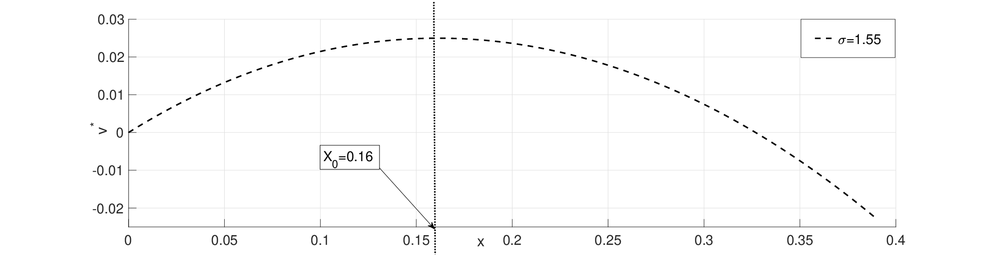
Our approach is inspired by the seminal paper of Sannikov [24], in a more general setting. Our main contribution is to establish a one-to-one correspondence between the continuation value of the consortium and the contract (rent plus terminal) payments, using Backward Stochastic differential equations (BSDE) with terminal time, stochastic control and optimal stopping technics. As it is standard in the literature, we use the weak approach, that is the agent changes the distribution of the social value of the project, by making the probability measure depend on agent’s effort. We derive the Hamilton Jacobi Bellman variational inequality characterizing the public value function. Finally we provide numerical solutions using Howard algorithm. Our contribution is twofold: first we provide rigorous results, combining optimal stochastic control and optimal stopping in this context of moral hazard, which is a challenging task especially in this literature. Then we detail the procedure to compute the numerical solutions and we provide a numerical analysis of the characteristics of the optimal contracts (effort, rent, value function) as well as the sensitivity with respect to the diffusion coefficient $\sigma$ of the social value of the project.
The outline of the paper is as follows. In Section 2, we formulate the problem, using the weak approach and we describe the public and the consortium problems. In Section 3, we determine the incentive compatible contract and we provide the dynamics of the consortium objective function, using the BSDE technique. In Section 4, we derive the Hamilton Jacobi Bellman Variational Inequality associated to the public value function and we provide a verification theorem. Section 5 is devoted mainly to the numerical study of the Hamilton Jacobi Bellman Variational Inequality based on the Howard algorithm, and the computations of the optimal controls and the value functions. Technical results on BSDE with random horizon are postponed in the Appendix.

2 The Public Private Partnership model under moral hazard

In this section, we work under the weak formulation as it is done usually in the principal-agent literature. Let $W$ be a standard one dimensional Brownian motion defined on a probability space $(\Omega,\mathbb{P})$ , and $\mathbb{F}=(\mathcal{F}_{t})_{t\geq 0}$ is the filtration generated by $W$ , satisfying the usual conditions of right-continuity and completeness.
We introduce the social value of the project that is observed by the public

{X_{t}:=X_{0}+\sigma W_{t}},~t\geq 0,~\mathbb{P}~a.s

(2.1)

where

•

$X_{0}>0$ is the initial value of the project.
•

$\sigma>0$ is the volatility of the operational cost of the infrastructure maintenance, that is assumed to be constant.¹¹ 1 This could be generalized to a regular $\mathbb{F}$ -progressive map $\sigma(X_{t})$ , this will be further discussed in Section 4.2.

Remark 2.1

We could take $\sigma$ equal to $1$ in (2.1). If $\sigma\equiv 1$ , then $X$ is the canonical process defined on $\Omega$ the set of continuous paths starting from $X_{0}$ and $\mathbb{P}$ is the Wiener measure on $\Omega.$ In this paper, $\sigma\not\equiv 1$ and we study numerically the sensitivity of the value function, the optimal effort and the optimal rent to the volatility parameter $\sigma.$

In the weak formulation, the agent changes the distribution of the process $X$ , by making the underlying probability measure $\mathbb{P}^{A}$ depend on agent’s effort $A$ . We define the process $\gamma^{A}=(\gamma_{t}^{A})_{t\geq 0}$ by

\gamma_{t}^{A}:=\exp\left[\int_{0}^{t}\frac{\varphi(A_{s})}{\sigma}dW_{s}-\frac{1}{2}\int_{0}^{t}\left(\frac{\varphi(A_{s})}{\sigma}\right)^{2}ds\right]=\mathcal{E}\left[\int_{0}^{t}\frac{\varphi(A_{s})}{\sigma}dW_{s}\right]~t\geq 0,~\mathbb{P}~a.s

where $\varphi$ is specified hereafter. We denote by ${\cal{T}}$ the set of all $\mathbb{F}$ -stopping times and for $t\geq 0,~\mbox{we define the set }\mathcal{T}_{t}:=\{\tau\in\mathcal{T}\mbox{ such that }\tau\geq t\}$ . We fix $\hat{p}\in(2,\infty)$ and we consider

	$\displaystyle\mathcal{A}^{\hat{p}}$	$\displaystyle:=$	$\displaystyle\{(A_{s})_{s\geq 0}~\mathbb{F}\mbox{-progressively measurable process,}~A_{s}\geq 0~ds\otimes d\mathbb{P}~a.e.~$		(2.2)
			$\displaystyle\quad\mbox{such that}~\mathop{\rm ess\,sup}_{\tau\in\mathcal{T}_{t}}\mathbb{E}[(\frac{\gamma^{A}_{\tau}}{\gamma^{A}_{t}})^{\hat{p}}\|\mathcal{F}_{t}]<\infty,~\forall~t\geq 0\}.$		(2.2)

The probability measure $\mathbb{P}^{A}$ is defined by $\frac{d\mathbb{P}^{A}}{d\mathbb{P}}|_{\mathcal{F}_{t}}=\gamma^{A}_{t}$ for all $t\geq 0$ . Then, $\mathbb{P}^{A}$ and $\mathbb{P}$ are equivalent. By Girsanov’s theorem, the process $(W_{t}^{A})_{t\geq 0}$ defined by

W_{t}^{A}:=W_{t}-\int_{0}^{t}\dfrac{\varphi(A_{s})}{\sigma}ds,~\mbox{for}~t\geq 0

is a $\mathbb{P}^{A}$ -Brownian motion and the social value of the project is given by:

X_{t}=X_{0}+\int_{0}^{t}\varphi(A_{s})ds+\sigma W_{t}^{A},~t\geq 0,~\mathbb{P}~a.s.

(2.3)

The public observes the social value $X$ of the project, but she does not observe directly the effort of the consortium: this is a situation of moral hazard. She chooses the rent she will pay to the consortium to compensate him for his efforts and the operational costs that he supports. The public could end the contract at the date $\tau$ , where $\tau$ is a stopping time in ${\cal{T}}.$
A contract is a triplet $\Gamma=((R_{t})_{t},\tau,\xi)$ where $R$ , which represents the rent paid by the public, is a non-negative ${\mathbb{F}}$ -progressively measurable process, $\tau\in{\cal{T}}$ , and $\xi$ is a non negative ${\mathcal{F}}_{\tau}$ -mesurable random variable which represents the cost of stopping the contract.

Remark 2.2

Contrary to a strong formulation (cf. Hajjej et al. [13]), the filtrations $\mathbb{F}^{X}$ and $\mathbb{F}$ coincide in the weak formulation, where $\mathbb{F}^{X}$ is the filtration generated by the social value process $X$ and $\mathbb{F}$ is the Brownian filtration generated by the standard Brownian motion $W$ .

We now define the respective optimization problems for the consortium and the public. Let us first define the functions involved in the formulation of the optimization problems.

Assumption 2.3

$\bullet$

$\varphi$ is the function that models the marginal impact of the consortium’s efforts on the social value, $\varphi:[0,\infty)\rightarrow[0,\infty)$ is $C^{2}$ strictly concave, bounded, increasing, $\varphi(0)=0$ and $\varphi^{\prime}(0)>0$ . We denote by $\|\varphi\|_{\infty}:=\sup_{a\geq 0}\varphi(a)$ .
$\bullet$

The utility function of the consortium $U:[0,\infty)\rightarrow[0,\infty)$ is $C^{2}$ strictly concave increasing and satisfying $U(0)=0$ and Inada’s conditions $U^{\prime}(\infty)=0,~U^{\prime}(0)=\infty$ .
$\bullet$

$h$ is the cost of the effort for the consortium; $h:[0,\infty)\rightarrow[0,\infty)$ is $C^{2}$ , strictly convex increasing, $h(0)=0$ .

In this paper, the time preference parameter $\lambda$ of the consortium is not necessarily equal to $\delta$ the one of the public, in general it is usual to assume that the consortium is more impatient than the public ( $\lambda\geq\delta$ ).

Given a contract $\Gamma=((R_{t})_{t},\tau,\xi)$ offered by the principal, the consortium gives a best response in terms of an effort process $A$ : this is a Stackelberg leadership model. The consortium accepts the contract only if his expected payoff exceeds his reservation value $\underline{x}.$

Agent’s best response

A^{*}\in\argmax_{A\in\mathcal{A}^{C}_{\rho-{2\lambda}}}\mathbb{E}^{A}\left[\int_{0}^{\tau}e^{-{{\lambda}}s}(U(R_{s})-h(A_{s}))ds+e^{-{{\lambda}}\tau}U(\xi){{\mathbf{1}}_{\{\tau<\infty\}}}\right]

(2.4)

where $\mathbb{E}^{A}$ is the expectation under $\mathbb{P}^{A}$ , and for some $\rho>0,$

	$\displaystyle\mathcal{A}^{C}_{\rho-{2\lambda}}$	$\displaystyle:=$	$\displaystyle\Big\{(A_{s})_{s\geq 0}\in\mathcal{A}^{\hat{p}},~\mbox{such that}~\mathbb{E}^{\mathbb{P}}\left[{\int_{0}^{\infty}}e^{(\rho-{2\lambda})s}\|h(A_{s})\|^{2}ds\right]<\infty$
			$\displaystyle\quad\mbox{and}~\mathbb{E}^{\mathbb{P}}\left[{\int_{0}^{\infty}}e^{(\rho-{2\lambda})s}\|\varphi(A_{s})\|^{2}ds\right]<\infty\Big\},$

The objective function starting at time $t$ for the consortium is $\mathbb{P}^{A}$ -a.s.

J_{t}^{C}(\Gamma,A):=\mathbb{E}^{A}\left[\int_{t}^{\tau}e^{-{{{\lambda}}(s-t)}}(U(R_{s})-h(A_{s}))ds+e^{-{{\lambda}}(\tau-t)}{U(\xi)}{{\mathbf{1}}_{\{\tau<\infty\}}}|\mathcal{F}_{t}\right].

As the process $(J_{t}^{C}(\Gamma,A))_{0\leq t\leq\tau}$ , is continuous and $\mathbb{P}^{A}\sim\mathbb{P}$ , we have

J_{t}^{C}(\Gamma,A)=\mathbb{E}^{A}\left[\int_{t}^{\tau}e^{-{{{\lambda}}(s-t)}}(U(R_{s})-h(A_{s}))ds+e^{-{{\lambda}}(\tau-t)}{U(\xi)}{{\mathbf{1}}_{\{\tau<\infty\}}}|\mathcal{F}_{t}\right],~\forall t\in[\![0,\tau]\!],~\mathbb{P}~a.s.

(2.5)

in which $[\![.,.]\!]$ denotes a stochastic interval.

Given the best response of the agent, the public entity (the principal) aims to maximize the social value of the project minus the rent. Since $\mathbb{E}^{{A}}\left[\int_{0}^{\tau}e^{-\delta s}dX_{s}\right]=\mathbb{E}^{{A}}\left[\int_{0}^{\tau}e^{-\delta s}\varphi({A_{s}})ds\right]$ by Doob’s optional sampling theorem, the principal problem is formulated by

\displaystyle\sup_{\Gamma\in\mathcal{A}^{P}_{\rho-{2\lambda}}}\displaystyle\sup_{P^{A^{*}}\in{\mathcal{P}^{\Gamma}}}\mathbb{E}^{{A^{*}}}\left[\int_{0}^{\tau}e^{-\delta s}(\varphi({A_{s}^{*}})-R_{s})ds-e^{-\delta\tau}\xi{{\mathbf{1}}_{\{\tau<\infty\}}}\right]

(2.6)

subject to the reservation constraint

\mathbb{E}^{A^{*}}\left[\int_{0}^{\tau}e^{-{{{\lambda}}s}}(U(R_{s})-h({A_{s}^{*}}))ds+e^{-{{{\lambda}}}\tau}{U(\xi)}{{\mathbf{1}}_{\{\tau<\infty\}}}\right]\geq{\underline{x}}

with

$\displaystyle\mathcal{A}^{P}_{{\rho-{2\lambda}}}$	$\displaystyle:=$	$\displaystyle\Big\{((R_{s})_{s\geq 0},\tau,\xi)~\mbox{ : }~R~\mbox{ is }\mathbb{F}\mbox{-progressively measurable process,}$	(2.7)
		$\displaystyle~\quad R_{s}\geq 0~ds\otimes d\mathbb{P}~a.e.\mbox{ and }~\mathbb{E}^{\mathbb{P}}\left[{\int_{0}^{\infty}}e^{(\rho-{2\lambda})s}(U(R_{s})^{2}\vee R_{s}^{2})ds\right]<\infty,$
		$\displaystyle\quad\tau\in\mathcal{T},~\xi\geq 0~\mathcal{F}_{\tau}\mbox{-measurable s.t. }~\mathbb{E}^{\mathbb{P}}\left[e^{(\rho-{2\lambda})\tau}({U(\xi)^{2}\vee}\xi^{2}){\mathbf{1}}_{\{\tau<\infty\}}\right]<\infty\Big\},$

where $x\vee y:=\max(x,y)$ and

\displaystyle{\mathcal{P}^{\Gamma}}:=\left\{\mathbb{P}^{A^{*}}\sim\mathbb{P},A^{*}\in\argmax_{A\in\mathcal{A}^{C}_{{\rho-{2\lambda}}}}\mathbb{E}^{A}\left[\int_{0}^{\tau}e^{-{{\lambda}}s}(U(R_{s})-h(A_{s}))ds+e^{-{{\lambda}}\tau}{U(\xi)}{{\mathbf{1}}_{\{\tau<\infty\}}}\right]\right\}.

The objective function starting at time $t$ for the public is $\mathbb{P}^{A^{*}}$ -a.s.

J_{t}^{P}(\Gamma,{A^{*}}):=\mathbb{E}^{A^{*}}\left[\int_{t}^{\tau}e^{-\delta(s-t)}(\varphi({A_{s}^{*}})-R_{s})ds-e^{-\delta(\tau-t)}\xi{{\mathbf{1}}_{\{\tau<\infty\}}}|\mathcal{F}_{t}\right].

Using the same arguments as in (2.5), we have

J_{t}^{P}(\Gamma,{A^{*}})=\mathbb{E}^{A^{*}}\left[\int_{t}^{\tau}e^{-\delta(s-t)}(\varphi({A_{s}^{*}})-R_{s})ds-e^{-\delta(\tau-t)}\xi{{\mathbf{1}}_{\{\tau<\infty\}}}|\mathcal{F}_{t}\right],~\forall t\in[\![0,\tau]\!],~\mathbb{P}~a.s.

(2.8)

3 Incentive compatible contracts

The aim of this section is to determine the incentive compatible contracts and to provide the dynamics of the consortium objective function $J^{C}$ . To achieve this, one first needs to prove an existence and uniqueness result for a certain type of BSDE with random horizon.
As we will see later, the objective function for the agent is related to the solution of the following BSDEs with a random time horizon $\tau$

Y_{t}={\zeta}{{\mathbf{1}}_{\{\tau<\infty\}}}+\int_{t}^{\tau}g(s,\omega,Z_{s})ds-\int_{t}^{\tau}Z_{s}dW_{s},

(3.1)

where the generator $g:\mathbb{R}_{+}\times\Omega\times\mathbb{R}\rightarrow\mathbb{R}$ does not depend on $Y$ .
BSDEs with random horizon have been studied by some authors. Chen [5] considered a random horizon which could be infinite and assumed that the constant of Lipschitz of the generator is time-dependent and square integrable on $[0,\infty]$ : this assumption is not satisfied in our case, since the Lipschitz coefficient $C_{g}$ is constant. Darling and Pardoux [10] studied a BSDE with finite random horizon. In our case, we cover the finite and the infinite random horizon. We give in the Appendix the proof of the existence and uniqueness of a solution to the BSDE (3.1), under the following assumptions

(H1(

\kappa

))

The generator $g:[0,\infty)\times\Omega\times\mathbb{R}\longrightarrow\mathbb{R}$ satisfies, for each $z\in\mathbb{R}$ , $g(.,.,z)$ is a progressively measurable process and for some $\kappa\in\mathbb{R}$ , we have

\mathbb{E}\left[e^{{\kappa}\tau}|\zeta|^{2}{{\mathbf{1}}_{\{\tau<\infty\}}}+\int_{0}^{\tau}e^{{\kappa}s}|g(s,\omega,0)|^{2}ds\right]<\infty.

(H2)

$g$ is Lipschitz with respect to $z$ , i.e. there exists a constant $C_{g}>0$ such that

$|g(s,\omega,z_{1})-g(s,\omega,z_{2})|\leq C_{g}|z_{1}-z_{2}|~ds\otimes d\mathbb{P}~{a.e.}$

We introduce the following spaces for a fixed stopping time $\tau\in\mathcal{T}$ and for some ${\kappa\in\mathbb{R}}$ :

$\displaystyle\mathcal{S}^{2}_{\kappa}(\tau):$	$\displaystyle=$	$\displaystyle\{{Y}~\mathbb{R}\mbox{-valued,}~\mathbb{F}\mbox{-progressively measurable continuous process such that}$
		$\displaystyle~~~~~~~~~~~~\|\|{Y}\|\|_{{\cal S}^{2}_{\kappa}(\tau)}:=\left(\mathbb{E}^{\mathbb{P}}\left[\displaystyle\sup_{0\leq s\leq\tau}e^{{\kappa}s}\|{Y}_{s}\|^{2}\right]\right)^{\frac{1}{2}}<\infty\},$
$\displaystyle{\cal H}^{2}_{\kappa}(\tau):$	$\displaystyle=$	$\displaystyle\{{Z}~\mathbb{R}\mbox{-valued,}~\mathbb{F}\mbox{-progressively measurable process such that}$
		$\displaystyle~~~~~~~~~~~~\|\|{Z}\|\|_{{\cal H}^{2}_{\kappa}(\tau)}:=\left(\mathbb{E}^{\mathbb{P}}\left[\int_{0}^{\tau}e^{{\kappa}s}\|{Z}_{s}\|^{2}ds\right]\right)^{\frac{1}{2}}<\infty\},$
$\displaystyle{L}^{2}_{\kappa}(\mathcal{F}_{\tau}):$	$\displaystyle=$	$\displaystyle\{\zeta~\mathbb{R}\mbox{-valued,}~\mathcal{F}_{\tau}\mbox{-measurable random variable such that}~\mathbb{E}\left[e^{{\kappa}\tau}\|{\zeta}\|^{2}{{\mathbf{1}}_{\{\tau<\infty\}}}\right]<\infty\}.$

The main result of Section 3 is the following theorem.

Theorem 3.1

Suppose Assumption 2.3 and $\rho>\frac{\|\varphi\|_{\infty}^{2}}{\sigma^{2}}$ , then
(i) There exists $Z\in{\cal H}^{2}_{\rho}(\tau)$ and a function $A^{*}:\mathbb{R}\longrightarrow\mathbb{R}$ such that the optimal effort satisfies

A^{*}_{t}=A^{*}(Z_{t}),~\forall t\in[\![0,\tau[\![,~\mathbb{P}~a.s.

(3.2)

(ii) For any admissible contract $\Gamma\in\mathcal{A}^{P}_{\rho-2\lambda}$ , the consortium value function $(J_{t}^{C}(\Gamma,A^{*}(Z)))_{t}$ solves the BSDE with random horizon:

	$\displaystyle dJ_{t}^{C}(\Gamma,A^{*}(Z))$	$\displaystyle=$	$\displaystyle-\Big(-{{\lambda}}J_{t}^{C}(\Gamma,A^{}(Z))+U(R_{t})+\psi(A^{}(Z_{t}),Z_{t})\Big)dt+Z_{t}dW_{t},$		(3.3)
	$\displaystyle J_{\tau}^{C}(\Gamma,A^{*}(Z))$	$\displaystyle=$	$\displaystyle{U(\xi)}{{\mathbf{1}}_{\{\tau<\infty\}}}$

where

\psi(a,z):=-h(a)+{z}\frac{\varphi(a)}{\sigma}.

(3.4)

The proof is split in several lemmas and propositions, with first the existence and unicity of BSDE (3.3). By a change of variable, this is related to the existence and uniqueness of a solution to the BSDE (3.1) which is given in the following proposition.

Proposition 3.2

Let $\tau$ be a stopping time in $\mathcal{T}$ and $\rho>C^{2}_{g}$ . If ${\zeta\in{L}^{2}_{\rho}(\mathcal{F}_{\tau})},~g$ satisfies Assumptions (H1( $\rho$ )) and (H2), there exists a unique solution $(Y,Z)\in\mathcal{S}^{2}_{\rho}(\tau)\times{\cal H}^{2}_{\rho}(\tau)$ to the BSDE (3.1).

The proof is postponed in the Appendix. In our setting, the constant $C^{2}_{g}$ will be $\frac{\|\varphi\|_{\infty}^{2}}{\sigma^{2}}$ .
Thanks to the boundedness of the function $\varphi$ , the generator of the BSDE that the consortium value function must satisfy is Lipschitz with respect to the variable $z$ . To the best of our knowledge, such condition is crucial to prove the existence of a unique pair $(Y,Z)$ satisfying a BSDE with random horizon (see Darling and Pardoux [10]).
Proposition 3.2 is used to determine the incentive compatible contract and to provide the dynamics of the consortium objective function. This is useful in what follows in order to reformulate the optimization problems in terms of the consortium objective function $J^{C}$ .

Lemma 3.3

Suppose Assumption 2.3 and $\rho>\frac{\|\varphi\|_{\infty}^{2}}{\sigma^{2}}$ . For any admissible contract $\Gamma\in\mathcal{A}^{P}_{\rho-2\lambda}$ and for any $A\in\mathcal{A}^{C}_{\rho-2\lambda}$ , there exists $Z^{A}\in{\mathcal{H}^{2}_{\rho-{2\lambda}}(\tau)}$ such that the dynamics of the consortium objective function evolves according to the BSDE with random terminal condition

dJ_{t}^{C}(\Gamma,A)=-\Big(-{{\lambda}}J_{t}^{C}(\Gamma,A)+U(R_{t})+\psi(A_{t},Z_{t}^{A})\Big)dt+Z_{t}^{A}dW_{t},~J_{\tau}^{C}(\Gamma,A)={U(\xi)}{{\mathbf{1}}_{\{\tau<\infty\}}}

(3.5)

where $\psi$ is defined in (3.4).

Proof: For any admissible contract $\Gamma\in\mathcal{A}^{P}_{\rho-2\lambda},$ for any $A\in\mathcal{A}^{C}_{\rho-2\lambda}$ and for any $t\in[\![0,\tau[\![$ , we define the integrable process

\begin{array}[]{rcl}M_{t}^{C}(\Gamma,A):&=&~e^{-\lambda t}J_{t}^{C}(\Gamma,A)+\int_{0}^{t}e^{-\lambda s}(U(R_{s})-h(A_{s}))ds\\ &=&\mathbb{E}^{\mathbb{P}^{A}}\left[\int_{0}^{\tau}e^{-\lambda s}(U(R_{s})-h(A_{s}))ds+e^{-\lambda\tau}U(\xi){{\mathbf{1}}_{\{\tau<\infty\}}}|\mathcal{F}_{t}\right]\\ &=&\dfrac{1}{\gamma_{t}^{A}}\mathbb{E}^{\mathbb{P}}\left[\gamma_{\tau}^{A}\int_{0}^{\tau}e^{-\lambda s}(U(R_{s})-h(A_{s}))ds+\gamma_{\tau}^{A}e^{-\lambda\tau}U(\xi){{\mathbf{1}}_{\{\tau<\infty\}}}|\mathcal{F}_{t}\right],\end{array}

where the last equality is obtained using Bayes formula.
As $\big(\mathbb{E}^{\mathbb{P}}\left[\gamma_{\tau}^{A}(\int_{0}^{\tau}e^{-\lambda s}(U(R_{s})-h(A_{s}))ds+e^{-\lambda\tau}U(\xi){{\mathbf{1}}_{\{\tau<\infty\}}})|\mathcal{F}_{t}\right]\big)$ is a ( $\mathbb{P}$ , $\mathbb{F})$ -local martingale, by the martingale representation theorem, there exists an $\mathbb{F}$ -progressively measurable process $\chi$ such that: ²² 2 It is important to work under the probability measure $\mathbb{P}$ and not $\mathbb{P}^{A}$ . Indeed, although the inclusion $\mathbb{F}^{A}=\sigma(W^{A})\subseteq\mathbb{F}$ holds, the reverse inclusion is not true in general case (see the Tsirel’son’s example in [26]).

M_{t}^{C}(\Gamma,A)=\dfrac{1}{\gamma^{A}_{t}}\left(M_{0}^{C}(\Gamma,A)+\int_{0}^{t}\chi_{s}dW_{s}\right).

Thus $d(\gamma_{t}^{A}M_{t}^{C}(\Gamma,A))=\chi_{t}dW_{t},$ using Itô’s formula, we obtain

M_{t}^{C}(\Gamma,A)=M_{0}^{C}(\Gamma,A)+\int_{0}^{t}\left(\frac{\chi_{s}}{\gamma_{s}^{A}}{-}M_{s}^{C}(\Gamma,A)\frac{\varphi(A_{s})}{\sigma}\right)dW_{s}^{A}.

Then denoting $Z_{s}^{A}=e^{{\lambda}s}(\frac{\chi_{s}}{\gamma_{s}^{A}}{-}M_{s}^{C}(\Gamma,A)\frac{\varphi(A_{s})}{\sigma})~ds\otimes d\mathbb{P}$ a.e, we deduce

e^{-\lambda t}J_{t}^{C}(\Gamma,A)=M_{0}^{C}(\Gamma,A)-\int_{0}^{t}e^{-{\lambda}s}(U(R_{s})-h(A_{s}))ds+\int_{0}^{t}e^{-{\lambda}s}Z_{s}^{A}dW_{s}^{A},

and we obtain

dJ_{t}^{C}(\Gamma,A)=-\Big(-{\lambda}J_{t}^{C}(\Gamma,A)+U(R_{t})-h(A_{t})\Big)dt+Z_{t}^{A}dW_{t}^{A},

which implies that under $\mathbb{P}$

dJ_{t}^{C}(\Gamma,A)=-\left({-{\lambda}}J_{t}^{C}(\Gamma,A)+U(R_{t})-h(A_{t})+Z_{t}^{A}\frac{\varphi(A_{t})}{\sigma}\right)dt+Z_{t}^{A}dW_{t},~J_{\tau}^{C}(\Gamma,A)={U(\xi)}{{\mathbf{1}}_{\{\tau<\infty\}}}.

(3.6)

The associated Backward Stochastic Differential Equation (BSDE $(A,R,\tau,\xi)$ in short) is given by

\displaystyle\left\{\begin{array}[]{ll}dY_{t}&=-\left(-{\lambda}Y_{t}+U(R_{t})+\psi(A_{t},Z_{t}^{A})\right)dt+Z_{t}^{A}dW_{t},\\ Y_{\tau}&={U(\xi)}{{\mathbf{1}}_{\{\tau<\infty\}}},\end{array}\right.

where $\psi$ is defined by (3.4). Considering the discounted quantities

(\tilde{Y}_{t},\tilde{Z}_{t}^{A})=(e^{-\lambda t}Y_{t},e^{-\lambda t}Z_{t}^{A}),~t\in[\![0,\tau[\![,~\mathbb{P}~a.s,

$(\tilde{Y},\tilde{Z}^{A})$ satisfies the BSDE

\displaystyle\left\{\begin{array}[]{ll}d\tilde{Y}_{t}&=-\left(\tilde{U}(R_{t})+\tilde{\psi}(A_{t},\tilde{Z}_{t}^{A})\right)dt+\tilde{Z}^{A}_{t}dW_{t},\\ \tilde{Y}_{\tau}&={\tilde{U}(\xi)}{{\mathbf{1}}_{\{\tau<\infty\}}},\end{array}\right.

where

\displaystyle\left\{\begin{array}[]{ll}{\tilde{h}(A_{t})}&:=e^{-\lambda t}h(A_{t}),\\ \tilde{U}(R_{t})&:=e^{-\lambda t}U(R_{t}),\\ \tilde{U}(\xi)&:=e^{-\lambda t}U(\xi)\\ \tilde{\psi}(A_{t},{\tilde{Z}}_{t}^{A})&:=-{\tilde{h}(A_{t})}+\tilde{Z}_{t}^{A}\frac{\varphi(A_{t})}{\sigma}.\\ \end{array}\right.

The generator of the BSDE (3) depends only on $\tilde{Z}^{A}$ and is defined by $g(t,\omega,z):=\tilde{U}(R_{t})-{\tilde{h}(A_{t})}+z\frac{\varphi(A_{t})}{\sigma}.$ From the definition of the sets $\mathcal{A}^{C}_{\rho-2\lambda}$ and $\mathcal{A}^{P}_{\rho-2\lambda}$ , the generator $g:\mathbb{R}_{+}\times\Omega\times\mathbb{R}\rightarrow\mathbb{R}$ satisfies $(H1(\rho))$ and $g$ satisfies $(H2)$ since $\varphi$ is bounded. Then from Proposition 3.2, there exists a unique $(\tilde{Y},\tilde{Z}^{A})\in\mathcal{S}^{2}_{\rho}(\tau)\times\mathcal{H}^{2}_{\rho}(\tau)$ solving the BSDE (3). Therefore, there exists a unique $(Y,Z^{A})$ solving the BSDE (3) such that

\left(\mathbb{E}^{\mathbb{P}}\left[\displaystyle\sup_{0\leq s\leq\tau}e^{(\rho-2\lambda)s}|Y_{s}|^{2}\right]\right)^{\frac{1}{2}}<\infty~\mbox{and}~\left(\mathbb{E}^{\mathbb{P}}\left[\int_{0}^{\tau}e^{(\rho-2\lambda)s}|Z_{s}^{A}|^{2}ds\right]\right)^{\frac{1}{2}}<\infty,

i.e. ${(Y,Z^{A})\in\mathcal{S}^{2}_{\rho-2\lambda}(\tau)\times\mathcal{H}^{2}_{\rho-2\lambda}(\tau)}$ . $\bullet$
We are interested in BSDE (3) for which we prove a classic comparison theorem, that is postponed in the Appendix (see Theorem 6.1). We deduce the following Corollary 3.4, which is a direct consequence of the comparison theorem.

Corollary 3.4

For any $A\in\mathcal{A}^{C}_{\rho-2\lambda}$ and for any admissible contract $\Gamma\in\mathcal{A}^{P}_{\rho-2\lambda}$ , if there exists $A^{*}\in\mathcal{A}^{C}_{\rho-2\lambda}$ such that $\psi(A_{t},Z_{t}^{A})\leq\psi(A^{*}_{t},Z_{t}^{A})~\forall t\in[\![0,\tau[\![~\mathbb{P}~a.s.,$ then

J_{t}^{C}(\Gamma,A)\leq J_{t}^{C}(\Gamma,A^{*}),~\mbox{for all}~t\in[\![0,\tau[\![,~\mathbb{P}~a.s.,

where $(J_{t}^{C}(\Gamma,A^{*}))_{t\geq 0}$ satisfies

\left\{\begin{array}[]{ll}dJ_{t}^{C}(\Gamma,A^{*})&=-\Big(-{{\lambda}}J_{t}^{C}(\Gamma,A^{*})+U(R_{t})+\psi(A^{*}_{t},Z_{t}^{A})\Big)dt+Z_{t}^{A}dW_{t},\\ J_{\tau}^{C}(\Gamma,A^{*})&={U(\xi)}{{\mathbf{1}}_{\{\tau<\infty\}}}.\end{array}\right.

(3.18)

The following lemma is technical and will be useful later to parametrize the optimal response $A^{*}$ as a deterministic function of $Z^{A}$ for $A$ admissible control.

Lemma 3.5

Suppose Assumption 2.3. Let define $A^{*}(z):=\arg\displaystyle\max_{a\geq 0}\psi(a,z)$ , for $z\in\mathbb{R}$ .
If $z>\sigma\frac{h^{\prime}(0)}{\varphi^{\prime}(0)},$ then $A^{*}(z)=(\frac{h^{\prime}}{\varphi^{\prime}})^{-1}(\frac{z}{\sigma})$ and if $z\leq\sigma\frac{h^{\prime}(0)}{\varphi^{\prime}(0)},$ then $A^{*}(z)=0.$
Moreover, $A^{*}$ is a bijection from $\{0\}\cup(\sigma\frac{h^{\prime}}{\varphi^{\prime}}(0),\infty)$ to $[0,\infty).$

Proof: We fix $z\in\mathbb{R}$ . Under Assumption 2.3, $~(\frac{h^{\prime}}{\varphi^{\prime}})^{{}^{\prime}}(a)=\dfrac{h^{\prime\prime}(a)\varphi^{\prime}(a)-\varphi^{\prime\prime}(a)h^{\prime}(a)}{(\varphi^{\prime}(a))^{2}}>0$ for all $a\geq 0$ . This shows that $\frac{h^{\prime}}{\varphi^{\prime}}$ is invertible from $[0,\infty)$ into $[\frac{h^{\prime}(0)}{\varphi^{\prime}(0)},\infty).$
First case: $z>\sigma\frac{h^{\prime}(0)}{\varphi^{\prime}(0)}$ . The function $\psi$ , defined in Equation (3.4), is strictly concave, the first-order necessary condition of optimality $\frac{\partial\psi}{\partial a}({A^{*}(z)},z)=0$ is sufficient and is equivalent to

z=\sigma\frac{h^{\prime}(A^{*}(z))}{\varphi^{\prime}(A^{*}(z))}.

(3.19)

Thus $A^{*}$ is a bijection from $(\sigma\frac{h^{\prime}}{\varphi^{\prime}}(0),\infty)$ to $(0,\infty).$
Second case: $0<z\leq\sigma\frac{h^{\prime}(0)}{\varphi^{\prime}(0)}$ . Then Equation (3.19) is not well defined. The optimum could not be positive. In the neighborhood of $0$ , the function $\psi$ must be decreasing, otherwise $A^{*}(z)=0$ is not a maximum. The necessary condition of optimality $\frac{\partial\psi}{\partial a}(0,z)=-h^{\prime}(0)+z\frac{\varphi^{\prime}(0)}{\sigma}\leq 0$ is satisfied in $0$ . As the function $\psi$ is strictly concave, the latter condition is sufficient. This shows that $A^{*}(z)=0.$
Third case: $z\leq 0$ . The function $\psi(z,.)$ is decreasing in $a$ and so $A^{*}(z)=0.$ In particular, $A^{*}(0)=0,$ and so Lemma 3.5 is proved. $\bullet$

The following proposition gives a representation of the optimal effort. This step is crucial to transform the initial non-standard stochastic control problem into a standard one.

Proposition 3.6

Let $\Gamma\in\mathcal{A}^{P}_{\rho-2\lambda}$ and $A\in\mathcal{A}^{C}_{\rho-2\lambda}.$ There exists a bijection between the process $(Z_{t}^{A})_{t\geq 0}$ and the optimal effort $(A^{*}_{t})_{t\geq 0},$ the bijection is given by

A^{*}_{t}=A^{*}(Z_{t}^{A})=(\frac{h^{\prime}}{\varphi^{\prime}})^{-1}(\frac{Z_{t}^{A}}{\sigma}){\mathbf{1}}_{\{Z^{A}_{t}>0\}},

or equivalently

Z_{t}^{A}=(\sigma\frac{h^{\prime}}{\varphi^{\prime}})(A^{*}(Z_{t}^{A})){\mathbf{1}}_{\{A^{*}(Z_{t}^{A})>0\}}.

Proof: We consider the stochastic set $\mathcal{D}=\{(t,\omega),{A^{*}_{t}}(\omega)>0\}.$ From Lemma 3.5, we have $Z_{t}^{A}=\sigma\frac{h^{\prime}(A^{*}_{t})}{\varphi^{\prime}(A^{*}_{t})}$ . As $h$ and $\varphi$ are increasing (see Assumption 2.3), $(Z_{t}^{A})_{t\geq 0}$ is a positive process. The function $\frac{h^{\prime}}{\varphi^{\prime}}$ being invertible gives a bijection between $Z_{t}^{A}$ and $A_{t}^{*}$ .
Now we consider $\mathcal{D}^{C}:=\{(t,\omega),A^{*}_{t}(\omega)=0\}.$ On this set, from Lemma 3.5, we have $Z_{t}^{A}\leq\sigma\frac{h^{\prime}(0)}{\varphi^{\prime}(0)}$ .
From the definition of the objective function for the public, and since the rent is non-negative, $R_{t}^{*}=0$ on $\mathcal{D}^{C}.$ For $(t,\omega)\in\mathcal{D}^{C}$ , the consortium does not receive any rent from the public and does not provide any effort, we have from Equation (3.18)

\displaystyle dJ_{t}^{C}(R^{*},\tau,\xi,A^{*})

\displaystyle=

\displaystyle-\Big(-\lambda J_{t}^{C}(R^{*},\tau,\xi,A^{*})+\frac{Z^{A}_{t}}{\sigma}\varphi(A^{*}_{t})\Big)dt+Z_{t}^{A}dW_{t}.

On the other hand, for $(t,\omega)\in\mathcal{D}^{C}$ , $e^{-\lambda t}J_{t}^{C}(R^{*},\tau,\xi,A^{*})$ is constant since $R_{t}^{*}=A_{t}^{*}=0$ , which yields

\displaystyle dJ_{t}^{C}(R^{*},\tau,\xi,A^{*})

\displaystyle=

\displaystyle\lambda J_{t}^{C}(R^{*},\tau,\xi,A^{*})dt.

The uniqueness of the Itô decomposition implies $Z^{A}_{t}=0~a.s.$ This shows $A_{t}^{*}=A^{*}(Z_{t}^{A})=(\frac{h^{\prime}}{\varphi^{\prime}})^{-1}(\frac{Z^{A}_{t}}{\sigma}){\mathbf{1}}_{\{Z_{t}^{A}>0\}}$ . $\bullet$

Proposition 3.7

Suppose Assumption 2.3. We assume that the generator defined by $(t,\omega,z)\mapsto g(t,\omega,z):=\tilde{U}(R_{t})-{\tilde{h}(A^{*}(e^{\lambda t}z))}+z\frac{\varphi(A^{*}(e^{\lambda t}z))}{\sigma}$ satisfies the Assumptions $(H1(\rho))$ and $(H2$ ) with Lipschitz coefficient $C_{g}$ satisfying $C_{g}^{2}<\rho$ . Then, the dynamics of $J^{C}$ for any incentive compatible contract $(\Gamma,A^{*}(Z))$ (with $\Gamma\in{\cal A}^{P}_{\rho-2\lambda}$ and $A^{*}(Z)\in{\cal A}^{C}_{\rho-2\lambda})$ is given by the BSDE with random terminal condition

	$\displaystyle dJ_{t}^{C}(\Gamma,A^{*}(Z))$	$\displaystyle=$	$\displaystyle-\Big(-{{\lambda}}J_{t}^{C}(\Gamma,A^{}(Z_{t}))+U(R_{t})+\psi(A^{}(Z_{t}),Z_{t})\Big)dt+Z_{t}dW_{t},$
	$\displaystyle~J_{\tau}^{C}(\Gamma,A^{*}(Z))$	$\displaystyle=$	$\displaystyle{U(\xi)}{{\mathbf{1}}_{\{\tau<\infty\}}},$		(3.20)

where $A^{*}(Z)$ is defined in Lemma 3.5.

Proof: For $\Gamma\in{\cal A}^{P}_{\rho-2\lambda}$ and $A^{*}(Z)\in{\cal A}^{C}_{\rho-2\lambda}$ , we consider the BSDE

dY_{t}=-\Big(-{{\lambda}}Y_{t}+U(R_{t})+\psi(A^{*}(Z_{t}),Z_{t})\Big)dt+Z_{t}dW_{t},~Y_{\tau}={U(\xi)}{{\mathbf{1}}_{\{\tau<\infty\}}}.

(3.21)

Or equivalently

\displaystyle d\tilde{Y}_{t}=-\left(\tilde{U}(R_{t})-\tilde{h}(A^{*}(e^{\lambda t}\tilde{Z}_{t}))+\tilde{Z}_{t}\frac{\varphi(A^{*}(e^{\lambda t}\tilde{Z}_{t}))}{\sigma}\right)dt+\tilde{Z}_{t}dW_{t},\,~\tilde{Y}_{\tau}=e^{-\lambda\tau}{U(\xi)}{{\mathbf{1}}_{\{\tau<\infty\}}}.

(3.22)

From the statement of the Proposition, Assumptions $(H1(\rho))$ and $(H2)$ are satisfied. From Proposition 3.2, there exists a unique solution $(\tilde{Y},\tilde{Z})\in\mathcal{S}^{2}_{\rho}(\tau)\times{\cal H}^{2}_{\rho}(\tau)$ to the BSDE (3.22) or equivalently there exists a unique $(Y,Z)\in{\mathcal{S}^{2}_{\rho-2\lambda}(\tau)\times\mathcal{H}^{2}_{\rho-2\lambda}(\tau)}$ which solves (3.21). On the other hand, as $\left(\mathbb{E}^{\mathbb{P}}\left[\gamma_{\tau}^{A^{*}(Z)}\left(\int_{0}^{\tau}e^{-\lambda s}(U(R_{s})-h(A^{*}(Z_{s})))ds+e^{-\lambda\tau}{U(\xi)}{{\mathbf{1}}_{\{\tau<\infty\}}}\right)|\mathcal{F}_{t}\right]\right)$ is a ( $\mathbb{P}$ , $\mathbb{F})$ - local martingale, by applying the martingale representation theorem as in Lemma 3.3, there exists a progressively measurable process $(Z_{t}^{A^{*}(Z)})_{t}$ such that:

$\displaystyle dJ_{t}^{C}(\Gamma,A^{*}(Z))$	$\displaystyle=$	$\displaystyle-\left(-{{\lambda}}J_{t}^{C}(\Gamma,A^{}(Z))+U(R_{t})-h(A^{}(Z_{t}))+Z_{t}^{A^{}(Z)}\frac{\varphi(A^{}(Z_{t}))}{\sigma}\right)dt$
	$\displaystyle+$	$\displaystyle Z_{t}^{A^{*}(Z)}dW_{t},$
$\displaystyle J_{\tau}^{C}(\Gamma,A^{*}(Z^{A}))$	$\displaystyle=$	$\displaystyle{U(\xi)}{{\mathbf{1}}_{\{\tau<\infty\}}}.$

The uniqueness of the solution yields that

Z_{t}=Z_{t}^{A^{*}(Z)},~\mathbb{P}~a.s,~{\forall t\in[\![0,\tau[\![}.

Moreover, as $\tilde{\psi}(A^{*}(e^{\lambda t}\tilde{Z}_{t}),\tilde{Z}_{t})\geq\tilde{\psi}(A_{t},\tilde{Z}_{t})~\mathbb{P}~a.s~\forall t\in[\![0,\tau[\![~{\forall A\in\mathcal{A}^{C}_{\rho-2\lambda}~}$ , by Corollary 3.4 we have for all $A\in\mathcal{A}^{C}_{\rho-2\lambda}$

J_{t}^{C}(\Gamma,A)\leq J_{t}^{C}(\Gamma,A^{*}(Z)),~\forall t\in[\![0,\tau[\![~{}\mathbb{P}~a.s.

$\bullet$

Remark 3.8

According to Proposition 3.7, for any contract $\Gamma\in{\cal A}^{P}_{\rho-2\lambda}$ and in particular any terminal payment $\xi\in L^{2}_{\rho-2\lambda}(\mathcal{F}_{\tau})$ at time $\tau$ , $U(\xi)$ can be represented as the terminal value of a stochastic process $(\zeta_{t})_{t\geq 0}$ characterized by its initial value $\zeta_{0}$ and its diffusion coefficient $Z_{t}$ , its drift being given by $\left(-{{\lambda}}\zeta_{t}+U(R_{t})+\psi(A^{*}(Z_{t}),Z_{t})\right)$ . Observe that the optimal effort $A^{*}(Z)$ is then function of the diffusion process $Z$ , which is $\mathbb{F}$ -adapted, that is measurable with respect to the filtration generated by the social welfare $X$ of the project. This means that $Z$ has to be chosen by the public in an optimal way (and indexed on the social welfare $X$ ) in order to incentive the consortium to provide the greatest effort. Of course this contract should be chosen in the set of acceptable contracts to the consortium, that is the initial value $\zeta_{0}$ should be greater than the reservation constraint $\underline{x}$

J_{0}^{C}(\Gamma,A^{*}(Z))=\zeta_{0}=\mathbb{E}^{A^{*}(Z)}\left[\int_{0}^{\tau}e^{-{{{\lambda}}s}}(U(R_{s})-h(A^{*}(Z_{s})))ds+e^{-{{\lambda}}\tau}U(\xi){{\mathbf{1}}_{\{\tau<\infty\}}}\right]\geq\underline{x}.

Remark also that the incentive comes from both the rent and the terminal payment. Thus we could not obtain an explicit form for the terminal payment as a function of the terminal social welfare, as it can be done for a unique lumpsum and in some particular cases (see [15]). Here the optimal contract is given in a feedback form using a verification theorem, as in Sannikov [24].

Corollary 3.9

For $\Gamma\in\mathcal{A}^{P}_{\rho-2\lambda}$ and $A^{*}(Z)\in\mathcal{A}^{C}_{\rho-2\lambda}$ the best response, the objective function $J_{t}^{C}(\Gamma,A^{*}(Z))$ satisfies

J_{t}^{C}(\Gamma,A^{*}(Z))\geq 0~\forall t\in[\![0,\tau[\![,~\mathbb{P}~a.s.

Proof: We consider the contract $\Gamma=(R,\tau,\xi)\in\mathcal{A}^{P}_{\rho-2\lambda}$ and $A^{*}(Z)\in\mathcal{A}^{C}_{\rho-2\lambda}$ the best response, then as the consortium can guarantee himself non-negative utility by taking an effort equal to zero, the consortium objective function is non-negative, i.e., we have

J_{t}^{C}(\Gamma,A^{*}(Z))\geq 0,~\forall t\in[\![0,\tau[\![,~\mathbb{P}~a.s.

$\bullet$

Remark 3.10

Here are the functions used in our numerical study. As stated before, it is natural to consider an increasing concave function $\varphi$ for the impact of the effort on the social value, and an increasing convex function $h$ for the cost of the effort. We take them positive and of exponential form, namely $\varphi(x)=3(1-e^{-\alpha x})$ and $h(x)=e^{\beta x}-1$ , for positive real numbers $\alpha$ and $\beta$ . The coefficients $\alpha$ and $\beta$ are chosen such that the two functions have the same magnitude, in order to ensure a reasonable tradeoff between gain and cost. This implies the following generator of the BSDE (3.22)

\displaystyle g(t,\omega,z)=\left\{\begin{array}[]{ll}\tilde{U}(R_{t})+e^{-\lambda t}+\frac{z}{\sigma}-z^{\frac{\beta}{\alpha+\beta}}\bigg(\frac{1}{\sigma}\big(\frac{e^{\lambda t}\alpha}{\beta\sigma}\big)^{\frac{-\alpha}{\alpha+\beta}}+e^{-\lambda t}\big(\frac{e^{\lambda t}\alpha}{\beta\sigma}\big)^{\frac{\beta}{\alpha+\beta}}\bigg),~\mbox{if}~e^{\lambda t}z>\sigma\frac{\beta}{\alpha},\\ \tilde{U}(R_{t}),~\mbox{if}~e^{\lambda t}z\leq\sigma\frac{\beta}{\alpha}.\end{array}\right.

We check that the generator $g$ satisfies the Assumptions $(H1(\rho))$ and $(H2)$ for $\rho>C^{2}_{g}$ since
$\mathbb{E}\big[\int_{0}^{\tau}e^{\rho s}|g(s,\omega,0)|^{2}ds\big]=\mathbb{E}\big[\int_{0}^{\tau}e^{\rho s}|\tilde{U}(R_{s})|^{2}ds\big]=\mathbb{E}\big[\int_{0}^{\tau}e^{(\rho-2\lambda)s}|U(R_{s})|^{2}ds\big]<\infty$ as soon as the contract is in $\mathcal{A}^{P}_{\rho-2\lambda}$ . For the numerical study, we will choose such functions.

We now reformulate the stochastic control problem with $J^{C}$ as state variable and the contract $\Gamma$ and the best effort $A^{*}(Z)$ as control processes. Usually in the literature (see Sannikov [24] and Cvitanic et al. [7]), the optimization problem consists in maximizing a certain criterion where the control variables are given by $\Gamma$ and $(Z_{t})_{t\geq 0}$ which is a standard mixed stopping-regular stochastic control problem. In this paper, we keep the explicit control $(A^{*}(Z_{t}))_{t\geq 0}$ instead of $(Z_{t})_{t\geq 0}$ , since $(A^{*}(Z_{t}))_{t\geq 0}$ represents a physical quantity and thus it is more quantifiable and interpretable than the control $(Z_{t})_{t\geq 0}$ which is a diffusion coefficient.

4 Hamilton Jacobi Bellman variational inequality

From now on, we adopt a forward point of view for the dynamics of the consortium objective function which evolves according to the following forward SDE

	$\displaystyle dJ_{t}^{C}(x,R,\tau,A^{*}(Z))$	$\displaystyle=$	$\displaystyle\left({{\lambda}}J_{t}^{C}(x,R,\tau,A^{}(Z))-U(R_{t})+h(A^{}(Z_{t}))-Z_{t}\frac{\varphi(A^{*}(Z_{t}))}{\sigma}\right)dt+Z_{t}dW_{t},$
	$\displaystyle J_{0}^{C}(x,R,\tau,A^{*}(Z))$	$\displaystyle=$	$\displaystyle x\geq\underline{x}.$		(4.1)

Remark 4.1

As we choose an initial condition satisfying $J_{0}^{C}(x,R,\tau,A^{*}(Z))=x\geq\underline{x}$ , the reservation constraint formulated in the maximization problem of the public is satisfied. However, we solve the stochastic control problem related to the public on the whole domain i.e on $\mathbb{R}^{+}$ . In fact the consortium objective function at time $t$ , denoted by $J_{t}^{C}(x,R,\tau,A^{*}(Z))$ could be less than $\underline{x}$ although $J_{0}^{C}(x,R,\tau,A^{*}(Z))\geq\underline{x}$ .

Using the characterization of the incentive compatible contracts, the optimization problem of the public can be written as a standard stochastic control problem. The state process is the consortium objective function $J^{C}$ whose dynamics is given by (4). The control processes are given by $R$ , $\tau$ and $A^{*}(Z)\in\mathcal{A}^{C}_{\rho-2\lambda}$ and the value function given by (2.6) is formulated as:

v(x):=\sup_{(R,\tau,{{A^{*}(Z)}})\in{\cal{Y}}}\mathbb{E}^{{A^{*}(Z)}}_{x}\left[\int_{0}^{\tau}e^{-\delta s}(\varphi(A^{*}(Z_{s}))-R_{s})ds-e^{-\delta\tau}{U^{-1}}({J_{\tau}^{C}(x,R,\tau,A^{*}(Z))})\right],

(4.2)

where $\mathbb{E}^{A^{*}(Z)}_{x}$ is the conditional expectation with respect to the initial event $\{J_{0}^{C}(x,R,\tau,A^{*}(Z))=x\}$ and

	$\displaystyle{\cal{Y}}$	$\displaystyle:=$	$\displaystyle\Big\{(R,\tau,A^{*}(Z)):~R\geq 0~\mathbb{F}\mbox{-progressively measurable process s.t.}$		(4.3)
			$\displaystyle\,\,\,\mathbb{E}^{\mathbb{P}}[{\int_{0}^{\infty}}e^{{(\rho-2\lambda)}s}(U(R_{s})^{2}\vee R^{2}_{s})ds]<\infty,~\tau\in{\cal{T}},{A^{*}(Z)}\in\mathcal{A}^{C}_{\rho-2\lambda}\Big\}.$		(4.3)

The value function $v$ in (4.2) is defined on $\mathbb{R}^{+}$ since $J_{t}^{C}(\Gamma,A^{*}(Z))\geq 0$ by Corollary 3.9.
The set

{\cal{S}}:=\{x\geq 0:{v(x)}\leq-{U^{-1}}(x)\}

is called the stopping region and is of particular interest: whenever the state is in this region, it is optimal to stop the contract immediately. Its complement ${\cal{S}}^{c}$ is called the continuation region. We apply the dynamic programming principle, which takes the following form: for all stopping time $\eta\in{\cal{T}},$ we have

	$\displaystyle{v(x)}$	$\displaystyle=$	$\displaystyle\displaystyle\sup_{(R,\tau,{A^{}(Z))}\in{\cal{Y}}}\mathbb{E}^{{A^{}(Z)}}_{x}\left[\int_{0}^{\tau\wedge\eta}e^{-\delta s}(\varphi({A^{}(Z_{s}))}-R_{s})ds-e^{-\delta\tau}{{U^{-1}}}({J_{\tau}^{C}(x,R,\tau,A^{}(Z))}){\mathbf{1}}_{\tau<\eta}\right.$		(4.4)
			$\displaystyle\hskip 9.24994pt\hskip 9.24994pt\hskip 9.24994pt\hskip 9.24994pt\hskip 9.24994pt\hskip 9.24994pt\hskip 9.24994pt\hskip 9.24994pt\hskip 9.24994pt\hskip 9.24994pt+\left.e^{-\delta\eta}{v(J^{C}_{\eta}(x,R,\tau,A^{*}(Z))){\mathbf{1}}_{\eta\leq\tau}}\right],$		(4.4)

which is used to derive the Hamilton Jacobi Bellman Variational Inequality (HJBVI) associated to the value function

\min\left\{\delta w(x)-\displaystyle\sup_{{(r,a)\in\mathbb{R}^{+}\times\mathbb{R}^{+}}}[{\cal L}^{a,r}w(x)+\varphi(a)-r],w(x)+{{U^{-1}}}(x)\right\}=0,\,\,x\in(0,\infty),

(4.5)

where the second order differential operator ${\cal L}^{a,r}$ is defined by

{\cal L}^{a,r}w(x):=\frac{1}{2}{(\sigma\frac{h^{\prime}(a)}{\varphi^{\prime}(a)})^{2}}{{\mathbf{1}}_{\{a>0\}}}w"(x)+\big(\lambda x-U(r)+h(a)\big)w^{\prime}(x).

The first step consists in giving the boundary condition $v(0)$ .

Lemma 4.2

The function $v$ defined in (4.2) satisfies

v(0)=0

(4.6)

Proof: We have $J_{0}^{C}(0,R,\tau,A^{*}(Z))=0$ . From Corollary 3.9, we have $J_{t}^{C}(\Gamma,A^{*}(Z))\geq 0$ , so for all $t\geq 0,~J_{t}^{C}(0,R,\tau,A^{*}(Z))$ is non-negative almost surely. Since $J_{t}^{C}$ satisfies the SDE (4) and starts from an initial value equal to zero, then for obtaining a non-negative solution, we must have that the infinite variation part of its dynamics should be zero, that is $Z_{t}=0~dt\otimes d\mathbb{P}\,a.e.$ . From the bijection between the process $(Z_{t}^{A})_{t\geq 0}$ and the optimal effort $(A^{*}_{t})_{t\geq 0}$ (see Proposition 3.6), we must have $A^{*}_{t}=0~dt\otimes d\mathbb{P}\,a.e.$ Therefore, from the definition of the value function (4.2), it is optimal for the public to choose $R_{t}^{*}=0~dt\otimes d\mathbb{P}\,a.s$ , since $U(0)=0$ by Assumption 2.3. As the drift of SDE (4) is equal to $0$ , we must have $\tau=0~\mathbb{P}a.s.$ This shows $v(0)=0.$ $\bullet$

4.1 Verification theorem

In order to provide the verification theorem, a first lemma shows that the public value function satisfies a linear growth condition.

Lemma 4.3

There exists a positive constant $K$ such that

\mbox{ for all }x\geq 0,|v(x)|\leq K+{U^{-1}}(x).

(4.7)

Proof: From the definition (4.2) of the value function $v$ and for all $(R,0,A^{*}(Z))\in\mathcal{Y}$ we have $v(x)\geq-{U^{-1}}(J_{0}^{C}(x,R,0,A^{*}(Z)))=-{U^{-1}}(x)$ . Moreover, since $J_{\tau}^{C}(x,R,\tau,A^{*}(Z))\geq 0~\mathbb{P}~a.s,$

	$\displaystyle v(x)$	$\displaystyle\leq$	$\displaystyle\sup_{(R,\tau,{{A^{}(Z)}})\in{\cal{Y}}}\mathbb{E}^{{A^{}(Z)}}_{x}\left[\int_{0}^{\tau}e^{-\delta s}(\varphi(A^{*}(Z_{s}))-R_{s})ds\right]$
		$\displaystyle\leq$	$\displaystyle\sup_{y\geq 0}\frac{1}{\delta}\{\varphi\circ h^{-1}\circ(U(y))-y\}=:K.$

This implies that inequality (4.7) $\bullet$

The verification theorem stated below specifies the solution of the HJB Variational Inequality (4.5) on respectively the continuation and stopping regions.

Theorem 4.4 (Verification Theorem)

We suppose that there exist a constant $\hat{b}>0$ and a continuous function $w:\mathbb{R}^{+}\longrightarrow\mathbb{R}$ satisfying
(i) w(0)=0, $w\in C^{2}([0,\hat{b}))$ satisfying the growth condition (4.7),
(ii) $w>-U^{-1}$ on $(0,\hat{b})$ and $w=-U^{-1}$ on $[\hat{b},\infty)$
(iii) $\delta w(x)-\displaystyle\sup_{(r,a)\in\mathbb{R}^{+}\times\mathbb{R}^{+}}\{{\cal{L}}^{a,r}w(x)+\varphi(a)-r\}=0$ for all $x\in(0,\hat{b})$ .
(iv) $\delta(-U^{-1}(x))-\displaystyle\sup_{(r,a)\in\mathbb{R}^{+}\times\mathbb{R}^{+}}\{{\cal{L}}^{a,r}(-U^{-1}(x))+\varphi(a)-r\}\geq 0$ for all $x\in[\hat{b},\infty)$ .
We also assume that

{{\displaystyle\sup_{(R,\tau,A^{*}(Z))\in\mathcal{Y}}\mathbb{E}\left[|e^{-\delta\tau}{U^{-1}}(J_{\tau}^{C}(x,R,\tau,A^{*}(Z)))|^{2}\right]<\infty},}

(4.8)

Then we have:

(1)

$w(x)\geq v(x)$ for any $x\geq 0$ ,

(2)

Suppose there exists two measurable non-negative functions $(a^{*},r^{*})$ defined on $\mathbb{R}^{+}$ s.t.

\displaystyle\displaystyle\sup_{(r,a)\in\mathbb{R}^{+}\times\mathbb{R}^{+}}\{{\cal{L}}^{a,r}w(x)+\varphi(a)-r\}={\cal{L}}^{a^{*}(x),r^{*}(x)}w(x)+\varphi(a^{*}(x))-r^{*}(x),\,\ {x\in(0,\hat{b})},

(4.9)

and that the SDE

dJ_{t}^{C}=\left({{\lambda}}J_{t}^{C}-U(r^{*}(J_{t}^{C}))+h(a^{*}(J_{t}^{C}))-Z_{t}\frac{\varphi(a^{*}(J_{t}^{C}))}{\sigma}\right)dt+Z_{t}dW_{t},\,\quad{J_{0}^{C}\geq\underline{x}}

admits a unique solution $\widehat{J_{t}^{C}}$ . We define

\tau^{*}:=~\inf\{t\geq 0~:~w(\widehat{J_{t}^{C}})\leq-{U^{-1}}(\widehat{J_{t}^{C}})\}

(4.10)

and we assume that $(r^{*}(\widehat{J^{C}}),\tau^{*},a^{*}(\widehat{J^{C}}))$ lies in ${\cal{Y}}$ and ${\mathbb{E}^{\mathbb{P}}[e^{(\rho-2\lambda)\tau^{*}}\widehat{J_{\tau^{*}}^{C}}^{2}{\mathbf{1}}_{\{\tau^{*}<\infty\}}]}<\infty.$
Then we have

(a)

$w=v,$ and $\tau^{*}$ is an optimal stopping time for the problem (4.2).
(b)

The optimal rent is given by $r^{*}(x)=(U^{\prime})^{-1}(-\frac{1}{w^{\prime}(x)}){\mathbf{1}}_{w^{\prime}(x)<0}$ for all $x\in(0,\hat{b})$ .

Remark that if $J^{C}_{0}=x\in(0,\hat{b})$ (that is the initial value of $J^{C}$ is in the continuation region), then the optimal stopping time is also characterized by $\tau^{*}=~\inf\{t\geq 0~:~\widehat{J_{t}^{C}}=0\mbox{ or }\hat{b}\}$ . We refer to Section 5.2 for a numerical illustration.

Proof:
(1) Let $x>0$ and $n\in\mathbb{N},$ for an admissible contract $(R,\tau,A^{*}(Z))\in\mathcal{Y}$ , we denote

\tau_{n}~:=~\tau\wedge\inf\{{t\geq 0}:|w^{\prime}(J_{t}^{C}(x,R,\tau,A^{*}(Z))){\sigma\frac{h^{\prime}(A^{*}(Z_{t}))}{\varphi^{\prime}(A^{*}(Z_{t}))}}{{\mathbf{1}}_{\{A^{*}(Z_{t})>0\}}}|>n\}.

From (i)-(ii), we have $w$ is continuous on $\mathbb{R}_{+}$ , $w\in C^{2}([0,\hat{b}))$ and $w=-U^{-1}\in C^{2}([\hat{b},\infty))$ , then $w$ is continuous and piecewise $C^{2}$ on $\mathbb{R}_{+}$ . Applying the generalized Itô’s formula (see Krylov [18], Theorem 2, p. 124) between time $0$ en $\tau_{n}$ to the process $\left(e^{-\delta t}w(J_{t}^{C}(x,R,\tau,A^{*}(Z)))\right)_{t\geq 0}$

$\displaystyle w(x)$	$\displaystyle=$	$\displaystyle e^{-\delta\tau_{n}}w(J_{\tau_{n}}^{C}(x,R,\tau,A^{*}(Z)))$
	$\displaystyle-$	$\displaystyle\int_{0}^{\tau_{n}}e^{-\delta s}\left(-\delta w(J_{s}^{C}(x,R,\tau,A^{}(Z)))+{\cal{L}}^{A^{}(Z_{s}),R_{s}}w(J_{s}^{C}(x,R,\tau,A^{*}(Z)))\right)ds$
	$\displaystyle+$	$\displaystyle\int_{0}^{\tau_{n}}e^{-\delta s}w^{\prime}(J_{s}^{C}(x,R,\tau,A^{}(Z)))\sigma\frac{h^{\prime}(A^{}(Z_{s}))}{\varphi^{\prime}(A^{}(Z_{s}))}{{\mathbf{1}}_{\{A^{}(Z_{s})>0\}}}dW_{s}^{A^{*}(Z)}.$

Taking the expectation, we obtain

$\displaystyle\hskip-85.35826ptw(x)$	$\displaystyle=$	$\displaystyle\mathbb{E}^{{A^{}(Z)}}\Bigg[e^{-\delta\tau_{n}}w(J_{\tau_{n}}^{C}(x,R,\tau,A^{}(Z)))-\int_{0}^{\tau_{n}}e^{-\delta s}[-\delta w(J_{s}^{C}(x,R,\tau,A^{*}(Z)))$	(4.11)
	$\displaystyle+$	$\displaystyle{\cal{L}}^{A^{}(Z_{s}),R_{s}}w(J_{s}^{C}(x,R,\tau,A^{}(Z)))]ds\Bigg]$
	$\displaystyle\geq$	$\displaystyle\mathbb{E}^{A^{}(Z)}\left[e^{-\delta\tau_{n}}w(J_{\tau_{n}}^{C}(x,R,\tau,A^{}(Z)))+\int_{0}^{\tau_{n}}e^{-\delta s}(\varphi(A^{*}(Z_{s}))-R_{s})ds\right]$
	$\displaystyle=$	$\displaystyle\mathbb{E}\left[\gamma_{\tau_{n}}^{A^{}(Z)}e^{-\delta\tau_{n}}w(J_{\tau_{n}}^{C}(x,R,\tau,A^{}(Z)))+\gamma_{{\tau_{n}}}^{A^{}(Z)}\int_{0}^{\tau_{n}}e^{-\delta s}(\varphi(A^{}(Z_{s}))-R_{s})ds\right]$

where the inequality is obtained by using Assumptions (iii)-(iv), and the last equality is obtained by using the Bayes formula.
We first study the limit of the second term of (4.11). Since $\hat{p}\in(2,\infty),$ there exists a unique $\varepsilon\in(0,1)$ such that $\hat{p}=2\frac{1+\varepsilon}{1-\varepsilon}$ . We define $p:=1+\varepsilon\in(1,2).$ We fix $q_{1}:=\frac{2}{2-p}$ and let $q_{2}$ be the conjugate of $q_{1}$ i.e. $q_{2}=\frac{2}{p}$ . We have

\mathbb{E}\left[\big|\gamma^{A^{*}(Z)}_{\tau_{n}}\int_{0}^{\tau_{n}}e^{-\delta s}(\varphi(A^{*}(Z_{s}))-R_{s})ds\big|^{p}\right]\leq\mathbb{E}\left[|\gamma^{A^{*}(Z)}_{\tau_{n}}|^{pq_{1}}\right]^{\frac{1}{q_{1}}}\mathbb{E}\left[\big|\int_{0}^{\tau_{n}}e^{-\delta s}(\varphi(A^{*}(Z_{s}))-R_{s})ds\big|^{pq_{2}}\right]^{{\frac{1}{q_{2}}}}.

Thanks to our choice of $p$ , $q_{1}$ and $q_{2}$ , we have $pq_{1}=\hat{p}$ and $pq_{2}=2$ . By using Cauchy Schwartz, we obtain

	$\displaystyle\mathbb{E}\left[\big\|\gamma^{A^{}(Z)}_{\tau_{n}}\int_{0}^{\tau_{n}}e^{-\delta s}(\varphi(A^{}(Z_{s}))-R_{s})ds\big\|^{p}\right]$	$\displaystyle\leq$	$\displaystyle\mathbb{E}\left[\|\gamma^{A^{}(Z)}_{\tau_{n}}\|^{\hat{p}}\right]^{\frac{1}{q_{1}}}\mathbb{E}\left[\int_{0}^{\infty}e^{-\delta s}ds\int_{0}^{\infty}e^{-\delta s}(\varphi(A^{}(Z_{s}))-R_{s})^{2}ds\right]^{{\frac{1}{q_{2}}}}$
		$\displaystyle\leq$	$\displaystyle\frac{1}{\delta}\mathbb{E}\left[\|\gamma^{A^{}(Z)}_{\tau_{n}}\|^{\hat{p}}\right]^{\frac{1}{q_{1}}}\mathbb{E}\left[\int_{0}^{\infty}e^{-\delta s}(\varphi(A^{}(Z_{s}))-R_{s})^{2}ds\right]^{{\frac{1}{q_{2}}}}.$

By using the definition of the set $\mathcal{A}^{\hat{p}}$ and the integrability conditions on $\mathcal{A}^{C}_{\rho-2\lambda}$ and $\mathcal{A}^{P}_{\rho-2\lambda}$ , we obtain

			$\displaystyle\hskip-28.45274pt\displaystyle\sup_{n\in\mathbb{N}}\mathbb{E}\left[\|\gamma^{A^{}(Z)}_{\tau_{n}}\int_{0}^{\tau_{n}}e^{-\delta s}(\varphi(A^{}(Z_{s}))-R_{s})ds\|^{p}\right]$
		$\displaystyle\leq$	$\displaystyle C\displaystyle\sup_{\tau\in\mathcal{T}}\mathbb{E}\left[\|\gamma_{\tau}^{A^{}(Z)}\|^{\hat{p}}\right]^{\frac{2-p}{2}}\Bigg(\mathbb{E}\left[\int_{0}^{\infty}e^{-\delta s}\|\varphi(A^{}(Z_{s}))\|^{2}ds\right]+\mathbb{E}\left[\int_{0}^{\infty}e^{-\delta s}\|R_{s}\|^{2}ds\right]\Bigg)^{\frac{p}{2}}$
		$\displaystyle<$	$\displaystyle\infty.$

So, we have $\displaystyle\sup_{n\in\mathbb{N}}\mathbb{E}\left[|\gamma^{A^{*}(Z)}_{\tau_{n}}\int_{0}^{\tau_{n}}e^{-\delta s}(\varphi(A^{*}(Z_{s}))-R_{s})ds|^{p}\right]<\infty,$ for this fixed $p>1$ , therefore
$\bigg(\gamma^{A^{*}(Z)}_{\tau_{n}}\int_{0}^{\tau_{n}}e^{-\delta s}(\varphi(A^{*}(Z_{s}))-R_{s})ds\bigg)_{n\in\mathbb{N}}$ is uniformly integrable under $\mathbb{P}$ . This implies the convergence in $L^{1}(\mathbb{P})$ (see Theorem $A.1.2$ in [22]) and we may pass to the limit as $n\rightarrow\infty,$

\displaystyle\lim_{n\rightarrow\infty}\mathbb{E}\left[\gamma^{A^{*}(Z)}_{\tau_{n}}\int_{0}^{\tau_{n}}e^{-\delta s}(\varphi(A^{*}(Z_{s}))-R_{s})ds\right]=\mathbb{E}\left[\gamma_{\tau}^{A^{*}(Z)}\int_{0}^{\tau}e^{-\delta s}(\varphi(A^{*}(Z_{s}))-R_{s})ds\right].

(4.12)

The same methodology applies for studying the limit of the first term of (4.11). As $w$ satisfies the growth condition (4.7), we have with $q_{1}=\frac{2}{2-p}$ and its conjugate $q_{2}=\frac{2}{p}$

$\displaystyle\mathbb{E}\left[\|\gamma_{\tau_{n}}^{A}e^{-\delta\tau_{n}}w(J_{\tau_{n}}^{C}(x,R,\tau,A^{*}(Z)))\|^{p}\right]$	$\displaystyle\leq$	$\displaystyle\mathbb{E}\left[\|\gamma_{\tau_{n}}^{A}e^{-\delta\tau_{n}}(K+{U^{-1}}(J^{C}_{\tau_{n}}(x,R,\tau,A^{*}(Z))))\|^{p}\right]$
		$\displaystyle\hskip-142.26378pt\leq{(K^{p}\vee 1)}\mathbb{E}\left[\|\gamma_{\tau_{n}}^{A}+\gamma_{\tau_{n}}^{A}e^{-\delta\tau_{n}}{U^{-1}}(J^{C}_{\tau_{n}}(x,R,\tau,A^{*}(Z)))\|^{p}\right]$
		$\displaystyle\hskip-142.26378pt\leq{(K^{p}\vee 1)}\left(\mathbb{E}[(\gamma_{\tau_{n}}^{A})^{p}]+\mathbb{E}\left[\|\gamma_{\tau_{n}}^{A}\|^{pq_{1}}\right]^{\frac{1}{q_{1}}}\mathbb{E}\left[\|{e^{-\delta\tau_{n}}}{U^{-1}}(J^{C}_{\tau_{n}}(x,R,\tau,A^{*}(Z)))\|^{pq_{2}}\right]^{\frac{1}{q_{2}}}\right).$

Inequality (4.8) and the integrability conditions on $\mathcal{A}^{\hat{p}}$ imply

			$\displaystyle\hskip-28.45274pt\sup_{n\in\mathbb{N}}\mathbb{E}\left[\|\gamma_{\tau_{n}}^{A^{}(Z)}e^{-\delta\tau_{n}}w(J_{\tau_{n}}^{C}(x,R,\tau,A^{}(Z)))\|^{p}\right]$
		$\displaystyle\leq$	$\displaystyle{(K^{p}\vee 1)}\left(\displaystyle\sup_{\tau\in\mathcal{T}}\mathbb{E}\left[(\gamma_{\tau}^{A^{}(Z)})^{p}\right]+\displaystyle\sup_{\tau\in\mathcal{T}}\mathbb{E}\left[(\gamma_{\tau}^{A^{}(Z)})^{\hat{p}}\right]^{\frac{1}{q_{1}}}\displaystyle\sup_{(R,\tau,A^{}(Z))\in\mathcal{Y}}\mathbb{E}\left[\|e^{-\delta\tau}{U^{-1}}(J^{C}_{\tau}(x,R,\tau,A^{}(Z)))\|^{2}\right]^{\frac{1}{q_{2}}}\right)$
		$\displaystyle<$	$\displaystyle\infty.$

Then, we may pass to the limit as $n\rightarrow\infty$

\lim_{n\rightarrow+\infty}\mathbb{E}\left[e^{-\delta\tau_{n}}\gamma_{\tau_{n}}^{A^{*}(Z)}w(J_{\tau_{n}}^{C}(x,R,\tau,A^{*}(Z)))\right]=\mathbb{E}\left[e^{-\delta\tau}\gamma_{\tau}^{A^{*}(Z)}w(J_{\tau}^{C}(x,R,\tau,A^{*}(Z)))\right].

(4.13)

By (4.12) and (4.13), together with (4.11), we have

w(x)\geq\mathbb{E}^{{A^{*}(Z)}}\left[\int_{0}^{\tau}e^{-\delta s}(\varphi(A^{*}(Z_{s}))-R_{s})ds+e^{-\delta\tau}w(J_{\tau}^{C}(x,R,\tau,A^{*}(Z)))\right].

Since $w(J_{\tau}^{C}(x,R,\tau,A^{*}(Z)))\geq-{U^{-1}}(J_{\tau}^{C}(x,R,\tau,A^{*}(Z)))$ , this leads to

w(x)\geq\mathbb{E}^{{A^{*}(Z)}}\left[\int_{0}^{\tau}e^{-\delta s}(\varphi(A^{*}(Z_{s}))-R_{s})ds-e^{-\delta\tau}{U^{-1}}(J_{\tau}^{C}(x,R,\tau,A^{*}(Z)))\right].

By taking the supremum, we obtain that for all $x>0$

w(x)\geq\displaystyle\sup_{(R,\tau,A^{*}(Z))\in{\cal{Y}}}\mathbb{E}^{{A^{*}(Z)}}\left[\int_{0}^{\tau}e^{-\delta s}(\varphi(A^{*}(Z_{s}))-R_{s})ds-e^{-\delta\tau}{U^{-1}}(J_{\tau}^{C}(x,R,\tau,A^{*}(Z)))\right]=v(x).

From (i), we also have $w(0)=0=v(0)$ , thus $w\geq v$ on $\mathbb{R}^{+}$ .
(2)-a. We fix $x\in(0,\hat{b})$ . We now consider the feedback control $(r^{*}(\widehat{J^{C}}),\tau^{*},a^{*}(\widehat{J^{C}}))$ which is assumed to be in ${\cal{Y}}$ . We denote

\tau_{n}~:=~\tau^{*}\wedge\inf\{{t\geq 0}:{|w^{\prime}(\widehat{J_{t}^{C})}}{\sigma\frac{h^{\prime}(a^{*}(\widehat{J_{t}^{C})})}{\varphi^{\prime}(a^{*}(\widehat{J_{t}^{C})})}}{{\mathbf{1}}_{\{a^{*}(\widehat{J_{t}^{C}})>0\}}}|>n\}.

Observe that $w(\widehat{J_{t}^{C}})>-\widehat{J_{t}^{C}}$ on $[\![0,\tau_{n}{[\![}\subset[\![0,\tau^{*}[\![$ . Then on $[\![0,\tau_{n}[\![$ , by (4.9 ) and (iii), we have

\delta w({\widehat{J}^{C}}_{t})-[{\cal L}^{a^{*}({\widehat{J}^{C}}_{t}),r^{*}({\widehat{J}^{C}}_{t})}w({\widehat{J}^{C}}_{t})+\varphi(a^{*}({\widehat{J}^{C}}_{t}))-r^{*}({\widehat{J}^{C}}_{t})]=0.

Therefore

$\displaystyle w(x)$	$\displaystyle=$	$\displaystyle\mathbb{E}^{{a^{}(\widehat{J^{C}})}}\left[e^{-\delta\tau_{n}}w({\widehat{J}}_{\tau_{n}}^{C})-\int_{0}^{\tau_{n}}e^{-\delta s}\big(-\delta w({{\widehat{J}^{C}}}_{s})+{\cal{L}}^{a^{}({{\widehat{J}^{C}}}_{s}),r^{*}({\widehat{J}^{C}}_{s})}w({{\widehat{J}^{C}}}_{s})\big)ds\right]$
	$\displaystyle=$	$\displaystyle\mathbb{E}^{{a^{}(\widehat{J^{C}})}}\left[e^{-\delta\tau_{n}}w({\widehat{J}^{C}}_{\tau_{n}})+\int_{0}^{\tau_{n}}e^{-\delta s}(\varphi(a^{}({\widehat{J}^{C}}_{s}))-r^{*}({\widehat{J}^{C}}_{s}))ds\right]$
	$\displaystyle=$	$\displaystyle\mathbb{E}\left[e^{-\delta\tau_{n}}\gamma_{\tau_{n}}^{a^{}(\widehat{J^{C}})}w(\widehat{J^{C}_{\tau_{n}}})+\gamma_{\tau_{n}}^{a^{}(\widehat{J^{C}})}\int_{0}^{\tau_{n}}e^{-\delta s}(\varphi(a^{}(\widehat{J_{s}^{C}}))-r^{}({\widehat{J}^{C}}_{s}))ds\right].$

Similarly to (1), we show that $\bigg(\gamma_{\tau}^{a^{*}(\widehat{J^{C}})}\int_{0}^{\tau_{n}}e^{-\delta s}(\varphi(a^{*}({\widehat{J}^{C}}_{s}))-r^{*}({\widehat{J}^{C}}_{s}))ds\bigg)_{n}$ and $\left(\gamma_{\tau_{n}}^{a^{*}(\widehat{J^{C}})}w(\widehat{J^{C}_{\tau_{n}}})\right)_{n}$ are uniformly integrable under $\mathbb{P}$ . Passing to the limit as $n\rightarrow\infty$ , $\tau_{n}\rightarrow\tau^{*}$ a.s. and since $w({\widehat{J}^{C}}_{\tau^{*}})=-{U^{-1}}({\widehat{J}^{C}}_{\tau^{*}})$ , we obtain

$\displaystyle w(x)$	$\displaystyle=$	$\displaystyle\mathbb{E}^{{a^{}({\widehat{J}^{C}})}}\left[\int_{0}^{\tau^{}}e^{-\delta s}(\varphi(a^{}({\widehat{J}^{C}}_{s}))-r^{}({\widehat{J}^{C}}_{s}))ds-e^{-\delta\tau^{}}{U^{-1}}({\widehat{J}^{C}}_{\tau^{}})\right]$
	$\displaystyle=$	$\displaystyle J^{P}_{0}(r^{}({\widehat{J}^{C}}),\tau^{},a^{*}({\widehat{J}^{C}}))$
	$\displaystyle{\leq}$	$\displaystyle v(x).$

As $w(0)=v(0)=0$ , we conclude that $w=v$ on $[0,\hat{b})$ and $(r^{*}({\widehat{J}^{C}}),\tau^{*},a^{*}({\widehat{J}^{C}}))$ is an optimal feedback control. If $x\geq\hat{b}$ , then $\tau^{*}=0$ which means that we are in the stopping region, where $v(x)=-U^{-1}(x)=w(x)$ .
(2)-b. For a fixed $x$ in $(0,\hat{b})$ , we maximize the function

f(x,.):r\mapsto-w^{\prime}(x)U(r)-r.

When $w^{\prime}(x)\geq 0$ , the function $f(x,.)$ is non-increasing and the optimum is achieved for $r=0.$
Otherwise, the function $f(x,.)$ is concave and the optimal rent is given by $r^{*}(x)=\argmax_{r}(f(x,r)).$ Therefore

r^{*}(x)=(U^{\prime})^{-1}(\frac{-1}{w^{\prime}(x)}){\mathbf{1}}_{w^{\prime}(x)<0}.

Furthermore, since $(U^{\prime})^{-1}(\infty)=0$ , $x\rightarrow r^{*}(x)$ is continuous even at zero points of the function $w^{\prime}$ . $\bullet$

Remark 4.5

To study the BSDE (3.7), we need only $L^{2}$ -integrability conditions on the terminal condition i.e. $J_{\tau}^{C}(\Gamma,A^{*}(Z))=\xi$ . However, to prove the verification theorem, we need to strengthen this integrability condition by assuming a boundedness condition in $L^{2}$ .

Remark 4.6

Since we do not assume that the controls are in a bounded domain, the regularity of the principal value function $v$ is not obvious.Nevertheless, one could characterize the principal value function $v$ as the unique viscosity solution of the associated HJBVI in the class of sublinear functions.

4.2 Beyond the constant volatility case

In all the paper, we assumed that the volatility of the project social value is constant. One could generalize to a positive map $\sigma$ , $\mathbb{F}$ -progressive. We assume also, that the map $(x,a)\longrightarrow\frac{\varphi(a)}{\sigma(x)}$ is bounded by a positive constant. This assumption replaces the boundedness of $\varphi$ . In this case, the best response of the agent depends on two variables and becomes $A^{*}(x,z)=(\frac{h^{\prime}}{\varphi^{\prime}})^{-1}(\frac{z}{\sigma(x)})$ . Then the state process is now two-dimensional, the first component being the social value of the project and the second component being the consortium objective function. They evolve according to the following forward SDEs

	$\displaystyle dX^{x}_{t}$	$\displaystyle=$	$\displaystyle\sigma(X^{x}_{t})dW_{t},\,\,X^{x}_{0}=x,$
	$\displaystyle dJ_{t}^{C,y}$	$\displaystyle=$	$\displaystyle-\left(-{{\lambda}}J_{t}^{C,y}+U(R_{t})-h(A^{}(X^{x}_{t},Z_{t}))+Z_{t}\frac{\varphi(A^{}(X^{x}_{t},Z_{t}))}{\sigma(X^{x}_{t})}\right)dt+Z_{t}dW_{t},J_{0}^{C,y}=y.$

The control processes are given by $R$ , $\tau$ and $A^{*}(X^{x},Z)\in\mathcal{A}^{C}_{\rho-2\lambda}$ , and the principal value function is given by:

v(x,y):=\sup_{(R,\tau,{{A^{*}(X^{x},Z)}})\in{\cal{Y}}}\mathbb{E}^{{A^{*}(X^{x},Z)}}\left[\int_{0}^{\tau}e^{-\delta s}(\varphi(A^{*}(X^{x}_{s},Z_{s}))-R_{s})ds-e^{-\delta\tau}{U^{-1}}({J_{\tau}^{C,y}})\right],

and

	$\displaystyle{\cal{Y}}$	$\displaystyle:=$	$\displaystyle\Big\{(R,\tau,A^{*}(X^{x},Z))~R\geq 0,R~\mathbb{F}\mbox{-progressively measurable process s.t.}$
			$\displaystyle\,\,\,\mathbb{E}^{\mathbb{P}}[{\int_{0}^{\infty}}e^{{{(\rho-2\lambda)}}s}(U(R_{s})^{2}\vee R^{2}_{s})ds]<\infty,~\tau\in{\cal{T}},{A^{*}(X^{x},Z)}\in\mathcal{A}^{C}_{\rho-2\lambda}\Big\}.$

The associated Hamilton Jacobi Bellman Variational Inequality (HJBVI) associated to the value function is

\min\left\{\delta w(x,y)-\displaystyle\sup_{{(r,a)\in\mathbb{R}^{+}\times\mathbb{R}^{+}}}[{\cal L}^{a,r}w(x,y)+\varphi(a)-r],w(x,y)+{U^{-1}}(y)\right\}=0,\,\,(x,y)\in\mathbb{R}\times(0,\infty),

where the second order differential operator ${\cal L}^{a,r}$ is defined by

$\displaystyle{\cal L}^{a,r}w(x,y)$	$\displaystyle:=$	$\displaystyle\frac{1}{2}\sigma^{2}(x)\frac{\partial^{2}w}{\partial x^{2}}(x,y)+\frac{1}{2}{(\sigma(x)\frac{h^{\prime}(a)}{\varphi^{\prime}(a)})^{2}}{{\mathbf{1}}_{\{a>0\}}}\frac{\partial^{2}w}{\partial y^{2}}(x,y)$
	$\displaystyle+$	$\displaystyle\frac{1}{2}\sigma^{2}(x)\frac{h^{\prime}(a)}{\varphi^{\prime}(a)}{{\mathbf{1}}_{\{a>0\}}}\left(\frac{\partial^{2}w}{\partial x\partial y}(x,y)+\frac{\partial^{2}w}{\partial y\partial x}(x,y)\right)$
	$\displaystyle+$	$\displaystyle\big({\lambda}y-U(r)+h(a)\big)\frac{\partial w}{\partial y}(x,y).$

5 Numerical study

We approximate numerically the solution of the HJBVI (4.5) by using a policy iteration algorithm named Howard algorithm. The numerical approximation of the solution of (4.5) consists in three steps:

1.

Reduction to a bounded domain. We have to replace $[0,\infty)$ by a bounded domain $[0,\overline{x}]$ . Since the behavior of the HJB solution at $\infty$ is known, $v(x)=-{U^{-1}}(x)$ for $x$ large enough, we propose this relevant artificial boundary condition. The choice of the boundary $\overline{x}$ is empirical and the robustness is studied by varying $\overline{x}$ .
2.

We use finite difference approximations to discretize the variational inequality (4.5).
3.

We use Howard algorithm (see Howard [16]) to solve the discrete equation.

Steps 2 and 3 are detailed below.

5.1 Numerical scheme

Finite difference approximations

Let $\Delta$ be the finite difference step on the state coordinate and $x^{\Delta}=(x_{i})_{i=1,...,N}$ , $x_{i}=i\Delta$ , be the points of the grid $\Omega_{\Delta}.$ The HJBVI (4.5) is discretized by replacing the first and second derivatives of $v$ with the following approximations

$\displaystyle v^{\prime}(x)$	$\displaystyle\simeq$	$\displaystyle\left\{\begin{array}[]{ll}\frac{v(x+\Delta)-v(x)}{\Delta}&\textrm{ if $-\lambda x-h(a)+U(r)\geq 0,$}\\ \frac{v(x)-v(x-\Delta)}{\Delta}&\textrm{ if not,}\end{array}\right.$
$\displaystyle v{{}^{\prime\prime}}(x)$	$\displaystyle\simeq$	$\displaystyle\frac{v(x+\Delta)-2v(x)+v(x-\Delta)}{\Delta^{2}},$
$\displaystyle v(0)$	$\displaystyle=$	$\displaystyle 0,$
$\displaystyle v(\overline{x})$	$\displaystyle=$	$\displaystyle-{U^{-1}}(\overline{x}).$

This leads to the system of $(N-1)$ equations with $(N-1)$ unknowns $(v^{\Delta}(x_{i}))_{i=1,...N-1}$ :

\min\left[\displaystyle\inf_{(r,a)\in\mathbb{R}^{+}\times\mathbb{R}^{+}}[A^{\Delta,(a,r)}v^{\Delta}(x_{i})+B^{\Delta,(a,r)}],{v^{\Delta}(x_{i})}+{U^{-1}}({{x}^{\Delta}})\right]=0

(5.2)

where $B^{\triangle,(a,r)}$ is given by

B^{\triangle,(a,r)}=\left(\begin{array}[]{cccccc}-\varphi(a)+r\\ -\varphi(a)+r\\ \vdots\\ -\varphi(a)+r\\ -\varphi(a)+r+(\frac{\beta^{+}((N-1)\Delta)}{\Delta}+\frac{\alpha((N-1)\Delta)}{\Delta^{2}})v(\overline{x})\\ \end{array}\right)

$x^{\Delta}$ is a vector of size $N-1$ , $x_{i}^{\Delta}=x_{i}$ and the tridiagonal matrix $A^{\Delta,(a,r)}$ is defined as follows:

[A^{\Delta,(a,r)}]_{i,i-1}=\frac{\beta^{-}(x_{i})}{\Delta}+\frac{\alpha(x_{i})}{\Delta^{2}}~{\mbox{for}~2\leq i\leq N-1};

[A^{\Delta,(a,r)}]_{i,i}=\gamma(x_{i})-\frac{|\beta(x_{i})|}{\Delta}-2\frac{\alpha(x_{i})}{\Delta^{2}}~\mbox{for}~{1\leq i\leq N-1};

[A^{\Delta,(a,r)}]_{i,i+1}=\frac{\beta^{+}(x_{i})}{\Delta}+\frac{\alpha(x_{i})}{\Delta^{2}}~{\mbox{for}~1\leq i\leq N-2};

with $\beta^{+}(x)=\displaystyle\max(\beta(x),0)$ , $\beta^{-}(x)=\displaystyle\max(-\beta(x),0)$ and

$\displaystyle\gamma(x)$	$\displaystyle=$	$\displaystyle\delta,$
$\displaystyle\beta(x)$	$\displaystyle=$	$\displaystyle-\lambda x-h(a)+U(r),$
$\displaystyle\alpha(x)$	$\displaystyle=$	$\displaystyle-\frac{1}{2}(\frac{\sigma h^{\prime}(a)}{\varphi^{\prime}(a)})^{2}{{\mathbf{1}}_{\{a>0\}}}.$

The system of $(N-1)$ inequalities (5.2) can be solved by Howard’s algorithm. We describe below this algorithm.

The Howard algorithm

To solve equation (5.2), we use Howard’s algorithm. It consists in computing iteratively two sequences $((a^{n}(x_{i}),r^{n}(x_{i}))_{i=1,...N-1})_{n\geq 1}$ and $((v^{\Delta,n}(x_{i}))_{i=1,...N-1})_{n\geq 1}$ (starting from $v^{\Delta,1})$ as follows:

$\bullet$

Step $2n-1$ . To the vector $v^{\Delta,n},$ we compute a strategy

$(a^{n},r^{n})\in\arg\min_{a,r}\left\{A^{\Delta,(a,r)}v^{\Delta,n}+B^{\Delta,(a,r)}\right\}.$

\bullet

Step $2n$ . From the strategy $(a^{n},r^{n})$ , we compute a partition $(D^{n}_{1}\cup D^{n}_{2})$ of $\mathbb{R}^{+}$ defined by

\begin{array}[]{rcl}A^{\Delta,(a^{n},r^{n})}v^{\Delta,n}+B^{\Delta,(a^{n},r^{n})}&\leq&{v^{\Delta,n}}+{U^{-1}}(x^{\Delta}),~\mbox{on}~D_{1}^{n},\\ A^{\Delta,(a^{n},r^{n})}v^{\Delta,n}+B^{\Delta,(a^{n},r^{n})}&>&{v^{\Delta,n}}+{U^{-1}}(x^{\Delta}),~\mbox{on}~D_{2}^{n}.\end{array}

The solution $v^{\Delta,n+1}$ is obtained by solving two linear systems

A^{\Delta,(a^{n},r^{n})}v^{\Delta,n+1}+B^{\Delta,(a^{n},r^{n})}=0,~\mbox{on}~D_{1}^{n},

and

{v^{\Delta,n+1}}+{U^{-1}}(x^{\Delta})=0,~\mbox{on}~D_{2}^{n}.

$\bullet$

If $|v^{\Delta,n+1}-v^{\Delta,n}|\leq\varepsilon$ , stop, otherwise, go to step $2n+1.$

Remark 5.1

Barles and Souganidis [3] proved that if a numerical scheme satisfies the monotonicity, the consistency and the stability, then the numerical scheme solution converges to the viscosity solution of the HJBVI, by relying on the PDE characterization of $v$ and the strong comparison principle for the HJBVI.

5.2 Numerical results

For the numerical implementation, we choose the following functions for $\varphi$ (the impact of the effort on the social welfare), $h$ (the cost of effort) and the consortium’s utility $U$ :
$\varphi(x)=3(1-\exp(-\alpha x))$ , $h(x)=\exp(\beta x)-1$ and $U(x)={x}^{\frac{1}{4}}$ ; $\alpha=0.1$ and $\beta=0.1$ .
The preference parameters for the public and the consortium are respectively $\delta=0.08$ and $\lambda=0.2$ . We study numerically the impact of the volatility by varying³³ 3 The size of $\sigma$ is chosen such that $\sigma\sqrt{t}$ (the standard deviation of the noise $\sigma W_{t}$ in the social value $X_{t}$ ) and $\int_{0}^{t}\phi(A_{s})ds$ (the drift of the social value $X_{t}$ ) have the same magnitude. For $t=1$ i.e. $t=1$ century and $\phi(x)=3(1-e^{-\alpha x})\leq 3$ , one could choose $\sigma$ between 1 and 2. $\sigma$ : $\sigma=1.55,~1.65$ or $2$ . We start from $v(0)=0$ and we take $\overline{x}=0.8$ .
Figure 1 represents the function value on $[0,\bar{x}],$ for $\sigma=1.55$ .

Refer to caption — Figure 1: The value function in $[0,\bar{x}].$

We observe that the value function is concave, in accordance with Sannikov [24] and Possamaï et al. [23]. For $\sigma=1.55$ , the continuation region is $(0,0.39)$ on which the value function is strictly concave, then it is equal to $-{U^{-1}}(x)$ on the stopping region $[0.39,\bar{x}]$ (the $\hat{b}$ in the verification theorem 4.4 is equal to $0.39$ in this numerical example).

In Figures 2–4, we focus on the continuation region, and we represent (for different values of $\sigma$ ) respectively the value function, the optimal effort and the optimal rent as function of the continuation value function of the consortium (denoted by $x$ ). We provide some zooms to view some parts of the figures (for $x$ small or $x$ large) in more details. In particular, we observe that the optimal rent is a decreasing function of the optimal effort, as in [24].

Figure 5(a) represents the drift of the continuation value function of the consortium for $\sigma=1.55$ . We observe that the maximum is attained for $x_{0}=0.16$ which is also the argmax of the public value function (Figure 5(b)), as well as the value for which the rent becomes positive (Figure 5(c)). Indeed, according to the verification Theorem 4.4, the rent is zero when $J^{C}$ is increasing in $x$ .

Those numerical results are in accordance with [24]. In addition, we also provide an analysis of the sensitivity with respect to the volatility $\sigma$ .

Sensitivity of the results to the parameter $\sigma$

The sensitivity to the volatility is an important features for PPP contracts, since this component, that is a high noise of the project’s social welfare (that is high risk) is often an argument used by politicians for justifying to resort on PPP contrats. Indeed, in case of high uncertainty, small/medium public entities (such as local communities) often prefer to outsource at a large consortium which is (financially) stronger to face the risk. We observe that the optimal public value function $v$ is decreasing with respect to $\sigma$ (see Figure 2), which means that more risk implies less profit. Besides, the monotonicity of the optimal controls $a$ and $r$ with respect to the volatility depends on the level of the consortium’s continuation value function $x$ (see Figures 3 and 4). When $x$ is small, the consortium provides more effort as the volatility increases, to compensate the impact of adverse scenarios of the noise $\sigma W$ and to increase the social welfare. The monotonicity is the opposite when $x$ is large: if the consortium’s continuation value function is already high, then the impact of a higher effort may be partly offset in case of adverse scenarios and it is not worth for the consortium to provide more effort if the volatility increases. The inverse monotonicity holds for the rent.
Starting from a certain threshold $x_{0}$ of $x$ , the rent becomes positive. The threshold $x_{0}$ corresponds to the consortium value for which the drift of the consortium continuation function $J^{C}$ is maximum and for which the public value function $v$ is maximum (see Figures 5(a) and 5(b)). The interval $[0,x_{0}]$ is called probationary interval in [24]. The higher the volatility, the lower is the threshold $x_{0}$ (see Table 1). This means that more volatility makes the public giving a non-zero rent to encourage the agent to make effort. In the meantime, the higher the volatility the smaller the continuation region.

$\sigma$	Continuation region	Threshold $x_{0}$
$1.55$	$0.390$	0.160
$1.65$	$0.3655$	0.156
$2$	$0.3005$	0.136

Table 1: The continuation region and the threshold

x_{0}

for different

\sigma

The optimal trajectories

Thanks to the verification Theorem 4.4, we compute the optimal trajectories for different scenarios. We choose $J_{0}^{C}=0.15$ , $\rho=\frac{9}{\sigma^{2}}$ with $\sigma=1.55$ , a horizon $T=0.3$ (30 years) and $1500$ time-steps, corresponding to a weekly rebalancing. Figure 6-9 represent respectively the dynamics of the consortium value function, the public value function, the optimal rent and the optimal effort. The public stops the contrat when the consortium value function $(\hat{J}_{t}^{C})_{t}$ reaches the level $\hat{b}=0.39$ or $0$ , which are solutions of the equation $v(x)+U^{-1}(x)=0$ . Indeed, as long as $x\in(0,0.39)$ (which is the continuation region), $v(x)+U^{-1}(x)>0$ . As soon as $x$ reaches the stopping region $[0.39,\infty)$ , the contract stops and $v(x)+U^{-1}(x)=0$ . In four scenarios, the contract stops when the consortium value function hits the level $0.39$ : the public stops the contract because it becomes to costly to incentivize the consortium. In this situation the terminal payment is equal to ${U^{-1}}(0.39)$ . In one scenario (in pink) the contract stops when the consortium value function hits zero, meaning the consortium’s bankruptcy: the consortium will provide no more effort in the future and the contract stops. This trajectory corresponds to an adverse scenario for the noise $\sigma W$ with an accumulation of negative increments for $t>0.094$ . Despite the increasing efforts of the consortium, the social welfare remains decreasing and the public puts the rent to zero. This explain why the consortium value function is rapidly decreasing to zero in this scenario. We also check on 10 000 scenarios that the assumption $\mathbb{E}^{\mathbb{P}}[e^{(\rho-2\lambda)\tau^{*}}\widehat{J_{\tau^{*}}^{C}}^{2}]<\infty$ in the verification Theorem 4.4 is satisfied.

Conclusion

This paper computes the optimal Public Private Partnership (PPP) contract between a consortium that provides a non-observable effort, and a public entity that pays him a continuous rent. When the contract becomes too unfavorable, the public can stop the contract. In this context of moral hazard, we solve this optimal stochastic control with optimal stopping problem by establishing a one-to-one correspondence between the continuation value of the consortium and the optimal contract payments, using backward stochastic differential equations with random terminal time. A special attention is paid on the explicit characterization of the optimal contract. An analysis using viscosity solutions could have weakened the assumptions. Nevertheless, although the verification Theorem 4.4 is obtained under strong assumptions, it allows us to exhibit the optimal controls and the optimal contract in a feedback form, that are thus numerically implementable. One interesting and important additional consideration would be to calibrate those numerical results on PPP data (that are difficult to obtain), in order to help public authorities in designing the optimal contract for the financing and maintenance of public infrastructures.
To conclude, our analysis seems to reveal that PPP contracts are not very satisfactory in the long run for the public, due in particular to information asymmetry and moral hazard. In fact, the main advantage of PPP contracts for the public entity is to outsource the investment (and thus the debt), see [12]. This a short term advantage that seems not to be sufficient to compensate the long run drawbacks of PPP contracts. For example very recently in France, the government is turning back on the use of such contracts and is coming back to standard commissioning of public works.

6 Appendix

6.1 Proof of Proposition 3.2

We prove of the existence and uniqueness of a solution to the BSDE (3.1) whose generator does not depend in $Y$ . Assuming $\rho>C^{2}_{g}$ , we prove directly that $Y\in\mathcal{S}^{2}_{\rho}(\tau)$ and we construct a contraction $\phi$ with respect only to $Z$ from $\mathcal{H}^{2}_{\rho}(\tau)$ onto $\mathcal{H}^{2}_{\rho}(\tau)$ . We recall that in Darling and Pardoux [10] studied a BSDE with finite random horizon and the generator of BSDE depends on $(Y,Z)$ , they make intermediate steps, first they showed that $Y\in\mathcal{H}^{2}_{\rho}(\tau)$ , then they constructed a contraction from $\mathcal{H}^{2}_{\rho}(\tau)\times\mathcal{H}^{2}_{\rho}(\tau)$ onto $\mathcal{H}^{2}_{\rho}(\tau)\times\mathcal{H}^{2}_{\rho}(\tau)$ . We recall that in our case, we cover the finite and the infinite case.
We give the proof of the existence and uniqueness of a solution $(Y,Z)$ to the BSDE $(\tau,\xi,g)$ in $\mathcal{S}^{2}_{\rho}(\tau)\times\mathcal{H}^{2}_{\rho}(\tau)$

Y_{t}=\zeta{{\mathbf{1}}_{\{\tau<\infty\}}}+\int_{t}^{\tau}g(s,\omega,Z_{s})ds-\int_{t}^{\tau}Z_{s}dW_{s}.

Let $v=(V_{s})_{s\geq 0}\in\mathcal{H}^{2}_{\rho}(\tau)$ and we associate

Y_{t\wedge\tau}=\mathbb{E}\left[\zeta{{\mathbf{1}}_{\{\tau<\infty\}}}+\int_{t\wedge\tau}^{\tau}g(s,\omega,V_{s})ds|\mathcal{F}_{t\wedge\tau}\right].

(6.1)

We consider the martingale $M_{t\wedge\tau}=\mathbb{E}\left[\zeta{{\mathbf{1}}_{\{\tau<\infty\}}}+\int_{0}^{\tau}g(s,\omega,V_{s})ds|\mathcal{F}_{{t\wedge\tau}}\right]$ which is square integrable under the assumptions on $(\zeta,g).$ By the martingale representation theorem, there exists a unique process $Z\in\mathcal{H}^{2}_{0}(\tau)$ such that

M_{t\wedge\tau}=M_{0}+\int_{0}^{t\wedge\tau}Z_{s}dW_{s}.

We have

$\displaystyle Y_{t\wedge\tau}$	$\displaystyle=$	$\displaystyle\mathbb{E}\left[\zeta{{\mathbf{1}}_{\{\tau<\infty\}}}+\int_{t\wedge\tau}^{\tau}g(s,\omega,V_{s})ds\|\mathcal{F}_{t\wedge\tau}\right]$
	$\displaystyle=$	$\displaystyle M_{t\wedge\tau}-\int_{0}^{t\wedge\tau}g(s,\omega,V_{s})ds$
	$\displaystyle=$	$\displaystyle M_{0}-\int_{0}^{t\wedge\tau}g(s,\omega,V_{s})ds+\int_{0}^{t\wedge\tau}Z_{s}dW_{s}.$

Observe by Doob’s inequality that

\mathbb{E}\left[\displaystyle\sup_{0\leq t\leq\tau}|\int_{t\wedge\tau}^{\tau}Z_{s}dW_{s}|^{2}\right]\leq 4\mathbb{E}\left[\int_{0}^{\tau}|Z_{s}|^{2}ds\right]<\infty.

Under Assumptions $(H1(\rho))$ - $(H2)$ , we deduce that $Y$ lies in $\mathcal{S}^{2}_{0}(\tau).$
$\bullet$ We show that $Z\in\mathcal{H}_{\rho}^{2}(\tau).$
Let $n\in\mathbb{N}$ , we denote

{\tau_{n}:=\inf\{s\geq 0:e^{\rho s}|Y_{s}|>n\}\wedge\tau{\wedge n}.}

Applying Itô’s formula to the process $(e^{\rho t}|Y_{t}|^{2})_{t\geq 0}$ between time $0$ and $\tau_{n}$ , we have

|Y_{0}|^{2}+\int_{0}^{\tau_{n}}e^{\rho r}|Z_{r}|^{2}dr=e^{\rho\tau_{n}}|Y_{\tau_{n}}|^{2}+\int_{0}^{\tau_{n}}e^{\rho r}(-\rho|Y_{r}|^{2}+2Y_{r}g(r,\omega,V_{r}))dr-\int_{0}^{\tau_{n}}2e^{\rho r}Y_{r}Z_{r}dW_{r}.

As $g(t,\omega,.)$ is Lipschitz with Lipschitz coefficient $C_{g}$ , we have

2yg(t,\omega,v)\leq 2|y||g(t,\omega,0)|+2C_{g}|y||v|.

Using the Young’s inequality $2ab\leq\varepsilon a^{2}+\frac{b^{2}}{\varepsilon}$ twice for $\varepsilon=\frac{1}{2}C_{g}^{2}$ and $\varepsilon=\frac{1}{2}$ , we obtain

	$\displaystyle 2yg(t,\omega,v)$	$\displaystyle\leq$	$\displaystyle\frac{1}{2}C^{2}_{g}\|y\|^{2}+2\frac{\|g(t,\omega,0)\|^{2}}{C^{2}_{g}}+\frac{1}{2}C^{2}_{g}\|y\|^{2}+2{\|v\|^{2}}$		(6.2)
		$\displaystyle=$	$\displaystyle C^{2}_{g}\|y\|^{2}+2{\|v\|^{2}}+2\frac{\|g(t,\omega,0)\|^{2}}{C^{2}_{g}},$		(6.2)

which implies

	$\displaystyle\int_{0}^{\tau_{n}}e^{\rho r}\|Z_{r}\|^{2}dr$	$\displaystyle\leq$	$\displaystyle e^{\rho\tau_{n}}\|Y_{\tau_{n}}\|^{2}+\int_{0}^{\tau_{n}}e^{\rho r}(-\rho+C^{2}_{g})\|Y_{r}\|^{2}dr+\int_{0}^{\tau_{n}}e^{\rho r}(\frac{2}{C^{2}_{g}}\|g(r,\omega,0)\|^{2}+2\|V_{r}\|^{2})dr$		(6.3)
		$\displaystyle-$	$\displaystyle\int_{0}^{\tau_{n}}2e^{\rho r}Y_{r}Z_{r}dW_{r}.$		(6.3)

From the definition of $\tau_{n}$ , we have

|e^{\rho r}Y_{r}Z_{r}|\leq n|Z_{r}|~\forall~r\in[\![0,\tau_{n}]\!]~\mathbb{P}~a.s.

As $Z\in\mathcal{H}^{2}_{0}(\tau)$ , the stochastic integral $\left(\int_{0}^{t\wedge\tau_{n}}e^{\rho r}Y_{r}Z_{r}dW_{r}\right)_{t\geq 0}$ is a martingale.
Since $\rho>C^{2}_{g}$ , we obtain

	$\displaystyle\mathbb{E}\left[\int_{0}^{\tau_{n}}e^{\rho r}\|Z_{r}\|^{2}dr\right]$	$\displaystyle\leq$	$\displaystyle\mathbb{E}\left[e^{\rho\tau_{n}}\|Y_{\tau_{n}}\|^{2}+\int_{0}^{\tau_{n}}e^{\rho r}2{\|V_{r}\|^{2}}dr+\frac{2}{C^{2}_{g}}\int_{0}^{\tau_{n}}e^{\rho r}\|g(r,\omega,0)\|^{2}dr\right]$		(6.4)
		$\displaystyle\leq$	$\displaystyle\mathbb{E}\left[e^{\rho\tau_{n}}\|Y_{\tau_{n}}\|^{2}+\int_{0}^{\tau}e^{\rho r}2{\|V_{r}\|^{2}}dr+\frac{2}{C^{2}_{g}}\int_{0}^{\tau}e^{\rho r}\|g(r,\omega,0)\|^{2}dr\right].$		(6.4)

From Equation (6.1), by using the inequality $2ab\leq a^{2}+b^{2}$ , Jensen’s inequality and since $\tau_{n}\leq\tau$ a.s., we have

	$\displaystyle e^{\rho\tau_{n}}\|Y_{\tau_{n}}\|^{2}$	$\displaystyle=$	$\displaystyle e^{\rho\tau_{n}}\left(\mathbb{E}\left[\zeta{{\mathbf{1}}_{\{\tau<\infty\}}}+\int_{\tau_{n}}^{\tau}g(s,\omega,V_{s})ds\|\mathcal{F}_{\tau_{n}}\right]\right)^{2}$
		$\displaystyle\leq$	$\displaystyle 2\left(\left(\mathbb{E}\left[e^{\frac{\rho\tau_{n}}{2}}\zeta{{\mathbf{1}}_{\{\tau<\infty\}}}\|\mathcal{F}_{\tau_{n}}\right]\right)^{2}+\left(\mathbb{E}\left[\int_{\tau_{n}}^{\tau}e^{\frac{\rho\tau_{n}}{2}}\|g(s,\omega,V_{s})\|ds\|\mathcal{F}_{\tau_{n}}\right]\right)^{2}\right).$

By taking the expectation and using Cauchy-Schwarz inequality, we obtain

$\displaystyle\mathbb{E}\left[e^{\rho\tau_{n}}\|Y_{\tau_{n}}\|^{2}\right]$	$\displaystyle\leq$	$\displaystyle 2\left(\mathbb{E}\left[e^{\rho\tau_{n}}\zeta^{2}{{\mathbf{1}}_{\{\tau<\infty\}}}\right]+\mathbb{E}\left[\left(\int_{\tau_{n}}^{\tau}e^{\frac{\rho\tau_{n}}{2}}\|g(s,\omega,V_{s})\|ds\right)^{2}\right]\right)$	(6.5)
	$\displaystyle=$	$\displaystyle 2\left(\mathbb{E}\left[e^{\rho\tau_{n}}\zeta^{2}{{\mathbf{1}}_{\{\tau<\infty\}}}\right]+\mathbb{E}\left[\left(\int_{\tau_{n}}^{\tau}e^{\frac{\rho}{2}(\tau_{n}-s)}e^{\frac{\rho s}{2}}\|g(s,\omega,V_{s})\|ds\right)^{2}\right]\right)$
	$\displaystyle\leq$	$\displaystyle 2\left(\mathbb{E}\left[e^{\rho\tau_{n}}\zeta^{2}{{\mathbf{1}}_{\{\tau<\infty\}}}\right]+\mathbb{E}\left[\int_{\tau_{n}}^{\tau}e^{{\rho}(\tau_{n}-s)}ds\int_{\tau_{n}}^{\tau}e^{{\rho s}}\|g(s,\omega,V_{s})\|^{2}ds\right]\right)$
	$\displaystyle\leq$	$\displaystyle 2\left(\mathbb{E}\left[e^{\rho\tau_{n}}\zeta^{2}{{\mathbf{1}}_{\{\tau<\infty\}}}\right]+\mathbb{E}\left[\frac{1}{\rho}(1-e^{-\rho(\tau-\tau_{n})})\int_{0}^{\tau}e^{\rho s}(\|g(s,\omega,0)\|^{2}+C^{2}_{g}\|V_{s}\|^{2})ds\right]\right)$
	$\displaystyle\leq$	$\displaystyle 2\left(\mathbb{E}\left[e^{\rho\tau_{n}}\zeta^{2}{{\mathbf{1}}_{\{\tau<\infty\}}}\right]+\frac{1}{\rho}\mathbb{E}\left[\int_{0}^{\tau}e^{\rho s}(\|g(s,\omega,0)\|^{2}+C^{2}_{g}\|V_{s}\|^{2})ds\right]\right),$

where the third inequality is obtained by Assumption $(H2).$
By (6.4) and (6.5) and monotone convergence theorem, we obtain

	$\displaystyle\mathbb{E}\left[\int_{0}^{\tau}e^{\rho r}\|Z_{r}\|^{2}dr\right]$	$\displaystyle\leq$	$\displaystyle 2\left(\mathbb{E}\left[e^{\rho\tau}\zeta^{2}{\mathbf{1}}_{\{\tau<\infty\}}\right]+\frac{1}{\rho}\mathbb{E}\left[\int_{0}^{\tau}e^{\rho s}(\|g(s,\omega,0)\|^{2}+C^{2}_{g}\|V_{s}\|^{2})ds\right]\right)$
		$\displaystyle+$	$\displaystyle\mathbb{E}\left[\int_{0}^{\tau}e^{\rho r}2{\|V_{r}\|^{2}}dr+\frac{2}{C^{2}_{g}}\int_{0}^{\tau}e^{\rho r}\|g(r,\omega,0)\|^{2}dr\right].$

As Assumption $(H1(\rho))$ holds and $V\in\mathcal{H}^{2}_{\rho}(\tau)$ , we deduce that $Z\in\mathcal{H}^{2}_{\rho}(\tau).$
$\bullet$ We show that $Y\in\mathcal{S}^{2}_{\rho}(\tau).$
Applying Itô’s formula to the process $(e^{\rho t}|Y_{t}|^{2})_{t\geq 0}$ between time $t\wedge\tau_{n}$ and $\tau_{n}$

e^{\rho(t\wedge\tau_{n})}|Y_{t\wedge\tau_{n}}|^{2}+\int_{t\wedge\tau_{n}}^{\tau_{n}}e^{\rho r}|Z_{r}|^{2}dr=e^{\rho\tau_{n}}|Y_{\tau_{n}}|^{2}+\int_{t\wedge\tau_{n}}^{\tau_{n}}e^{\rho r}(-\rho|Y_{s}|^{2}+2Y_{r}g(r,\omega,V_{r}))dr-\int_{t\wedge\tau_{n}}^{\tau_{n}}2e^{\rho r}Y_{r}Z_{r}dW_{r}.

Repeating the same argument as in (6.2) and by taking $\rho>C^{2}_{g}$ , we obtain

	$\displaystyle e^{\rho(t\wedge\tau_{n})}\|Y_{t\wedge\tau_{n}}\|^{2}$	$\displaystyle+$	$\displaystyle\int_{t\wedge\tau_{n}}^{\tau_{n}}e^{\rho r}\|Z_{r}\|^{2}dr\leq e^{\rho\tau_{n}}\|Y_{\tau_{n}}\|^{2}+\int_{t\wedge\tau_{n}}^{\tau_{n}}e^{\rho r}(\frac{2}{C^{2}_{g}}\|g(r,\omega,0)\|^{2}+2\|V_{r}\|^{2})dr$
		$\displaystyle-$	$\displaystyle 2\int_{t\wedge\tau_{n}}^{\tau_{n}}e^{\rho r}Y_{r}Z_{r}dW_{r}.$

By Burkholder-Davis-Gundy inequality, we have

	$\displaystyle\mathbb{E}\left[\displaystyle\sup_{0\leq t\leq\tau_{n}}e^{\rho t}\|Y_{t}\|^{2}\right]$	$\displaystyle\leq$	$\displaystyle\mathbb{E}\left[e^{\rho\tau_{n}}\|Y_{\tau_{n}}\|^{2}+\int_{0}^{\tau_{n}}e^{\rho r}(\frac{2}{C^{2}_{g}}\|g(r,\omega,0)\|^{2}+2\|V_{r}\|^{2})dr\right]$
		$\displaystyle+$	$\displaystyle C\mathbb{E}\left[\left(\int_{0}^{\tau_{n}}e^{2\rho r}\|Y_{r}\|^{2}\|Z_{r}\|^{2}dr\right)^{\frac{1}{2}}\right].$

On the other hand,

	$\displaystyle C\mathbb{E}\left[\left(\int_{0}^{\tau_{n}}e^{2\rho r}\|Y_{r}\|^{2}\|Z_{r}\|^{2}dr\right)^{\frac{1}{2}}\right]$	$\displaystyle\leq$	$\displaystyle C\mathbb{E}\left[\displaystyle\sup_{0\leq t\leq\tau_{n}}e^{\rho t/2}\|Y_{t}\|\left(\int_{0}^{\tau_{n}}e^{\rho r}\|Z_{r}\|^{2}dr\right)^{\frac{1}{2}}\right]$
		$\displaystyle\leq$	$\displaystyle\frac{1}{2}\mathbb{E}\left[\displaystyle\sup_{0\leq t\leq\tau_{n}}e^{\rho t}\|Y_{t}\|^{2}\right]+\frac{C^{2}}{2}\mathbb{E}\left[\int_{0}^{\tau_{n}}e^{\rho r}\|Z_{r}\|^{2}dr\right].$

So, we have

	$\displaystyle\mathbb{E}\left[\displaystyle\sup_{0\leq t\leq\tau_{n}}e^{\rho t}\|Y_{t}\|^{2}\right]$	$\displaystyle\leq$	$\displaystyle\mathbb{E}\left[e^{\rho\tau_{n}}\|Y_{\tau_{n}}\|^{2}+\int_{0}^{\tau_{n}}e^{\rho r}(\frac{2}{C^{2}_{g}}\|g(r,\omega,0)\|^{2}+2\|V_{r}\|^{2})dr\right]$
		$\displaystyle+$	$\displaystyle\frac{1}{2}\mathbb{E}\left[\displaystyle\sup_{0\leq t\leq\tau_{n}}e^{\rho t}\|Y_{t}\|^{2}\right]+\frac{C^{2}}{2}\mathbb{E}\left[\int_{0}^{\tau_{n}}e^{\rho r}\|Z_{r}\|^{2}dr\right],$

we obtain

\displaystyle\mathbb{E}\left[\displaystyle\sup_{0\leq t\leq\tau_{n}}e^{\rho t}|Y_{t}|^{2}\right]

\displaystyle\leq

\displaystyle 2\mathbb{E}\left[e^{\rho\tau_{n}}|Y_{\tau_{n}}|^{2}+\int_{0}^{\tau_{n}}e^{\rho r}(\frac{2}{C^{2}_{g}}|g(r,\omega,0)|^{2}+2|V_{r}|^{2})dr\right]+C^{2}\mathbb{E}\left[\int_{0}^{\tau_{n}}e^{\rho r}|Z_{r}|^{2}dr\right].

By using the inequality (6.5) and the monotone convergence theorem, we obtain

	$\displaystyle\mathbb{E}\left[\displaystyle\sup_{0\leq t\leq\tau}e^{\rho t}\|Y_{t}\|^{2}\right]$	$\displaystyle\leq$	$\displaystyle 2\left(2\bigg(\mathbb{E}\left[e^{\rho\tau}\zeta^{2}{{\mathbf{1}}_{\{\tau<\infty\}}}\right]+{\frac{1}{\rho}}\mathbb{E}\left[\int_{0}^{\tau}e^{\rho s}(\|g(s,\omega,0)\|^{2}+C^{2}_{g}\|V_{s}\|^{2})ds\right]\right)$
		$\displaystyle+$	$\displaystyle\mathbb{E}\left[\int_{0}^{\tau}e^{\rho r}(\frac{2}{C^{2}_{g}}\|g(r,\omega,0)\|^{2}+2\|V_{r}\|^{2})dr\right]+C^{2}\mathbb{E}\left[\int_{0}^{\tau}e^{\rho r}\|Z_{r}\|^{2}dr\right]\bigg).$

As $(H1(\rho))$ holds, $V\in\mathcal{H}^{2}_{\rho}(\tau)$ and $Z\in\mathcal{H}^{2}_{\rho}(\tau),$ we deduce that $Y\in\mathcal{S}^{2}_{\rho}(\tau).$
$\bullet$ We contruct a contraction mapping

	$\displaystyle\mathcal{H}^{2}_{\rho}(\tau)$	$\displaystyle\rightarrow$	$\displaystyle\mathcal{H}^{2}_{\rho}(\tau)$
	$\displaystyle V$	$\displaystyle\mapsto$	$\displaystyle\Phi(V)=Z$

defined by

Y_{t\wedge\tau}=\zeta{{\mathbf{1}}_{\{\tau<\infty\}}}+\int_{t\wedge\tau}^{\tau}g(s,\omega,V_{s})ds-\int_{t\wedge\tau}^{\tau}Z_{s}dW_{s}.

(6.6)

We denote by

\displaystyle v

\displaystyle:=

\displaystyle V-V^{\prime},~{z}:=Z-Z^{\prime},~y:=Y-Y^{{}^{\prime}},

where $Y$ and $Y^{\prime}$ are defined from (6.1). We have $y_{\tau}=0$ , and

dy_{t}=-\{g(t,\omega,V_{t})-g(t,\omega,V^{\prime}_{t})\}dt+z_{t}dW_{t}.

Applying Itô’s formula to $e^{\rho t}|y_{t}|^{2}$ between $0$ and $\tau$ , and using $|g(r,\omega,V_{r})-g(r,\omega,V^{\prime}_{r})|\leq C_{g}|v_{r}|,$ we obtain

\displaystyle\int_{0}^{\tau}e^{\rho r}|z_{r}|^{2}dr

\displaystyle\leq

\displaystyle\int_{0}^{\tau}e^{\rho r}[-\rho|y_{r}|^{2}+2C_{g}|y_{r}v_{r}|]dr-2\int_{0}^{\tau}e^{\rho r}y_{r}z_{r}dW_{r}.

Taking the expectation and by using the Young’s inequality $2ab\leq\varepsilon a^{2}+\frac{b^{2}}{\varepsilon}$ , we obtain

\displaystyle\mathbb{E}\left[\int_{0}^{\tau}e^{\rho r}|z_{r}|^{2}dr\right]\leq\mathbb{E}\left[\int_{0}^{\tau}e^{\rho r}[-\rho+\varepsilon C_{g}^{2}]|y_{r}|^{2}dr\right]+\frac{1}{\varepsilon}\mathbb{E}\left[\int_{0}^{\tau}e^{\rho s}|v_{r}|^{2}dr\right].

Choosing $\rho>\varepsilon C^{2}_{g}$ and $\varepsilon>1$ , it yields that $\Phi$ is a contraction mapping, so there exists a unique solution $({Y},{Z})\in\mathcal{S}^{2}_{\rho}(\tau)\times\mathcal{H}^{2}_{\rho}(\tau)$ solving the BSDE (3.1). $\bullet$

6.2 Comparison Theorem

Theorem 6.1

(Comparison Theorem)
Let $(R^{i},\tau,\xi^{i})\in\mathcal{A}^{P}_{\rho-2\lambda}$ and $A^{i}\in\mathcal{A}^{C}_{\rho-2\lambda}$ for $i=1,2,$ and for $\tau\in\mathcal{T}.$ Let $(\tilde{Y}^{i},\tilde{Z}^{i})\in\mathcal{S}^{2}_{\rho}(\tau)\times\mathcal{H}^{2}_{\rho}(\tau)$ be the solution of the following BSDE

\displaystyle\left\{\begin{array}[]{ll}d\tilde{Y}_{t}^{i}&=-\left(\tilde{U}(R_{t}^{i})+\tilde{\psi}(A_{t}^{i},\tilde{Z}_{t}^{i})\right)dt+\tilde{Z}^{i}_{t}dW_{t},\\ \tilde{Y}_{\tau}^{i}&=\tilde{U}(\xi^{i}){{\mathbf{1}}_{\{\tau<\infty\}}}.\end{array}\right.

If $\xi^{1}\leq\xi^{2}~\mathbb{P}~a.s$ and

\tilde{U}(R_{t}^{1})+\tilde{\psi}(A_{t}^{1},\tilde{Z}_{t}^{1})\leq\tilde{U}(R_{t}^{2})+\tilde{\psi}(A_{t}^{2},\tilde{Z}_{t}^{1})~\mbox{for all}~t\in[\![0,\tau[\![,~\mathbb{P}a.s.,

(6.10)

then

\tilde{Y}_{t}^{1}\leq\tilde{Y}_{t}^{2}~\mbox{for all}~t\in[\![0,\tau[\![~\mathbb{P}~a.s.

Proof: Let $n\in\mathbb{N}$ , we denote

{\tau_{n}:=\inf\{s\geq 0:|\tilde{Z}_{s}^{1}-\tilde{Z}_{s}^{2}|>n\}\wedge\tau\wedge n.}

From (6.1), we have

$\displaystyle\tilde{Y}^{1}_{t}-\tilde{Y}^{2}_{t}$	$\displaystyle=$	$\displaystyle\int_{t}^{\tau_{n}}\left(\tilde{U}(R_{s}^{1})-\tilde{U}(R_{s}^{2})+\tilde{\psi}(A^{1}_{s},\tilde{Z}_{s}^{1})-\tilde{\psi}(A^{2}_{s},\tilde{Z}_{s}^{2})\right)ds-\int_{t}^{\tau_{n}}\left(\tilde{Z}_{s}^{1}-\tilde{Z}_{s}^{2}\right)dW_{s}$
	$\displaystyle+$	$\displaystyle\tilde{Y}_{\tau_{n}}^{1}-\tilde{Y}_{\tau_{n}}^{2}$
	$\displaystyle=$	$\displaystyle\int_{t}^{\tau_{n}}\left(\tilde{U}(R_{s}^{1})-\tilde{U}(R_{s}^{2})+\tilde{\psi}(A^{1}_{s},\tilde{Z}_{s}^{1})-\tilde{\psi}(A^{2}_{s},\tilde{Z}_{s}^{2})+\tilde{\psi}(A^{2}_{s},\tilde{Z}_{s}^{1})-\tilde{\psi}(A^{2}_{s},\tilde{Z}_{s}^{1})\right)ds$
	$\displaystyle-$	$\displaystyle\int_{t}^{\tau_{n}}\left(\tilde{Z}_{s}^{1}-\tilde{Z}_{s}^{2}\right)dW_{s}+\tilde{Y}_{\tau_{n}}^{1}-\tilde{Y}_{\tau_{n}}^{2}$
	$\displaystyle\leq$	$\displaystyle\int_{t}^{\tau_{n}}\left(\tilde{\psi}(A_{s}^{2},\tilde{Z}_{s}^{1})-\tilde{\psi}(A_{s}^{2},\tilde{Z}_{s}^{2})\right)ds-\int_{t}^{\tau_{n}}\left(\tilde{Z}_{s}^{1}-\tilde{Z}_{s}^{2}\right)dW_{s}$
	$\displaystyle+$	$\displaystyle\tilde{Y}_{\tau_{n}}^{1}-\tilde{Y}_{\tau_{n}}^{2},$

where the last inequality is obtained by using Inequality (6.10). We obtain

	$\displaystyle\tilde{Y}^{1}_{t}-\tilde{Y}^{2}_{t}$	$\displaystyle\leq$	$\displaystyle\int_{t}^{\tau_{n}}(\tilde{Z}_{s}^{1}-\tilde{Z}_{s}^{2})\frac{\varphi(A_{s}^{2})}{\sigma}ds-\int_{t}^{\tau_{n}}\left(\tilde{Z}_{s}^{1}-\tilde{Z}_{s}^{2}\right)dW_{s}+\tilde{Y}_{\tau_{n}}^{1}-\tilde{Y}_{\tau_{n}}^{2}$
		$\displaystyle=$	$\displaystyle-\int_{t}^{\tau_{n}}\left(\tilde{Z}_{s}^{1}-\tilde{Z}_{s}^{2}\right)dW_{s}^{A^{2}}+\tilde{Y}_{\tau_{n}}^{1}-\tilde{Y}_{\tau_{n}}^{2},$

where $\left(W_{t}^{A^{2}}=W_{t}-\int_{0}^{t}\dfrac{\varphi(A_{s}^{2})}{\sigma}ds\right)_{t\geq 0}$ is $\mathbb{P}^{A^{2}}$ -Brownian motion.
By taking the conditional expectation under $\mathbb{P}^{A^{2}}$ , the stochastic integral $\int_{t}^{\tau_{n}}(\tilde{Z}_{s}^{1}-\tilde{Z}_{s}^{2})dW_{s}^{A^{2}}$ vanishes. As $\tilde{Y}^{i}$ is $\mathbb{F}$ -progressively measurable process, we obtain

\tilde{Y}^{1}_{t}-\tilde{Y}^{2}_{t}\leq\mathbb{E}^{A^{2}}\left[\tilde{Y}_{\tau_{n}}^{1}-\tilde{Y}_{\tau_{n}}^{2}|\mathcal{F}_{t}\right].

Since $\hat{p}\in(2,\infty),$ there exists a unique $\varepsilon\in(0,1)$ such that $\hat{p}=2\frac{1+\varepsilon}{1-\varepsilon}$ . We define $p:=1+\varepsilon\in(1,2).$ We fix $q_{1}:=\frac{2}{2-p}$ and let $q_{2}$ be the conjugate of $q_{1}$ i.e. $q_{2}=\frac{2}{p}$ .

	$\displaystyle\displaystyle\sup_{n\in\mathbb{N}}\mathbb{E}^{A^{2}}\left[\|\tilde{Y}_{\tau_{n}}^{1}-\tilde{Y}_{\tau_{n}}^{2}\|^{p}\|\mathcal{F}_{t}\right]$	$\displaystyle=$	$\displaystyle\displaystyle\sup_{n\in\mathbb{N}}\mathbb{E}\left[\Big\|\frac{\gamma^{A^{2}}_{\tau_{n}}}{\gamma_{t}^{A^{2}}}(\tilde{Y}_{\tau_{n}}^{1}-\tilde{Y}_{\tau_{n}}^{2})\Big\|^{p}\|\mathcal{F}_{t}\right]$
		$\displaystyle\leq$	$\displaystyle C\mathop{\rm ess\,sup}_{\tau\in\mathcal{T}_{t}}\mathbb{E}\left[\Big\|\frac{\gamma_{\tau}^{A^{2}}}{\gamma_{t}^{A^{2}}}\Big\|^{\hat{p}}\|\mathcal{F}_{t}\right]^{\frac{2-p}{2}}\Bigg(\mathbb{E}\left[\displaystyle\sup_{0\leq s\leq\tau}\|\tilde{Y}^{1}_{s}\|^{2}\|\mathcal{F}_{t}\right]+\mathbb{E}\left[\displaystyle\sup_{0\leq s\leq\tau}\|\tilde{Y}^{2}_{s}\|^{2}\|\mathcal{F}_{t}\right]\Bigg)^{\frac{p}{2}},$

where the first equality is obtained using Bayes formula.
As $\displaystyle\sup_{0\leq s\leq\tau}|\tilde{Y}_{s}^{i}|\in L^{2}(\mathbb{P})~\forall i\in\{1,2\}$ , the conditional expectation $\mathbb{E}\left[\displaystyle\sup_{0\leq s\leq\tau}|\tilde{Y}_{s}^{i}||\mathcal{F}_{t}\right]\in L^{2}(\mathbb{P})$ .
In addition $A\in\mathcal{A}^{\hat{p}}$ which implies $\displaystyle\sup_{n\in\mathbb{N}}\mathbb{E}\left[\Big|\frac{\gamma_{\tau_{n}}^{A^{2}}}{\gamma_{t}^{A^{2}}}(\tilde{Y}_{\tau_{n}}^{1}-\tilde{Y}_{\tau_{n}}^{2})\Big|^{p}|\mathcal{F}_{t}\right]<\infty,$ therefore $\left(\tilde{Y}_{\tau_{n}}^{1}-\tilde{Y}_{\tau_{n}}^{2}\right)_{n\in\mathbb{N}}$ is uniformly integrable under $\mathbb{P}^{A^{2}}$ . This implies the convergence in $L^{1}(\mathbb{P}^{A^{2}})$ . We may pass to the limit as $n\rightarrow\infty$ ,

\lim_{n\rightarrow\infty}\mathbb{E}^{A^{2}}\left[\tilde{Y}_{\tau_{n}}^{1}-\tilde{Y}_{\tau_{n}}^{2}|\mathcal{F}_{t}\right]=\mathbb{E}^{A^{2}}\left[\lim_{n\rightarrow\infty}(\tilde{Y}_{\tau_{n}}^{1}-\tilde{Y}_{\tau_{n}}^{2})|\mathcal{F}_{t}\right]=\mathbb{E}^{A^{2}}\left[\tilde{Y}_{\tau}^{1}-\tilde{Y}_{\tau}^{2}|\mathcal{F}_{t}\right]\leq 0.

Therefore, $\tilde{Y}^{1}_{t}\leq\tilde{Y}^{2}_{t},\mathbb{P}~a.s,\forall t\in[\![0,\tau[\![.$ By continuity of $\tilde{Y}^{1}$ and $\tilde{Y}^{2},$ we have

\tilde{Y}_{t}^{1}\leq\tilde{Y}^{2}_{t},~\forall t\in[\![0,\tau[\![~\mathbb{P}~a.s.

$\bullet$

References

[1] R. W. Anderson, M. C. Bustamante, S. Guibaud, and M. Zervos, Agency, firm growth, and managerial turnover, The Journal of Finance, 73(1) (2018), 419–464.
[2] E. Auriol and P. M. Picard, A theory of BOT concession contracts, Journal of Economic Behavior $\&$ Organization, 89 (2013), 187–209.
[3] G. Barles and P. E. Souganidis, Convergence of approximation schemes for fully nonlinear second order equations, Asymptotic analysis, 4(3) (1991), 271–283.
[4] B. Biais, T. Mariotti, J.-C. Rochet, and S. Villeneuve, Large risks, limited liability, and dynamic moral hazard, Econometrica, 78(1): (2010), 73–118.
[5] B. Biais, T. Mariotti, J.-C. Rochet, and S. Villeneuve, Existence and uniqueness for BSDE with stopping time, Chinese science bulletin, 43(2): (1998), 96–99.
[6] J. Cvitanić, D. Possamaï, and N. Touzi Moral hazard in dynamic risk management, Management Science, 63(10): (2017), 3328–3346.
[7] J. Cvitanić, D. Possamaï, and N. Touzi, Dynamic programming approach to principal– agent problems, Finance and Stochastics, 22(1): (2018), 1–37.
[8] J. Cvitanić and J. Zhang, Optimal compensation with adverse selection and dynamic actions, Mathematics and Financial Economics, 1(1): (2007), 21–55.
[9] J. Cvitanic and J. Zhang, Contract Theory in Continuous-Time Models, Springer Science $\&$ Business Media, 2012.
[10] R. W. Darling and E. Pardoux, Backwards SDE with random terminal time and applications to semilinear elliptic PDE, The Annals of Probability, 25(3): (1997), 21135–1159.
[11] J.-P. Décamps and S. Villeneuve, A two-dimensional control problem arising from dynamic contracting theory, Finance and Stochastics, 23(1): (2019), 1–28.
[12] G. E. Espinosa, C. Hillairet, B. Jourdain, and M. Pontier, Reducing the debt: is it optimal to outsource an investment?, Mathematics and Financial Economics,, 10(4): (2016), 457–493.
[13] I. Hajjej, C. Hillairet, M. Mnif, and M. Pontier, Optimal contract with moral hazard for public private partnerships, Stochastics, 89(6-7): (2017), 1015–1038.
[14] C. Hillairet and M. Pontier, A modelization of public–private partnerships with failure time, In Stochastic Analysis and Related Topics, (2012), 91–117.
[15] B. Holmstrom and P. Milgrom, Aggregation and linearity in the provision of intertemporal incentives, Econometrica: Journal of the Econometric Society, 55(2): (1987), 303–328.
[16] R. A. Howard, Dynamic Programming and Markov Processes, MIT Press, Cambridge, 1960.
[17] E. Iossa and D. Martimort, The simple microeconomics of public-private partnerships incentives, Journal of Public Economic Theory, 17(1): (2015), 4–48.
[18] N. V. Krylov, Controlled diffusion processes, Springer, 2008.
[19] Y. Lin, Z. Ren, N. Touzi, and J. Yang, Random horizon principal-agent problem, SIAM Journal on Control and Optimization, 60(1): (2022), 355-384.
[20] T. Mastrolia and D. Possamaï, Moral hazard under ambiguity, Journal of Optimization Theory and Applications, 179(2): (2018), 452–500.
[21] H. Pagès and D. Possamaï, A mathematical treatment of bank monitoring incentives, Finance and Stochastics, 18(1): (2014), 39-73.
[22] H. Pham, Continuous-Time Stochastic Control and Optimization With Financial Applications, Springer Science $\&$ Business Media, 2009.
[23] D. Possamaï and N. Touzi, Is there a Golden Parachute in Sannikov’s principal-agent problem?, preprint, 2020, 2007.05529.
[24] Y. Sannikov, A continuous-time version of the principal-agent problem, The Review of Economic Studies, 75(3): (2008), 957–984.
[25] N. Williams et al., On dynamic principal-agent problems in continuous time, University of Wisconsin, Madison, (2009).
[26] M. Yor, Some Aspects of Brownian Motion: Part II: Some Recent Martingale Problems, Birkhäuser, 2012.

	$\displaystyle\mathbb{E}\left[\big\|\gamma^{A^{}(Z)}_{\tau_{n}}\int_{0}^{\tau_{n}}e^{-\delta s}(\varphi(A^{}(Z_{s}))-R_{s})ds\big\|^{p}\right]$	$\displaystyle\leq$	$\displaystyle\mathbb{E}\left[\|\gamma^{A^{}(Z)}_{\tau_{n}}\|^{\hat{p}}\right]^{\frac{1}{q_{1}}}\mathbb{E}\left[\int_{0}^{\infty}e^{-\delta s}ds\int_{0}^{\infty}e^{-\delta s}(\varphi(A^{}(Z_{s}))-R_{s})^{2}ds\right]^{{\frac{1}{q_{2}}}}$
		$\displaystyle\leq$	$\displaystyle\frac{1}{\delta}\mathbb{E}\left[\|\gamma^{A^{}(Z)}_{\tau_{n}}\|^{\hat{p}}\right]^{\frac{1}{q_{1}}}\mathbb{E}\left[\int_{0}^{\infty}e^{-\delta s}(\varphi(A^{}(Z_{s}))-R_{s})^{2}ds\right]^{{\frac{1}{q_{2}}}}.$

$\displaystyle\mathbb{E}\left[\|\gamma_{\tau_{n}}^{A}e^{-\delta\tau_{n}}w(J_{\tau_{n}}^{C}(x,R,\tau,A^{*}(Z)))\|^{p}\right]$	$\displaystyle\leq$	$\displaystyle\mathbb{E}\left[\|\gamma_{\tau_{n}}^{A}e^{-\delta\tau_{n}}(K+{U^{-1}}(J^{C}_{\tau_{n}}(x,R,\tau,A^{*}(Z))))\|^{p}\right]$
		$\displaystyle\hskip-142.26378pt\leq{(K^{p}\vee 1)}\mathbb{E}\left[\|\gamma_{\tau_{n}}^{A}+\gamma_{\tau_{n}}^{A}e^{-\delta\tau_{n}}{U^{-1}}(J^{C}_{\tau_{n}}(x,R,\tau,A^{*}(Z)))\|^{p}\right]$
		$\displaystyle\hskip-142.26378pt\leq{(K^{p}\vee 1)}\left(\mathbb{E}[(\gamma_{\tau_{n}}^{A})^{p}]+\mathbb{E}\left[\|\gamma_{\tau_{n}}^{A}\|^{pq_{1}}\right]^{\frac{1}{q_{1}}}\mathbb{E}\left[\|{e^{-\delta\tau_{n}}}{U^{-1}}(J^{C}_{\tau_{n}}(x,R,\tau,A^{*}(Z)))\|^{pq_{2}}\right]^{\frac{1}{q_{2}}}\right).$

	$\displaystyle e^{\rho\tau_{n}}\|Y_{\tau_{n}}\|^{2}$	$\displaystyle=$	$\displaystyle e^{\rho\tau_{n}}\left(\mathbb{E}\left[\zeta{{\mathbf{1}}_{\{\tau<\infty\}}}+\int_{\tau_{n}}^{\tau}g(s,\omega,V_{s})ds\|\mathcal{F}_{\tau_{n}}\right]\right)^{2}$
		$\displaystyle\leq$	$\displaystyle 2\left(\left(\mathbb{E}\left[e^{\frac{\rho\tau_{n}}{2}}\zeta{{\mathbf{1}}_{\{\tau<\infty\}}}\|\mathcal{F}_{\tau_{n}}\right]\right)^{2}+\left(\mathbb{E}\left[\int_{\tau_{n}}^{\tau}e^{\frac{\rho\tau_{n}}{2}}\|g(s,\omega,V_{s})\|ds\|\mathcal{F}_{\tau_{n}}\right]\right)^{2}\right).$

	$\displaystyle\mathbb{E}\left[\int_{0}^{\tau}e^{\rho r}\|Z_{r}\|^{2}dr\right]$	$\displaystyle\leq$	$\displaystyle 2\left(\mathbb{E}\left[e^{\rho\tau}\zeta^{2}{\mathbf{1}}_{\{\tau<\infty\}}\right]+\frac{1}{\rho}\mathbb{E}\left[\int_{0}^{\tau}e^{\rho s}(\|g(s,\omega,0)\|^{2}+C^{2}_{g}\|V_{s}\|^{2})ds\right]\right)$
		$\displaystyle+$	$\displaystyle\mathbb{E}\left[\int_{0}^{\tau}e^{\rho r}2{\|V_{r}\|^{2}}dr+\frac{2}{C^{2}_{g}}\int_{0}^{\tau}e^{\rho r}\|g(r,\omega,0)\|^{2}dr\right].$

	$\displaystyle C\mathbb{E}\left[\left(\int_{0}^{\tau_{n}}e^{2\rho r}\|Y_{r}\|^{2}\|Z_{r}\|^{2}dr\right)^{\frac{1}{2}}\right]$	$\displaystyle\leq$	$\displaystyle C\mathbb{E}\left[\displaystyle\sup_{0\leq t\leq\tau_{n}}e^{\rho t/2}\|Y_{t}\|\left(\int_{0}^{\tau_{n}}e^{\rho r}\|Z_{r}\|^{2}dr\right)^{\frac{1}{2}}\right]$
		$\displaystyle\leq$	$\displaystyle\frac{1}{2}\mathbb{E}\left[\displaystyle\sup_{0\leq t\leq\tau_{n}}e^{\rho t}\|Y_{t}\|^{2}\right]+\frac{C^{2}}{2}\mathbb{E}\left[\int_{0}^{\tau_{n}}e^{\rho r}\|Z_{r}\|^{2}dr\right].$

Optimal stopping contract for Public Private Partnerships under moral hazard

Abstract

1 Introduction

2 The Public Private Partnership model under moral hazard

Remark 2.1

Remark 2.2

Assumption 2.3

3 Incentive compatible contracts

Theorem 3.1

Proposition 3.2

Lemma 3.3

Corollary 3.4

Lemma 3.5

Proposition 3.6

Proposition 3.7

Remark 3.8

Corollary 3.9

Remark 3.10

4 Hamilton Jacobi Bellman variational inequality

Remark 4.1

Lemma 4.2

4.1 Verification theorem

Lemma 4.3

Theorem 4.4 (Verification Theorem)

Remark 4.5

Remark 4.6

4.2 Beyond the constant volatility case

5 Numerical study

5.1 Numerical scheme

Finite difference approximations

The Howard algorithm

Remark 5.1

5.2 Numerical results

Sensitivity of the results to the parameter σ\sigma

The optimal trajectories

Conclusion

6 Appendix

6.1 Proof of Proposition 3.2

6.2 Comparison Theorem

Theorem 6.1

References

Sensitivity of the results to the parameter $\sigma$