Risk- and Variance-Aware Electricity Pricing
Abstract
The roll-out of stochastic renewable energy sources (RES) undermines the efficiency of power system and market operations. This paper proposes an approach to derive electricity prices that internalize RES stochasticity. We leverage a chance-constrained AC Optimal Power Flow (CC AC-OPF) model, which is robust against RES uncertainty and is also aware of the resulting variability (variance) of the system state variables. Using conic duality theory, we derive and analyze energy and balancing reserve prices that internalize the risk of system limit violations and the variance of system state variables. We compare the risk- and variance-aware prices on the IEEE 118-node testbed.
I Introduction
Power systems and electricity markets struggle to accommodate the massive roll-out of renewable energy sources (RES), which are stochastic in nature and impose additional risks on the system operations and market-clearing decisions. The current industry practice to mitigate these risks is based on procuring additional reserves, which are selected based on exogenous and often ad-hoc policies (e.g., 95-percentile rule in ERCOT, [1], or (5+7) rule in CAISO, [2]).
Alternatively, such risk assessments can be carried out endogenously, i.e. while optimizing operational and market-clearing decisions, using high-fidelity prediction and historical data parameterizing the RES stochasticity. Bienstock et al. [3] proposed a risk-aware approach to solving an Optimal Power Flow (OPF) problem that uses chance constraints (CC) to internalize the RES stochasticity and risk tolerance of the system operator to violating system constraints. Since [3], the CC-OPF has been shown to scale efficiently for large networks [4], accommodate various assumptions on the RES stochasticity (e.g. parametric distributions and distributional robustness) [4, 5, 6], as well as to accurately account for AC power flow physics, [7, 8]. However, this framework has primarily been applied to risk-aware operational planning in a vertically integrated environment, neglecting market considerations. From a market design perspective, RES stochasticity has been primarily dealt with using scenario-based stochastic programming, e.g. [9, 10, 11], which is more computationally demanding than chance constraints, [3].
With the exception of our recent work in [12, 13], chance constraints have so far been overlooked in electricity pricing applications. The chance-constrained market design proposed in [13] leads to a stable robust equilibrium that, unlike scenario-based approaches in [9, 10, 11], guarantees desirable market properties, i.e. welfare maximization, revenue adequacy and cost recovery, under various assumptions on the RES stochasticity. Therefore, the resulting energy and reserve prices make it possible to better approximate real-time operating conditions for look-ahead dispatch applications, thus improving consistency between look-ahead and real-time stages. However, [13] neglects network constraints, an important modeling feature for real-life market applications.
This paper uses a chance-constrained AC OPF (CC AC-OPF) from [7] to derive network-aware electricity prices that internalize the RES stochasticity with the intention to produce more accurate signals to market participants. This convex formulation allows the use of duality theory to derive risk-aware marginal-cost-based prices, which are similar to traditional deterministic locational marginal prices (LMPs) based on linear duality, [14]. Furthermore, the CC AC-OPF can explicitly consider reactive power and voltage support services and analyze their role in the deliverabilty of active power, thus supporting the design of a more “complete” electricity market, [15, 16]. Completing the market by allowing all assets and services (active and reactive power, reserve capacity, transmission and voltage support) to be transacted, [16], makes it possible to co-align technical needs and requirements imposed by the physical aspects of power system operations and price signals received by market participants. We also extend the CC AC-OPF to follow a variance-aware dispatch paradigm, introduced in [17], to compute variance-aware prices and analyze the relationship between the system cost, risk and variance.
II Model Formulation
This paper builds on the AC-CCOPF model presented in [7] with model assumptions and modifications explained below.
II-A Preliminaries
Consider a transmission network with set of nodes , set of lines , set of generators and set of renewable generators (e.g. wind or commercial solar farms). For simplicity of notation, we assume that each node hosts one conventional and one renewable generator, such that . We denote the set of and nodes as and index reference () node as . Nodes without generation or with more than one generator can be handled by setting the generation limit to zero or by changing notations, respectively; both modification will not affect the proposed method. Let vectors indexed as , indexed as , and indexed as , denote the total active power output of conventional generators, the total active power demand and the active power injections from renewable generation at every node. The corresponding reactive power injections are denoted , , and the resulting vectors of net active and reactive power injections are thus given by:
| (1a) | ||||
| (1b) | ||||
In the following, we assume that there is no curtailment of renewable generation and that that all loads are fixed. We denote and , indexed as and , as the vectors of voltage magnitudes and voltage angles. The range of feasible voltage magnitudes is given as . Each line in is a tuple denoting its connected nodes . For simplicity, we assume a single line between two nodes. Vectors and indexed as and denote the active and reactive power flows from node to node . Note that and due to power losses on the line. The vector of apparent power flow limits is denoted as , indexed by . We summarize the physical relationship between , , , , and as
| (2) |
where are the non-linear, non-convex AC power flow equations, [7, Eq. (2)].
II-B Uncertain Power Injections
We model the real-time deviations from the forecasted renewable active power generation by the random vector , indexed by , so that the real-time injection from uncertain renewable sources is given by . The expected value and covariance matrix of are given by and and we write and , where is the vector of ones. The corresponding uncertain reactive power is linked to the active power generation through a constant power factor , i.e. , where can either be optimized or fixed in advance. Vector collects all .
II-C System Response
To mitigate the effects of , the controllable generators adjust their output and to maintain the active and reactive power balance. Subsequently, system state variables , , , will respond to those changes based on the system controls and their physical relationship .
As in [3, 7, 18] the response of each generator is given by participation factors that represent the relative amount of the system-wide forecast error () that the generator at node has to compensate for. Therefore, the real-time active power output of each generator is:
| (3) |
and we require to balance the system. Vector collects all . The response of reactive power generation , voltage magnitudes and voltage angles is determined by the type of node . At nodes , is controlled and , are implicitly determined by power flow equations . Similarly, at nodes , is controlled and , are implicitly determined by power flow equations . Finally, at the node and . Thus, active and reactive power response at the node is also determined implicitly by power flow equations . The resulting active and reactive power flows are implicitly given by and .
II-D Production Cost
The production cost of each generator is approximated by a quadratic function, [19]:
| (4) |
and, for the compactness of derivations, we denote , and . Given uncertainty and the response in Equation 3, the expected operating cost is:
| (5) |
II-E Linearization of AC Power Flow Equations
As discussed in Section II-C, some system state variables are determined implicitly by the non-linear, non-convex AC power flow equations in Equation 2, which do not permit a direct solution. Therefore, we linearize around a given (forecast) operating point using Taylor’s theorem as in [7]. Let be the linearization result, then the nodal power injections and line flows are:
| (6) | ||||
| (7) | ||||
| (8) | ||||
| (9) |
where are row-vectors of sensitivity factors describing the change of active and reactive nodal injections as functions of and derived from the AC power flow linearization. Similarly, the response of voltages, flows and reactive power outputs to can be modeled as (see Appendix A):
| (10) | ||||
| (11) | ||||
| (12) | ||||
| (13) |
where row-vectors , , , map adjustments of the respective variables to active power changes, row-vectors , , , map adjustments of the respective variables to reactive power changes and is the identity matrix. Note that sensitivity vectors can be zero, if is a or node, and depend on a chosen linearization point.
II-F Chance Constrained Optimal Power Flow
For a given operating point the system will respond to any realization of according to Equation 3, Equations 6, 7, 8, 9, 10, 11, 12 and 13. To ensure that this system response does not violate the physical system limits with a high probability, we formulate the following chance constraints:
| (14) | ||||||
| (15) | ||||||
| (16) | ||||||
| (17) |
where , , , can be chosen to tune the risk level associated with the individual chance constraints. Using Equations 10, 11, 12 and 13, we can obtain computationally tractable reformulations of chance constraints Equations 14, 15, 16 and 17, [7, 18, 3], and formulate the deterministic equivalent of the CC AC-OPF:
| (18a) | ||||||||
| s.t. | ||||||||
| Equation 6, Equation 7 | (18b) | |||||||
| Equation 8, Equation 9 | (18c) | |||||||
| (18d) | ||||||||
| (18e) | ||||||||
| (18f) | ||||||||
| (18g) | ||||||||
| (18h) | ||||||||
| (18i) | ||||||||
| (18j) | ||||||||
| (18k) | ||||||||
| (18l) | ||||||||
| (18m) | ||||||||
| (18n) | ||||||||
| (18o) | ||||||||
| (18p) | ||||||||
| (18q) | ||||||||
| (18r) | ||||||||
| (18s) | ||||||||
| (18t) | ||||||||
| (18u) | ||||||||
| (18v) | ||||||||
| (18w) | ||||||||
where Greek letters in parentheses in (18b)–(18w) denote dual multipliers of constraints. Objective Equation 18a minimizes the expected cost as in Equation 5. Eqs. Equations 18b–18c are the active and reactive power balances and flows based on the linearized AC power flow equations. Eq. Equation 18d is the balancing reserve adequacy constraint and Equation 18e–Equation 18w are the deterministic reformulation of chance constraints Equations 14, 15, 16 and 17, [7]. Constraints Equations 18e–18f limit the active power production and the amount of reserve provided by each generator, [13, 20]. Risk parameters are given by , where is the -quantile of the standard normal distribution, if follows a normal distribution. Although less restrictive assumptions on the distribution of can be invoked in (18), e.g. by means of non-Gaussian parametric distributions [5] or distributionally robust formulations [13, 4], this paper assumes normally distributed forecast errors for the sake of presentation clarity. The standard deviation of reactive power outputs, voltage levels and flows resulting from the uncertainty and the system response is given by the SOC constraints Equations 18i, 18m and 18v. Given the convexity of the SOC constraints, auxiliary variables , , , relate these standard deviations to the reactive output limits Equations 18g–18h, voltage bounds Equations 18k–18l and flow limits Equation 18p–Equation 18u. Due to its quadratic dependency on the uncertain variable, the chance constraint in Equation 17 requires a more complex reformulation than Equations 14, 15 and 16. To accommodate this reformulation, we follow [7] and introduce auxiliary variables , and risk parameters and (i.e. divided by and ), respectively. This yields an inner approximation of Equation 17 that ensures feasibility of the the AC OPF with desired confidence and the conservatism of the approximation can be tuned by adapting the divisor ( and ), [7]. Note that the two-sided chance constraints in Equations 14, 15, 16 and 17 are expressed as one-sided chance constraints in Equation 18e–Equation 18w since simultaneous violations of both the upper and lower capacity or voltage limits are physically impossible. Auxiliary variables , , and constraints Equations 18j, 18n and 18w have been introduced to simplify subsequent derivations. As a result, Equation 18 includes convex quadratic objective and second-order conic constraints. Although it can be reformulated into a convex conic program to gain computational tractability, [21], the form in Equation 18 allows for a clear presentation below.
III Risk-Aware Pricing
The EQV-CC endogenously trades off the expected operating point and the risk of system limit violations defined by the choice of parameters . Since the EQV-CC is a convex program, we can use its dual form to compute the marginal prices for active and reactive power, and balancing reserve that internalize this trade-off.
III-A Prices with Chance Constraints on Generation
First, we consider a modification of the EQV-CC given as:
| (19a) | ||||||
| s.t. | Equations 18b, 18c, 18e, 18f and 18d | |||||
| (19b) | ||||||
| (19c) | ||||||
| (19d) | ||||||
where, relative to the EQV-CC in Equation 18, chance constraints are only enforced on active power generation limits and reactive power, voltage and power flow constraints are enforced deterministically by Equations 19b, 19c and 19d. In other words, the GEN-CC determines the optimal balancing participation of each generator and, thus, the optimal amount and allocation of committed reserve given by . Therefore, the GEN-CC replicates a traditional deterministic OPF that allocates the reserve requirement () among individual generators, see [7].
Using the GEN-CC, we compute the following prices:
Proposition 1.
Consider the GEN-CC in Equation 19. Let , be dual multipliers of the nodal active and reactive power balance at node in Equation 18b. Then and are given as:
| (20) | ||||
| (21) |
Proof. The first order optimality conditions of Equation 19 for , , , , are:
| (22a) | ||||||||
| (22b) | ||||||||
| (22c) | ||||||||
| (22d) | ||||||||
| (22e) | ||||||||
Eqs. Equations 20–21 follow directly from Equations 22a–22b.
Dual multiplier of the active power balance, itemized in Equation 20, is interpreted as the real power LMP at node and a function of production cost coefficients and scarcity rent , related to active generation limits. Dual multiplier of the reactive power balance, itemized in Equation 21, is interpreted as the reactive power LMP given by scarcity rent , related to reactive generation limits. Although there is no explicit production cost for reactive power in Equation 18a, providing reactive power can have a non-zero value, if at least one reactive power limit is binding. Further, Proposition 1 shows that both and in Equations 20–21 do not explicitly depend on uncertainty and risk parameters.
In contrast, the price for balancing reserve explicitly depends on the uncertainty and set risk levels:
Proposition 2.
Consider the GEN-CC in Equation 19. Let be the dual multiplier of the balancing adequacy constraint in Equation 18d. Then is given as:
| (23) |
Proof. Using Equation 18d to eliminate in Equation 22c yields Equation 23.
Dual multiplier of Equation 18d is interpreted as the price for balancing reserve, because it enforces sufficiency of the system-wide reserve. As per Equation 23, is an explicit function of the uncertainty and risk parameter . Notably, the balancing reserve price is always non-zero, if there is uncertainty in the system (i.e. ), even if all constraints Equations 18e–18f are inactive, i.e. . In this case, is independent of the risk parameters and is determined by the total uncertainty weighted by the total marginal generator cost of all generators, , including those generators that do not provide any balancing reserve, i.e. .
III-B Prices with Complete Chance Constraints
We now consider the complete EQV-CC in Equation 18, i.e. including chance constraints on reactive power generation, voltages and flows, and prove the following proposition:
Proposition 3.
Consider the EQV-CC in Equation 18. Let , be dual multipliers of the nodal active and reactive power balances at node as in Equation 18b. Further, let be the dual multiplier of the balancing adequacy constraint in Equation 18d. Then (i) and are given as Equations 20–21 and (ii) is given as:
| (24) |
where:
| (25) | ||||
| (26) | ||||
| (27) |
where and , , and . Terms , , denote the standard deviations of reactive power at node , voltage at node , active power flow on line and reactive power flow on line , respectively, and denotes the -th element of a vector.
Proof. The first order optimality conditions of Equation 18 for , , , , and auxiliary variables are:
| Equations 22a, 22b, 28c and 28b | ||||||||
| (28a) | ||||||||
| (28b) | ||||||||
| (28c) | ||||||||
| (28d) | ||||||||
| (28e) | ||||||||
| (28f) | ||||||||
| (28g) | ||||||||
| (28h) | ||||||||
| (28i) | ||||||||
| (28j) | ||||||||
The result (i) follows directly from the proof of Proposition 1. The result (ii) follows from Equation 28a by eliminating using Equation 18d. Note that terms , , , are given by Equation 28c, Equation 28d and Equation 28h. Further, , if as per Equation 18i, , if as per Equation 18m and , if as per Equation 18v for . Thus, for any the dependency on the standard deviation would disappear. Finally, terms are given by Equations 28e, 28b and 28j.
Similar to the result of Proposition 1, prices and do not explicitly depend on uncertainty and risk parameters. On the other hand, relative to Equation 23, balancing reserve price depends on additional terms , , , , see Equation 24, that relate the balancing reserve provided by each generator at node to the risk of reactive power and voltage limits violation at every node and to the risk of power flow violations on every line . This risk awareness is not part of the generator decisions, which are only driven by its own production limits and cost, as indicated in Equation 24. As a result of this incompleteness, given system-wide balancing price , generators may elect for balancing participation factors which are sub-optimal from the system perspective. This can be overcome either by further completing the market in terms of transmission and voltage prices as proposed in [16], or by augmenting the system-wide balancing price to reflect location-specific constraints, e.g. .
IV Variance-Aware Pricing
The risk-aware results of the EQV-CC in Equation 18 yield solutions with a high variability (variance) of system state variables, which has been shown to complicate real-time operations, [22, 17]. The variances of reactive power generation, voltage magnitudes, and active and reactive flows can directly be computed from the standard deviations related to , , , , respectively. We introduce the metric that models a connection between the variances and system cost in the following variance-aware formulation:
| s.t. | (29) |
Specifically, metric penalizes the variance of state variables and, thus, it can be used to trade-off the overall system variance and the expected operating cost in the system as discussed in [17]. We define metric as:
| (30) |
where , , , are variance penalty factors in the units of , , and , respectively. Note that active power standard deviation is already controlled by the generation cost and the constraints on .
Proposition 4.
Consider the VA-CC in Equation 29. Let , be dual multipliers of the nodal active and reactive power balance at node as in Equation 18b. Further, let be the dual multiplier of the balancing adequacy constraint in Equation 18d. Then (i) and are given by Equations 20–21 and (ii) is given as:
| (31) |
where:
| (32) | ||||
| (33) | ||||
| (34) | ||||
| (35) | ||||
| (36) | ||||
| (37) |
where .
Proof. The first-order optimality conditions of Equation 29 for , , , , and auxiliary variables are:
| Equations 22a, 22b, 28c, 28d, 28h, 28f, 28i and 28g | ||||||||
| (38a) | ||||||||
| (38b) | ||||||||
| (38c) | ||||||||
| (38d) | ||||||||
The result (i) follows directly from the proof of Proposition 1. The result (ii) follows from re-arranging Equation 38a using Equation 18d to eliminate . Note that terms , , , are given by Equation 28c, Equation 28d and Equation 28h and terms Equations 35, 36 and 37 follow from Equations 38b, 38c and 38d. Similarly to the proof of Proposition 3, , if as per Equation 18m, , if as per Equation 18m, and , if as per Equation 18v.
Relative to the results of Proposition 3, terms , , , now include an inherent trade-off between the risk of limit violation and the absolute standard deviations weighted by penalty factors , , , , , see Equations 35, 36 and 37. Since dual multipliers must be non-negative by definition, the scarcity rents of reactive power , voltage magnitude , active power flows and reactive power flows and risk parameters set an upper bound to the standard deviations weighted by the penalty factors.
| Risk Level | Model | Det | GEN-CC | EQV-CC | VA-CC () | ||||
|---|---|---|---|---|---|---|---|---|---|
| – | – | – | 0.1 | 1 | 10 | 100 | 1000 | ||
| Objective [$] | 91103.22 | 91107.33 | 92237.67 | 92237.74 | 92238.30 | 92243.86 | 92296.91 | 92764.30 | |
| Exp. Gen. Cost [$] | 91103.22 | 91107.33 | 92237.67 | 92237.68 | 92237.68 | 92237.72 | 92239.70 | 92260.83 | |
| rel. to EQV-CC | 98.770% | 98.774% | 100.000% | 100.000% | 100.000% | 100.000% | 100.002% | 100.025% | |
| [$] | – | 8.72 | 28.10 | 28.11 | 28.23 | 29.40 | 40.35 | 125.54 | |
| [%] | – | – | 100.0% | 0.132% | 0.103% | 0.090% | 0.087% | 0.064% | |
| [%] | – | – | 100.0% | 3.459% | 1.215% | 0.349% | 0.269% | 0.225% | |
| [%] | – | – | 100.0% | 61.071% | 60.458% | 60.537% | 59.798% | 59.614% | |
| [%] | – | – | 100.0% | 55.808% | 54.793% | 54.925% | 54.584% | 54.313% | |
| Objective [$] | 91103.22 | 91107.71 | 93744.95 | 93745.01 | 93745.57 | 93751.17 | 93805.19 | 94281.35 | |
| Exp. Gen. Cost [$] | 91103.22 | 91107.71 | 93744.95 | 93744.95 | 93744.94 | 93744.96 | 93747.04 | 93772.27 | |
| rel. to EQV-CC | 97.182% | 97.187% | 100.000% | 100.000% | 100.000% | 100.000% | 100.002% | 100.029% | |
| [$] | – | 9.74 | 25.93 | 25.94 | 26.03 | 26.95 | 37.47 | 126.42 | |
| [%] | – | – | 100.0% | 0.194% | 0.188% | 0.187% | 0.163% | 0.149% | |
| [%] | – | – | 100.0% | 25.384% | 4.570% | 1.073% | 0.752% | 0.650% | |
| [%] | – | – | 100.0% | 64.291% | 64.526% | 64.404% | 62.879% | 62.103% | |
| [%] | – | – | 100.0% | 54.022% | 54.241% | 54.193% | 52.940% | 52.626% | |
V Case Study
We conduct numerical experiments using the modified 118-node IEEE test system from [7], which includes 11 wind farms with the total forecast power output of 1196 MW ( of the total active power demand). As in [7, 4], the wind power forecast error is zero-mean with the standard deviation of . In addition to the GEN-CC, EQV-CC and VA-CC, we solve a deterministic AC OPF (reference) case using the forecast renewable generation and . All calculations have been performed for risk levels and assuming that . Additionally, the VA-CC has been computed for various values of assuming that and . All models are implemented in Julia using JuMP [23] and the code and input data are reported in [24]. The linearization point (see Section II-E) has been obtained as described in [7] using the IPOPT solver, [25], and the chance-constrained models have been solved using the MOSEK solver, [26].
V-A Cost and Price Analysis
Table I compares the results of the deterministic, GEN-CC, EQV-CC and VA-CC cases for different values of and . As expected, the objective value and expected generation cost increase as we introduce additional chance constraints and increase the value of , thus internalizing the cost of re-dispatch to ensure larger security margins and lower variance of state variables. Similarly to the results in [17], which uses DC power flow assumptions, increasing variance penalty factor does not significantly raise the expected generation cost. This observation suggests that this reduction in state variable variances is achieved by adjustments to those variables which are not limited by binding constraints in the optimal solution. In other words, the variance of variables related to non-binding constraints can be controlled without significantly affecting the optimal values of other variables. Note that the variance of variables related to binding chance constraints is a priori controlled by the violation tolerance of these constraints.
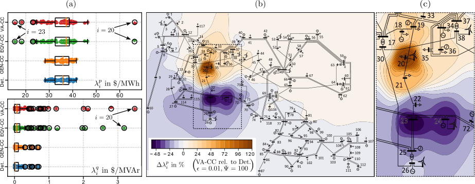
Also, increasing conservatism of the model increases system-wide balancing reserve price for both values of . For example, in the GEN-CC, the value of is only driven by chance constraints on power output limits of generators, as per Proposition 2, while the EQV-CC and VA-CC introduce additional components (e.g. reactive power, voltage and flow variances) to price as per Propositions 3 and 4. Location-specific prices and for all network nodes are displayed in Fig. 1a), while Figs. 1b)–c) map the relative difference between for the VA-CC case with and and the deterministic case. At the majority of nodes, prices (indicated by the box-plots in Fig. 1a) remain within 32–38 $/MWh. Note that unlike , which significantly increases for more conservative models, prices for and do not vary as much as conservatism increases. This corresponds to our findings in Propositions 1–4, which show that active and reactive power prices do not explicitly depend on the uncertainty and risk parameters. However, at some nodes, prices and in the GEN-CC and VA-CC cases exhibit larger deviations, e.g. see at nodes 20 and 23, which are also in proximity of wind farms, as shown in Fig. 1c). A resulting high flow variance on the line between nodes 19 and 23 causes price differentiation at nodes 19, 20, 21 and 23, 24, 25.
V-B Analysis of Variance of State Variables
Table I shows how the aggregated variance of state variables , , , change relative to the EQV-CC case as penalty increases. Even if is set to a small value, the variance of state variables reduce significantly, without a large increase in the objective function, expected generation cost, and prices and . Furthermore, as the value of increases, the relative reduction in variances of all state variables slightly reduces. The effect of variance penalty on prices is two-fold. First, it does not affect prices and relative to the EQV-CC case. Second, system-wide balancing price , which internalizes the variance penalties as per Proposition 4, increases with penalty .
VI Conclusion
This paper described an approach to internalize RES stochasticity and risk parameters in electricity prices. Using SOC duality, these risk- and variance-aware prices are derived from a chance-constrained AC-OPF and are itemized in terms of active and reactive power, voltage support and power flow components. We proved that active and reactive power prices do not explicitly depend on uncertainty and risk parameters, while expressions for balancing reserve prices explicitly include these parameters. Further, introducing variance penalties on the system state variables has been shown to internalize the trade-off between variance, risk and system cost at a modest increase in the expected operating cost. The results have been demonstrated and analyzed on the modified IEEE 118-node testbed. Future work includes extensions of the proposed market-clearing model to account for risk-averse strategies of market participants, enable risk trading instruments using our preliminary work in [27], and to account for multi-period trading horizons.
References
- [1] S. Sharma, “2019 methodology for determining minimum ancillary service requirements,” ERCOT, Tech. Rep., 2019. [Online]. Available: www.ercot.com/
- [2] NREL, “Western wind and solar integration study, national renewable energy,” Tech. Rep., 2010. [Online]. Available: www.nrel.gov
- [3] D. Bienstock, M. Chertkov, and S. Harnett, “Chance-constrained optimal power flow: Risk-aware network control under uncertainty,” Siam Review, vol. 56, no. 3, pp. 461–495, 2014.
- [4] M. Lubin, Y. Dvorkin, and S. Backhaus, “A robust approach to chance constrained optimal power flow with renewable generation,” IEEE Trans. Pwr. Sys., vol. 31, no. 5, pp. 3840–3849, 2016.
- [5] L. Roald et al., “Analytical reformulation of security constrained optimal power flow with probabilistic constraints,” in 2013 IEEE Grenoble Conference. IEEE, 2013, pp. 1–6.
- [6] W. Xie and S. Ahmed, “Distributionally robust chance constrained optimal power flow with renewables: A conic reformulation,” IEEE IEEE Trans. Pwr. Sys., vol. 33, no. 2, pp. 1860–1867, 2017.
- [7] M. Lubin, Y. Dvorkin, and L. Roald, “Chance constraints for improving the security of ac optimal power flow,” IEEE Trans. Power Syst., 2019.
- [8] L. Roald et al., “Corrective control to handle forecast uncertainty: A chance constrained optimal power flow,” IEEE Trans. Pwr. Sys., vol. 32, no. 2, pp. 1626–1637, 2016.
- [9] J. M. Morales et al., “Pricing electricity in pools with wind producers,” IEEE Trans. Pwr. Sys., vol. 27, no. 3, pp. 1366–1376, 2012.
- [10] J. Kazempour, P. Pinson, and B. F. Hobbs, “A stochastic market design with revenue adequacy and cost recovery by scenario: Benefits and costs,” IEEE Trans. Pwr. Sys., vol. 33, no. 4, pp. 3531–3545, 2018.
- [11] S. Wong and J. D. Fuller, “Pricing energy and reserves using stochastic optimization in an alternative electricity market,” IEEE Trans. Pwr. Sys., vol. 22, no. 2, pp. 631–638, 2007.
- [12] X. Kuang et al., “Pricing chance constraints in electricity markets,” IEEE Trans. Pwr. Sys., vol. 33, no. 4, pp. 4634–4636, 2018.
- [13] Y. Dvorkin, “A chance-constrained stochastic electricity market,” arXiv preprint arXiv:1906.06963, 2019.
- [14] F. C. Schweppe et al., Spot pricing of electricity. Springer Science & Business Media, 2013.
- [15] R. P. O’Neill et al., “Towards a complete real-time electricity market design,” Journal of Regulatory Econ., vol. 34, no. 3, pp. 220–250, 2008.
- [16] P. Lipka et al., “Running a more complete market with the slp-iv-acopf,” IEEE Trans. Pwr. Sys., vol. 32, no. 2, pp. 1139–1148, 2016.
- [17] D. Bienstock and A. Shukla, “Variance-aware optimal power flow,” in 2018 Power Sys. Comp. Conference (PSCC). IEEE, 2018, pp. 1–8.
- [18] E. Dall’Anese, K. Baker, and T. Summers, “Chance-constrained ac optimal power flow for distribution systems with renewables,” IEEE Trans. Pwr. Sys., vol. 32, no. 5, pp. 3427–3438, 2017.
- [19] A. J. Wood, B. F. Wollenberg, and G. B. Sheblé, Power generation, operation, and control. John Wiley & Sons, 2013.
- [20] R. Mieth and Y. Dvorkin, “Distribution electricity pricing under uncertainty,” arXiv preprint arXiv:1905.07526, 2019.
- [21] A. Ben-Tal and A. Nemirovski, Lectures on modern convex optimization: analysis, algorithms, and engineering applications. Siam, 2001, vol. 2.
- [22] S. S. Baghsorkhi and I. A. Hiskens, “Impact of wind power variability on sub-transmission networks,” in 2012 IEEE Power and Energy Society General Meeting. IEEE, 2012, pp. 1–7.
- [23] I. Dunning, J. Huchette, and M. Lubin, “JuMP: A modeling language for mathematical optimization,” SIAM Review, vol. 59, no. 2, 2017.
- [24] Code Supplement - AC CC-OPF Pricing. [Online]. Available: https://github.com/korpuskel91/acccopf_pricing
- [25] A. Wächter and L. T. Biegler, “On the implementation of an interior-point filter line-search algorithm,” Math. Prog., vol. 106, no. 1, 2006.
- [26] M. ApS, MOSEK.jl, 2019. [Online]. Available: https://github.com/JuliaOpt/Mosek.jl
- [27] R. Mieth, M. Roveto, and Y. Dvorkin, “Risk trading in a chance-constrained stochastic electricity market,” arXiv preprint arXiv:2003.01773, 2020.
Appendix A
Rewrite Equations 6–7 in the following form:
| (A.1) |
where the rows of matrices are equal to sensitivity vectors for and . First, we sort the rows of the terms in Equation A.1 by node types and introduce superscripts , , to indicate the node type:
| (A.2) |
where denote the blocks of re-arranged matrix from Equation A.1. Quantities are explicitly given by the uncertain generation and the respective system responses such that:
| (A.3) |
Notably, and are not part of the right-hand side of Equation A.3 because they are fixed parameters. Further, , , and as discussed in Section II-C. We use this relationship and Equations A.2–A.3 to compute the reactions of the uncontrolled variables to uncertainty :
| (A.4) |
Note that although implicitly depend on the AC power flow equations, these variables are endogenous to the model and not subject to uncertainty. Similarly, we get:
| (A.5) |
Using Equation A.4, we immediately obtain Equation 11 by separating matrix . Similarly, we obtain Equation 10 from separating matrix . In analogy, Equations 12–13 can be obtained by noting that and and combining the sensitivity factors respectively.