Analysis of Co-Occurrence Patterns in Data through Modular and Clan Decompositions of Gaifman GraphsThanks: This research was supported by European Research Council ERC-2014-CoG 648276 (AUTAR), by TIN2017-89244-R from Ministerio de Economia, Industria y Competitividad, and by Conacyt (México); we acknowledge recognition 2017SGR-856 (MACDA) from AGAUR (Generalitat de Catalunya).

José Luis Balcázar Affiliation: Universitat Politècnica de Catalunya Marie Ely Piceno

Abstract

We argue that the existing knowledge about modular decomposition of graphs and clan decomposition of 2-structures can be put to use advantageously in a context of data analysis. We show how to obtain visual descriptions of co-occurrence patterns by employing these decompositions on possibly generalized Gaifman graphs associated to datasets. We provide both theoretical advances that connect the proposed process to other data mining aspects (namely, closed set mining), as well as implemented algorithmics leading to an open-source tool that demonstrates our approach.

1 Introduction

We focus on two known concepts in the Theory of Computation, namely, modular decompositions and Gaifman graphs, as well as on a known generalization of modules, called clans. From a perspective of Data Analysis, modules and Gaifman graphs, taken together, have the potential of providing intuitive hierarchical depictions that explain data in interesting ways; also, some simple generalizations of Gaifman graphs may allow for clan decompositions and thus enhance that potential.

In order to motivate this work, we report briefly on one of the cases described in a previous conference submission [1]. We consider a simplified version of the famous dataset Titanic¹¹ 1 This variant, prepared by Radford Neal for the DELVE system, was downloaded from: http://www.cs.toronto.edu/ delve/data/titanic/desc.html where it is still available at the time of writing. [3]. For each of the 2201 people on board the well-known ship, this dataset records the values of four attributes: Traveling Class (first class, second class, third class, crew member), Sex (Female, Male), Age (discretized into Adult or Child) and Survival (Yes, No), that is, whether the person survived the sinking.

The modular decomposition via its standard Gaifman graph is shown in Figure 1. The meaning of each component of such a figure will be explained in depth along this paper, as it follows from the definition and properties of modules and Gaifman graphs; but, for the time being, we advance that each black dot represents a so-called “strong module”. Some of these are singletons, which consist of one value of one of the attributes, and the figure reflects it by linking the black dot to the explicitly given value. The others are nontrivial modules, represented by a box linked to the black dot.

Absence of a line connecting two dots means that no value below one dot co-occurs ever in the dataset with a value below the other: for instance, the two different values of each of the attributes Survival and Sex cannot occur together, so they remain disconnected.

On the other hand, a line connecting two dots means that every value below one of the dots co-occurs with every value below the other, somewhere in the dataset. For instance, the lower line in the triangle inside the top left box means that every combination of values of Sex and Survival appears in the dataset. The remainder of the triangle means that each of these four values, Yes, No, Male, Female, co-occurs somewhere with each and every one of the rest of the values: those of Age and Traveling Class.

The definition of module guarantees that no intermediate option exists between full connectivity and no connectivity: this is what makes this approach interesting. Our implemented, open-source system allows users to obtain such representations out of data with no particular interaction.

We focus now on the rightmost half of the figure. Like with Sex and Survival, one might expect a “box” (a module) with the four alternative values of the Traveling Class attribute, namely, 1st, 2nd, 3rd or Crew. Instead, we see that the value Crew “has migrated” to the parent box that includes the age values. This calls our attention to the following fact: whereas both adults and children appear in all the traveling classes, the crew included, of course, no children, at least as public records show; a fact that we might overlook in a non-systematic analysis and that is represented by the absence of a connecting line between Crew and Child. That is: even if the traveling class and the “Crew” label are employed as values in the same column, the data tells us, through our decomposition procedure, that they have different semantics. Additional discussion can be found in [1].

Refer to caption — Figure 1: Decomposing the standard Gaifman graph of the Titanic dataset.

Thus, these hierarchical depictions provide often easy-to-grasp explanations of co-occurrence patterns in the given data. Our team has shown also that, in a context of diagnostic data from medical practice in a cooperating hospital, the diagrams that we can obtain from our approach provide visual, interpretable hints about patterns of diagnostics that co-occur in the data [2], [14], [17].

The aim of this paper is twofold. We provide here a fundamental study of the process behind these applications, so as to better understand the processes we are applying; and also we develop a “systems” perspective, explaining the key implementation ideas employed in our open-source software tool to perform this sort of decomposition. Our theoretical study both supports our algorithmics and, also, explains how our approach relates to other existing data analysis options. Specifically, we explain how the modular decompositions of standard Gaifman graphs, and also the more general clan decompositions of some variants that we describe, fit a specific view of closure spaces that correspond to so-called “modular implications”, resp. “clan implications”, that we introduce here. This allows us to connect our approach with closure and implication mining, which are quite standard tools in Data Analysis.

Figure 2 shows us a general perspective of the intuitions behind our development. Both “vertical sequences” of processes are known; on one hand, from any graph, and thus for the so-called Gaifman graph that one can associate to a dataset, it is possible to determine its modules, filter the so-called strong modules, and organize them into the modular decomposition of the graph. In a similar way, we have that from a set of implications we can obtain closed sets and determine which of them are strong closures within the corresponding closure lattice: a well-known process.

Throughout this work we develop a theoretical framework that connects both processes: we show how to define the set of implications associated to a graph in such a way that strong modules and strong closures are the same sets. This connects intimately the modular decomposition with the closure lattice. As we move on to consider some extended, more quantitative analysis via generalized Gaifman graphs, we shall see that modules become insufficient and we adopt a known generalization, namely clan decompositions of symmetric 2-structures, for which we develop an analogous connection with closure lattices.

We are using different arrows for leftward / rightward connections in the top and bottom layers of Figure 2. At the top layer, given any graph, we demonstrate how to construct the modular implications, and how this process generalizes to clan implications; however, for the converse, not every implication set is valid, and it remains open to find intrinsic characterizations of sets of implications that correspond to a graph. Moreover, as we discuss below, the modular decomposition of a graph and of its complement are isomorphic and, accordingly, the modular implications do not distinguish between them.

Similarly, at the bottom layer, the closure space lattice determines the decomposition but, in the general case, it includes additional information; that is, the decomposition may not be sufficient to infer the whole closure space.

2 Preliminaries

Our work builds upon both the known connection between closure spaces and implications, and on several proposals for identifying hierarchical decompositions of graphs, namely, modules and, in a more general way, clans of 2-structures. However, the theory of 2-structures and their clans will be provided later on, after motivating the need of using them for certain generalizations of Gaifman graphs; initially, we will work with standard Gaifman graphs and we will only need modular decompositions. We explain these notions in this section.

2.1 Set-Theoretic Notations, Implications, and Closures

We assume that a given set $\mathcal{U}$ of potential items of interest has been fixed. Datasets will be assumed to come in transactional form, where each transaction is simply a subset of items. Set-theoretic notations are standard; $X\setminus Y$ denotes set difference: the elements of $X$ that do not appear in $Y$ . The complement of $X$ is $\mathcal{U}\setminus$ $X$ . Following customary usage, union is often denoted by mere juxtaposition, as in $XY$ .

Definition 1

Two sets $X$ and $Y$ overlap if the sets $X\cap Y$ , $X\setminus Y$ and $Y\setminus X$ are all three nonempty. Equivalently, $X$ and $Y$ do not overlap if and only if they are either disjoint, or a subset of one another.

Closure spaces on the powerset of the set of items will play an important role in our developments. A closure operator maps each set of items $X$ to a set of items, its “closure” $\overline{X}$ ; they are characterized by three properties:

•

Extensivity: $X\subseteq\overline{X}$
•

Idempotency: $\overline{\overline{X}}=\overline{X}$
•

Monotonicity: if $X\subseteq Y$ then $\overline{X}\subseteq\overline{Y}$

A set is a closed set if it coincides with its closure, and the closure space is the family of all the closed sets. A basic fact from the theory of closure spaces is that the intersection of closed sets is again closed.

Now we let items play the role of propositional variables. Then, implications are conjunctions of definite Horn clauses, where a set of clauses sharing the same antecedent are written as a single formula with conjunctions both at the antecedent and the consequent of an implication connective; we often write antecedents and consequents as mere sets, letting the conjunction connective implicit. For sets of items $X$ , $Y$ , and $Z$ , $Z$ satisfies the implication $X\Rightarrow Y$ , denoted as $Z\models X\Rightarrow Y$ , if either $X\not\subseteq Z$ or $XY\subseteq Z$ .

The fact, well-known in logic and knowledge representation, that Horn theories are exactly those closed under bitwise intersection of propositional models leads to a strong connection with closure spaces. It runs as follows: given a set of implications $\mathcal{B}$ , the closure $\overline{X}$ of a set $X$ is the largest set $Y$ such that $\mathcal{B}$ logically entails $X\Rightarrow Y$ ; whereas, if we are given a closure operator, we can axiomatize it by the set of implications $\{X\Rightarrow Y:X\subseteq\mathcal{U},Y\subseteq\overline{X}\}$ or, equivalently, any set of implications that entails exactly this set.

For references and supporting facts of all our claims so far, see the discussions in [19], [20] and [16] or its early version https://arxiv.org/abs/1411.6432v2.

Definition 2

$\overline{X}$ is a strong closure if, for all other closures $\overline{Y}$ , $\overline{X}$ and $\overline{Y}$ do not overlap. That is, either $\overline{X}$ and $\overline{Y}$ are disjoint, or are a subset of one another.

2.2 Modular Graph Decompositions

In many cases, items of $\mathcal{U}$ will be vertices of graphs in a fully standard way. Then, we use the terms “vertex” and “item” interchangeably. In all our graphs, we assume that no self-edge is ever present; also, we do not allow for multiple edges.

The modular decomposition of a graph is a process that consists of decomposing the graph into sets of vertices, nowadays called “modules”. It has been rediscovered many times and described under many different names [8], but the earliest appearance of the notion seems to be [7] ²² 2 An English translation is available as [10], where they are called “homogeneous sets”..

Definition 3

Given a graph, a set $X$ of vertices is a module if, for each vertex $y\notin X$ , either every member of $X$ is connected with $y$ or every member of $X$ is not connected with $y$ .

As modules can be proper subsets of other modules, we can obtain a hierarchical decomposition of the graph; these facts have been studied in a very wide bibliography (see [8] and the references there).

The modules of a graph can be seen, therefore, as subgraphs of the original graph. Note that the set of all vertices is vacuously a module, as are each vertex by itself and the empty set. These are called the trivial modules; we will systematically ignore the empty module.

As an intuition device that will become full-fledged in subsequent sections, we take the somewhat anthropomorphic stance of considering the presence or absence of an edge as the way one vertex “sees another”. Thus, we will often resort to expressions like “an item sees in a different way two other items” when it is connected to one of them and disconnected from the other one; or, in the same case, we may say that “the item can distinguish between two other items”. This intuition is customary in the field of 2-structures where the notion of a “clan”, a generalization of modules defined also below in Section 4, relies on this intuitive device.

Hence, throughout this paper, the presence or absence of edges will convey only the idea of two different ways one item sees another; that is, we give the same interpretation to a graph and to its complement. Indeed, permuting absence and presence of all edges does not change the ways vertices distinguish each other. Thus, we may state the following proposition:

Proposition 1

A graph and its complement leave the same set of modules, therefore, the same modular decomposition.

On the basis of the definition of module, we can state (see [8]):

Proposition 2

Consider a graph and the modules in it.

1.

Let $x$ and $y$ be elements of a module $\mathcal{M}$ : if vertex $z$ is connected to exactly one of $x$ and $y$ then, necessarily, $z\in\mathcal{M}$ .
2.

Let sets $X$ and $Y$ be non-disjoint: $X\cap Y\neq\emptyset$ . If both are modules, then also $X\cap Y$ , $X\setminus Y$ , and $Y\setminus X$ are modules.
3.

Let sets $X$ and $Y$ be disjoint. If both are modules, then either every $x\in X$ is connected to every $y\in Y$ , or no $x\in X$ is connected to any $y\in Y$ .

This last statement was already announced informally in our Introduction. It leads to a main interest of the notion of module, namely, all the vertices of a module can be collapsed into a single vertex without ambiguity with respect to how to connect it to the rest of the vertices: the new vertex gets connected to $y$ if all the members of the module were connected to $y$ , and remains disconnected if all the members were disconnected. Clearly, the definition given of module is what is needed for this process to be applied without ambiguity about whether the new vertex should or should not be connected to some external vertex $y$ . More generally, the same considerations apply if we simultaneously collapse into single vertices two disjoint modules: either they are connected, in the sense that all the respective pairs of vertices (one from each module) are, or they are not because no such pair is.

Nothing forbids modules to intersect each other; in that case, though, collapsing one module into a single vertex may affect the other. In order to avoid side effects, it is customary to restrict oneself to so-called “strong modules” [7] (see also [10]): they allow us to obtain a tree-like decomposition.

Definition 4

A module $\mathcal{M}$ is a strong module of a graph if it does not overlap any other module; that is, for all other modules of the graph $\mathcal{M}^{\prime}$ , either $\mathcal{M}\cap\mathcal{M}^{\prime}=\emptyset$ or they are subsets of one another.

Given a graph, we can focus on its maximal strong modules; it is known that each vertex belongs to exactly one of them [8]. Thus, one, or more, or even all of these maximal strong modules can be collapsed into a single vertex each. The resulting graph is called as “quotient graph”.

Definition 5

Given a graph, its coarsest quotient graph is obtained by collapsing into respective vertices all its maximal strong modules.

Then, a tree-like structure arises from the fact that each of these modules, taken as a set of vertices, is actually a subgraph that can be recursively decomposed, in turn, into maximal strong modules, thus generating views of subsequent internal structures given by their respective coarsest quotient graphs. We display the decomposition tree while labeling each node (a strong module) with the corresponding coarsest quotient graph, and connect visually each collapsed vertex to the subtree decomposing the corresponding module. Of course, the root of the “tree” is the coarsest quotient of the whole graph.

Example 1

Figure 3 shows a simple example of modular decomposition. It is easy to check that $\{a,b,c\}$ conforms a module: both $d$ and $e$ are connected to each of them. The other possible nontrivial modules are $\{a,b,c,d\}$ , $\{a,b,c,e\}$ , $\{d,e\}$ , $\{a,b\}$ , $\{a,c\}$ , and $\{b,c\}$ ; they are not strong: each of them intersects others. Instead, $\{a,b,c\}$ is a strong module as it does not overlap any other module. The root is the fully connected coarsest quotient graph where $\{a,b,c\}$ , the single nontrivial maximal strong module, has been collapsed to a single vertex. Each of the three vertices is connected to the module they represent: two are maximal strong but trivial ones, and the largest one decomposes itself again into three trivial modules.

Of course, Figure 1 is also an example of modular decomposition, to which we will return later on, and further examples will keep appearing throughout the paper.

2.3 Gaifman Graphs

Gaifman graphs are mathematical structures introduced several decades ago as a means to study limitations of the expressivity of logical languages [9]. They are defined on first order relational structures (that is, in essence, relational databases) and their basic notion is pretty simple:

Definition 6

Given a first order relational structure $\{R_{i}\}_{i\in I}$ where the values appearing in the tuples of the relations $R_{i}$ come from a fixed universe $\mathcal{U}$ , its corresponding Gaifman graph has the elements of $\mathcal{U}$ as vertices, and each edge $(x,y)$ , for $x\neq y$ , is present in the graph exactly when $x$ and $y$ appear together in some tuple $t\in R_{i}$ , for some $R_{i}$ .

We extend this notion in various ways along this paper. Labeled versions will be introduced below in Section 5; for the time being, we only remark that the notion extends naturally into transactional data: for each transaction, and for each pair of different items $x$ and $y$ in that transaction, we ensure that the edge $(x,y)$ is present in the graph, and that only such edges are.

It is, of course, possible to apply the modular decomposition method on this sort of graph. In reference to the data on which the graph was constructed: what can be said of the obtained decomposition, in terms of data analysis? This paper belongs to a line of research based on this question.

3 A Closure-Based View of Modules

We start with the top, left-to-right arrow of Figure 2: given a graph, we show how it is possible to describe the conditions for a subgraph being a module in the form of a set of implications. This leads to connections between tree-like modular decompositions, as described above, and the theory of closure spaces. We show first how to obtain these implications, and then discuss some of the resulting connections.

Indeed, the implicational view is already implicit in Proposition 2 (1): if $x$ and $y$ are elements of any module $\mathcal{M}$ and $z$ sees them in a different way, then $z\in\mathcal{M}$ . With the standard semantics of implications, taking again vertices (items) as propositional variables and, hence, subgraphs as models, this is equivalent to: $\mathcal{M}\models xy\Rightarrow z$ .

To pursue this idea further, given a graph, we generate a set of implications from it; we call this set the set of “modular implications” of the graph. In each implication, the antecedent will be a pair of vertices in the graph, and the consequent will be conformed by those vertices that see the vertices in the left side in different ways.

Formally, we need to establish some notation. Given a graph $\mathcal{G}$ and a vertex $x$ in it, we denote by $\mathcal{N}_{\mathcal{G}}(x)$ the set of immediate neighbors of $x$ in $\mathcal{G}$ , and define the “distinguishing set” of a pair of vertices $x$ , $y$ , as follows:

\mathcal{D}_{\mathcal{G}}(x,y)=(\mathcal{N}_{\mathcal{G}}(x)\setminus\mathcal{N}_{\mathcal{G}}(y))\cup(\mathcal{N}_{\mathcal{G}}(y)\setminus\mathcal{N}_{\mathcal{G}}(x))\setminus\{x,y\}.

That is, this set gathers together all the vertices that see one given pair in different ways. Note that it is necessary to remove explicitly $x$ and $y$ from the distinguishing set. Indeed, in case they are connected, the absence of self-edges would make each of them qualify to distinguish themselves from the other, whereas the definition of module only searches for distinguishing vertices outside the module. Then, we construct the set of modular implications as follows:

Definition 7

For graph $\mathcal{G}$ and different vertices $x$ , $y$ in it, the corresponding modular implication is $xy\Rightarrow\mathcal{D}_{\mathcal{G}}(x,y)$ . The set of modular implications for $\mathcal{G}$ is formed by the modular implications corresponding to every pair of different vertices, for which the right-hand side is nonempty: $\mathcal{D}_{\mathcal{G}}(x,y)\neq\emptyset$ .

We can state the following:

Proposition 3

For graph $\mathcal{G}$ and different vertices $x$ , $y$ in it, in the corresponding modular implication $xy\Rightarrow Z$ we have $z\in Z$ if and only if $z\notin\{x,y\}$ and $z$ is connected to exactly one of $x$ , $y$ . Therefore, $\{x,y\}$ is a module (of size 2) if and only if $Z=\emptyset$ .

The proof is direct from the definition of module.

Example 2

Let us continue the previous example by showing the set of modular implications from the same graph and the corresponding closure space. From Figure 3 we obtain the following set of modular implications:

$ad\Rightarrow bc$

$ae\Rightarrow bc$

$bd\Rightarrow ac$

$be\Rightarrow ac$

$cd\Rightarrow ab$

$ce\Rightarrow ab$

The pairs $\{a,b\}$ , $\{a,c\}$ , $\{b,c\}$ , $\{d,e\}$ , are size-2 modules and would lead to empty right-hand sides in their modular implications; accordingly, these implications are discarded.

In the left side of Figure 4 we find the closure space lattice described by the modular implications obtained from the graph. For convenience in the comparison, we display again at the right the decomposition from Figure 3, and we mark in bold those closed sets that do not overlap any other closed set (strong closures as per Definition 2).

The main result of this section is Theorem 3.1.

Theorem 3.1

The modules of a graph and the closures defined by its set of modular implications are the same sets.

Proof

(Closures are modules.) Let $X$ be a closure, and suppose that there is some $y$ that can distinguish two arbitrary $x_{1},x_{2}\in X$ ; one of the modular implications will be $x_{1}x_{2}\Rightarrow Y$ with $y\in Y\neq\emptyset$ . As $X$ is a closure, it must satisfy all the modular implications, and both antecedents are in $X$ , thus $y\in X$ . Hence, no $y$ outside $X$ may distinguish two elements inside $X$ , which is the definition of module.

(Modules are closures.) Let $X$ be a module. It suffices to show that it satisfies all the modular implications: let $x_{1}x_{2}\Rightarrow Y$ be one of them. If either $x_{1}\notin X$ or $x_{2}\notin X$ , then $X$ satisfies the implication by failing the antecedent. If $x_{1},x_{2}\in X$ then, since $X$ is a module, no item outside $X$ can distinguish them; but, according to Proposition 3, $Y$ is the set of items that distinguish them, hence $Y\subseteq X$ and $X$ satisfies the modular implication.

Corollary 1

Strong modules and strong closures are the same sets.

Thus, the match seen in Figure 4 is not chance. The closures that are not strong do correspond exactly to the additional modules described at the end of Example 1. In the following, and until explicitly indicated otherwise, whenever we talk about closures, we are refering to the closures described by the set of modular implications.

3.1 Graph Reconstruction

This section develops the reverse arrow at the top of Figure 2: from the set of modular implications of a graph $\mathcal{G}$ defined on the vertices $\mathcal{U}$ $=\{v_{1},\ldots,v_{n}\}$ , it is possible to construct a graph $\mathcal{G}_{a}$ with exactly the same decomposition, taking just those implications whose left parts are in the form $v_{1}v_{2},\ldots,v_{n-1}v_{n}$ . The graph is either $\mathcal{G}$ or its complement because, following Proposition1, they have the same set of modules and essentially the same modular decomposition. The idea to reconstruct the graph is to take from the set of implications a smaller number of well-chosen implications; we show that they give us enough information about the relations between the edges to be able to reconstruct the graph.

Algorithm 1 Construction of a connex graph

\mathcal{G}^{\prime}

on the set of vertices determined by the edges of a graph

\mathcal{G}

Input: Set of modular implications of

\mathcal{G}

Output:

\mathcal{G}^{\prime}=(\mathcal{U}_{\mathcal{G}^{\prime}}

\mathcal{E}_{\mathcal{G}^{\prime}})

, with binary labeling on its edges.

Let

\mathcal{U}_{\mathcal{G}^{\prime}}

be an empty set.

Let

\mathcal{E}_{\mathcal{G}^{\prime}}

be an empty set.

for all

j=\overline{2,n}

Add

v_{1}v_{j}

\mathcal{U}_{\mathcal{G}^{\prime}}

2<j

then

Add

(v_{1}v_{j-1},v_{1}v_{j})

\mathcal{E}_{\mathcal{G}^{\prime}}

in the following way

v_{1}\in Z

, such that

v_{j-1}v_{j}\Rightarrow Z

then

(v_{1}v_{j-1},v_{1}v_{j})=0

else

(v_{1}v_{j-1},v_{1}v_{j})=1

end if

for all

i=\overline{2,j-1}

Add

v_{i}v_{j}

\mathcal{U}_{\mathcal{G}^{\prime}}

Add

(v_{i-1}v_{j},v_{i}v_{j})

\mathcal{E}_{\mathcal{G}^{\prime}}

in the following way

v_{j}\in Z

, such that

v_{i-1}v_{i}\Rightarrow Z

then

(v_{i-1}v_{j},v_{i}v_{j})=0

else

(v_{i-1}v_{j},v_{i}v_{j})=1

end if

end for

end if

end for

Before explaining our algorithm to reconstruct the graph we have the following propositions.

Proposition 4

Let $Z=\mathcal{D}_{\mathcal{G}}(x,y)$ , if we have the module implications $xy\Rightarrow Z$ we know $(x,z)\neq(y,z)$ for all $z\in Z$ . Also we know, $(x,w)=(y,w)$ for all $w\in\mathcal{U}\setminus$ $Z$

The implications will tell us only which vertices distinguish other vertices. Even if we know that vertex $z$ distinguishes $x$ ftom $y$ , this only tells us that $z$ is connected to exactly one of the other two, but we do not know which one. We can choose one of them, but then the choice influences the presence or absence of other edges.

Algorithm 2 Constructing the path that connects two vertices

v_{l}v_{k}

and

v_{m}v_{p}

in the graph

\mathcal{G}^{\prime}=(\mathcal{U}_{\mathcal{G}^{\prime}}

\mathcal{E}_{\mathcal{G}^{\prime}})

Input: Two vertices

v_{l}v_{k}\in\mathcal{U}_{\mathcal{G}^{\prime}}

and

v_{m}v_{p}\in\mathcal{U}_{\mathcal{G}^{\prime}}

, where

k\leq p

, without losing generality.

Output: The set of vertices that conform the path that connects the vertices

v_{l}v_{k}

and

v_{m}v_{p}

Let

Path

be an empty set

k==p

then

l<m

then

for all

i=l

m

Add

v_{i}v_{p}

Path

end for

else

for all

i=m

l

Add

v_{i}v_{p}

Path

end for

end if

else

for all

i=l

1

Add

v_{i}v_{k}

Path

end for

for all

i=k+1

p

Add

v_{1}v_{i}

Path

end for

for all

i=2

m

Add

v_{i}v_{p}

Path

end for

end if

Return

Path

The way through will be to construct a larger but sparse connex graph $\mathcal{G}^{\prime}$ using the Algorithm 1, whose vertices are all possible edges from the graph $\mathcal{G}$ and the edges determine the relation between these edges: either one exists in $\mathcal{G}$ and the other does not, or both are equal in this respect (either by existing both or none of them). As the graph $\mathcal{G}^{\prime}$ is a connex graph, once a type of edge is assigned to any single edge, we may deduce the type for all the remaining edges and construct the graph $\mathcal{G}_{a}$ . We find that the order of the edges in the graph $\mathcal{G}^{\prime}$ is related to the first two levels of the SE-tree [18].

For the Algorithm 1, it is possible to determine when two edges get different status by following the Proposition 4: two given edges, $v_{i}v_{k}$ and $v_{j}v_{k}$ of $\mathcal{G}$ , are in different status if for the implication $v_{i}v_{j}\Rightarrow Z$ , $v_{k}\in Z$ . Whether we know that two edges are in the same status, or in different ones, as soon as we can determine whether one of them is an edge of $\mathcal{G}$ the other gets determined as well.

The Algorithm 1 constructs a connex graph since given two vertices on it there is a path that connects them, the Algorithm 2 gives us this path. In fact, the length of the path that connects the edge $v_{l}v_{k}$ to $v_{m}v_{p}$ is $(l-1)+(p-k)+(m-1)$ where $p>k$ , while if $p=k$ , the length of the path is $|l-m|$ .

Example 3

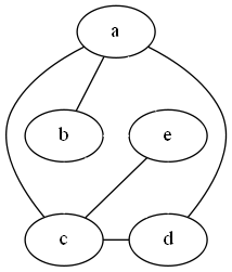
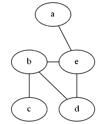
Let us apply the Algorithm 1 on the following set of implications obtained from the graph of Figure 5:

$ab\Rightarrow cd$

$ac\Rightarrow be$

$ad\Rightarrow b$

$ae\Rightarrow bd$

$bc\Rightarrow de$

$bd\Rightarrow c$

$be\Rightarrow ac$

$cd\Rightarrow e$

$ce\Rightarrow ad$

$de\Rightarrow a$

Thus, Algorithm 1 leads to the connex graph $\mathcal{G}^{\prime}=(\mathcal{U}_{\mathcal{G}^{\prime}}$ , $\mathcal{E}_{\mathcal{G}^{\prime}})$ , where $\mathcal{U}_{\mathcal{G}^{\prime}}$ $=\{ab,ac,bc,ad,bd,cd,ae,be,ce,de\}$ , as displayed in Figure 6. A label 1 joining two vertices of $\mathcal{G}^{\prime}$ means that both of the corresponding edges of $\mathcal{G}$ must be in equal status: either both are present or both are absent in $\mathcal{G}$ . A label 0, instead, means that they must have different status: exactly one of them exists in $\mathcal{G}$ .

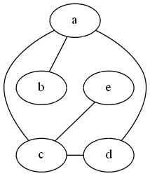
The possible reconstructed graphs are shown in Figure 7. It remains to decide on one edge, such as the initial vertex of $\mathcal{G}^{\prime}$ corresponding to $(a,b)$ .

So, suppose the edge $(a,b)$ exists, that is $a$ and $b$ are connected. As we may see in Figure 6 $(a,c)$ and $(a,d)$ are in the same status as $(a,b)$ , while $(b,c)$ is not, thus $b$ and $c$ are disconnected, and $a$ is connected with $c$ and $d$ . We also know that $(a,d)$ is in different status than $(a,e)$ and $(b,d)$ , thus $a$ and $e$ are disconnected, and also, $b$ and $d$ are disconnected. We know $(b,d)$ and $(c,d)$ are in different status, thus, $c$ and $d$ are connected; while $(a,e)$ is in the same status as $(b,e)$ , thus, $b$ and $e$ are disconnected. Also, we have that $(b,e)$ is different from $(c,e)$ , meaning that $c$ and $e$ are connected. At the same time $(c,e)$ is different from $(d,e)$ , thus $d$ and $e$ are disconnected. In this way we get the graph in the left of Figure 7.

If we had started by choosing that the edge $(a,b)$ does not exist, following the constraints describe in Figure 6, we get the graph in the right of Figure 7 which is, of course, the complement graph and has the same set of modular implications by Proposition 1.

3.2 Module Taxonomy

To maintain consistency within the paper, for some notions we will be using terminology corresponding to the theory of 2-structures [6] instead of the classical terms in modular decompositions. A graph of three or more vertices is called primitive if all of its modules are trivial, while if either all of its vertices are connected, or all of its vertices are disconnected, we say that it is complete; in this case, every subset is a module and there are no strong nontrivial modules. By convention, graphs of size 1 or 2 are considered complete. In fact, it can be seen easily by exhaustive inspection that at least 4 vertices are necessary for primitive graphs.

Modules can be primitive or complete themselves as well. The qualifier is customarily chosen according to their corresponding coarsest quotient graphs (Definition 5), and not according to themselves as subgraphs. Indeed, these terms are most often applied to coarsest quotient graphs, such as those labeling the nodes of a tree decomposition. Specifically, it is a theorem of modular decomposition that the coarsest quotient graphs labeling each node of a decomposition tree, if nontrivial, are all either primitive or complete. Graphs whose tree does not show any primitive quotient graph are called “cographs” and have a large number of graph-theoretic and algorithmic properties. The graph $P_{4}$ is the path on 4 vertices with 3 edges; its complement is also $P_{4}$ , and plays a key role in modular decompositions, as follows:

Proposition 5

Primitive graphs (and thus also their complements) always have induced $P_{4}$ subgraphs [15]³³ 3 See also https://en.wikipedia.org/wiki/Cograph and the references there.. Hence, for a primitive module, its corresponding coarsest quotient graph consists of at least four maximal strong modules.

As an example, both nonsingleton quotient graphs in Figure 3 are complete, even if the graph itself is not, whereas in Figure 1 we can see a primitive coarsest quotient that coincides, actually, with $P_{4}$ . We show below one example where only primitive modules appear in the decomposition.

Among other terms, primitive modules are sometimes called neighborhood modules. Modular decomposition theory distinguishes fully disconnected complete graphs (or “parallel” modules) and fully connected ones (or “series” modules), leading to often duplicated arguments and definitions because both cases fulfill the same role. Indeed, recall from Proposition 1 that presence or absence of edges can be swapped with no change in the modular structure: that’s why fully connected and fully disconnected modules are treated similarly. Hence, we prefer the view, originated in the study of 2-structures, of naming them both “complete” [6] (see below).

3.3 Closures and Module Types

By Theorem 3.1 and Corollary 1 we have that modules and closures, strong or not, are the same sets, this relation is represented in the Figure 2 by the double arrows. As we shall see below, the strong modules and their types will be important in the visualization of co-occurrence patterns in data analysis. Thus, we would like to be able to get the type of a strong module, that is, whether the module is complete or primitive, by using just the information in the closure lattice.

Following this idea we show, in this section, that the type of a strong module is given by the immediate closure subsets of its respective strong closure; in this way, we may go from the modular decomposition of a graph to the closure space lattice, and viceversa, as the arrows at the end of our scheme in the Figure 2 indicate.

The immediate closure subsets of a set $X$ are the children of $X$ in the closure lattice: namely, closed (not necessarily strong) subsets $Y$ of $X$ such that no intermediate set $Z$ , $Y\subset Z\subset X$ , is closed.

Theorem 3.2

The type of the coarsest quotient graph of a module is primitive if and only if the immediate closure subsets of its corresponding closure in the closure lattice are strong closures and they are more than three.

Proof

Let $\mathcal{M}$ be a module; by Corollary 1 its corresponding closure in the closure lattice is also $\mathcal{M}$ , and let us suppose that its coarsest quotient graph collapses the maximal strong modules $\mathcal{M}_{i}$ ( $i\in I$ for some index set $I$ ).

( $\Rightarrow$ ) Let $\mathcal{M}$ be a primitive module, that is its corresponding coarsest quotient graph is primitive; we have to prove that there is not any union of $\mathcal{M}_{i}$ ’s closure subset $\mathcal{F}$ such that $\mathcal{M}_{i}\subset\mathcal{F}\subset\mathcal{M}$ . $\mathcal{F}$ must be a union of $\mathcal{M}_{i}$ since, by the premise, $\mathcal{M}_{i}$ are strong closures so $\mathcal{F}$ does not overlap any of them.

But if $\mathcal{F}$ includes at least two $\mathcal{M}_{i}$ , by definition of primitive there must be at least one other $\mathcal{M}_{i}$ distinguishing them; thus $\mathcal{F}$ could not be a closure.

( $\Leftarrow$ ) We have to prove that if the immediate closures $\mathcal{M}_{i}$ of a strong closure $\mathcal{M}$ are strong closures and more than three, then $\mathcal{M}$ is a primitive module. Let $J\subset I$ be the index set of a proper subset of the modules $\mathcal{M}_{i}$ , consisting of at least two of them (we can guarantee this possibility by the premise). Suppose that all the remaining $\mathcal{M}_{i}$ ’s, $i\notin J$ , cannot distinguish between them, so $\bigcup_{j\in J}\mathcal{M}_{j}$ must be a closure; this would contradict the fact that all the $\mathcal{M}_{i}$ ’s are immediate closed subsets of $\mathcal{M}$ . Thus, for arbitrary $J\subset I$ , there must be at least one $\mathcal{M}_{i}$ , $i\notin J$ , that may distinguish between some of them so that no such $\bigcup_{j\in J}\mathcal{M}_{j}$ is a module. Subsets that are not in the form $\bigcup_{j\in J}\mathcal{M}_{j}$ are not modules either because each $M_{i}$ being a strong module means that no module overlaps any of them. Thus, $\mathcal{M}$ is a primitive module.

Let us see some examples to illustrate both cases.

Example 4

In Figure 8 (left) there is a graph with primitive quotient graphs in its decomposition. We get from it the following set of modular implications:

$ab\Rightarrow c$

$ac\Rightarrow d$

$ad\Rightarrow bc$

$ae\Rightarrow cdf$

$af\Rightarrow bg$

$ag\Rightarrow bef$

$bc\Rightarrow ad$

$bd\Rightarrow a$

$be\Rightarrow df$

$bf\Rightarrow acg$

$bg\Rightarrow acef$

$cd\Rightarrow b$

$ce\Rightarrow af$

$cf\Rightarrow bdg$

$cg\Rightarrow bdef$

$de\Rightarrow abf$

$df\Rightarrow cg$

$dg\Rightarrow cef$

$ef\Rightarrow abcdg$

$eg\Rightarrow abcd$

$fg\Rightarrow e$

This implication set generates the closure lattice in the center of Figure 8. The nodes $abcdefg$ and $abcd$ have four strong closures as children, and indeed their equivalent strong modules into the decomposition are primitive as Theorem 3.2 says.

Example 5

In Figure 9 there is an example of a graph with only complete quotient graphs in its decomposition. From Figure 9 left we get the set of modular implications:

$ac\Rightarrow b$

$ad\Rightarrow ce$

$ae\Rightarrow b$

$bc\Rightarrow a$

$bd\Rightarrow ce$

$be\Rightarrow a$

$cd\Rightarrow abe$

$de\Rightarrow abc$

with $ab$ and $ce$ closed sets.

At the center of Figure 9 we have the closure lattice from this set of implications. As we can see, the closed set $abcde$ has two children so its respective quotient graph in the decomposition is a complete module. The closed set $abce$ has three children overlapping, by the Theorem 3.2, we may deduce its respective coarsest quotient graph in the decomposition is complete as we can see in the Figure 9 right. The last closed set in the closure lattice is $ab$ , it has two children so its respective quotient graph is a complete module as we may see in the decomposition tree.

3.4 Data Analysis via Gaifman Graph Decomposition

We will return below to a more general approach for these sort of decompositions. However, we find it is high time to pause the theoretical development and motivate, with some example tasks of data analysis, what we have presented so far in more detail than the mere hints given in the Introduction. For a given relational dataset, we take all values of the attributes (possibly including an indication of the intended attribute) as items into a transactional view and, hence, as vertices of a Gaifman graph. Then, by definition, it represents information about item co-occurrences in the dataset, since edges $(x,y)$ , for $x\neq y$ , exist when the items $x$ and $y$ appear together in some tuple. Despite its multirelational potential, to be explored in future work, we restrict ourselves to Gaifman graphs of single tables, which is sufficient for the commonly employed benchmark datasets. Then, the modular decomposition groups the vertices in the hierarchical way that we have seen.

Let us start by going back to the modular decomposition of the standard Gaifman graph of the Titanic dataset that we have described in the Introduction (Figure 1). The modules for sex and survival are clear and intuitive: as they are different possible values for the same attribute, they never appear together, but happen to have the same set of neighbors⁴⁴ 4 Vertices with the same set of neighbors are commonly called “twins” in graph theory: “true twins” if they are connected and “false twins” otherwise, like here; we will see often such cases in our examples because the same set of neighbors implies that they form a size-2 module.. We did already explain why the top module is fully connected: a complete coarsest quotient of the whole graph; we also pointed out how the lack of children among the crew results in the vertex for Crew moving away from the other values of the same attribute and into the “age” module, thus showing the semantic difference with the traveling classes. The coarsest quotient of this module collapses the traveling classes into a single vertex and, together with the other three trivial clans, creates a size-4 primitive module that, by Proposition 5, cannot be anything else but $P_{4}$ . Further related discussions are given in [1].

Now, we describe some outcomes of analysis on the well-known dataset Mushroom, also known as “Agaricus - Lepiota”. There, a number of purported attributes of potential mushrooms of these families are expected to be useful to predict whether each of the 8124 observations would correspond to an edible or a poisonous mushroom [5]. (The data was compiled by mushroom experts out of hypothetical mushroom observations, not actual ones.)

Often, in practice, graphs may have large amounts of vertices. Here and also later, with other datasets, we choose to work with those vertices that appear in the transactions more frequently than some determined threshold. In order to get understandable, smallish but representative diagrams; we restrict ourselves to the $n$ most frequent items, for a reasonable value of $n$ that leads to understandable diagrams. Specifically, for Mushroom, we restrict ourselves first to items appearing at least 2000 times.

Even then, we discuss some of its modules but do not display the complete decomposition tree, because the space is not enough to show it adequately; for instance, we obtained as a root of the tree decomposition a complete node with many singleton items. Also, of course, a number of false twins appear, such as grass-living versus wood-living mushrooms, obviously disconnected. Then, there are also a few interesting modules. First, again a $P_{4}$ case is shown in Figure 10: if a mushroom has foul odor, then it is a poisonous mushroom, as “foul odor” never appears in the same tuple with “edible” (and again the three missing edges are also a $P_{4}$ ).

Figure 11 is a little bit more difficult to interpret but we find there, for example, that bruised mushrooms have smooth stalk surfaces, both below and above, but never exhibit silky surfaces either below or above, and not all smooth stalk surfaces, either below or above, are bruised, since both are also connected to the no-bruises vertex. The induced $P_{4}$ predicted by the theory is indeed there as well (but somewhat more difficult to pinpoint).

The reader can find further modular decomposition of other datasets in our previous papers [1] and [2].

3.5 Decomposing Thresholded Gaifman Graphs

Now we consider an alternative way to handle datasets via a variant of Gaifman graph. Sometimes, we may be interested in keeping track of quantitative information that the standard Gaifman graph lacks. Perhaps the simplest alternative variant of Gaifman graph for this purpose is the thresholded Gaifman graph [1] (other alternatives are discussed below in Section 5.2). In this variant, the difference in the edges, instead of being zero joint occurrences versus 1 or more, resorts to a threshold possibly different from 1: those pairs of items that appear together less often than the determined threshold are considered as “not frequent enough” and remain disconnected, whereas connections represent frequencies of co-occurrence higher than or equal to the threshold.

Often, we will apply an additional visual simplification. With larger datasets, the usual outcome of the analysis includes mostly large primitive modules of unclear interpretability. The diagram may become, then, uninteresting. In order to construct helpful visualizations, we encompass uninteresting substructures into single nodes that we label “Others”, as we will do next. Two very common cases are, first, large sets of fully disconnected vertices and, second, large, complicated primitive modules that do not convey intuitive information.

A first example from [1]: for the same version of the Titanic dataset described above, assume that we wish to ignore co-occurrences of pairs of items if they occur together less than 1000 times. In the thresholded Gaifman graph, such pairs of items will be kept disconnected. The resulting decomposition tree for that Gaifman graph (slightly simplified by grouping as Others the rest of the fully disconnected vertices as just indicated) is shown in Figure 12. In a sense, this image displays the well-known saying: “women and children first”.

Working instead with the Mushroom dataset, with attributes appearing more than 2000 times and considering as not frequent enough those co-occurrences below 1000 times we obtain the decomposition shown in Figure 13, where we see a handful of very frequent items that co-occur with each other. Naturally, we might like to see more detailed information: in this case, one way to decompose the node Others is to give a lower threshold. Giving 800 as threshold value we may see part of the internal behavior of the Others node; the Figure 14 show this part of the decomposition. For this example, we have that there are more than 800 mushrooms but less than 1000 that are edible and do not have odor, and also there is a similar quantity of mushrooms whose ring stalk surfaces, above and below, are silky.

4 2-structures and clan decomposition

The notion of modular decomposition is enough to be applied on standard or thresholded Gaifman graphs, but is insufficient to handle adequately other variations of Gaifman graphs that we will want to study as well; for the rest of this paper, we will work with a more general notion, namely, 2-structures and their clans [6].

Definition 8

A 2-structure is a complete graph, endowed with an equivalence relation among its edges.

In specific, we work only with the so called symmetric 2-structures [6] where all the equivalence classes are symmetric. An equivalence class $\mathcal{E}_{i}$ on a set $\mathcal{U}$ is symmetric if for all $x,y\in\mathcal{U}$ : $(x,y)\in\mathcal{E}_{i}\Leftrightarrow(y,x)\in\mathcal{E}_{i}$ . Since in the 2-structures that we use the edges represent co-occurrences, is the same to say that $y$ co-occurs with $x$ than $x$ co-occurs with $y$ . Then, our equivalence classes of co-occurrences will always be symmetric equivalence classes. Hence, all along this paper, whenever we talk about 2-structures, we will be referring to symmetric 2-structures.

It is possible to see a Gaifman graph as a 2-structure where all the absent edges will be in the same equivalence class while the existing edges will belong to the other equivalence class. In this way we get a complete graph with two equivalence classes. In a similar way, thresholded Gaifman graphs also can be seen as 2-structures with two equivalence classes. Actually, the general form of 2-structures would be akin to directed graphs and, as Gaifman graphs and their generalizations are instead undirected, symmetric 2-structures suffice.

This view is also consistent with the claim that in the field of modular decompositions, the crucial notion is not presence or absence of an edge, but the difference between them. In this sense, a graph and its complement correspond, in fact, to the same 2-structure. The advantage of working with 2-structures is that they allow us to work with more than two equivalence classes. Then, the decomposition procedure is based, instead of modules, on the so-called “clans”. They extend the intuitive concept of when a vertex sees in different ways two vertices. In 2-structures we say that an item $x$ “sees in a different way” two other items if the edges that connect $x$ with these two items are not equivalent. That is, $x$ sees in a different way $y$ and $z$ if the edges $(x,y)$ and $(x,z)$ lie in different equivalence classes. Alternatively, we say $x$ can distinguish between $y$ and $z$ . Note that this is consistent with the previous usage when a graph is seen as a 2-structure with two equivalence classes.

Thus the notion now corresponding to “module” has been called always a “clan”. For a 2-structure given by a set of vertices $\mathcal{U}$ and an equivalence relation $\mathcal{E}$ on its edges, we say that the subset $X\subseteq\mathcal{U}$ is a clan, informally, if, for every $y\in\mathcal{U}$ $\setminus X$ , $y$ cannot distinguish the elements of $X$ . Formally [6]:

Definition 9

Given $\mathcal{U}$ and an equivalence relation $\mathcal{E}\subseteq((\mathcal{U}\times\mathcal{U})\times(\mathcal{U}\times\mathcal{U}))$ on the edges of the complete graph on $\mathcal{U}$ , $C\subseteq\mathcal{U}$ is a clan when

\forall x\notin C\,\forall y\in C\,\forall z\in C\,((x,y),(x,z))\in\mathcal{E}.

Thus, two members of a clan cannot be distinguished by anyone outside the clan, an idea that motivated the choice of the term. As with the trivial modules, the so called trivial clans are all the singletons $\{x\}$ for $x\in\mathcal{U}$ , as well as $\mathcal{U}$ itself and the empty set. When we see a graph as a 2-structure, as indicated above, its clans are the modules. Of course the clans can be again of two types, complete or primitive, like the modules: in a primitive clan, there are no nontrivial clans; in a complete clan, all edges are equivalent. In order to display the decomposition into a tree-like form we look again for non-overlapping clans.

Definition 10

For a fixed 2-structure on universe $\mathcal{U}$ , a clan $X\subseteq\mathcal{U}$ is a strong clan if $X$ does not overlap any other clan.

Originally, strong clans were called “prime clans”. However, in the context of modular decompositions, the adjective “prime” has received other usages in the literature. We have deemed better to avoid that adjective, so that previous exposure of the reader to either modular decompositions or 2-structures does not result in misunderstandings.

As with modules, strong clans can be collapsed into single vertices without any ambiguity about how the 2-structure looks like after the collapse: from the perspective of an outside vertex, or indeed of a disjoint second clan, all the edges connecting to nodes inside the clan are of the same equivalence class, so that class can be chosen for edges upon collapsing disjoint clans into vertices. The corresponding notion of coarsest quotient 2-structure follows by the same procedure as with modules: each maximal strong clan collapses to a single vertex. Then, each of these clans is decomposed recursively so as to obtain a tree-like decomposition much like those we have already seen with modules. We say that $X\subset Y$ is a subclan of $Y$ , or alternatively $Y$ is a superior clan of $X$ , if $X$ is a maximal strong clan and thus belongs to the coarsest quotient of $Y$ .

The internal structure of a clan is also a 2-structure, the sub-2-structure that involves the nodes into the clan, most often organized according to the corresponding coarsest quotient. According to the internal 2-structure of its coarsest quotient, each clan can be classified as a complete or a primitive clan: in a complete clan, all the edges are in the same equivalence class, every subset is a clan, and there are no strong clans; while in a primitive clan there are no nontrivial clans. It is a theorem of the theory of 2-structures that the nodes of the clan decomposition of a symmetric 2-structure are all primitive or complete clans. This is the natural generalization of the modular decomposition of graphs. Recall that this paper only employs symmetric 2-structures all along; in the general case, a third type of clan may appear in the decomposition, namely linear clans.

5 Closures from 2-structures

In the same way as we did with modules, it is possible to obtain the set of implications that describe a 2-structure. Again, from the very definition of a clan, we can state: if $x$ and $y$ are elements of any clan $\mathcal{C}$ and $z$ sees them in a different way, then $z\in\mathcal{C}$ . This is equivalent to $\mathcal{C}\models ab\Rightarrow c$ , taking again the standard semantic of implications, the vertices in the graph as propositional variables, and subgraphs as models. We will call this kind of implications “clan implications”.

Let us see an example of how to get the sets of implications from a 2-structure and show its corresponding closure space. In an illustrative way, it is customary to use different colors for each equivalence class, so as to enliven the display of 2-structures; to this, we add a representation of the different equivalence classes by different types of lines, taking into account possible b/w printed versions of this paper. Actually, we often refer informally to the equivalence class of an edge as the “color” of the edge.

From the Figure 15 we obtain the following clan implications set:

$ab\Rightarrow c$

$ac\Rightarrow b$

$ad\Rightarrow ce$

$ae\Rightarrow cd$

$bc\Rightarrow a$

$bd\Rightarrow ce$

$be\Rightarrow cd$

$cd\Rightarrow abe$

$ce\Rightarrow abd$

The pair $de$ is a closed set. In Figure 16 we find the closure space lattice (left) described by the clan implications set and the clan decomposition tree (right) of the graph in Figure 15.

Formally, given a 2-structure $\mathcal{G}$ and a vertex $x$ in it, we denote by $\mathcal{E}_{i,\mathcal{G}}(x)$ the set of vertices connected with $x$ by edges belonging to the equivalence class $\mathcal{E}_{i}$ in $\mathcal{G}$ , and define the “distinguishing set” of a pair of vertices $x$ , $y$ , as follows:

\mathcal{D}_{\mathcal{G}}(x,y)=\bigcup((\mathcal{E}_{i,\mathcal{G}}(x)\setminus\mathcal{E}_{i,\mathcal{G}}(y))\cup(\mathcal{E}_{i,\mathcal{G}}(y)\setminus\mathcal{E}_{i,\mathcal{G}}(x)))\setminus\{x,y\}

This set collects together all the vertices that see one given pair in different ways. Then, we construct the set of clan implications as follows:

Definition 11

For a 2-structure $\mathcal{G}$ and different vertices $x$ , $y$ in it, the corresponding clan implication is $xy\Rightarrow\mathcal{D}_{\mathcal{G}}(x,y)$ . The set of clan implications for $\mathcal{G}$ is formed by the clan implications corresponding to every pair of different vertices, for which the right-hand side is nonempty: $\mathcal{D}_{\mathcal{G}}(x,y)\neq\emptyset$ .

From the definition of clan we can state the following:

Proposition 6

For a 2-structure $\mathcal{G}$ and different vertices $x$ , $y$ in it, in the corresponding clan implication $xy\Rightarrow Z$ we have $z\in Z$ if and only if $z\notin\{x,y\}$ and $z$ is connected to each of $x$ , $y$ by inequivalent edges. Therefore, $\{x,y\}$ is a clan (of size 2) if and only if $Z=\emptyset$ .

5.1 Connection with Closure Spaces

We may extend Theorem 3.1 and Theorem 3.2 to clans in a natural way, getting the theorems:

Theorem 5.1

1.

Closures from the clan implications are exactly clans, implying as well that strong clans and strong closures are the same sets.
2.

The type of a clan is primitive if and only if its immediate subset clans are strong clans and they are more than two.

Proof

1. (Closures are clans.) Let $X$ be a closure, and suppose that there is some $y$ that can distinguish two arbitrary $x_{1},x_{2}\in X$ ; one of the clan implications will be $x_{1}x_{2}\Rightarrow Y$ with $y\in Y\neq\emptyset$ . As $X$ is a closure, it must satisfy all the clan implications, and both antecedents are in $X$ , thus $y\in X$ . Hence, no $y$ outside $X$ may distinguish two elements inside $X$ , which is the definition of clan.

1. (Clans are closures.) Let $X$ be a clan. It suffices to show that it satisfies all the clan implications: let $x_{1}x_{2}\Rightarrow Y$ be one of them. If either $x_{1}\notin X$ or $x_{2}\notin X$ , then $X$ satisfies the implication by failing the antecedent. If $x_{1},x_{2}\in X$ then, since $X$ is a clan, no item outside $X$ can distinguish them; but, according to Proposition 6, $Y$ is the set of items that distinguish them, hence $Y\subseteq X$ and $X$ satisfies the clan implication.

2. ( $\Rightarrow$ ) Let $\mathcal{C}$ be a clan by the first part of this theorem, we may state that its corresponding closure in the closure lattice is also $\mathcal{C}$ , let us suppose its coarsest quotient graph collapses the maximal strong clans $\mathcal{C}_{i}$ . Let $\mathcal{C}$ be a primitive clan, that is its corresponding coarsest quotient graph is primitive; we have to prove that there is not any closed subset $\mathcal{F}$ such that $\mathcal{C}_{i}\subset\mathcal{F}\subset\mathcal{C}$ . Assume there is such an $\mathcal{F}$ .

$\mathcal{F}$ must be a union of $\mathcal{C}_{i}$ ’s since, by the premise, $\mathcal{C}_{i}$ are strong closures so $\mathcal{F}$ does not overlap any of them. Also, $\mathcal{F}$ includes at least two of them. By definition of primitive, there must be at least one other $\mathcal{C}_{i}$ distinguishing them; we can pick $y\notin\mathcal{F}$ in the distinguishing clan and $x_{1}$ and $x_{2}$ in the distinguished ones inside $\mathcal{F}$ : then $\mathcal{F}$ fails the clan implication $x_{1}x_{2}\Rightarrow Y$ and is not a closure.

2. ( $\Leftarrow$ ) We have to prove that if the immediate closures $\mathcal{C}_{i}$ , with $i\in I$ for some index set $I$ , of a strong closure $\mathcal{C}$ are strong closures and more than three, then $\mathcal{C}$ is a primitive clan. Let $J\subset I$ be the index set of a proper subset of the clans $\mathcal{C}_{i}$ , consisting of at least two of them (we can guarantee this possibility by the premise).

Suppose that all the remaining $\mathcal{C}_{i}$ ’s, $i\notin J$ , cannot distinguish between them, so $\bigcup_{j\in J}\mathcal{C}_{j}$ must be a closure; this would contradict the fact that all the $\mathcal{C}_{i}$ ’s are immediate closed subsets of $\mathcal{C}$ . Thus, for arbitrary $J\subset I$ , there must be at least one $\mathcal{C}_{i}$ , $i\notin J$ , that may distinguish between some of them so that no such $\bigcup_{j\in J}\mathcal{C}_{j}$ is a clan. Subsets that are not in the form $\bigcup_{j\in J}\mathcal{C}_{j}$ are not clans either because each $C_{i}$ being a strong clan means that no clan overlaps any of them. Thus, $\mathcal{M}$ is a primitive clan.

As we can see, the proof of both theorems are similar to the proof of Theorem 3.1 and Theorem 3.2 but having clans instead of modules. The difference between Theorem 3.2 and Theorem 5.1 is the number of strong nodes that are required because when we work with more than two equivalence classes is possible to have a primitive node with just three internal nodes: this is not possible with only two equivalence classes. For example, we can have coarsest quotient graph that collapses three maximum strong clans, say $\mathcal{C}_{0}$ , $\mathcal{C}_{1}$ and $\mathcal{C}_{2}$ ; we can reach this situation if they are mutually connected with edges in three different equivalence classes because, then, the possible unions of two of them are not clans, so that the coarsest quotient is primitive. Such a configuration cannot appear with only two equivalence classes.

Unless explicitly indicated otherwise, whenever we talk about closures in the following, we refer to the closures described by the set of clan implications.

It is possible to construct the clan decomposition tree from the closure space lattice getting by the implications obtained from the initial 2-structure. If we take from the closure space just the strong closures, they would be the same sets than the strong clans by Theorem 5.1, and the type of the clans are also obtained using Theorem 5.1. However, to give the internal 2-structures of each clan is a more complicated task since we do not have enough information to determine the equivalence class for every edge. Thus, so far, we know less about the clan case than about modules. Advances along this line will hopefully be reported in a future paper.

5.2 Generalized Gaifman Graphs

As we indicated earlier, there are further variations of Gaifman graphs, namely labeled Gaifman graphs. In the simplest version of labeled Gaifman graphs, the edges are labeled by the multiplicity of the vertices that they connect, that is the number of tuples containing both values: the quantity of co-occurrences of the items into the dataset. The simple strategy of having as many equivalence classes as different multiplicities leads, in practice, to so many equivalence classes that most vertices distinguish most others: no nontrivial clan shows up. Thus, in a more evolved version, edge labels are obtained from the multiplicities via some sort of discretization process. We consider two such variations of the labeled Gaifman graphs, based on very simple discretizations [1], and leave for future work a detailed study of the effect of applying the various existing discretization methods to gather the diverse multiplicity figures into a sensible quantity of equivalence classes. Specifically, we report here on the linear and the exponential Gaifman graphs.

In the linear Gaifman graphs, the equivalence classes are determined according to an interval size while, in the exponential Gaifman graphs, the width of the intervals in which the equivalence classes are determined grow in an exponential way. More precisely, let $c_{x,y}$ be the co-occurrences of the attribute values $x$ and $y$ , and let $i$ represent the equivalence class $\mathcal{E}_{i}$ : in a linear Gaifman graph the edge $(x,y)\in\mathcal{E}_{i}$ , if and only if $i=\lceil c_{x,y}/n\rceil$ , being $n$ the assigned interval size; while in an exponential Gaifman graph, the edge $(x,y)\in\mathcal{E}_{i}$ , if and only if $i=\lceil\log(c_{x,y}+1)\rceil$ , where the logarithm is to base two. The ceil funtion $\lceil\cdot\rceil$ gives the closest integer larger than or equal to its argument.

We also combine these approaches with the thresholded version of the Gaifman graph. In these variants, all those $c_{x,y}$ below a determined threshold will be consider as if they do not occur often enough and will remain disconnected. It could be possible to work also with upper threshold where those $c_{x,y}$ greater than it are disconnected; we don’t study these cases here. All these variants require us to work on a 2-structure since, in general, we will have more than two equivalence classes.

5.3 Examples of Clan Decomposition: Linear Gaifman Graphs

In Figure 17 we find the result of applying the clan decomposition algorithm on the 2-structure given by the linear Gaifman graph of the Zoo dataset [5], with 10 as interval size. The dataset has seventeen attributes and a total of forty-two attribute values of about one hundred animal species. In the decomposition we find two clans which tell us that mammals feed their offspring with milk and that birds have feathers.

We also work with the linear Gaifman graph decomposition of the Votes dataset, that contains information about the votes for each of the U.S. House of Representatives Congressmen in 1984 on 16 key votes [5]. The 9 registered types of votes have been simplified into Y, N, and DN (did not vote).

The Figure 18 is the result to apply the decomposition on the linear Gaifman graph with 100 as interval size of those key votes values that appear more than 100 times. As you can see we find a clan conform by Republicans and the negative of adoption of the budget resolution, since they are around 141 republicans of 168 votes against adoption of the budget resolution. We refrain from deeper analyses here, as our current purpose is just to illustrate how clan decomposition and Gaifman graphs can be used for data analysis.

5.4 Examples of Clan Decomposition: Exponential Gaifman Graphs

In the Figure 19 we find the result to apply the clan decomposition algorithm on the 2-structure determined by the exponential Gaifman graph of the Mushroom dataset taking those attribute values that appear more that 2000 times. As we can see most of the attribute values co-occur each other in different ways excepting the items gill_attachement_free and veil_color_white that have the same behavior with the rest of the items. And also we find that they co-occur very often, around 7900 times considering that we have a total of 8000 rows we may say that they appear in the rows almost always, thus most of the mushrooms do not have gills and have a white veil.

The next example is part of [2], where we apply the clan decomposition method on an exponential Gaifman graph of a hospitalization database. The resulting decomposition is show in Figure 20. The hospitalization database has information about hospitalization for the years 2015-2016, each row has information about diagnostics, treatments and conditions of a patient at a fixed date. There is also information related to sex and age of the patient but we do not take this kind of information into account. There are around eighty thousand rows. Whereas the previous datasets were relational, this one is transactional and serves as an example of “market-basket-style” data.

For the 2-structure of our example, we take an exponential Gaifman graph whose vertices are those diagnostics and procedures that appear more than 100 times in the dataset, these seven items:

650: Normal delivery,
632: Missed abortion,
305.1: Tobacco use disorder,
401.9: Unspecified essential hypertension,
272.4: Other and unspecified hyperlipidemia,
81.54.00: Total knee replacement (left) and
81.54.01: Total knee replacement (right).

In the decomposition in the Figure 20 we find two small clans: Total knee replacement (left and right) clan and Hypertension and hyperlipidemia clan. In the Total knee replacement clan the internal nodes are not related, that is there are no cases where both knees are replaced at once, while in the Hypertension and hyperlipidemia clan its internal nodes are so related, we find around eleven thousand cases of co-ocurrences of them. Also, a bigger clan provides us with information as of the approximate frequencies with which the small clans show up togheter, for instance knee replacements are essentially separate of all the other ailments, and the root clan tells us that normal delivery does not co-occur with the other items. The reader may find more detailed investigations on that dataset in [2].

6 Decomposition algorithm

Over the years, several algorithms have been studied to perform modular decomposition and clan decomposition. Many of them appear in theoretical publications and some may fall short of some detail necessary for implementation or to ensure whether they work for clans, beyond modules. Also, the fastest ones are so in terms of big-oh notation.

We describe here the algorithm employed in the implementation of our open-source system to analyze data according to clan decompositions⁵⁵ 5 https://github.com/MelyPic/Gaifman-graphs_Mod. It is an incremental algorithm, a variation of published ones: the vertices of the 2-structure are added one by one, and every time a vertex is added we get a strong clan decomposition tree. We describe afterwards the similarities and differences with the most similar among the published algorithms.

Due to incrementality, we can describe the algorithm by focusing on the effect of adding one more vertex to an existing clan decomposition tree, starting at the root; at each recursive call, we have a new item to add and a 2-structure formed by the coarsest quotient in the current clan, below which lies the rest of the decomposition. We call color of the clan the equivalence class of the edges in a complete clan.

By comparing the current clan with the new vertex, we can clasify the nodes within the clan (a coarsest quotient) into three lists: the list of nodes “visible with the color of the clan”, the list of “other visible nodes” and the list of the so-called “nonvisible nodes”. More precisely:

•

The list of nodes visible as the color of the clan can be nonempty only when the root clan is complete, and will contain those nodes whose edges to the new vertex are in the same equivalence class than the internal edges of the clan; this list is empty for primitive clans.
•

The list of visible nodes contains the nodes into the coarsest quotient of the clan for which an edge can be determined from the new vertex, that is: let $Y_{i}$ be one of the modules in the coarsest quotient of the current clan and let $x$ be the new vertex, if all the edges from $x$ to the internal nodes of $Y_{i}$ are in the same equivalence class then we can define an edge from $x$ to $Y_{i}$ . To determine the existence of this edge we use the union-find structure, Subsection 6.1.
•

The list of nonvisible nodes will contain all those nodes in the coarsest quotient of the clan whose internal elements are seen in different ways from the new vertex, which, then, “does not see” the clan. Thus we may not assign a single edge color from the new vertex to these nodes, and the clan does not stay in the new decomposition; when we are in this case, the algorithm uses the split function from the Algorithm 4, it is explained in detail in the Subsection 6.3.

6.1 Union-Find Structure

We use the union-find data structure⁶⁶ 6 https://en.wikipedia.org/wiki/Disjoint-set_data_structure to get the defined edges between vertices, between clans and between vertices and clans. In fact, to implement these functions we rely directly on the pseudocode that appears in [21].

The edges between vertices are initialized according to the original 2-structure. Let $x$ and $y$ be two vertices in the graph, the function Find returns the equivalence class for the edge that connects them. Thus edges in the same equivalence class will be return the same value for the function Find.

In this way, when a new clan is obtained, the edges to it from the other clans and vertices (if they exist) are generated using the Makeset function and using the Union function those edges are added to their corresponding equivalence class determined by the Find function. So, to know if an edge is defined it is enough to call its Find function.

Complexity:

We implement the Union-Find structure using the union-by-rank heuristic with a running time of $O(m\log n)$ , where $m$ is the number of MakeSet, Union and Find operations and $n$ is the number of MakeSet operations [21].

6.2 Pack Function

The pack function is executed in order to determine the edges to a clan. It is applied once a clan is obtained or when a new element is added to an existing clan. The purpose of this is to help us to obtain in a linear process the lists of nodes “visible with the color of the clan”, the list of “other visible nodes” and the list of the “nonvisible nodes” as defined above. We use Algorithm 3 for this function.

Complexity:

Let $n$ be the total number of vertices of the 2-structure $\mathcal{G}$ , let $k$ be the total number of vertices in the clan $C$ and let $|CQ_{C}|$ be the total number of elements in the coarsest quotient of $C$ , the algorithm takes $(n-k)\times|CQ_{C}|$ time. That is because the step for in line 5 runs for $|V_{\mathcal{G}-C}|$ loops; as $V_{C}$ is the list of vertices in $\mathcal{G}$ not in $C$ , its length is $n-k$ . The while in line 10 takes time at most $|CQ_{C}|$ .

The worst case for the coarsest quotient is to have just single items, that is $|CQ_{C}|=k$ , in this way, the algorithm takes $(n-k)\times k=nk-k^{2}$ times, where $k\leq n$ .

Algorithm 3 Algorithm to pack a clan of a 2-structure

1: Input: A 2-structure

\mathcal{G}

and a clan

C

on it.

2: Output: The edges from/to the clan

C

using the Union-Find data structure.

3: Let

CQ_{C}

be the list of elements into the coarsest quotient of

C

4: Let

V_{\mathcal{G}-C}

be the list of vertices in

\mathcal{G}

not in

C

5: for all

v

V_{\mathcal{G}-C}

6: InitialEdge =

v,CQ_{C}[0]

7: InitialClass = Find(InitialEdge)

8: SameClass = True

9: j = 1

10: while SameClass and

j<len(CQ_{C})

11: if InitialClass == Find(

v,CQ_{C}[j]

) then

12: j+=1

13: else

14: SameClass = False

15: end if

16: end while

17: if SameClass then

18: NewEdgeTo =

v,C

19: NewEdgeFrom =

C,v

20: MakeSet(NewEdgeTo)

21: MakeSet(NewEdgeFrom)

22: Union(InitialEdge,NewEdgeTo)

23: Union(InitialEdge,NewEdgeFrom)

24: end if

25: end for

6.3 Split Function

Assume the vertex $x$ sees differently some of the internal nodes of some clan $Y$ , thus we have to split $Y$ . To split a clan means traversing clans below it in the tree sufficiently deep so as to finding well-defined edges to $x$ . Let $Y_{0},Y_{1},\ldots,Y_{n}$ be the elements of the coarsest quotient of $Y$ , the result of split $Y$ with respect to $x$ includes those $Y_{i}$ that have an edge defined from $x$ ; then, any $Y_{j}$ on $Y$ “not seen” by $x$ must be recursively split. The algorithm to split a node is the Algorithm 4, based on the Theorem 6.2.

Complexity:

The split function makes a recursive call when any of the elements in the corresponding coarsest quotient is not distinguishable, does not matter the clan type (lines 9 and 18 of Algorithm 4). thus the worst case is to do the split of all clans in the decomposition tree, unless all those elements are leaves. The clan decomposition tree with most clans is that with just complete clans, whose coarsest quotients have two elements: assume, one of the elements in all the coarsest quotient is a leaf, in this way we get the decomposition tree as deeply as possible, having a total of $n-1$ clans for a 2-structure with $n$ vertices, as the last clan have only leaves, the maximum clans where we can apply the split function is $n-2$ ; while, if both of the elements in all the coarsest quotient are clans, for a 2-structure with $n$ vertices we will apply the split function in a total of $\sum_{i=1}^{k-1}2^{i}+(n-2k)$ times, where $k=\left\lfloor\log_{2}n\right\rfloor$ .

Assume $n-2>\sum_{i=1}^{k-1}2^{i}+(n-2k)$ where $k=\left\lfloor\log_{2}n\right\rfloor$ :

n>2+\sum_{i=1}^{k-1}2^{i}+(n-2k)

0>2+\sum_{i=1}^{k-1}2^{i}-2k

0>1+\sum_{i=0}^{k-1}2^{i}-2k

0>1+2^{k}-1-2k

0>2^{k}-2k,

a contradiction.

Thus, for a 2-structure with $n$ vertices the split function take at most $\sum_{i=1}^{k-1}2^{i}+(n-2k)$ where $k=\left\lfloor\log_{2}n\right\rfloor$ . As $k=\left\lfloor\log_{2}n\right\rfloor$ :

\sum_{i=1}^{k-1}2^{i}+(n-2k)<1+\sum_{i=1}^{k-1}2^{i}+(n-2k)

\sum_{i=1}^{k-1}2^{i}+(n-2k)<\sum_{i=0}^{k-1}2^{i}+(n-2k)

\sum_{i=1}^{k-1}2^{i}+(n-2k)<2^{k}-1+n-2k

\sum_{i=1}^{k-1}2^{i}+(n-2k)<n-1+n-2k

\sum_{i=1}^{k-1}2^{i}+(n-2k)<2n-2k-1

Thus, the split function runs in time $O(n)$ .

Algorithm 4 Algorithm to split a clan from a node

1: Input: A clan

C

and a node

n

2: Output:

C_{v}

, the set of maximal strong clans below

C

visible from

n

3: Let

C_{v}

be an empty set.

4: if

C

is primitive then

5: for all

\mathcal{M}

in the coarsest quotient of

C

6: if

\mathcal{M}

is visible from

n

then

7: Add

\mathcal{M}

to the maximal strong clans in

C_{v}

8: else

9: Split

\mathcal{M}

from

n

(Algorithm 4 with

\mathcal{M}

and

n

as parameters), add each maximal strong clan in the result to the set of maximal strong clans in

C_{v}

10: end if

11: end for

12: else

13: Let

C_{i}

be an empty set for each different equivalence class

i

(color).

14: for all

\mathcal{M}

in the coarsest quotient of

C

15: if

\mathcal{M}

is visible from

n

then

16: Add

\mathcal{M}

C_{i}

, being

i

the way in which

n

sees

\mathcal{M}

17: else

18: Split

\mathcal{M}

from

n

(Algorithm 4 with

\mathcal{M}

and

n

as parameters), add each maximal strong clan in the result to the set of maximal strong clans in

C_{v}

19: end if

20: end for

21: for all

C_{i}

22: if

C_{i}

has more than one maximal strong clan then

23: Add

C_{i}

(as a single clan) to the set of maximal strong clans in

C_{v}

24: else

25: Add the unique

\mathcal{M}

C_{i}

to the set of maximal strong clans in

C_{v}

26: end if

27: end for

28: end if

29: Return

C_{v}

6.4 Clan Decomposition Algorithm

As an initial case to the algorithm, we have two cases. One of them is to add the new vertex to an empty tree, in this case the vertex becomes a complete clan with just the vertex in its coarsest quotient. The other case is to add the new vertex to a tree encompassing just one item; then, the root is a singleton clan with vertex $x$ and, in this case, the new vertex is added to form a complete clan with two singletons: the new vertex and $x$ . The color (equivalence class) of the edge is unambiguous.

Assume we have a non-empty strong clan tree and a new node to add. We have to look for its position into the tree, starting from the root, going over the strong tree as deep as necessary until finding its place: a clan, represented as its coarsest quotient graph so each node there corresponds to a subtree decomposing the corresponding maximal strong clan; then we may walk towards the leaves recursively. We will refer to the clan in which we are as current clan.

If we are not in any of the initial cases we follow the next steps:

1.
If the current clan is a complete clan, the new vertex can:
1. (a)
  
  Become one member of the clan, preserving the type of the clan: if the new node sees all the internal nodes of the current clan with the same color as the color of the clan, then the new node is added as a maximal strong trivial clan into the coarsest quotient of the current clan and the type of clan continues being complete. No recursive call is made.
2. (b)
  
  Generate a subclan: The new node sees at least one but not all the internal nodes with the same color as the color of the clan, those elements that are not seen by the color of the clan are removed from the coarsest quotient of the current clan and moved to the coarsest quotient of a new complete clan, sibling to the nodes seen by the color of the clan. Thus, this new complete subclan and the nodes seen by the color of the clan will conform the coarsest quotient of the current clan. The new vertex is recursively added to the new clan.
3. (c)
  
  Generate a superior clan: The internal nodes are in the list of visible nodes and are seen by $x$ all as the same color but different from the color of the clan. Then, the current clan and the new vertex will be maximal strong clans into the coarsest quotient of a superior complete clan of size 2. No recursive call is made.
4. (d)
  Become one member of the clan, changing the type of the clan to primitive: When not all the nodes in the clan are seen by the same color and none of them are seen by the color of the clan. Thus, we add the new vertex to the coarsest quotient of the current clan and:
  1. i.
    
    The nodes in the list of visible nodes are grouped into clans according how they are seen from the new vertex and,
  2. ii.
    
    The nodes in the nonvisible list are split.
2.
If the current clan is a primitive clan, the new vertex can:
1. (a)
  
  Become added (recursively) to the subclan of one of the nodes inside of the coarsest quotient of the current clan. This happens when the new vertex and one of the internal nodes see the remaining nodes in the same way. Theorem 6.3 supports this step by proving that the branch for the recursive call is always uniquely defined.
2. (b)
  
  Generate a superior clan: if all of the internal nodes are in the list of visible nodes and are seen by the same color. Then, the current clan and the new vertex will configure the coarsest quotient of a superior complete clan of size 2.
3. (c)
  
  Become one member of the coarsest quotient of the current clan, preserving the type of the clan: when not all the nodes in the list of visible nodes are seen by the same color. Thus, the new vertex is added to the coarsest quotient of the current clan and the nodes in the nonvisible list are split.

The general algorithm to process a graph is Algorithm 5. It uses the Algorithm 6 to add a new vertex.

In turn the Algorithm 6 uses the Algorithm 4 to split a node and the Algorithm 3 to determine the existing edges from the new clan to the remaining vertices.

Algorithm 5 Algorithm to obtain a strong clan decomposition tree from a 2-structure

1: Input: A 2-structure.

2: Output: Strong clan decomposition tree.

3: Let the current strong clan decomposition tree be an empty clan.

4: Let

\mathcal{U}

be the set of vertices in the 2-structure.

5: for all

v\in\mathcal{U}

6: Current strong clan = root clan of the current strong clan decomposition tree.

7: Current strong clan decomposition tree = Apply the Algorithm 6 with

v

, the current strong clan and the respective 2-structure induced by them as parameters.

8: end for

Complexity of Algorithm 5:

Let $n$ be the total number of vertices of a 2-structure, the run time of Algorithm 5 is $\sum_{i=1}^{n}i$ since Algorithm 6 is linear. Thus, the Algorithm 5 runs in $O(n^{2})$

Algorithm 6 Algorithm to get the strong clan decomposition tree when a vertex is added to a specific clan.

1: Input: A vertex

v

to be added, a clan

C

and the 2-structure induced by the vertices on

C

plus

v

2: Output: Strong clan decomposition tree.

3: Let

L_{n}

be the list of nonvisible maximal strong clans in the coarsest quotient of

C

from

v

4: Let

L_{v}

be the list of visible maximal strong clans in the coarsest quotient of

C

from

v

5: Let

L_{c}

be the list of visible, as the color of the clan, maximal strong clans in the coarsest quotient of

C

from

v

6: if

C

is empty or its coarsest quotient has just one element then

7: Add

v

to the coarsest quotient of

C

8: Assign the type of

C

as complete.

9: else if the type of

C

is complete then

10: if

L_{c}

is equal to the maximal strong clans in the coarsest quotient of

C

then

11: Add

v

to the coarsest quotient of

C

12: else if

|L_{c}|\geq 1

then

13: Let

C_{aux}

be an auxiliary complete clan.

14: for all maximal strong clans

\mathcal{M}

not in

L_{c}

15: Remove

\mathcal{M}

from the coarsest quotient of

C

16: Add

\mathcal{M}

to the coarsest quotient of

C_{aux}

17: end for

18: Add

C_{aux}

to the coarsest quotient of

C

19: Add

v

to the clan

C_{aux}

. (Algorithm 6 with

v

C_{aux}

and the respective 2-structure as parameters).

20: Pack the coarsest quotient of

C_{aux}

. (Algorithm 3)

21: else if

L_{v}

is equal to the maximal strong clans in the coarsest quotient of

C

and all of them are seen in the same way from

v

then

22: Copy the elements to the coarsest quotient of

C

to the auxiliary complete clan

C_{aux}

, and remove them from

C

23: Add

C_{aux}

and

v

to the coarsest quotient of

C

24: else

25: Change the type of the clan

C

to primitive.

26: for all maximal strong clans

\mathcal{M}

L_{n}

27: Remove the

\mathcal{M}

from the coarsest quotient of

C

28: Split

\mathcal{M}

from

v

(Algorithm 4 with

\mathcal{M}

and

v

as parameters), add each maximal strong clan in the result to the coarsest quotient of

C

29: end for

30: end if

31: else

32: if there is one maximal strong clan

\mathcal{M}

in the coarsest quotient of

C

that sees the remaining maximal strong clans in the same way than

v

does then

33: Add

v

to the clan

\mathcal{M}

(Algorithm 6 with

v

\mathcal{M}

and the respective 2-structure as parameters).

34: else if

L_{v}

is equal to the maximal strong clans in the coarsest quotient of

C

and all of them are seen in the same way from

v

then

35: Copy the elements to the coarsest quotient of

C

to the auxiliary primitive clan

C_{aux}

, and remove them from

C

36: Change the type of the clan

C

to complete.

37: Add

C_{aux}

and

v

to the coarsest quotient of

C

38: else

39: Add

v

to the coarsest quotient of

C

40: for all maximal strong clans

\mathcal{M}

L_{n}

41: Remove the

\mathcal{M}

from the coarsest quotient of

C

42: Split

\mathcal{M}

from

v

(Algorithm 4 with

\mathcal{M}

and

v

as parameters), add each maximal strong clan in the result to the coarsest quotient of

C

43: end for

44: end if

45: end if

46: Pack

C

(Algorithm 3 with

\mathcal{G}

and

C

as parameters).

47: Return

C

Complexity of Algorithm 6:

Let $|CQ_{C}|$ be the total number of elements in the coarsest quotient of $C$ and let $|L_{v}|$ be the length of the list $L_{v}$ , the for on line 20 takes $|CQ_{C}|-|L_{v}|$ times. The for’s involve for the copy of the coarsest quotient elements on lines 28 and 41 takes $|CQ_{C}|$ times each one. While the fors in lines 32 and 45 takes $|L_{n}|$ plus the time of the Split function that is linear on the number of vertices involve.Thus, in the worst case $|L_{n}|=|CQ_{C}|$ so that an element within the coarsest quotient of $C$ is not distinguished, it must have at least two vertices being the maximum size of $|CQ_{C}|=\frac{n}{2}$ . As each element into the coarsest quotient has two vertices, the split function will have 2 as running time, having all the process $n$ as running time.

In this way the complexity of Algorithm 6 is linear on the number of vertices.

6.5 Algorithms 4, 5 and 6: Correctness and Examples

Let $\mathcal{C}\subseteq\mathcal{U}$ be a clan to which we attempt at adding $x\in\mathcal{U}$ . We assume $|\mathcal{C}|\geq 2$ as the base cases are directly correct by definition. Let $\mathcal{M}$ be the coarsest quotient of $\mathcal{C}$ , which can be either primitive or complete; it consists of maximal strong clans $\mathcal{M}=\{\mathcal{C}_{i}|i\in I\}$ for some index set $I$ , with $\mathcal{C}_{i}\subseteq\mathcal{U}$ , each $\mathcal{C}_{i}$ is handled through its own coarsest quotient $\mathcal{M}_{i}$ like $\mathcal{C}$ is handled through $\mathcal{M}$ . We allow for the slight abuse of notation $(\mathcal{C}_{i},\mathcal{C}_{j})\in\mathcal{E}_{p}$ to refer to all edges with one endpoint within $\mathcal{C}_{i}$ and another within $\mathcal{C}_{j}$ being in $\mathcal{E}_{p}$ . Since they are clans, such $p$ is well-defined.

If $\mathcal{M}$ is a complete clan, then $p_{\mathcal{M}}$ is the “color of the clan”, that is, the index of the equivalence class of its edges, $\mathcal{E}_{p_{\mathcal{M}}}$ ; we often omit the subindex $\mathcal{M}$ when it is clear from the context. We denote $J\subseteq I$ the (indices of) maximal strong clans in it that are seen from $x$ with color $p_{\mathcal{M}}$ : $J=\{i\in I|\forall z\in\mathcal{C}_{i}(x,z)\in\mathcal{E}_{p}\}$ . This is the formalization of the “list of nodes visible with the color of the clan”.

Likewise, $\mathcal{C}_{i}$ being visible from $x$ is formalized as $\exists q\forall z\in\mathcal{C}_{i}((x,z)\in\mathcal{E}_{q})$ and its negation, which says that adding $x$ requires to split $\mathcal{C}_{i}$ , is $\forall q\exists z\in\mathcal{M}_{i}((x,z)\notin\mathcal{E}_{q})$ .

Since maximal strong clans in $\mathcal{M}$ are proper subclans of $\mathcal{C}$ , $|I|\geq 2$ . Additionally, it is known that if $\mathcal{M}$ is primitive then every proper subclan $\mathcal{C}^{\prime}\subset\mathcal{C}$ is included in one of the maximal strong subclans: $\exists i(\mathcal{C}^{\prime}\subseteq\mathcal{C}_{i})$ .

Definition 12

Given a clan $\mathcal{C}\subset\mathcal{U}$ , a proper subclan of $\mathcal{C}^{\prime}\subset\mathcal{C}$ , and a vertex $x\notin\mathcal{C}$ , we say that $x$ is like $\mathcal{C}^{\prime}$ in $\mathcal{C}$ if $x$ sees the rest of $\mathcal{C}$ in the same way as $\mathcal{C}^{\prime}$ : for all $y\in\mathcal{C}^{\prime}$ , and for all $z\in(\mathcal{C}\setminus\mathcal{C}^{\prime})$ , the edges $(x,z)$ and $(y,z)$ are equivalent.

The following theorems are focused on identifying the components of $\mathcal{M}^{\prime}$ , the desired coarsest quotient of $\mathcal{C}\cup\{x\}$ , for the cases (1)(b), (1)(d), (2)(c) and (2)(a) of the Algorithm 6. The correctness of the rest of the cases is easier to argument.

For the case (1)(b) above, we have the following theorem.

Theorem 6.1

If $\mathcal{M}$ is complete and $\emptyset\neq J\neq I$ , then $\mathcal{M}^{\prime}=\{\mathcal{C}_{j}|j\in J\}\cup\{\{x\}\cup\bigcup_{j\notin J}\mathcal{C}_{j}\}$ .

Proof

Items inside each $\mathcal{C}_{j}$ with $j\in J$ , which is a clan of $\mathcal{C}$ , are not distinguishable from either other $\mathcal{C}_{j}$ ’s or $x$ ; thus, they are clans of $\mathcal{C}\cup\{x\}$ . By the same token, so is $\{\{x\}\cup\bigcup_{j\notin J}\mathcal{C}_{j}\}$ . Assume they are not strong clans. Overlaps of other clans within $\mathcal{C}$ with the $\mathcal{C}_{i}$ ’s cannot exist because $\mathcal{M}$ is the coarsest quotient of $\mathcal{C}$ . Hence, a hypothetical overlapping clan must include $x$ and some $y\in\mathcal{C}_{j}$ for some $j\in J$ , but not all $z\in\bigcup_{j\notin J}\mathcal{C}_{j}$ . But, then, $(y,z)\in\mathcal{E}_{p}$ and $(x,z)\notin\mathcal{E}_{p}$ so it is not a clan. Thus, they are strong clans. Larger clans cannot exist either as, then, ignoring $x$ would lead to larger clans already in $\mathcal{M}$ .

In the next theorem, the complete case corresponds to (1)(d) above and the primitive case is (2)(c). The sequence of maximal strong clans corresponds to the successive recursive calls of Algorithm 4.

Theorem 6.2

If $\mathcal{M}$ is primitive and $x$ is not like any $\mathcal{C}_{i}$ , or if $\mathcal{M}$ is complete with $J=\emptyset$ , and besides, in either case, $\forall q\exists z\in\mathcal{C}(x,z)\notin\mathcal{E}_{q}$ , then $\mathcal{C}^{\prime}\in\mathcal{M}^{\prime}$ if and only if $\mathcal{C}^{\prime}=\{x\}$ or there is a sequence $\mathcal{C}=\mathcal{C}^{\prime}_{0}\supset\mathcal{C}^{\prime}_{1}\supset\cdots\supset\mathcal{C}^{\prime}_{n}\supset\mathcal{C}^{\prime}$ , where:

1.

each $\mathcal{C}^{\prime}_{i+1}$ is a maximal strong clan in the coarsest quotient of $\mathcal{C}^{\prime}_{i}$ for $i<n$ (holds vacuously if $n=0$ ),
2.

$x$ does not split $\mathcal{C}^{\prime}$ ,
3.
$x$ splits each $\mathcal{C}^{\prime}_{i}$ for $i\leq n$ , and either
1. (a)
  
  the coarsest quotient of $\mathcal{C}^{\prime}_{n}$ is primitive and $\mathcal{C}^{\prime}$ is one of its components or
2. (b)
  
  the coarsest quotient of $\mathcal{C}^{\prime}_{n}$ is complete and there is $q$ such that $\mathcal{C}^{\prime}$ is the union of all those components of the coarsest quotient of $\mathcal{C}^{\prime}_{n}$ that are connected to $x$ with edges of class $\mathcal{E}_{q}$ .

Note that, for some such $\mathcal{C}^{\prime}$ , $n$ can turn out to be $0$ .

Proof

We study first the case of $\{x\}$ . Let $\mathcal{C}^{\prime}$ be the maximal strong clan $\mathcal{C}^{\prime}\in\mathcal{M}^{\prime}$ that has $x\in\mathcal{C}^{\prime}$ . Assume $|\mathcal{C}^{\prime}|\geq 2$ .

In case $\mathcal{M}$ is complete, say with color $p$ , and with $J=\emptyset$ , use $|\mathcal{C}^{\prime}|\geq 2$ to fix $z\in\mathcal{C}^{\prime}$ such that $z\neq x$ , and let $\mathcal{C}_{i_{z}}\in\mathcal{M}$ such that $z\in\mathcal{C}_{i_{z}}$ . Since $|\mathcal{M}|\geq 2$ , there is at least some other $\mathcal{C}_{i_{y}}\in\mathcal{M}$ , $i_{y}\neq i_{z}$ ; and some $y\in\mathcal{C}_{i_{y}}$ must have $(x,y)\notin\mathcal{E}_{p}$ as, otherwise, $i_{y}\in J$ . Then, $y$ sees differently $x$ and $z$ because $(y,z)\in\mathcal{E}_{p}$ , the color of $\mathcal{M}$ , which contradicts the fact that $\mathcal{C}^{\prime}$ is a clan.

Now, in case $\mathcal{M}$ is primitive, since $|\mathcal{C}^{\prime}|\geq 2$ , the set $\mathcal{C}^{\prime}\setminus\{x\}$ is nonempty and, hence, also a clan in $\mathcal{C}$ : there is $i$ such that $\mathcal{C}^{\prime}\setminus\{x\}\subseteq\mathcal{C}_{i}$ , and the maximality of $\mathcal{C}^{\prime}$ implies equality: $\mathcal{C}^{\prime}\setminus\{x\}=\mathcal{C}_{i}$ . Then, the other maximal strong clans cannot distinguish $\mathcal{C}_{i}$ from $x$ as, otherwise, $\mathcal{C}^{\prime}$ is not a clan, and therefore $x$ is like $\mathcal{C}_{i}$ , in contradiction with the hypothesis.

Thus, in both cases, $|\mathcal{C}^{\prime}|=1$ and necessarily $\mathcal{C}^{\prime}=\{x\}$ . That is, the single clan in $\mathcal{M}^{\prime}$ containing $x$ is the singleton $\{x\}$ .

We move on to the case where $x\notin\mathcal{C}^{\prime}$ , which implies $\mathcal{C}^{\prime}\subseteq\mathcal{C}$ . It has to be a proper subset, $\mathcal{C}^{\prime}\subset\mathcal{C}$ , because $\mathcal{C}$ in full is not a clan in $\mathcal{C}\cup\{x\}$ : otherwise we would contradict the hypothesis that $\forall q\exists z\in\mathcal{C}(x,z)\notin\mathcal{E}_{q}$ (equivalently, $x$ splits $\mathcal{C}$ ).

Assume first $\mathcal{C}^{\prime}\in\mathcal{M}^{\prime}$ . Together with $\{x\}\in\mathcal{M}^{\prime}$ that we have already argued, this implies that there is $q$ such that $\forall z\in\mathcal{C}^{\prime}((x,z)\in\mathcal{E}_{q})$ . Fix that $q$ . Also, $\mathcal{C}^{\prime}$ must be a clan in $\mathcal{C}$ as, otherwise, it cannot be a clan in the larger set $\mathcal{C}\cup\{x\}$ and, by the same reason, $\mathcal{C}^{\prime}$ is not split by $x$ .

We construct the claimed sequence inductively. The basis is, of course, $\mathcal{C}^{\prime}_{0}=\mathcal{C}$ . Note that we just argued that $x$ splits it.

Suppose the construction has proceeded up to some $\mathcal{C}^{\prime}_{i}\supset\mathcal{C}^{\prime}$ where $x$ splits $\mathcal{C}^{\prime}_{i}$ , the inclusion being proper because $x$ does not split $\mathcal{C}^{\prime}$ . The coarsest quotient of $\mathcal{C}^{\prime}_{i}$ can be either primitive or complete.

If the coarsest quotient of $\mathcal{C}^{\prime}_{i}$ is primitive, then there is $\mathcal{C}^{\prime}_{i+1}$ in the coarsest quotient of $\mathcal{C}^{\prime}_{i}$ such that $\mathcal{C}^{\prime}_{i+1}\supseteq\mathcal{C}^{\prime}$ . We check whether all the edges from $x$ to $\mathcal{C}^{\prime}_{i+1}$ are equivalent. If so, then $\mathcal{C}^{\prime}_{i+1}$ is a strong clan in $\mathcal{C}\cup\{x\}$ and, by maximality of $\mathcal{C}^{\prime}$ , it must be $\mathcal{C}^{\prime}_{i+1}=\mathcal{C}^{\prime}$ , so that $\mathcal{C}^{\prime}$ is one of the components of the coarsest quotient of $\mathcal{C}_{i}$ and the construction stops with $n=i$ . Otherwise, $x$ splits $\mathcal{C}^{\prime}_{i+1}$ and the construction has proceeded one further step.

Alternatively, if the coarsest quotient of $\mathcal{C}^{\prime}_{i}$ is complete, we consider its decomposition $\{\mathcal{C}^{\prime\prime}_{j}|j\in I^{\prime}\}$ for some index set $I^{\prime}$ . By the properties of complete clans, $\mathcal{C}^{\prime}$ being a clan in $\mathcal{C}$ is either a proper subset of some $\mathcal{C}^{\prime\prime}_{j}$ , or a union of one or more of them (but not all since $\mathcal{C}^{\prime}\subset\mathcal{C}^{\prime}_{i}$ properly). In the latter case, we have the claimed statement by finishing the construction with $n=i$ and letting $q$ be the color of the edges from $\mathcal{C}^{\prime}$ to $x$ ; maximality of $\mathcal{C}^{\prime}$ implies that all the components having that edge color in the connection to $x$ are included in $\mathcal{C}^{\prime}$ .

Finally, in the former case, $\mathcal{C}^{\prime}\subset\mathcal{C}^{\prime\prime}_{j}$ for $j\in I^{\prime}$ , note that if $\mathcal{C}^{\prime\prime}_{j}$ were not split by $x$ , $\mathcal{C}^{\prime\prime}_{j}$ being a clan of $\mathcal{C}$ , then it would be a clan in $\mathcal{C}\cup\{x\}$ , contradicting the maximality of $\mathcal{C}^{\prime}$ . Thus, $\mathcal{C}^{\prime\prime}_{j}$ must be split by $x$ and the construction goes on, taking this $\mathcal{C}^{\prime\prime}_{j}$ as $\mathcal{C}^{\prime}_{i+1}$ .

The construction cannot run forever because $\mathcal{C}$ is finite.

Conversely, we must prove that every set $\mathcal{C}^{\prime}$ for which a chain as given exists is in $\mathcal{M}^{\prime}$ : we have that $\mathcal{C}=\mathcal{C}^{\prime}_{0}\supset\mathcal{C}^{\prime}_{1}\supset\cdots\supset\mathcal{C}^{\prime}_{n}\supset\mathcal{C}^{\prime}$ (each $\mathcal{C}^{\prime}_{i}$ a maximal strong clan in the previous one, each split by $x$ , but not $\mathcal{C}^{\prime}$ ) and that $\mathcal{C}^{\prime}$ is either one of the components of a primitive coarsest quotient of $\mathcal{C}_{n}$ , or a union of one or more components of a complete coarsest quotient of $\mathcal{C}_{n}$ , namely, those that see $x$ with color $q$ .

We need to see that $\mathcal{C}^{\prime}$ is a clan (in $\mathcal{C}\cup\{x\}$ ), strong, and maximal. When the coarsest quotient of $\mathcal{C}_{n}$ is primitive with $\mathcal{C}^{\prime}$ one of its components, the chain of maximal strong clans keeps $\mathcal{C}^{\prime}$ a strong clan all the way up; besides, these are the only strong clans that can contain $\mathcal{C}^{\prime}$ . Additionally, $\mathcal{C}$ is also maximal because $x$ splits all the other clans along the way, so no superset of $\mathcal{C}$ is a strong clan of $\mathcal{C}\cup\{x\}$ .

When the coarsest quotient of $\mathcal{C}_{n}$ is complete, $\mathcal{C}^{\prime}$ is a union of components in that coarsest quotient; therefore, it is a clan in $\mathcal{C}$ . Also, $x$ does not split $\mathcal{C}^{\prime}$ either because all those components are connected to $x$ by edges of color $q$ , so $\mathcal{C}^{\prime}$ is a clan in $\mathcal{C}\cup\{x\}$ .

To see that it is a strong clan, observe that a hypothetical clan including part of $\mathcal{C}^{\prime}$ plus some proper part of another component of $\mathcal{C}_{n}$ would overlap that component, which cannot be the case because all these components are strong; and cannot include any other component as a whole, because all those connected by color $q$ were already taken in for $\mathcal{C}^{\prime}$ so any other one is distinguished from $\mathcal{C}^{\prime}$ by $x$ . Additionally, if a hypothetical clan overlaps $\mathcal{C}$ by including vertices from outside $\mathcal{C}_{n}$ , then it would overlap $\mathcal{C}_{n}$ , which cannot be the case either as $\mathcal{C}_{n}$ is a strong clan.

The argument for maximality is similar: now, the hypothetical clan includes all of $\mathcal{C}^{\prime}$ instead of a part of it, plus additional vertices, and we argue like before: if these vertices come from $\mathcal{C}_{n}$ , either they are a proper subset of another component, and then that component would not be strong, or they include totally other components, and then $x$ distinguishes them and is not a clan; and if they come from outside $\mathcal{C}_{n}$ , then they would overlap $\mathcal{C}_{n}$ , which cannot be the case; that is because not all the components of $\mathcal{C}_{n}$ are taken into $\mathcal{C}^{\prime}$ since we know $\mathcal{C}^{\prime}\subset\mathcal{C}^{\prime}_{n}$ properly and the components left outside $\mathcal{C}^{\prime}$ are distinguished from $\mathcal{C}^{\prime}$ by $x$ .

Regarding case (2)(a) above, the fact that needs specific analysis is the reason why one subclan to recurse on is unambiguously identified and will lead to a correct outcome.

Theorem 6.3

Let $\mathcal{M}$ be a primitive coarsest quotient of a clan $\mathcal{C}$ and let $x\notin\mathcal{C}$ . Then there exists at most one maximal strong subclan $\mathcal{C}_{i}\in\mathcal{M}$ such that $x$ is like $\mathcal{C}_{i}$ in $\mathcal{C}$ . If there exists one such $\mathcal{C}_{i}$ , then $\mathcal{C}_{i}\cup\{x\}$ is a maximal strong subclan of $\mathcal{C}\cup\{x\}$ .

Proof

Consider $\mathcal{C}_{i}\in\mathcal{M}$ and $\mathcal{C}_{j}\in\mathcal{M}$ with $i\neq j$ , and suppose $x$ is like $\mathcal{C}_{i}$ . Since $\mathcal{M}$ is primitive, there is a third clan $\mathcal{C}_{k}\in\mathcal{M}$ that distinguishes $\mathcal{C}_{i}$ from $\mathcal{C}_{j}$ . As $x$ is like $\mathcal{C}_{i}$ , the edges connecting $x$ to $\mathcal{C}_{k}$ are equivalent to those connecting $\mathcal{C}_{i}$ to $\mathcal{C}_{k}$ , hence they are not equivalent to those connecting $\mathcal{C}_{j}$ to $\mathcal{C}_{k}$ ; this implies that $x$ is not like $\mathcal{C}_{j}$ .

If such $\mathcal{C}_{i}$ is available, let $\mathcal{C}^{\prime}=\mathcal{C}_{i}\cup\{x\}$ : by the choice of $i$ , it is a clan; it must be a strong clan because, as just argued, $x$ cannot form a clan with any other $\mathcal{C}_{j}$ and no clan of $\mathcal{C}$ can overlap $\mathcal{C}_{i}$ , which was already strong. Likewise, any proper superset of $\mathcal{C}^{\prime}$ becomes a proper superset of $\mathcal{C}_{i}$ once $x$ is removed, and cannot be a clan due to the maximality of $\mathcal{C}_{i}$ .

Examples

Let us see a couple of examples to illustrate the algorithms.

Example 6

As an example of how the Algorithm 6 works, we apply them on the graph of Figure 21. It is displayed there as a 2-structure with two equivalence classes. We keep adding vertices in the standard alphabetical order.

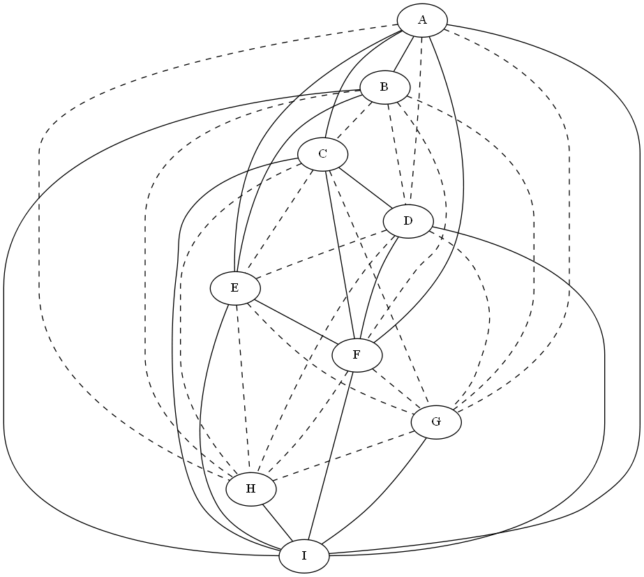
At the beginnig we add vertex $a$ to an empty clan decomposition tree, getting a tree with just one clan. In the next step we add the vertex $b$ to it, having as a result a clan with two maximal strong clans in its coarsest quotient (a complete clan). Both steps are initial cases, they are shown in Figure 22.

When we add $c$ to this clan, we are in the case $1.(b)$ since $a$ is seen from $c$ by the color of the clan but $b$ is not. Thus, the maximal strong clans that are not seen from the color of the clan are moved to another sibling clan, in this case containing $b$ , and $c$ is added to it, in this case we add $c$ to a complete clan with just $b$ in its coarsest quotient (the initial case). All the process is shown in Figure 23.

Now, we have in the root a complete clan and the node $d$ is added to it. We find the new node may not see one of the maximal strong clans in the coarsest quotient of the root, the case $1.(d)$ , center of Figure 24. Thus, the type of the clan is changed to primitive and the maximal strong clans that are seen from $d$ in the same way will conform a new coarsest quotient while those nodes that are not seen from $d$ are split; in this case we do not have any new coarsest quotient and the maximal strong clan conformed by $b$ and $c$ is split, getting as result the decomposition tree shown in the right of Figure 24.

In the next step we add the vertex $e$ to a primitive clan root, left of Figure 25. We find that there is one maximal strong clan $b$ in its coarsest quotient, that sees all the remaining maximal strong clans in the same way than the vertex to be added, the case $2.(a)$ , we can see it in the center of Figure 25. Thus, the new vertex is added to it, the resulting clan decomposition tree is shown in the right of Figure 25.

When we add $f$ to the primitive clan on the root of the current decomposition, left of Figure 26, we find $f$ cannot see one of the maximal strong clans, the clan conform by $b$ and $e$ , as we have a primitive clan we are in case $2.(c)$ , and the elements of the clan are split, right of Figure 26.

In the next step, we add $g$ to the primitive root of this decomposition tree, and we find that $g$ sees all of the maximal strong clans in the coarsest quotient of the root clan in the same way, case $2.(b)$ , center of Figure 27. Thus, this root clan and the new vertex will be in the coarsest quotient of a new complete clan, right of Figure 27.

When we add $h$ to the complete clan in the root of the current decomposition tree, left of Figure 28, we find that $h$ sees in the same way than the color of the clan to all the maximal strong clans in the coarsest quotient of the root clan, the case $1.(a)$ , center of Figure 28. Thus, $h$ is added as another maximal strong clan to the coarsest quotient of the complete clan root, right of Figure 28.

Finally, to add $i$ produces a superior clan, since $i$ sees in the same way all the maximal strong clans of the current root complete clan but different than the color of the clan, the case $1.(c)$ , center of Figure 29. Thus, this root clan and the new vertex will be in the coarsest quotient of a new complete clan, the resulting clan decomposition tree is shown in the right of Figure 29.

Example 7

As an example to show the use of split, assume we add $n$ to the decomposition shown in the left of Figure 30, such that $n$ is connected by solid lines just with $b$ , $c$ , $h$ , $j$ and $l$ .

Following the algorithm we will give the maximal strong clans in the coarsest quotient of the current vertices plus the new vertex $n$ .

Since the coarsest quotient of the root clan is complete those nodes seen in the same way by $n$ will conform a maximal strong clan, in this case we get the clan $\{a,m\}$ . And those nodes that are not visible from $n$ are split, thus we split the clan $\{b,c,d,e\}$ and the clan $\{f,g,h,\{i,j,k,l\}\}$ . When we split the clan $\{b,c,d,e\}$ we have again it is a complete clan, thus following the previous constrains we get $\{b,c\}$ and $\{d,e\}$ as maximal strong clans.

As the clan $\{f,g,h,\{i,j,k,l\}\}$ is a primitive clan, the clans into its coarsest quotient that are seen from $n$ continue being maximal strong clans in the new decomposition, while those clans that are not seen by $n$ are split. In this case we continue having $f$ , $g$ and $h$ as maximal strong clans, and we split the clan $\{i,j,k,l\}$ since it is not possible to determine an edge to it from $n$ . Splitting the clan $\{i,j,k,l\}$ , as it is a complete clan, we get $\{j,l\}$ and $\{i,k\}$ as maximal strong clans.

The resulting decomposition is shown in the right of Figure 30.

6.6 Comparative with Other Algorithms

In this section, we compare our algorithm with a couple of existing algorithms, [12] and [11]: those that we find conceptually closest. We refrain from developing a larger perspective as it would be redundant with an existing, very good survey [8]. We stick to the same terminology of the previous sections (e.g., primitive and complete modules) but warn the reader that the sources may employ different nomenclature.

The algorithm in [12] is applied on undirected graphs and it is not incremental. The algorithm starts by constructing a tree that is modified until reaching the modular decomposition tree, going through three kinds of trees.

In the first kind of tree the internal nodes are labeled primitive or complete by recognizing the $P_{4}$ induced. If the original graph does not induce any $P_{4}$ , the initial graph will have just complete internal nodes.

To get the second kind of tree, only the complete nodes of the previous kind of tree will be analyzed in order to find modules within the complete nodes. To reach the third kind of tree, modules that are not strong are removed.

Example 8

From the left Figure 31 we get $\{f,h,g,abcde\}$ as induced $P_{4}$ , while the graph conformed by $\{a,b,c,d,e\}$ does not induce $P_{4}$ . In this way, the first kind of tree is a tree with two internal nodes, one labeled as primitive and the other one labeled as complete, right of Figure 31.

The next step is to analyze just the complete modules looking for more modules (strong or not), those only could be complete since all primitive ones were obtained in the previous step. We get, among other modules, $\{abc\}$ as complete strong module and in turn $\{a,b,c\}$ are also modules of it, the process to get the second kind of tree is shown in Figure 32.

The last step is to prune the previous tree, removing those modules that are not strong modules. The final decomposition is shown in Figure 33. Thus we illustrate the different modus operandi with respect to our algorithm.

The algorithm in [11] is applied on all 2-structures, not only symmetric; to simplify the comparison, since we work only on symmetric 2-structures, we will avoid those parts referring to linear clans. It is an incremental algorithm that generalizes the elements of the Muller and Spinrad algorithm for decomposition of undirected graphs [13]. Again, despite the fact that this algorithm uses different nomenclature, we will try to explain it using our terminology.

The algorithm works with two trees. One of them keeps the clan decomposition of the graph, each internal node of the tree represents a clan but its internal 2-structure is not shown. The other tree stores node information and information between the nodes by split labels, we will talk a little more about them later.

Example 9

Assume we add the vertex $e$ to the coarsest quotient graph shown in Figure 34. This new vertex does not see some of the clans in it, $F$ and $G$ , and the rest of the elements are seen different than the color of the edges of the coarsest quotient graph, say red (dotted) to $a,b$ and blue (dashed) to $c,d$ , right of Figure 34. Assume $G$ is a primitive clan conform by $g_{1},g_{2},g_{3}$ and $F$ is a complete clan conform by $f_{1},f_{2}$ , whose coarsest quotients are shown in Figure 35; besides, $e$ is connected by different kind of edges with their elements, as shown in Figure 36.

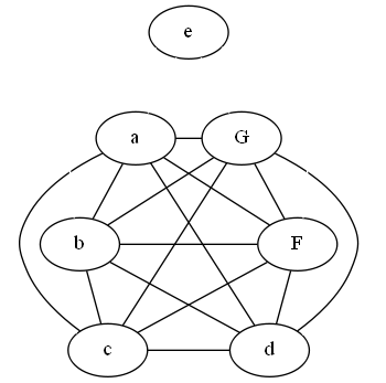
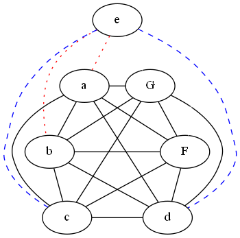
The modular decomposition before to add $e$ is shown in Figure 37. The nodes are filled by white if there is an unambiguous color to connect the node with $e$ , and gray otherwise (“not seen”).

The algorithm ask for the type of the node that is not seen by $e$ . If the node is primitive its children are the same plus the new vertex. Else (the node is complete), its children will be those nodes that are not connected with $e$ by the same kind of edges than the edges of the node.

The other tree stores each visible clan of the previously described tree. If the node is complete its children are grouped according to how they are seen from the new vertex ( $e$ , in this example). The edges are labeled by a split label: $w$ is a split label for the edges $X$ , $Y$ if $(X,w)\neq(Y,w)$ . In this way, this tree works complementing the information about the children of the nodes in the decomposition tree. The final tree decomposition is shown in Figure 38.

The main difference with Algorithm 6 is that, instead of building this tree and doing the labeling process, our algorithm uses the Union-Find structure: each time a new clan is generated, its edges to the other clans (sigleton or not) are added according to their equivalence classes if they exist.

7 Discussion and perspectives

Along this paper, we have shown, first, that the known notion of modular decomposition of a graph can be understood, in a quite natural way from a perspective of data analysis, as a variant of closure space visualization; then, that this process can be applied to transactional datasets via a known logical construction, namely the Gaifman graph; and, also, that both the theoretical connection and the practical applicability of the decomposition process can be generalized to quantitatively enabled variants of Gaifman graphs through a known generalization of modular decompositions, namely the clan decomposition of 2-structures. We have included a number of developments that relate the taxonomy of modules to the corresponding local structure of the closure space, with algorithms to construct the adequate 2-structure to understand which equivalence classes are relevant for the decompositions and which ones are not; and we have described an incremental algorithm, which extends existing ones, that we are currently using in our open-source software tools, https://github.com/MelyPic/Gaifman-graphs_Mod, that we use in order to compute clan decompositions. There is ample room to study improvements to this algorithm and, as mentioned above, the possibilities of using our theoretical results to obtain additional, alternative, hopefully better algorithms.

The avenues for further research are many and wide. First and foremost, additional examples of the practical relevance of this approach are convenient; so far, we can offer some interesting applications in [1] and [2], but we hope to add further, equally convincing case studies down the road.

Along this practical line, we have found many cases where the obtained graphs and decompositions are somewhat too large or complex to provide intuition through diagrams. We have proposed a few simple strategies to encompass complex substructures upon visualization in [1] (our “Others” nodes in the examples, for instance) but a more systematic study of the ways in which visual diagrams can become helpful is necessary; we believe that the answers will come from some notion of interactive data analysis process: hence our insistence that the major decomposition algorithms to be used should be incremental.

Admittedly, our proposals for enhancing Gaifman graphs with quantitative information can be considered simple or even naïve, and must be subject to further testing on practical cases and to comparison with additional alternatives that could be designed in the future. For instance, one may focus on the set of integers arising as multiplicities of each of all the pairs of vertices in our quantitative Gaifman graph, and consider this set of integers as a single-dimensional dataset itself; then, on it, bring to bear existing unsupervised discretization methods in order to split the edges into their corresponding equivalence classes: the options explored here amount to sticking to the “equal length bins” discretization (either on the original data or after a logarithmic scaling), and quite a few additional options exist.

Also, many other tunings can be applied to the Gaifman graph before applying the decomposition procedure. For instance, we have started in [14] the exploration of the case where the equivalence class of the 2-structure edge $(x,y)$ depends on the distance between $x$ and $y$ along a shortest path of the original Gaifman graph. Other similar parameters such as connectivity (number of disjoint paths, that one can relate to Menger’s theorem) could be applied as well.

The multirelational potential is also to be developed. Of course, if we are given a dataset consisting of several tables, it is a simple matter to apply directly our approach as, indeed, Gaifman graphs were defined from the start so as to apply to any relational structure with possibly several tables: a Gaifman edge would join $x$ and $y$ whenever they appear together in some tuple of some table. However, initial explorations in [1] suggest that this naïve application will fall short of providing good results, because a crucial notion in multirelational data, namely foreign keys, is being ignored. How to take foreign keys into account at the time of constructing the Gaifman graph, in a way that provides sensible results in practice, is a question that needs careful exploration, both conceptually and in terms of efficiency (e.g. we could denormalize into a single large table the data through the foreign keys, but this looks like an inefficient implementation even if the process turns out to be practically applicable at all). We believe that a generalization of the “shortest path” variant alluded to above could lead to a working approach.

Further theoretical issues remain open. To mention just two of them: in our scheme according to Figure 2, would there be a way of telling whether a given set of implications will be amenable to the graph reconstruction procedure?, and, regarding the clan taxonomy given the closure space, how to get further information about the internals of each clan in a way similar to the facts we have been able to establish about modules?

Finally, it is well-known that, in data analysis tasks, categorical concepts (such as implications) benefit from a relaxation (such as partial implications or association rules) allowing for exceptions, whether they come from varied inputs or even from material errors in coding or transmission. Likewise, we could relax through allowing exceptions the notions of module and clan. The concept we would end up with seems to us very close to (a recursive form of) the notion of “blockmodeling” employed in social network analysis [4]; this is again a large area where, to start with, a clarification endeavor will be effortful but necessary.

Acknowledgements

We are grateful to Laura Rodríguez-Navas for her help in many ways, to the Hospital de la Santa Creu i Sant Pau for allowing our research group to employ their diagnostic data in our research, and to Ricard Gavaldà who provided the data in such a clean form.

This work was partially supported by European Research Council under the European Union’s Horizon 2020 research and innovation programme, grant agreement ERC-2014-CoG 648276 (AUTAR), by Ministerio de Economia, Industria y Competitividad, project TIN2017-89244-R, and by Conacyt (México). We acknowledge unfunded recognition by AGAUR (Generalitat de Catalunya) as research group 2017SGR-856 (MACDA).

References

[1] Balcázar, J.L., Piceno, M.E., Rodríguez-Navas, L.: Decomposition of quantitative gaifman graphs as a data analysis tool. In: Duivesteijn, W., Siebes, A., Ukkonen, A. (eds.) Advances in Intelligent Data Analysis XVII - 17th International Symposium, IDA 2018, ’s-Hertogenbosch, The Netherlands, October 24-26, 2018, Proceedings. Lecture Notes in Computer Science, vol. 11191, pp. 238–250. Springer (2018), https://doi.org/10.1007/978-3-030-01768-2_20
[2] Balcázar, J.L., Piceno, M.E., Rodríguez-Navas, L.: Hierarchical visualization of co-occurrence patterns on diagnostic data. In: 32nd IEEE International Symposium on Computer-Based Medical Systems, CBMS 2019, Cordoba, Spain, June 5-7, 2019. pp. 168–173 (2019)
[3] Dawson, R.J.M.: The ‘unusual episode’ data revisited. Journal of Statistics Education 3(3) (1995)
[4] Doreian, P., Batagelj, V., Ferligoj, A.: Generalized Blockmodeling. Cambridge University Press (2005)
[5] Dua, D., Graff, C.: UCI machine learning repository (2017), http://archive.ics.uci.edu/ml
[6] Ehrenfeucht, A., Harju, T., Rozenberg, G.: The Theory of 2-Structures - A Framework for Decomposition and Transformation of Graphs. World Scientific (1999), http://www.worldscibooks.com/mathematics/4197.html
[7] Gallai, T.: Transitiv orientierbare graphen. Acta Mathematica Academiae Scientiarum Hungarica 18(1), 25–66 (1967), http://dx.doi.org/10.1007/BF02020961
[8] Habib, M., Paul, C.: A survey of the algorithmic aspects of modular decomposition. Computer Science Review 4(1), 41–59 (2010), https://doi.org/10.1016/j.cosrev.2010.01.001
[9] Libkin, L.: Elements of Finite Model Theory. Texts in Theoretical Computer Science. An EATCS Series, Springer (2004), https://doi.org/10.1007/978-3-662-07003-1
[10] Maffray, F., Preissman, M.: A Translation of Gallai’s Paper: ‘Transitive Orientierbare Graphen’, pp. 25–66
[11] McConnell, R.M.: An O(n²) incremental algorithm for modular decomposition of graphs and 2-structures. Algorithmica 14(3), 229–248 (1995), https://doi.org/10.1007/BF01206330
[12] McConnell, R.M., Spinrad, J.P.: Modular decomposition and transitive orientation. Discrete Mathematics 201(1-3), 189–241 (1999), https://doi.org/10.1016/S0012-365X(98)00319-7
[13] Muller, J.H., Spinrad, J.P.: Incremental modular decomposition. J. ACM 36(1), 1–19 (1989), https://doi.org/10.1145/58562.59300
[14] Piceno, M.E., Rodríguez-Navas, L.: A graphical tool for the interpretation of medical data. In: ACM Celebration of Women in Computing: womENcourage (2019)
[15] Spinrad, J.P.: P ${}_{\mbox{4}}$ -trees and substitution decomposition. Discrete Applied Mathematics 39(3), 263–291 (1992), https://doi.org/10.1016/0166-218X(92)90180-I
[16] Wild, M.: A theory of finite closure spaces based on implications. Advances in Mathematics 108, 118–139 (1994)
[17] Balcázar, J.L., Piceno, M.E., Rodríguez-Navas, L.: Co-occurrence patterns in diagnostic data. Computational Intelligence Journal, 2020, https://doi.org/10.1111/coin.12317.
[18] Rymon, R.: Search through Systematic Set Enumeration. In: Proceedings of the 3rd International Conference on Principles of Knowledge Representation and Reasoning (KR’92), 539–550.
[19] Dechter, R., Pearl, J.: Structure Identification in Relational Data. Artif. Intell. 58 (1992), 237–270.
[20] Khardon, R., Roth, D.: Reasoning with models. Artificial Intelligence 87 (1996), 187–213.
[21] Cormen, T.H., Leiserson,C.E., Rivest, R.L., Stein, C.: Introduction to Algorithms, 3rd Edition, MIT Press. 978-0-262-03384-8, http://mitpress.mit.edu/books/introduction-algorithms.