Distilling Fractons from Layered Subsystem-Symmetry Protected Phases

The parent two-dimensional model is the $d=2$ toric code as introduced in Ref. [12]. The Hilbert space is that of $N=2L^{2}$ qubits where each edge of an $L\times L$ square lattice is associated with a single qubit. The stabilizer set is given by

$b_{p}=\prod_{i\in p}z_{i}$, where $i$ indexes the edge qubits about the plaquette $p$ and $a_{v}=\prod_{i@v}x_{i}$, where $i$ indexes the edge qubits coordinated to the vertex $v$. The toric code hosts two independent topological constraints given by the collection of all stabilizers of a given type. This enforces a global (in the plane) $\mathbb{Z}_{2}$ charge conservation via Theorem 1, whereby the $a_{v}$ terms or “electic sector” must be excited in pairs. Likewise is true for the $b_{p}$ terms or “magnetic sector.” $\mathcal{P}_{\ell}(TC_{2})$ is given by basis members which are characterized as string operators–two for each no-trivial cycle of the 2-torus–given by forming a pair of electric charges or magnetic charges and wrapping them around the system such that the excitations cancel. All operators are shown in Fig. 2 where we find that $\dim P_{\ell}(TC_{2})=4$, $R_{TC_{2}}=L$. Thus the $d=2$ toric code contains LRE.

The target model is referred to as the X-cube model and is the paradigmatic example of a Type-I fracton phase [36]. The Hilbert space is that of $N=3L^{3}$ qubits such that each edge of the cubic lattice is associated with one qubit. The stabilizer set is given by

$a_{v}^{\hat{e}_{j}}=\prod_{i@v_{j}}x_{i}$, where $i$ indexes the qubits coordinated to vertex $v$ and for edges confined to the plane normal to $\hat{e}_{j}$ and $b_{c}=\prod_{i\in c}z_{i}$, where $i$ indexes the qubits about the primitive cube $c$ (see Fig. 3). The properties of the X-cube model are well-known. Elementary excitations of the cube stabilizers are immobile as they cannot hop without generating additional excitations. However, pairs of cubic excitations are free to move in a plane perpendicular to the stacking direction of the two cubes (see Ref. [20] for a thorough discussion of excitation hopping in the X-cube model). This restriction on the mobility is a consequence of the sub-extensive number of constraints among these stabilizers. Such constraints are generated by any set which contains all cubes in a plane perpendicular to a coordinate direction. As a single cube lies at the intersection of three such planar constraints, any syndrome containing that cube must contain at minimum three other excitations, the four of which form a $\mathbb{Z}_{2}$ quadrupole in order to satisfy Theorem 1. As for the vertex stabilizers, they must form a composite excitation of two terms at a given vertex due to the extensive number of trivial constraints. These constraints are generated by any set containing the three stabilizers associated to a given vertex. Furthermore, the collection of all vertex stabilizers whose support is confined to a coordinate plane is also a constraint. So for every composite excitation at a vertex, there is generally the same composite somewhere along the line at the intersection of the two planes containing the two stabilizers forming the composite (there are also three composite configurations which sit on three intersecting lines). It is in this sense that the composite is mobile only along lines and thus deemed “lineons.” Logical operators are the same sting operators as the $d=2$ toric code, but they can only be deformed in coordinate planes. For example, stacked pairs of $Z$-type strings can be deformed in the cubic planes, while $X$-type strings can only be deformed in the coordinate planes. Modding out by these deformations, one finds $\dim\mathcal{P}_{\ell}(XC)=12L-6$ [14] and $R_{XC}=L$ indicating LRE.

Once we stack the layers of the toric code, there are $N=6L^{3}$ qubits and every edge of the cubic lattice represents a two-qubit unit cell. The base model is then given by

Such a stabilizer code is trivial in that $R_{XX}=1$ as given by the fact that $x_{e}^{1}\simeq x_{e}^{2}\in\mathcal{P}_{\ell}(XX)$ and its simultaneous eigenstates are product states within the unit cells.

We now apply Brillouin-Wigner perturbation theory to the X-cube example. As previously stated, the stabilizer nature of the parent and base models allows us to find the terms of the effective Hamiltonian in the Pauli operator basis by considering only products of the parent model which commute with all stabilizers of the base model. The $a_{v}$ terms of the toric code stacks survive at first order as they already commute with the base model stabilizers. These terms alone do not fully lift the extensive base model degeneracy, so we are forced to continue to higher orders. Considering the $b_{p}$ terms of the parent model, it is not until sixth order that some terms survive. In particular, the product of the six plaquette operators about a cube has support in each unit cell of $z_{e}^{1}z_{e}^{2}$ which locally commutes with the base terms $x_{e}^{1}x_{e}^{2}$. It was argued in Ref. [14] that no terms of order less than sixth survive, but we make an argument here as it carries over analogously for the other models. Consider the commutation of base model terms {$(xx)_{e}=x_{e}^{1}x_{e}^{2}\}$ with any product of parent model stabilizers. All such products are represented by the space $\mathcal{A}_{\left(TC_{2}\right)_{\text{stacks}}}=\wp\left(S_{TC_{2}}\right)^{3L}$. Let all products which commute with the base model be represented by a subspace $\mathcal{L}\subseteq\mathcal{A}_{\left(TC_{2}\right)_{\text{stacks}}}$. For $A\in\mathcal{L}$ and using Eq. (10),

So we require that $\mathcal{L}=\left(\psi_{\text{parent}}[\mathcal{G}_{\text{base}}]\right)^{\perp_{\omega}}=\left(\mathrm{Im}\,\psi_{\text{parent}}\phi_{\text{base}}\right)^{\perp_{\omega}}$ which is to say the terms which survive must be orthogonal to the image under $\psi_{\text{parent}}$ of the group of operators generated by the base model terms. That is, we look at the space of parent model excitations generated by base model terms, and any products which overlap an even number of times with those excitations represent the terms which survive the perturbation. The set $\psi_{\text{parent}}\left((xx)_{e}\right)$ is a small p-string wrapping the edge $e$ similar to the one shown in Fig. 1a and from this we see that $\mathrm{Im}\,\psi_{\text{parent}}\phi_{\text{base}}$ is nearly the entire space of p-strings, $\left(\mathcal{D}^{Z}\right)^{\perp_{\omega}}$–the actual imagine does not contain the topologically non-trivial p-strings which wrap the 3-torus. Thus we conclude that $\mathcal{L}=\mathcal{D}^{Z}\oplus\wp\left(S^{X}_{TC_{2}}\right)^{3L}$.⁹⁹ 9 Technically, there are additional members contained in $\left(\mathrm{Im}\,\psi_{\text{parent}}\phi_{\text{base}}\right)^{\perp_{\omega}}$. Because the image only contains closed, trivially-contractible p-strings, its perpendicular complement contains all of $\mathcal{D}^{Z}$, which includes all even numbers of membranes wrapping the cycles, as well as the topologically non-trivial odd numbers of membranes wrapping the cycles, which are not in $\mathcal{D}^{Z}$. However, the image of these wrapping membranes under $\phi_{\text{parent}}$ are also in the image of $\mathcal{D}^{Z}$ because of the planar toric code constraints, so this technical detail does not change the statement. The lowest weight generators for $\mathcal{D}^{Z}$ are the sets $\{b_{p}:p\in c\}$ for every $c$ cube, i.e. the set of six plaquettes which form $c$. Thus no lower order product of plaquettes survive the perturbation. Also note that although we truncate the higher order terms of the effective Hamiltonian, such terms only survive if they land in $\mathcal{D}^{Z}$, so the target model eigenstates are exact and the higher order terms only modify the energy. Finally to see that we completely recover all properties of the X-cube model, we recognize that the infinite perturbation fixes the degrees of freedom associated with the base model such that $x_{e}^{1}\simeq x_{e}^{2}$ and as a result,

which we recognize as the trivial constraint among the vertex terms at $v$.

From the argument for the survival of the sixth order perturbation, we see this process as condensing the p-strings. Moreover, we also recognize the LRE of the X-cube model is inherited from the parent $d=2$ toric code layers. Namely, the string logical operators have an identical form as those from the toric code layers. The only distinction is that due to the coupling, the equivalence classes for these logical string operators are altered. For example, Z-type string operators no longer unambiguously belong to a specific plane, but rather lie at the intersection of two planes. Thus, a single string is ridge along that intersection, but a pair forming a ribbon can be deformed in the plane perpendicular to the stacking direction. This is related to the lack of mobility of vertex bound state excitations. One can also see that topological constraints are inherited from toric code layers. We leave a more detailed discussion of how the anyonic nature of the parent model can be used to understand the fractonic behavior of the X-cube model to Refs. [14, 34]. We do this in part as the parent models for the novel cases below are not anyonic so such details are not helpful for understanding the results below.

As pointed out in Ref. [14, 34], if one were to instead alter the base model to be

the resulting target model becomes the $d=3$ toric code. The $d=3$ toric code Hilbert space is the same as that of the X-cube model and the stabilizer set is given by

where $a^{TC_{3}}_{v}=\prod_{e@v}x_{e}$ or all X-type operators coordinated to $v$ and $b_{p}$ is the same plaquette operators from the $d=2$ toric code. This model is the prototypical stabilizer code example of TO in $d=3$. Excitations of the electric sector, or $\{a^{TC_{3}}_{v}\}$ terms, must be created in pairs as enforced by the constraint consisting of all such operators. Excitations of the magnetic sector, or $\{b_{p}\}$ terms, must form p-strings as enforced by the trivial constraint that the product of the six plaquette operators about any elementary cube is the identity. These excitations must also satisfy a total flux conservation as any p-string must pass through any plane wrapping the 3-torus–which is a constraint–an even number of times. The logical operators are given by Z-type strings that wrap a single direction of the 3-torus, where all such strings wrapping a given cycle are equivalent, and X-type planar operators which wrap any pair of directions of the 3-torus, where all such planar operators wrapping given directions are equivalent. As a consequence $\dim\mathcal{P}_{\ell}(TC_{3})=6$, $R_{TC_{3}}=L$ and this model is LRE.

The perturbation analysis works exactly the same way, but the subspace of the toric code stacks that survives the perturbation is $\wp\left(S^{Z}_{TC_{2}}\right)^{3L}\oplus\overline{\mathcal{D}}^{X}$ where $\overline{\mathcal{D}}^{X}$ is generated by the sets $\{a_{v}^{\hat{e}_{1}},a_{v}^{\hat{e}_{2}},a_{v}^{\hat{e}_{3}}\}$ for every $v$ vertex i.e. the three stabilizers associated to a vertex. Likewise, $z_{e}^{1}\simeq z_{e}^{2}$, which implies for every cube $c$,

One should recognize the connection between the three models $\left(TC_{2}\right)_{\text{stacks}}$, X-cube and $d=3$ toric code. The $XX$ base model is used exactly to condense the p-string excitations of the $d=3$ toric code, whereas the $ZZ$ base model is used to condense the lineon composite excitations of the X-cube model. Likewise, the subspace $\mathcal{D}^{Z}$ which survives the $XX$ base model perturbation is exactly the space which forms the trivial kernel of $\phi_{TC_{3}}$ i.e these operators are “removed” by becoming the identity, whereas the space $\overline{\mathcal{D}}^{X}$ which survives the $ZZ$ base model perturbation is exactly the space which forms the trivial kernel of $\phi_{XC}$. We also recognize that $\dim\mathcal{P}_{\ell}\left(\left(TC_{2}\right)_{\text{stacks}}\right)=\dim\mathcal{P}_{\ell}(XC)+\dim\mathcal{P}_{\ell}(TC_{3})$. Thus, it would seem that all the LRE of the toric code stacks is “conserved” between these two models. All these facts are not coincidental. We argue below that these are all a consequence of the statement,

where equivalence and direct sum are defined in the category of $\mathbb{F}_{2}$-linear gauge structures. The existence of such a co-target model–which the $d=3$ toric code is in this case– is exactly our definition of a condensation process and is made precise in Section 4.3. Any case where no such co-target exists is then defined as a distillation process.

The parent model is composed of a CSS variant of the cluster model as introduced in Ref. [26]. The Hilbert space is that of $N=2L^{2}$ qubits with two qubits associated with each vertex. The stabilizer set is given by

where $c^{X}_{v},c^{Z}_{v}$ are defined in Fig. 4.¹⁰¹⁰ 10 To see this equivalent to the cluster model, One can follow Ref. [37] where the usual cluster model has been coarse-grained from one qubit per vertex to two qubits per vertex. Then by applying a Hadamard gate to every second qubit in a vertex unit cell, one finds our version. To understand this model, consider applying $z^{1}_{v}\text{id}_{v}^{2}$ for some vertex $v$. This excites only $c^{X}_{v}$, and likewise, $\text{id}_{v}^{1}x_{v}^{2}$ only excites $c_{v}^{Z}$. Using general combinations of these operators, this implies that we can achieve any syndrome/excitation configuration. This further implies the constraint space is trivial by Theorem 1, and because the number of stabilizers is equal to the number of qubits, it must be that $d_{\ell}=0$ and $R_{Cl}=0$. Thus, the cluster model contains no LRE, and it would seem there is nothing of interest. However, one can assert that there are special members of $\mathcal{G}_{Cl}$ which are referred to as subsystem symmetries (SS). Consider the product of all $c_{v}^{X}$ along any rigid line in a coordinate direction, and likewise for $c_{v}^{Z}$. The resulting operators are

where $(e_{1},e_{2})\in\mathbb{Z}_{L}^{2}$ indexes a vertex of the graph, as shown in Fig. 4. As argued in Ref. [26], these stabilizer group members gain significance if we limit the operators which act on our system to a subspace of the Pauli space $\mathcal{R}\subseteq\mathcal{P}$ containing all operators which commute with the subsystem symmetries. As the subsystem symmetries are in $\mathcal{G}_{Cl}$, $\mathcal{R}$ must contain all of $\mathcal{G}_{Cl}$, in which case it is reasonable to only consider $\mathcal{R}/\mathcal{G}_{Cl}\simeq\mathcal{R}^{\prime}$, where $\mathcal{R}^{\prime}$ is the set of all operators generated by $x^{1}_{v}\text{id}_{v}^{2}$ and $\text{id}_{v}^{1}z_{v}^{2}$ for all $v$. Note this excludes operators generated by $z^{1}_{v}\text{id}_{v}^{2}$ and $\text{id}_{v}^{1}x_{v}^{2}$, the exact operators we used to generate an arbitrary syndrome. We are now free to ignore any part of the stabilizers which commute with all $\mathcal{R}^{\prime}$ since they no long affect the syndromes as generated by the function $\psi$ after we limit ourselves to $\mathcal{R}^{\prime}$. The subspace that commutes with all of $\mathcal{R}^{\prime}$ is just $\mathcal{R}^{\prime}$ as it is a maximal, mutually commuting set. As a result, all subsystem symmetries in Eqs.(26) effectively become constraints and as a result imply effective conservation laws via Theorem 1. Looking back to Fig. 4, one can see that removing operators from $\mathcal{R}^{\prime}$ makes the cluster model into two copies of the Ising plaquette model. The Ising plaquette model is a classical model with one qubit (or classical spin) per vertex of the square lattice and stabilizers given by

Action by $x_{v}$ creates a $\mathbb{Z}_{2}$ quadrupole and in general, excitations must satisfy $\mathbb{Z}_{2}$ conservation laws along all rigid $d=1$ subsystems in the coordinate directions, exactly the conservation laws implied by Eqs. (26) when all operators from $\mathcal{R}^{\prime}$ are removed. This model is also the paradigm example of fractons in two dimensions [39] (though not FTO strictly speaking). This process of restricting to subspaces of operators is exactly the idea behind a gauge substructure as introduced in Section 4.2.

We refer to the target model as the cluster-cube model and to the best of our knowledge, this is its first introduction in the literature. The Hilbert space is that of $N=2L^{3}$ qubits arranged on the cubic lattice such that there are two qubits associated to each vertex. The stabilizer set is given by

where $cc_{v}^{X},cc_{v}^{Z}$ are defined in Fig. 5. We focus on the $cc_{v}^{X}$ terms, where all the same properties are present for the $cc_{v}^{Z}$ terms if one applies the clear duality between these two types of stabilizers. If we apply the operator $z_{v}^{1}\text{id}_{v}^{2}$ at some vertex $v$, one excites four cube stabilizers whose centers form an “upward-facing” right-angled tetrahedron (henceforth just referred to as a UF tetrahedron). Likewise, applying the operator $z_{v}^{1}z_{v}^{2}$ at $v$ generates a tetrahedral pattern which is symmetric to the first by inversion in the $[111]$ direction or a “downward-facing” (DF) tetrahedron. As a result, one can generate the syndrome such that all eight cubes about $v$ are excited. Applying the same operator to an adjacent vertex is equivalent to pulling apart two bound states of four excitations. One can continue in this fashion until the four-excitation bound states are annihilated and so the resulting string operator must commute with all $\mathcal{G}_{CC}$. It should be clear that this string operator is not a member of $\mathcal{G}_{CC}$ and is therefore in $\mathcal{P}_{\ell}(CC)$. To characterize such string operators as logical operators, we need to determine their equivalence classes. Consider taking the product of cube stabilizers along a ridge line in a coordinate direction–similar to that of the subsystem symmetries for the cluster model. If this one dimensional subsystem is, for example, along the $[100]$ direction, then the resulting operator is equivalent to the product of two of our logical operators which both lie in the plane perpendicular to the $[011]$ direction. This implies all logical string operators in the $[011]$ plane are equivalent in $\mathcal{P}_{\ell}(CC)$, and likewise for stings in the $[101]$ and $[110]$ planes. The “dual” logical operators which anti-commute with the string logical operators are diagonal string operators which are discussed in detail in Section 4.5.2. Furthermore, as we can take pairs of string operators in the $[011],[101]$ and $[110]$ planes, move them apart via the $d=1$ subsystem product of stabilizers and eventual cancel them out so as to remove all support, this implies that any set of cubes forming a $[110],[101]$ or $[011]$ plane is a topological constraints and implies a planar $\mathbb{Z}_{2}$ charge conservation similar to the X-cube model. Also like the X-cube model, $[110],[101]$ and $[011]$ constraints intersect at a single cube stabilizer, implying fractonic behavior similar to X-cube. As the four-cube bound state is mobile and are found at the end of string operators, this model fits the definition of a Type I fracton model.

One might be tempted to classify this model as equivalent to X-cube, but string operators are not the only logical operators. If we start from either one of the tetrahedral configurations, we can apply the same operator to adjacent vertices, thereby un-exciting three of the original tetrahedron of cubes and exciting four cubes of a larger tetrahedron as shown if Fig. 6. This process can be continued such that we excite the corners of larger and larger tetrahedra and if the system size is such that $L=2^{a}$ for some integer $a$, then these corners annihilate with one another after $a$ generations. The resulting operator which commutes with all of $\mathcal{G}_{CC}$ can be described as a three-dimensional, right-angled version of the Sierpinski fractal. We argue below that this cannot be equivalent to any combination of string operators, nor is it a product of stabilizers. However, not all translated versions of such fractal logical operators are distinct in $\mathcal{P}_{\ell}(CC)$. Consider that a cube stabilizer can be thought of as an UF and DF tetrahedron which are “glued” together. The UF tetrahedron is formed from only $x_{v}^{1}x_{v}^{2}$ operators and the DF tetrahedron is formed from only $\text{id}_{v}^{1}x_{v}^{2}$ operators. In the same manner as our process for forming the fractal logical operators, we can remove all support of a given type, say $x_{v}^{1}x_{v}^{2}$, out to the corners of an ever larger UF tetrahedron and at the $a^{th}$ generation, those four points overlap and all such support is removed. We consider this operator to be a fractal SS operator and is equivalent to the product of four fractal logical operators. To see this, consider our fractal product of stabilizers at some generation less than $a$. Now imagine we remove the four $x_{v}^{1}x_{v}^{2}$ corners and consider the syndrome the resulting operator creates. Naturally, this operator generates the same syndrome as the four $x_{v}^{1}x_{v}^{2}$ corners we removed and can be described as four elementary DF tetrahedral configurations (among the the $cc_{v}^{Z}$ operators) centered on vertices of an UF tetrahedron which then annihilate with each other at the $a^{th}$ generation. This implies our fractal SS must be equivalent to four of the UF fractal logical operators arranged in a DF tetrahedron configuration. Furthermore as this is a stabilizer group element, these four fractal logical are equivalent to the identity in $\mathcal{P}_{\ell}(CC)$. Such fractal SS operators also allow us to understand the additional fractal constraints which are implied by the existence of the fractal logical operators. If we represent a fractal logical operator by a single base-point, then a UF fractal SS operator is equivalent to four logical operators whose base-points form an elementary DF tetrahedron. Again, we can combine SS fractals in an analogous DF fractal such that the four logical operator base-points are moved along the corners of a fractal and eventually annihilate with one another. The resulting product of SS fractals, which are themselves products of stabilizers must be equivalent to the identity, and thus this collection of stabilizers is a constraint which enforces the fractal hopping of the excitations.

At this time, we make no attempt at counting the number of independent logical operators, i.e. calculate the GSD for this model, as the exact number is not important for the remaining discussion and may be a complicated function of $L$. We only note that $\log_{2}$GSD scales as $\sim L$ which is a common feature of fractonic models. The string operators imply that $R_{CC}=L$ which implies this model contains LRE.

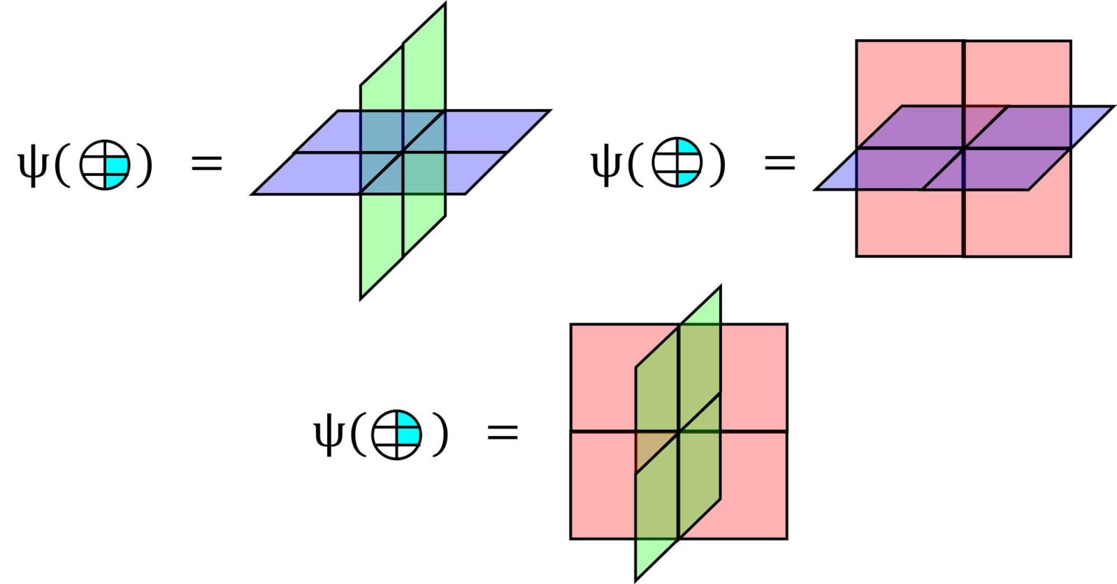
Once we combine the three stacks of cluster models, the resulting Hilbert space can be characterized as $N=6L^{3}$ qubit where each vertex represents a six qubit unit cell. It is best to further break this up into two unit cells of three qubits. For ease of notation, we then define the following three-qubit operators,

Note that $(xxx)^{1}(xxx)^{2}(xxx)^{3}=\text{id}$, $(zzz)^{1}(zzz)^{2}(zzz)^{3}=\text{id}$, and the commutation relations can be summarized as $\lambda\left((xxx)^{i},(zzz)^{j}\right)=1$ for $i\neq j$ and $i,j=1,2,3$, $\lambda\left((xxx)^{0},(zzz)^{0}\right)=1$ and all other pairs commute.

For reasons we discuss below, there are multiple possible base models, but we focus on one as it is the most “local”. The stabilizers are given by

Just as with the X-cube example, this perturbation model is trivial with $R_{c\text{-}\triangle}=1$ and simple product eigenstates in the local vertex Hilbert spaces. The name $c\text{-}\triangle$ is explained below.

To understand the structure of the stacking, we organize the layers so the $x_{v}^{1}x_{v}^{2}$ base points of $c_{v}^{X}$ in each layer meets at the “origin point” of the elementary cube. This maintains a three-fold rotation symmetry about the $[111]$ axis. As a consequence, the $z_{v}^{1}z_{v}^{2}$ base points of $c_{v}^{Z}$ in each layer meet at the origin antipode of the elementary cube (see Fig. 8).

Just as with the X-cube example, the perturbation analysis of the cluster cube requires us to determine which product of parent model stabilizers commute with the base model. For $\mathcal{A}_{Cl_{\text{stacks}}}=\wp\left(S_{cl}\right)^{3L}$, let $\mathcal{D}^{X}$ be the same subspace generated by the set of six X-type stabilizers which form a cube and likewise for $\mathcal{D}^{Z}$ using Z-type stabilizers. X-type p-strings are then members of $\left(\mathcal{D}^{X}\right)^{\perp_{\omega}}$ and Z-type p-strings are members of $\left(\mathcal{D}^{Z}\right)^{\perp_{\omega}}$. Following the same procedure as X-cube, we consider the space $\mathrm{Im}\,\psi_{\text{parent}}\phi_{\text{base}}$ which is partially generated by the set $\psi_{\text{parent}}\left(\text{id}_{v}\otimes(zzz)_{v}^{i}\right)$. From the definitions in Eqs. (29), one finds that $\psi_{\text{parent}}\left(\text{id}_{v}\otimes(zzz)_{v}^{i}\right)$ contains two small X-type p-strings about the two edges coordinated to $v$ and extending in the $\hat{e}_{i}$ direction as depicted in Fig. 7. Likewise, $\psi_{\text{parent}}\left((xxx)^{i}_{v}\otimes\text{id}_{v}\right)$ contains similar Z-type p-strings. Note these pairs of p-strings are rigid along this line, i.e. no operators of the base model can “turn” one p-string relative to the other in any plane. This already suggests that the set of terms which survive the perturbation, specifically those from $\left(\mathrm{Im}\,\psi_{\text{parent}}\phi_{\text{base}}\right)^{\perp_{\omega}}$ includes the subspace $\mathcal{D}^{X}\oplus\mathcal{D}^{Z}$. Again, other products can be found in $\left(\mathrm{Im}\,\psi_{\text{parent}}\phi_{\text{base}}\right)^{\perp_{\omega}}$, even more so than in the X-cube example, and furthermore, we lack any constraints. In particular, $\left(\mathrm{Im}\,\psi_{\text{parent}}\phi_{\text{base}}\right)^{\perp_{\omega}}$ contains all sets of configurations forming a rigid $d=1$ line in any plane –exactly those forming the subsystem symmetries of the cluster model layers, and so these products survive and are not trivial. Such operators only appear at $L^{th}$ order in the perturbation and are exponentially suppressed in $L$, however, we show in Section 4.5.2 that the appearance of such operators “breaks” the symmetry of the ground space and fixes which target model ground state we obtain.

So again, the lowest order to survive the perturbation is sixth order and this contributes terms to the effective Hamiltonian given by the product of stabilizers which form a cube and only products of these cubes survive for higher orders, except for the subsystem symmetries which appear at $L^{th}$ order. This alone does not guarantee that the effective Hamiltonian corresponds to the cluster-cube model. If we take the product of cluster model operators which form the cube as in Fig. 8, we find that in terms of the operators defined in Eqs. (29), the resulting product is the cluster cube operators written in terms of the $(xxx)^{0}$ or$(zzz)^{0}$ operators times ($+$ in $\mathcal{P}$) a triangle operator, $t_{c}^{X}$ or $t_{c}^{Z}$, which is written in terms of the $(xxx)^{i}$ or $(zzz)^{i}$ operators for $i=1,2,3$. Even more specific, they are written in terms of the base model operators which implies $t_{c}^{X},t_{c}^{Z}\in\mathcal{G}_{\text{base}}$. So as a result of the infinite perturbation which fixes the degrees of freedom for the base model, $t_{c}^{X},t_{c}^{Z}\simeq\text{id}_{\mathcal{H}}$. This implies our cube operators become that of the cluster cube on effective qubit degrees of freedom defined by the local Pauli algebra generated by $(xxx)^{0}$ and $(zzz)^{0}$.

The parent model for this example is a $d=2$ SSPT model which we refer to as the quasi-cluster model. To the best of our knowledge, this is the first introduction of this model in the literature. The Hilbert space for the quasi-cluster model is given by $N=2L^{2}$ with the stabilizer set given by

which are defined in Fig. 9.¹¹¹¹ 11 One can equivalently define this model by reflection of the stabilizers about the main diagonal. Either version can be used for this example. We apply the same analysis as with the cluster model, whereby we consider acting with $z_{v}^{1}z_{v}^{2}$ for any $v$. This excites only $qc_{v}^{X}$. Likewise, acting with $x_{v}^{1}x_{v}^{2}$ excites only $qc_{v}^{Z}$. By the same logic as used for the cluster model, this implies $d_{\ell}=0$, $R_{qCl}=0$ and thus this model is SRE. Furthermore, we consider the $d=1$ subsystem symmetries given by

We again follow the same logic by considering restricting to $\mathcal{R}^{\prime}\simeq\mathcal{R}/\mathcal{G}_{qCl}$, where $\mathcal{R}$ is all Pauli operators which commute with the subsystem symmetries. $\mathcal{R}^{\prime}$ can be described as all operators generated by $z_{v}^{1}\text{id}_{v}^{2}$ and $\text{id}_{v}^{1}x_{v}^{2}$ which forms a maximal, mutually commuting subset of $\mathcal{P}$ and just as before, modding out by $\mathcal{R}^{\prime}$ implies our subsystem symmetries are effectively constraints and our stabilizer code becomes two independent stacks of classical Ising chains in the $\hat{e}_{2}$ direction.

There is another subsystem symmetry which, although not as clean, essentially has the same properties. For the $qc_{v}^{X}$ terms, one recognizes that if we ignore the first qubit at every vertex, these terms have the form of the Newman-Moore model [16]. This is a classical model of $L^{2}$ qubits (or classical spins) arranged on the triangular lattice with one qubit per vertex and the stabilizer set given by

In our case, we have just skewed the lattice so that the elementary triangles form right angles. For an $L=2^{a}$ sized lattice, the product of triangle stabilizers in the form of an $a^{th}$-generation Sierpinski fractal only has support on the three corners of the fractal which now overlap on a single point. This almost suffices to form a constraint and even though it does not do so exactly, it does enforce a local version of Theorem 1. This results in the usual fractonic properties of the Newman-Moore model which requires that excitation must be created locally in threes and can only be moved along the ends of a fractal. In the case of the quasi-cluster model, we can form the same fractal to obtain the subsystem symmetries

where $\text{Sierpinski}_{v}$, is the usual Sierpinski fractal, and $\widetilde{\text{Sierpinski}}_{v}$ is the alternative Sierpinski fractal as shown on the right side of Fig. 9. The primed versions are given by reflecting about the $\hat{e}_{1}=-\hat{e}_{2}$ line. Because the base point of $s_{v}^{X},s_{v}^{Z}$ is not a part of the fractal, we cannot apply the same logic as the other subsystem symmetries. Still, we can restrict to the set of Pauli operators generated by $x_{v}^{1}\text{id}_{v}^{2}$ and $\text{id}_{v}^{1}z_{v}^{2}$, in which case our stabilizers become two independent copies of the Newman-Moore model and the fractal subsystem maps to the product of Newman-Moore stabilizers and the local fractal charge conservation is enforced.

The target model is Haah’s cubic code–or just Haah’s code–which is the paradigmatic example of Type-II fractons. The Hilbert space is given by $N=2L^{3}$ qubit arranged on the cubic lattice such that each vertex represents a two qubit unit cell. The stabilizers are given by

where $g_{c}^{X}$ and $g_{c}^{Z}$ are defined in Fig. 10. We primarily study this model by considering the $g_{v}^{X}$ operators, but analogous statements hold for the $g_{v}^{Z}$ operators by the obvious symmetry between these operators. Applying $x_{v}^{1}\text{id}_{v}^{2}$ generates the same UF tetrahedron excitation pattern as Fig. 6, so excitation again move on the ends of a fractal operator and for $L=2^{a}$ we find fractal logical operators. Applying $\text{id}_{v}^{1}x_{v}^{2}$ instead generates a regular tetrahedron pattern and a similar process results in a different fractal logical operator with a regular tetrahedron geometry. By design, Haah’s code contains no string logical operators. To the best of our knowledge, the constraints of Haah’s code are not discussed in the literature except for a maximum of 7 found in [25] which represent all constraints which are periodic in the $[111]$ direction. This clearly cannot be sufficient to characterize all constraint or else excitations would be free to move in the $[111]$ direction, which is not the case. However like the cluster-cube example, we can find a sub-extensive number of constraints that enforce this fractonic mobility. Looking at Fig. 10, we see that just as with the cluster-cube, we can view $g_{v}^{X}$ as the product of two tetrahedron, an UF right-angle tetrahedron formed using $\text{id}_{v}^{1}x_{v}^{2}$ operators and a regular tetrahedron using $x_{v}^{1}\text{id}_{v}^{2}$ operators. So for $L=2^{a}$, we can again multiply the $g_{v}^{X}$ operators in a fractal pattern, thereby removing all $x_{v}^{1}\text{id}_{v}^{2}$ support, or with a different fractal, all $\text{id}_{v}^{1}x_{v}^{2}$ support. By the same arguments as the cluster-cube model, we again find the fractal subsystem symmetry composed of four logical operators, and just as before, these SS can be multiplied in a fractal way such that the resulting product maps to the identity, thus constituting a constraint. The number of independent constraints of this form must scale with the system size. It is known that for $L=2^{a}$ [11, 10], $d_{\ell}=4L-2$ which must also be the dimension of the constraint space. As there are no string operators for this code, the fractal logical operators determine the code distance. Counting the number of single qubit Pauli’s needed to form these fractals, one finds $R_{\text{Haah}}\leq 4^{(a-1)}=\frac{1}{4}L^{2}$. Though these fractal logical operators are deformable and this bound may not be tight, it should be clear that $R_{\text{Haah}}\gtrsim L$, so this model contains LRE [11].

Just as with the cluster-cube example, we form the three stacks of the quasi-cluster model which yields a Hilbert space of $N=6L^{3}$ qubits arranged on the cubic lattice such that there are six qubits associated with each vertex. We also divide each of these unit cells into two three qubit unit cells. The stabilizer set of the base model is

where $h_{c}^{X},t_{c}^{X},h_{c}^{Z},t_{c}^{Z}$ are defined in Fig. 11a. We refer to $h_{c}^{X},h_{c}^{Z}$ as hexagon operators, but it may be more appropriate to visualize them as two triangle operators similar to $t_{c}^{X},t_{c}^{Z}$ stacked in the $[111]$ direction. We recognize that these are rather complicated operators and arguably more so that the target model. This is a consequence of the construction of Section 4.4 which only guarantees the perturbation model is no “less local” than the target model. However, we are allowed a great deal of freedom, even removing the condition that it is a stabilizer Hamiltonian in order to simply the base model. We discuss this in Section 4.5.4.

This model contains four layer constraints for every $[111]$ layer, one for each stabilizer type. It is equivalent to stacks of a variant of the $d=2$ toric code on the triangular lattice which is depicted in Fig. 11b. This implies that $R_{c\text{-}\text{hex}}=L$ and the model contains LRE.

To understand the structure of the stacking, we organize the layers so the $x_{v}^{1}x_{v}^{2}$ right-angle base-points of $qc_{v}^{X}$ in each layer meets at the origin point of the elementary cube and the arrows in Fig. 9 meet tip-to-tail where stabilizers between different layers meet (see Fig. 12). This maintains a three-fold rotation symmetry about the $[111]$ axis. As a consequence, the $z_{v}^{1}z_{v}^{2}$ right-angle base-points of $c_{v}^{Z}$ in each layer meet at the origin antipode of the elementary cube and the direction of the associated arrows is reversed.

Much of the analysis from the cluster-cube example carries over. In particular, we take the product of the six quasi-cluster plaquettes which form a cube and rewrite this operator by separating the $(xxx)^{0},(zzz)^{0}$ degrees of freedom from the $(xxx)^{j},(zzz)^{j}$ degrees of freedom as shown in Fig. 12. From this, one can see this product of quasi-cluster operators is equivalent to the product of the $g_{c}^{X},g_{c}^{Z}$ operators using the $(xxx)^{0},(zzz)^{0}$ degrees of freedom times ($+$ in $\mathcal{P}$) the $h_{c}^{X},h_{c}^{Z}$ operators using the $(xxx)^{j},(zzz)^{j}$ degrees of freedom. Since the base model operators are completely written in the $(xxx)^{j},(zzz)^{j}$ degrees of freedom, then this sixth order perturbation term survives if and only if $h_{c}^{X},h_{c}^{Z}$ commutes with the entire base model, which by construction, it does. Furthermore, the strong perturbation is such that $h_{c}^{X}\simeq h_{c}^{Z}\simeq\text{id}_{\mathcal{H}}$, implying these sixth order terms are equivalent to the terms of Haah’s code. All that’s left is to argue no lower order terms survive the perturbation. As before we consider the subspace of all terms which survive the perturbation $\left(\mathrm{Im}\,\psi_{\text{parent}}\phi_{\text{base}}\right)^{\perp_{\omega}}$. Members of $\mathrm{Im}\,\psi_{\text{parent}}\phi_{\text{base}}$ are generated by the p-string configurations shown in Fig. 13. Due to the complexity of these p-strings, it is not immediately clear what other configurations, besides members of $\mathcal{D}^{X}\oplus\mathcal{D}^{Z}$, are orthogonal to these p-strings, but it is clear that they must be greater than sixth-order and scale with the size of the system. This is discussed in greater detail in Section 4.5.3.

References

- [1] Charles. Bennett, Herbert. Bernstein, Sandu Popescu and Benjamin Schumacher “Concentrating partial entanglement by local operations” In Phys. Rev. A 53 American Physical Society, 1996, pp. 2046–2052 DOI: 10.1103/PhysRevA.53.2046
- [2] Bernhard. Bodmann et al. “Frame theory for binary vector spaces”, 2009 eprint:arXiv:0906.3467
- [3] Sergey Bravyi, Bernhard Leemhuis and Barbara. Terhal “Topological order in an exactly solvable 3D spin model” In Ann. Phys. 326.4, 2011, pp. 839–866 DOI: 10.1016/j.aop.2010.11.002
- [4] Claudio Chamon “Quantum Glassiness in Strongly Correlated Clean Systems: An Example of Topological Overprotection” In Phys. Rev. Lett. 94 American Physical Society, 2005, pp. 040402 DOI: 10.1103/PhysRevLett.94.040402
- [5] Trithep Devakul “Classifying local fractal subsystem symmetry-protected topological phases” In Phys. Rev. B 99 American Physical Society, 2019, pp. 235131 DOI: 10.1103/PhysRevB.99.235131
- [6] Trithep Devakul, Dominic. Williamson and Yizhi You “Classification of subsystem symmetry-protected topological phases” In Phys. Rev. B 98 American Physical Society, 2018, pp. 235121 DOI: 10.1103/PhysRevB.98.235121
- [7] Trithep Devakul, Yizhi You, F.. Burnell and S.. Sondhi “Fractal Symmetric Phases of Matter” In SciPost Phys. 6 SciPost, 2019, pp. 7 DOI: 10.21468/SciPostPhys.6.1.007
- [8] D. Gottesman “Stabilizer codes and quantum error correction”, 1997
- [9] Jeongwan Haah “Commuting Pauli Hamiltonians as maps between free modules” In Communications in Mathematical Physics 324.2 Springer, 2013, pp. 351–399
- [10] Jeongwan Haah “Lattice quantum codes and exotic topological phases of matter”, 2013 eprint:arXiv:1305.6973
- [11] Jeongwan Haah “Local stabilizer codes in three dimensions without string logical operators” In Phys. Rev. A 83 American Physical Society, 2011, pp. 042330 DOI: 10.1103/PhysRevA.83.042330
- [12] A Kitaev “Fault-tolerant quantum computation by anyons” In Annals of Physics 303.1 Elsevier, 2003, pp. 2–30
- [13] Aleksander Kubica and Beni Yoshida “Ungauging quantum error-correcting codes”, 2018 eprint:arXiv:1805.01836
- [14] H. Ma, E. Lake, X. Chen and M. Hermele “Fracton topological order via coupled layers” In ArXiv e-prints, 2017 arXiv:1701.00747 [cond-mat.str-el]
- [15] Rahul. Nandkishore and Michael Hermele “Fractons”, 2018 eprint:arXiv:1803.11196
- [16] M… Newman and Cristopher Moore “Glassy dynamics and aging in an exactly solvable spin model” In Phys. Rev. E 60 American Physical Society, 1999, pp. 5068–5072 DOI: 10.1103/PhysRevE.60.5068
- [17] Z. Nussinov and G. Ortiz “Sufficient symmetry conditions for Topological Quantum Order” In Proceedings of the National Academy of Science 106, 2009, pp. 16944–16949 DOI: 10.1073/pnas.0803726105
- [18] Zohar Nussinov and Gerardo Ortiz “A symmetry principle for topological quantum order” In Annals of Physics 324.5, 2009, pp. 977–1057 DOI: https://doi.org/10.1016/j.aop.2008.11.002
- [19] Shriya Pai and Michael Hermele “Fracton fusion and statistics”, 2019 eprint:arXiv:1903.11625
- [20] Abhinav Prem, Jeongwan Haah and Rahul Nandkishore “Glassy quantum dynamics in translation invariant fracton models” In Phys. Rev. B 95 American Physical Society, 2017, pp. 155133 DOI: 10.1103/PhysRevB.95.155133
- [21] Michael Pretko “Generalized electromagnetism of subdimensional particles: A spin liquid story” In Phys. Rev. B 96 American Physical Society, 2017, pp. 035119 DOI: 10.1103/PhysRevB.96.035119
- [22] Michael Pretko “Subdimensional particle structure of higher rank spin liquids” In Phys. Rev. B 95 American Physical Society, 2017, pp. 115139 DOI: 10.1103/PhysRevB.95.115139
- [23] Robert Raussendorf, Daniel. Browne and Hans. Briegel “Measurement-based quantum computation on cluster states” In Phys. Rev. A 68 American Physical Society, 2003, pp. 022312 DOI: 10.1103/PhysRevA.68.022312
- [24] J.J. Sakurai and J. Napolitano “Modern Quantum Mechanics” Addison-Wesley, 2011 URL: https://books.google.com/books?id=N4I-AQAACAAJ
- [25] Albert. Schmitz “Gauge structures: From stabilizer codes to continuum models” In Annals of Physics 410, 2019, pp. 167927 DOI: https://doi.org/10.1016/j.aop.2019.167927
- [26] Albert. Schmitz, Sheng-Jie Huang and Abhinav Prem “Entanglement spectra of stabilizer codes: A window into gapped quantum phases of matter” In Phys. Rev. B 99 American Physical Society, 2019, pp. 205109 DOI: 10.1103/PhysRevB.99.205109
- [27] Wilbur Shirley, Kevin Slagle and Xie Chen “Fractional excitations in foliated fracton phases”, 2018 eprint:arXiv:1806.08625
- [28] Wilbur Shirley, Kevin Slagle and Xie Chen “Universal entanglement signatures of foliated fracton phases” In SciPost Phys. 6 SciPost, 2019, pp. 15 DOI: 10.21468/SciPostPhys.6.1.015
- [29] Kevin Slagle and Yong Kim “X-cube model on generic lattices: Fracton phases and geometric order” In Phys. Rev. B 97 American Physical Society, 2018, pp. 165106 DOI: 10.1103/PhysRevB.97.165106
- [30] David. Stephen et al. “Subsystem symmetries, quantum cellular automata, and computational phases of quantum matter” In ArXiv e-prints, 2018 arXiv:1806.08780 [quant-ph]
- [31] Barbara. Terhal “Quantum error correction for quantum memories” In Rev. Mod. Phys. 87 American Physical Society, 2015, pp. 307–346 DOI: 10.1103/RevModPhys.87.307
- [32] M. Tinkham “Group Theory and Quantum Mechanics”, Dover Books on Chemistry and Earth Sciences Dover Publications, 2003 URL: https://books.google.com/books?id=r4GIU2wJCAEC
- [33] G. Vidal “Entanglement Renormalization” In Phys. Rev. Lett. 99 American Physical Society, 2007, pp. 220405 DOI: 10.1103/PhysRevLett.99.220405
- [34] S. Vijay “Isotropic Layer Construction and Phase Diagram for Fracton Topological Phases” In ArXiv e-prints, 2017 arXiv:1701.00762 [cond-mat.str-el]
- [35] Sagar Vijay, Jeongwan Haah and Liang Fu “A new kind of topological quantum order: A dimensional hierarchy of quasiparticles built from stationary excitations” In Phys. Rev. B 92 American Physical Society, 2015, pp. 235136 DOI: 10.1103/PhysRevB.92.235136
- [36] Sagar Vijay, Jeongwan Haah and Liang Fu “Fracton topological order, generalized lattice gauge theory, and duality” In Phys. Rev. B 94 American Physical Society, 2016, pp. 235157 DOI: 10.1103/PhysRevB.94.235157
- [37] D.. Williamson, A. Dua and M. Cheng “Spurious topological entanglement entropy from subsystem symmetries” In ArXiv e-prints, 2018 arXiv:1808.05221 [quant-ph]
- [38] Dominic. Williamson, Zhen Bi and Meng Cheng “Fractonic matter in symmetry-enriched gauge theory” In Phys. Rev. B 100 American Physical Society, 2019, pp. 125150 DOI: 10.1103/PhysRevB.100.125150
- [39] Han Yan “Hyperbolic fracton model, subsystem symmetry, and holography” In Phys. Rev. B 99 American Physical Society, 2019, pp. 155126 DOI: 10.1103/PhysRevB.99.155126
- [40] Beni Yoshida “Exotic topological order in fractal spin liquids” In Phys. Rev. B 88 American Physical Society, 2013, pp. 125122 DOI: 10.1103/PhysRevB.88.125122
- [41] Yizhi You, Trithep Devakul, F.. Burnell and S.. Sondhi “Subsystem symmetry protected topological order” In Phys. Rev. B 98 American Physical Society, 2018, pp. 035112 DOI: 10.1103/PhysRevB.98.035112