On the Non-monotonicity of entropy for a class of real quadratic rational maps

Khashayar Filom and Kevin M. Pilgrim Address: Khashayar Filom, Department of Mathematics, Northwestern University; Email address: khashayarfilom2014@u.northwestern.edu Address: Kevin M. Pilgrim, Department of Mathematics, Indiana University; Email address: pilgrim@indiana.edu

Date: June 2020

Abstract.

We prove that the entropy function on the moduli space of real quadratic rational maps is not monotonic by exhibiting a continuum of disconnected level sets. This entropy behavior is in stark contrast with the case of polynomial maps, and establishes a conjecture on the failure of monotonicity for bimodal real quadratic rational maps of shape $(+-+)$ which was posed in [Fil19] based on experimental evidence.

1. Introduction

The variation of entropy in a family of dynamical systems is a natural indication of the change of dynamics through the family that could shed light on the nature of bifurcations. There is a vast literature on the entropy behavior of interval maps. In particular, Milnor’s conjecture on the monotonicity of entropy claims that the entropy level sets – the isentropes – are connected within families of polynomial interval maps whose critical points are all real [vS14]. The monotonicity of entropy for polynomial interval maps was first established for quadratic polynomials [DH85, MT88, Dou95]. In case of the logistic family

(1.1)

\left\{x\mapsto\mu x(1-x):[0,1]\to[0,1]\right\}_{0\leq\mu\leq 4},

this monotonicity result states that the entropy is non-decreasing with respect to the parameter $\mu$ . Next, the monotonicity conjecture was settled in the case of cubic polynomials in [DGMT95, MT00]. In the general setting of boundary-anchored polynomial interval maps of a fixed degree and shape and with real non-degenerate critical points, the monotonicity of entropy has been established in [BvS15], and also in [Koz19] with a different method.

In this paper we are concerned with rational maps rather than polynomials. After some effort one can still set up an entropy function on an appropriate moduli space of real rational maps [Fil18]. When the degree is two, the space $\mathcal{M}_{2}(\mathbb{R})$ of Möbius conjugacy classes of real quadratic rational maps may be naturally identified with the real plane $\mathbb{R}^{2}$ [Mil93, §10]. Assigning to each conjugacy class $\langle f\rangle$ the topological entropy of the restriction to the real circle $\hat{\mathbb{R}}:=\mathbb{R}\cup\{\infty\}$ of a representative $f$ defines a continuous real entropy function

(1.2)

h_{\mathbb{R}}:\langle f\rangle\mapsto h_{\rm{top}}\left(f\restriction_{\hat{\mathbb{R}}}\hat{\mathbb{R}}\rightarrow\hat{\mathbb{R}}\right)\in\left[0,\log(2)\right]

on an appropriate open subset of $\mathcal{M}_{2}(\mathbb{R})$ . The numerically generated entropy contour plots in [Fil19] suggested that the isentropes are connected in certain dynamically defined regions of the moduli space whereas are disconnected in another region of dynamical interest; namely, the region of $(+-+)$ -bimodal maps. The former was partially resolved in that paper ([Fil19, Theorem 1.2]) while the non-monotonicity part was stated merely as a conjecture ([Fil19, Conjecture 1.4]). The main goal of this paper is to establish this anticipated failure of monotonicity; see Theorem 1.1 below. We prove the non-monotonicity of the real entropy function $h_{\mathbb{R}}$ by studying certain $(+-+)$ -bimodal real quadratic rational maps. Our arguments easily imply the non-monotonicity for the restriction of $h_{\mathbb{R}}$ to the $(+-+)$ -bimodal region as well.

Theorem 1.1.

There exists a real number $h^{\prime}\in\left(0,\log(2)\right)$ with the property that for every entropy value $h\in\left(h^{\prime},\log(2)\right)$ the level set $h_{\mathbb{R}}=h$ is disconnected.

In fact, we can take $h^{\prime}$ to be the logarithm of the largest real root of $t^{3}-2t^{2}+1=0$ :

(1.3)

h^{\prime}=\log\left(\frac{1+\sqrt{5}}{2}\right).

The main idea of the proof is to construct certain unbounded hyperbolic components – denoted by $\mathcal{H}_{p/q}$ – of $\mathcal{M}_{2}(\mathbb{R})$ , and then to use the elementary fact that the entropy remains constant throughout any real hyperbolic component. After a brief review based on [Ree90, Mil93] of the background material on the moduli space of quadratic rational maps and its hyperbolic components in §2, we construct such unbounded hyperbolic components in §3. The main ingredient of the construction is to exhibit certain post-critically finite (PCF for short) real hyperbolic rational maps $f_{p/q}$ with a specified dynamics on $\hat{\mathbb{R}}$ which lie at the center of the aforementioned hyperbolic components $\mathcal{H}_{p/q}$ . The construction, a special case of [PT98], is topological and utilizes Thurston’s characterization of rational maps [DH93]. Next, we proceed in §3 with an analysis of the limit points of $\mathcal{H}_{p/q}$ in a compactification of $\mathcal{M}_{2}(\mathbb{R})\cong\mathbb{R}^{2}$ to a closed disk. The analysis of the degeneration of hyperbolic components $\mathcal{H}_{p/q}$ is reminiscent of ideas developed in [Pil94, Tan02], and also relies on [Pet93]. The proof of the main theorem finally appears in §4, and utilizes the properties of components $\mathcal{H}_{p/q}$ discussed in the previous section, an entropy monotonicity result of Levin, Shen, and van Strien [LSv19, Theorem 7.2], and planar topology arguments.

Acknowledgments. K.F. is grateful to Laura DeMarco for helpful conversations and suggestions, to Yan Gao for introducing him to paper [LSv19], and to the department of mathematics at Indiana University Bloomington for its hospitality during visits in September 2018 and May 2019. K.M.P. was supported by Indiana University Bloomington and Simons Foundation collaboration grant No. 245269.

2. Background on the Moduli Space and Hyperbolic Components of Quadratic Rational Maps

The goal of this section is to present a brief account of the moduli space of (real or complex) quadratic rational maps including the dynamical coordinate system that identifies the moduli space with a plane, the corresponding compactifications, the seven different topological types of a real quadratic rational map, the experimental evidence on which Theorem 1.1 is based; and finally, the hyperbolic components of quadratic rational maps which are vital to the proof of the theorem.

The complex moduli space $\mathcal{M}_{2}(\mathbb{C})$ of quadratic rational maps is defined as the space

{\rm{Rat}}_{2}(\mathbb{C})\big/{\rm{PSL}}_{2}(\mathbb{C})=\left\{f\mid f\text{ a rational map of degree two}\right\}\big/f\sim\alpha\circ f\circ\alpha^{-1}

of Möbius conjugacy classes of rational maps $f:\hat{\mathbb{C}}\rightarrow\hat{\mathbb{C}}$ of degree two. The conjugacy class of $f$ is denoted by $\langle f\rangle\in\mathcal{M}_{2}(\mathbb{C})$ . This space could famously be identified with the plane $\mathbb{C}^{2}$ [Mil93]. To elaborate, recall that such a map $f$ has three fixed points (counted with multiplicity) whose multipliers – denoted by $\mu_{1}$ , $\mu_{2}$ and $\mu_{3}$ – are related by the holomorphic fixed point formula (see [Mil06, §12])

(2.1)

\frac{1}{1-\mu_{1}}+\frac{1}{1-\mu_{2}}+\frac{1}{1-\mu_{3}}=1.

This amounts to a constraint on the symmetric functions

(2.2)

\sigma_{1}=\mu_{1}+\mu_{2}+\mu_{3},\quad\sigma_{2}=\mu_{1}\mu_{2}+\mu_{2}\mu_{3}+\mu_{3}\mu_{1},\quad\sigma_{3}=\mu_{1}\mu_{2}\mu_{3},

of these multipliers given by $\sigma_{3}=\sigma_{1}-2$ . The conjugacy-invariant functions $\sigma_{1}$ and $\sigma_{2}$ then identify $\mathcal{M}_{2}(\mathbb{C})$ with $\mathbb{C}^{2}$ .

As we are concerned with the dynamics on the real line union infinity $\hat{\mathbb{R}}$ , only the conjugacy classes of real quadratic rational maps $f\in{\rm{Rat}}_{2}(\mathbb{R})$ under the action of ${\rm{PGL}}_{2}(\mathbb{R})$ are relevant to our discussion. The functions $\sigma_{i}$ ’s may be described in terms of coefficients of the rational map $f$ . For instance, in the mixed normal form

(2.3)

\frac{1}{\mu}\left(z+\frac{1}{z}\right)+a

where the critical points and a fixed point are specified, $\sigma_{1}$ and $\sigma_{2}$ are given by the formulas below adapted from [Mil93, Appendix C]:

(2.4)

\begin{cases}\sigma_{1}=\mu(1-a^{2})-2+\frac{4}{\mu}\\ \sigma_{2}=\left(\mu+\frac{1}{\mu}\right)\sigma_{1}-\left(\mu^{2}+\frac{2}{\mu}\right)\end{cases}.

Therefore, $\sigma_{1}$ and $\sigma_{2}$ are real once $f$ lies in ${\rm{Rat}}_{2}(\mathbb{R})$ . Conversely, any point of $\mathcal{M}_{2}(\mathbb{C})\cong\mathbb{C}^{2}$ with real coordinates can be represented by a real map: If the multiplier $\mu$ in (2.4) is real (that is, a real root of the real cubic $z^{3}-\sigma_{1}z^{2}+\sigma_{2}z-\sigma_{3}=0$ ), the real-ness of $\sigma_{1}$ and $\sigma_{2}$ requires $a$ to be either real, or purely imaginary of the form ${\rm{i}}b$ with $b$ real. In the latter situation, after a conjugation with $z\mapsto\frac{z}{{\rm{i}}}$ we arrive at a real map of the form

(2.5)

\frac{1}{\mu}\left(z-\frac{1}{z}\right)+b.

We deduce that the space

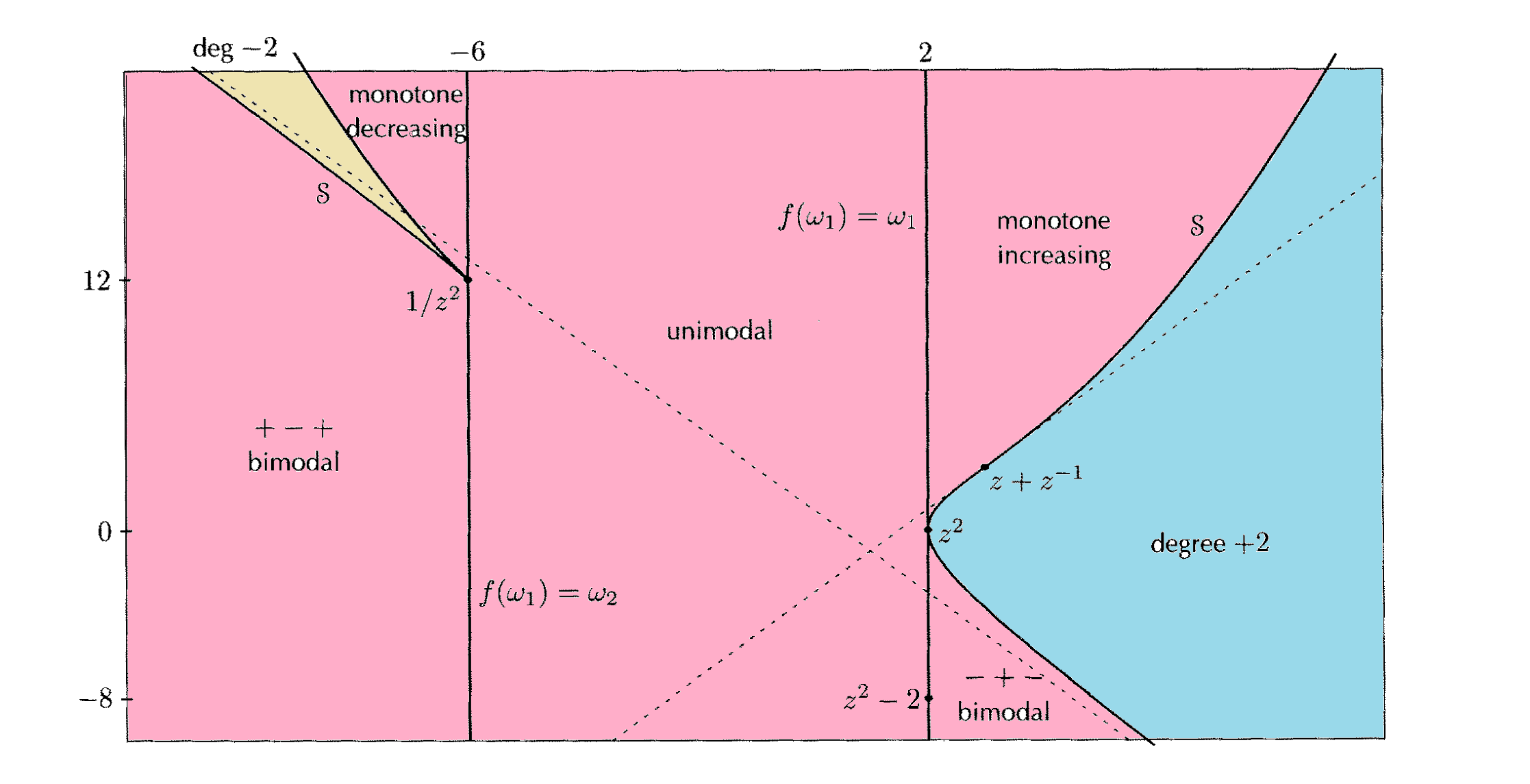
\mathcal{M}_{2}(\mathbb{R})={\rm{Rat}}_{2}(\mathbb{R})\big/{\rm{PSL}}_{2}(\mathbb{R})

of the conjugacy classes of real maps could be identified with the underlying real plane $\mathbb{R}^{2}$ [Mil93, §10]. Figure 1 adapted from Milnor’s paper illustrates the moduli space $\mathcal{M}_{2}(\mathbb{R})$ in the $(\sigma_{1},\sigma_{2})$ coordinate system. The paper then proceeds with a careful examination of $\mathcal{M}_{2}(\mathbb{R})$ based on the real dynamics which we shall review below:

•

The restriction $f\restriction_{\hat{\mathbb{R}}}:\hat{\mathbb{R}}\rightarrow\hat{\mathbb{R}}$ is either a two-sheeted covering map or is not surjective in which case both critical points of $f$ are real, and the topological degree of $f\restriction_{\hat{\mathbb{R}}}:\hat{\mathbb{R}}\rightarrow\hat{\mathbb{R}}$ is zero [Fil19, Proposition 2.4].
•

In the case of topological degree zero, the image of $f$ is a compact interval $f(\hat{\mathbb{R}})$ . From the dynamical standpoint, one can solely concentrate on the interval map

$f\restriction_{f(\hat{\mathbb{R}})}:f(\hat{\mathbb{R}})\rightarrow f(\hat{\mathbb{R}}).$

Conditioning on its modality (how many critical points lie in $f(\hat{\mathbb{R}})$ ) and shape (whether it starts with an increase or a decrease), one obtains the smaller monotone increasing, monotone decreasing, unimodal, $(+-+)$ -bimodal and $(-+-)$ -bimodal regions within the non-covering part of $\mathcal{M}_{2}(\mathbb{R})$ . These along with degree $\pm 2$ regions comprise the seven regions partitioning the moduli space $\mathcal{M}_{2}(\mathbb{R})$ in Figure 1.

•

The degree $\pm 2$ regions are separated from the union of the other five regions – which we call the component of degree zero maps – via the real part of the symmetry locus

\mathcal{S}(\mathbb{R})=\left\{f\in{\rm{Rat}}_{2}(\mathbb{R})\mid f\text{ has a non-trivial M\"{o}bius automorphism}\right\};

see Figure 2. The symmetry locus is thoroughly studied in [Mil93, §5]. The real entropy (1.2) is multi-valued at the points of $\mathcal{S}(\mathbb{R})$ as they represent maps of the form $\frac{1}{\mu}(z\pm\frac{1}{z})$ which are conjugate only via non-real Möbius transformations and thus, restrict to dynamically distinct self-maps of $\hat{\mathbb{R}}$ : The map $x\mapsto\frac{1}{\mu}\left(x-\frac{1}{x}\right)$ is covering and hence of entropy $\log(2)$ whereas $x\mapsto\frac{1}{\mu}\left(x+\frac{1}{x}\right)$ is of entropy zero [Fil19, Example 2.2].

Refer to caption — Figure 1. The real moduli space $\mathcal{M}_{2}(\mathbb{R})$ as illustrated in [Mil93, Figure 15]. The post-critical lines $\sigma_{1}=-6,2$ ( $\omega_{1},\omega_{2}$ denote the critical points of $f$ here), the dotted lines ${\rm{Per}}_{1}(\pm 1)$ , the real symmetry locus $\mathcal{S}(\mathbb{R})$ and the partition into seven regions according to the various types of the dynamics induced on $\hat{\mathbb{R}}$ are shown. The component of degree zero maps in $\mathcal{M}_{2}(\mathbb{R})-\mathcal{S}(\mathbb{R})$ is the union of monotonic, unimodal and bimodal regions that overlap only along the lines $\sigma_{1}=-6,2$ .

After excluding the symmetry locus, the real entropy (1.2) gives rise to a single-valued function

(2.6)

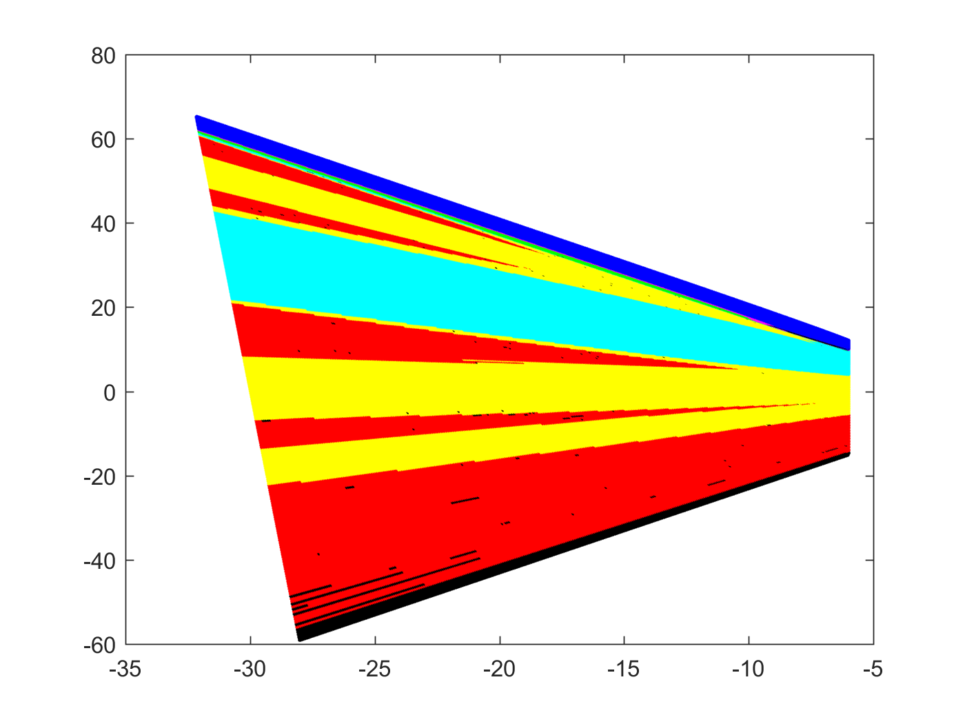
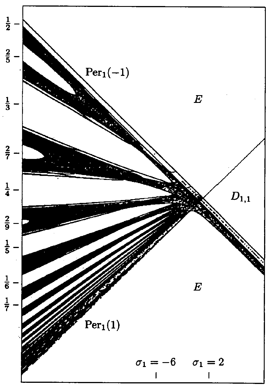
\begin{cases}h_{\mathbb{R}}:\mathcal{M}_{2}(\mathbb{R})-\mathcal{S}(\mathbb{R})\rightarrow\left[0,\log(2)\right]\\ h_{\mathbb{R}}(\langle f\rangle):=h_{\rm{top}}\left(f\restriction_{\hat{\mathbb{R}}}:\hat{\mathbb{R}}\rightarrow\hat{\mathbb{R}}\right)=h_{\rm{top}}\left(f\restriction_{f(\hat{\mathbb{R}})}:f(\hat{\mathbb{R}})\rightarrow f(\hat{\mathbb{R}})\right)\end{cases}

which is continuous [Mis95]. The domain of definition has three connected components; see Figure 2. In our treatment of the monotonicity problem, only unimodal and bimodal regions matter as $h_{\mathbb{R}}\equiv\log(2)$ over the degree $\pm 2$ components of the domain while $h_{\mathbb{R}}\equiv 0$ over the monotonic regions of the component of degree zero maps. A rather lengthy analysis of the dynamics in the degree zero case reduces everything to the study of certain families of unimodal and bimodal interval maps for which entropy plots could be generated numerically [Fil19, §§4,5]. It is observed that the entropy level sets appear disconnected for $(+-+)$ -bimodal maps (see Figure 3) while they appear connected throughout the adjacent unimodal and $(-+-)$ -bimodal regions. Proving the former is the main goal of this paper, and the latter is partially established in [Fil19, Theorem 1.2]: The restriction of $h_{\mathbb{R}}$ to the part of Figure 1 which lies below the dotted line

(2.7)

{\rm{Per}}_{1}(1):\sigma_{2}=2\sigma_{1}-3

is monotonic. This line is dynamically significant as it is where one of the fixed points becomes parabolic. Maps of degree zero below it possess three real fixed points with one of them attracting. In particular, the entropy is monotonic throughout the entirety of the $(-+-)$ -bimodal region where the dynamics is restricted due to the presence of an attracting fixed point [Mil93, Lemma 10.1]. On the contrary, the fixed points of the $(+-+)$ -maps which we shall construct in the next section are repelling (and also not all real). Therefore, their dynamics is essentially non-polynomial in the sense of [Mil00].

Remark 2.1.

The disconnectedness of the domain of the entropy function (2.6) suggests that one should phrase the question of monotonicity of $h_{\mathbb{R}}$ for level sets in just one component of the domain. But as mentioned above, $h_{\mathbb{R}}\equiv\log(2)$ for maps of degree $\pm 2$ ; and in Theorem 1.1 we are dealing with entropy values in $\left(0,\log(2)\right)$ . Therefore, we focus on isentropes in the component of degree zero maps hereafter.

Before proceeding with a discussion of hyperbolic components in $\mathcal{M}_{2}(\mathbb{R})$ , we point out that symmetric functions (2.2) of the multipliers could also be used to describe certain compactifications of moduli spaces $\mathcal{M}_{2}(\mathbb{R})$ and $\mathcal{M}_{2}(\mathbb{C})$ . We shall need such compactifications in §4. One could compactify $\mathcal{M}_{2}(\mathbb{C})\cong\mathbb{C}^{2}$ to the complex projective plane $\widehat{\mathcal{M}_{2}(\mathbb{C})}\cong\mathbb{CP}^{2}$ in which case the added points correspond to degenerate limits of families of quadratic rational maps [Mil93, §4]. To be more precise, notice that if one of the multipliers in (2.1), say $\mu_{3}$ , tends to infinity, the product $\mu_{1}\mu_{2}$ of the other two tends to $1$ ; and

(2.8)

\frac{\sigma_{2}}{\sigma_{1}}=\frac{\mu_{1}\mu_{2}+\mu_{2}\mu_{3}+\mu_{3}\mu_{1}}{\mu_{1}+\mu_{2}+\mu_{3}}=\frac{\frac{\mu_{1}\mu_{2}}{\mu_{3}}+\mu_{2}+\mu_{1}}{\frac{\mu_{1}}{\mu_{3}}+\frac{\mu_{2}}{\mu_{3}}+1}\to\mu_{1}+\frac{1}{\mu_{1}}.

In case that one of $\mu_{1}$ or $\mu_{2}$ becomes unbounded too, the other one must tend to $0$ because of (2.1); so the limit in (2.8) would be infinity. We conclude that the points at infinity could be thought of as unordered triples $\left\{\mu,\mu^{-1},\infty\right\}$ where $\mu$ belongs to $\hat{\mathbb{C}}:=\mathbb{C}\cup\{\infty\}$ . The sum $\mu+\mu^{-1}\in\hat{\mathbb{C}}$ now serves as a coordinate parameterizing the subset of points at infinity as a copy of the Riemann sphere. The real moduli space $\mathcal{M}_{2}(\mathbb{R})$ is the real $(\sigma_{1},\sigma_{2})$ -plane where the slope appeared in (2.8) is real. Hence the closure $\widehat{\mathcal{M}_{2}(\mathbb{R})}$ of $\mathcal{M}_{2}(\mathbb{R})\cong\mathbb{R}^{2}$ in $\widehat{\mathcal{M}_{2}(\mathbb{C})}\cong\mathbb{CP}^{2}$ could be identified with the real projective plane $\mathbb{RP}^{2}$ since it is obtained by adding a copy of $\mathbb{RP}^{1}$ (the space of lines in $\mathbb{R}^{2}$ ) to $\mathbb{R}^{2}$ . Nevertheless, we shall describe another compactification homeomorphic to a disk which is more convenient to work with. For $\sigma_{1}$ and $\sigma_{2}$ real, the corresponding limit points would be triples $\left\{\mu,\mu^{-1},\infty\right\}$ in which $\mu$ belongs to either $\hat{\mathbb{R}}$ , or to the unit circle due to the fact that $\mu+\mu^{-1}$ is required to be real in view of (2.8). Replacing $\mu$ with $\mu^{-1}$ if necessary, one may take $\mu$ to be in the interval $[-1,1]$ , or on the half-arc $\left\{e^{{\rm{i}}\theta}\mid\theta\in[0,\pi]\right\}$ respectively. The union of these two is a circle which serves as the boundary of a new compactification $\overline{\mathcal{M}_{2}(\mathbb{R})}$ . This is a closed disk fibered above $\widehat{\mathcal{M}_{2}(\mathbb{R})}\cong\mathbb{RP}^{2}$ . We record this discussion for the future usage.

Proposition 2.2.

Adding the boundary circle

(2.9)

{\rm{S}}^{1}_{\infty}:=[-1,1]\bigcup\left\{e^{{\rm{i}}\theta}\mid\theta\in[0,\pi]\right\}

to $\mathcal{M}_{2}(\mathbb{R})\cong\mathbb{R}^{2}$ results in a compactification $\overline{\mathcal{M}_{2}(\mathbb{R})}$ of the real moduli space $\mathcal{M}_{2}(\mathbb{R})$ homeomorphic to a closed disk with the following topology: The limit in $\overline{\mathcal{M}_{2}(\mathbb{R})}$ of the conjugacy classes of a sequence $\left\{g_{n}\right\}_{n=1}^{\infty}$ of real quadratic rational maps that degenerate as $n\uparrow\infty$ is a point $\mu\in{\rm{S}}^{1}_{\infty}$ provided that there is a sequence $\left\{p_{n}\right\}_{n=1}^{\infty}\subset\mathbb{CP}^{1}$ of fixed points with $g^{\prime}_{n}(p_{n})\to\mu$ .

Remark 2.3.

The two constituent parts of the circle at infinity (2.9) correspond to different types of real dynamics. Given a sequence $\left\{g_{n}\right\}_{n=1}^{\infty}$ of real quadratic rational maps, when the limit multiplier is $\mu\in(-1,1)$ , it means that the other limit multiplier $\mu^{-1}$ is real as well, and hence for $n$ large enough the map $g_{n}$ has three real fixed points. As $n\uparrow\infty$ , one of the corresponding multipliers blows up and the other two tend to the real numbers $\mu$ and $\mu^{-1}$ . In contrast, when the maps $g_{n}$ have a conjugate pair of fixed points and a real fixed point whose multiplier tends to infinity, the limit point on ${\rm{S}}^{1}_{\infty}$ would be a point $e^{{\rm{i}}\theta}$ from the unit circle. The latter is the case for $(+-+)$ -bimodal maps which we study in this paper.

We finish with a brief treatment of the hyperbolic components of the moduli space of quadratic rational maps. Recall that a rational map is called hyperbolic if each of its critical orbits converges to an attracting cycle; equivalent characterizations could be found in [Mil06, Theorem 19.1]. The paper [Ree90] divides the hyperbolic components of the critically marked moduli space ([Mil93, §6])

(2.10)

\begin{split}&\mathcal{M}_{2}^{\rm{cm}}(\mathbb{C}):={\rm{Rat}}_{2}^{\rm{cm}}(\mathbb{C})\big/{\rm{PSL}}_{2}(\mathbb{C})\\ &=\left\{(f,c_{0},c_{1})\mid f\text{ a rational map of degree two with critical points }c_{0},c_{1}\right\}\Bigg/\begin{matrix}(f,c_{0},c_{1})\sim\\ \left(\alpha\circ f\circ\alpha^{-1},\alpha(c_{0}),\alpha(c_{1})\right)\end{matrix}\end{split}

into four classes and investigates their topological types. The corresponding topological types in the unmarked space $\mathcal{M}_{2}(\mathbb{C})$ can then be deduced [Mil93, §7]. Here, we summarize the four different classes of hyperbolic quadratic maps.

•

Type B: Bitransitive. Both critical orbits converge to the same attracting periodic orbit but critical points are in immediate basins of different points of this orbit.
•

Type C: Capture. Only one critical point lies in the immediate basin of an attracting periodic point and the other critical orbit eventually lands there.
•

Type D: Disjoint Attractors. The critical orbits converge to distinct periodic orbits.
•

Type E: Escape. Both critical orbits converge to the same attracting fixed point. This is the only situation where the Julia set of a hyperbolic quadratic rational maps is disconnected (indeed, a Cantor set) [Mil93, Lemma 8.2].

There are infinitely many hyperbolic components of types B, C or D. As components in $\mathcal{M}_{2}(\mathbb{C})$ , they are topological four cells. The same remains true in the marked space $\mathcal{M}_{2}^{\rm{cm}}(\mathbb{C})$ with the exception of the component of type B that contains $z\mapsto\frac{1}{z^{2}}$ ; the component that we disregard in the proof of Theorem 1.1; cf. Remark 3.5. On the contrary, there is precisely one hyperbolic component of type E which is homeomorphic to $\mathbb{D}\times(\mathbb{C}-\overline{\mathbb{D}})$ [Mil93, Lemma 8.5] ( $\mathbb{D}$ the open unit disk). The escape component is furthermore different in the sense that it is the only hyperbolic component lacking a so-called center – every other component contains a unique PCF map to which we refer as its center.

The real hyperbolic components obtained from non-empty intersections of complex hyperbolic components with $\mathcal{M}_{2}(\mathbb{R})$ pertain to our treatment of the real entropy for the following reasons:

•

the real entropy of a hyperbolic map is the logarithm of an algebraic number and hence $h_{\mathbb{R}}$ is constant over any real hyperbolic component due to its continuity;
•

the dynamics on $\hat{\mathbb{R}}$ of the post-critically finite map at the center admits a Markov partition which allows us to calculate the entropy over the component.

Convention 2.4.

The intersection of any complex hyperbolic component in $\mathcal{M}_{2}(\mathbb{C})$ with $\mathcal{M}_{2}(\mathbb{R})$ , if non-vacuous, is connected and contains the center except for the escape component which does not have a center and its intersection with $\mathcal{M}_{2}(\mathbb{R})$ has two connected components on which $h_{\mathbb{R}}$ is either identically zero or identically $\log(2)$ [Fil19, §3]. We shall refer to these real escape components as the $h_{\mathbb{R}}\equiv 0$ escape component and the $h_{\mathbb{R}}\equiv\log(2)$ escape component. Given a complex hyperbolic component $\mathcal{H}\subset\mathcal{M}_{2}(\mathbb{C})$ different from the escape component, by abuse of notation, we show the (connected) real hyperbolic component $\mathcal{H}\cap\mathcal{M}_{2}(\mathbb{R})$ by $\mathcal{H}$ as well. The hyperbolic component in $\mathcal{M}^{\rm{cm}}_{2}(\mathbb{C})$ to which $\mathcal{H}$ lifts is shown by $\mathcal{H}^{\times}$ .

In the next section, we construct a class of bitransitive real hyperbolic components with known entropy values via introducing their centers.

3. Constructing Unbounded Hyperbolic Components $\mathcal{H}_{p/q}$

The current section is the main technical part of the paper. We first construct a family of hyperbolic PCF quadratic rational maps in Proposition 3.2 with real coefficients and a comprehensible dynamics on $\hat{\mathbb{R}}$ . We then proceed with an analysis of the real hyperbolic components they determine in $\mathcal{M}_{2}(\mathbb{R})$ and the closure of these components in the compactification $\overline{\mathcal{M}_{2}(\mathbb{R})}$ : In Propositions 3.8 and 3.9 we present a family of curves in the aforementioned components and study their limit points as the maps degenerate.

Convention 3.1.

In this section $q$ is an integer larger than one, $p$ belonging to the set $\{1,\dots,q-1\}$ is an integer coprime to $q$ , and $p^{\prime}$ denotes the multiplicative inverse of $p$ modulo $q$ ; i.e. the unique element of that set satisfying $pp^{\prime}\equiv 1\pmod{q}$ . The indices are always considered modulo $q$ and hence are treated as elements of $\mathbb{Z}/q\mathbb{Z}$ . The critical points are denoted by $c_{0}$ and $c_{1}$ .

The following proposition is the key construction of this paper.

Proposition 3.2.

Let $q\geq 2$ be an integer and $p/q\in\mathbb{Q}/\mathbb{Z}$ a fraction in lowest terms. There exists a unique critically finite quadratic rational map $f:=f^{\times}_{p/q}$ with the following properties:

a.

(marked critical points) the two critical points $c_{0},c_{1}$ are labeled;
b.

(the real condition) $f$ has real coefficients;
c.

(normalization) $c_{0}=0$ , $f({\rm{i}})={\rm{i}},f(-{\rm{i}})=-{\rm{i}}$ ;
d.

(bitransitive) the critical points $c_{0},c_{1}$ lie in a cycle of period $q$ , so the post-critical set ${\rm{P}}_{f}$ of $f$ is given by $\left\{f^{\circ j}(c_{0})\right\}_{j=0}^{q-1}$ ;
e.

(rotation number) ${\rm{P}}_{f}$ is a subset of circle $\hat{\mathbb{R}}=\mathbb{R}\cup\{\infty\}$ equipped with its usual orientation; alternatively, we may write its elements as $\{x_{0},x_{1},\ldots,x_{q-1}\}$ where

(3.1) $0=c_{0}=x_{0}<x_{1}<x_{2}<\ldots<x_{q-1}<0;$

then we have

$f(x_{j})=x_{j+p}$

for all $j\in\mathbb{Z}/q\mathbb{Z}$ , so that the restriction $f\restriction_{{\rm{P}}_{f}}:{\rm{P}}_{f}\rightarrow{\rm{P}}_{f}$ forms a cycle with rotation number $p/q$ ;
f.

(adjacent critical points) $c_{1}=x_{1}$ , which in conjunction with the previous property implies $f^{\circ p^{\prime}}(c_{0})=c_{1}$ ;

(Markov partition for real dynamics) for $j\in\mathbb{Z}/q\mathbb{Z}$ define intervals in $\hat{\mathbb{R}}$ by

I_{j}:=[x_{j},x_{j+1}].

Then

(3.2)

\begin{split}&f(I_{0})=I_{0}\cup I_{1}\cup\ldots\cup\underbrace{I_{p}}_{\text{omitted}}\cup\ldots\cup I_{q-1}\\ &f(I_{j})=I_{j+p},\,j=1,\dots,q-1.\end{split}

Furthermore, $f\restriction_{I_{0}}$ reverses orientation while $f\restriction_{I_{j}},\,j\neq 0$ preserves orientation;

h.

(entropy) the topological entropy $h_{q}$ of $f\restriction_{\hat{\mathbb{R}}}$ is the logarithm of the largest positive real root $r_{q}$ of

(3.3) $t^{q-1}-t^{q-2}-\ldots-t^{2}-t-1=\frac{t^{q}-2t^{q-1}+1}{t-1};$
i.

(basins and their boundaries) for $j\in\mathbb{Z}/q\mathbb{Z}$ let $\Omega_{j}$ be the immediate super-attracting basin containing $x_{j}$ ; then each $\Omega_{j}$ is a Jordan domain, and $\partial\Omega_{j}\supset\{\pm{\rm{i}}\}$ ;
j.
(distinguished repelling $q$ -cycle) $\partial\Omega_{0}\cap\hat{\mathbb{R}}$ consists of two points, with a unique positive real element $\zeta_{0}>0$ , which is periodic of exact period $q$ ; we denote the remaining elements in this cycle by $\zeta_{j}\in\partial\Omega_{j},\,j=1,\ldots,q-1$ , so that $f(\zeta_{j})=\zeta_{j+p}$ . They are deployed on the circle $\hat{\mathbb{R}}$ as follows (cf. Figure 4):
1. I.
  
  $x_{0}=0<\zeta_{0}<\zeta_{1}<x_{1}$ ,
2. II.
  
  for $j=1,\ldots,p^{\prime}$ : $\zeta_{jp}<x_{jp}$ ,
3. III.
  
  for $j=1,\ldots,q-p^{\prime}$ : $x_{1+jp}<\zeta_{1+jp}$ ;
k.

(normalized basin coordinates) there exist unique Riemann maps (extended to the boundaries) $\phi_{j}:(\overline{\mathbb{D}},0,1)\rightarrow(\overline{\Omega_{j}},x_{j},\zeta_{j}),j\in\mathbb{Z}/q\mathbb{Z}$ . The first-return map of the immediate basin $\Omega_{0}$ to itself, in these coordinates, is

$\phi_{j}^{-1}\circ f^{\circ q}\circ\phi_{j}:(\mathbb{D},0,1)\rightarrow(\mathbb{D},0,1);$

and is given by $\omega\mapsto\omega^{4}$ .

Proof.

The proof has three different facets:

•

constructing $f_{p/q}$ as a two-sheeted topological branched cover $S^{2}\rightarrow S^{2}$ , proving that it is realized as a rational map via invoking Thurston’s characterization of rational maps [DH93], and establishing the uniqueness – statements a through f;
•

investigating the real dynamics and the corresponding Markov partition – statements g and h;
•

analyzing the Fatou components – statements i through k.

Existence. We construct a critically finite topological branched self-cover of the sphere, denoted by $G$ , with similar properties, but with the post-critical set in the unit circle, for convenience. We will then apply W. Thurston’s combinatorial characterization of rational functions to obtain a rational function $g$ . Finally, we conjugate to obtain a real map $f=f_{p/q}$ . The specific construction below is a special case of that given in [PT98, §5.2].
We begin with the change of coordinates

M:\left(\hat{\mathbb{C}}_{z},0,{\rm{i}},-{\rm{i}}\right)\rightarrow\left(\hat{\mathbb{C}}_{w},1,0,\infty\right)

given by

(3.4)

w=M(z)=\frac{{\rm{i}}-z}{{\rm{i}}+z}.

We will construct $G:\hat{\mathbb{C}}_{w}\rightarrow\hat{\mathbb{C}}_{w}$ first, apply W. Thurston’s criterion to obtain a rational map $g:\hat{\mathbb{C}}_{w}\rightarrow\hat{\mathbb{C}}_{w}$ equivalent to $G$ , and then set $f:=M^{-1}\circ g\circ M$ to obtain our desired map.
Fix $p/q\in\mathbb{Q}/\mathbb{Z}$ . Let ${\rm{P}}:=\left\{{\rm{e}}^{\frac{2\pi{\rm{i}}j}{q}}:j\in\mathbb{Z}/q\mathbb{Z}\right\}$ . Equip $\hat{\mathbb{C}}_{w}$ with the following cell structure: the set of $0$ -cells is ${\rm{P}}\cup\{0,\infty\}$ ; the $1$ -cells have two types: sub-arcs of $\{|w|=1\}$ joining ${\rm{e}}^{\frac{2\pi{\rm{i}}j}{q}}$ to ${\rm{e}}^{\frac{2\pi{\rm{i}}(j+1)}{q}}$ , and sub-arcs of $\{\arg(w)=2\pi j/q\}$ joining the root of unity it contains to $0$ and $\infty$ ; see Figure 5. The $2$ -cells are then defined as the complementary faces. The order $q$ rotation

(\hat{\mathbb{C}}_{w},{\rm{P}},0,\infty)\rightarrow(\hat{\mathbb{C}}_{w},{\rm{P}},0,\infty)

given by

w\mapsto{\rm{e}}^{\frac{2\pi{\rm{i}}p}{q}}w

is then a cellular homeomorphism. We define

G:(\hat{\mathbb{C}}_{w},{\rm{P}},0,\infty)\rightarrow(\hat{\mathbb{C}}_{w},{\rm{P}},0,\infty)

by “blowing up” (in the sense of [PT98, §5.2]) this $p/q$ -rotation along the circular arc $\gamma$ joining $1$ and ${\rm{e}}^{\frac{2\pi{\rm{i}}}{q}}$ , which is periodic under the rotation. Here is what this surgery entails. Slit $\hat{\mathbb{C}}_{w}$ along $\gamma$ , and isotop the remainder by pulling the slits apart to form two arcs bounding a topological disk $D$ . Map $D$ homeomorphically to the complement of the image of $\gamma$ under $w\mapsto{\rm{e}}^{\frac{2\pi{\rm{i}}p}{q}}w$ , and map $\hat{\mathbb{C}}_{w}-D$ by pushing the slits back together and then applying the rotation $w\mapsto{\rm{e}}^{\frac{2\pi{\rm{i}}p}{q}}w$ . The result is a quadratic map $G$ with post-critical set ${\rm{P}}_{G}={\rm{P}}$ and two critical points at the endpoints of $\gamma$ . We label the critical points of $G$ by distinguishing the one located at the point $w=1$ and calling it $c_{0}$ , and the other $c_{1}$ ; see Figure 5.
An obstruction to $G$ being equivalent to a rational map, if it exists, takes the form of a non-empty finite collection of pairwise disjoint, pairwise homotopically distinct, essential, non-peripheral curves in the complement of $P$ with certain invariance properties, up to homotopy in $\hat{\mathbb{C}}$ . Clearly, any such collection must intersect the circle in the complement of the post-critical set of $G$ . However, this is explicitly ruled out by the main theorem in [PT98, §5.2]. We conclude that $G$ is Thurston equivalent (conjugate-up-to-isotopy relative to ${\rm{P}}_{G}$ ) to a rational function which we denote by $g$ . In other words, there is a commutative diagram of the form

(3.5)

in which $\phi$ and $\phi^{\prime}$ are two homeomorphisms which coincide on ${\rm{P}}_{G}$ , and are isotopic relative to ${\rm{P}}_{G}$ . Therefore, the post-critical relations of $G$ carry over to Möbius conjugate rational maps $f$ and $g$ . Conjugating with a suitable Möbius transformation, we may assume that just like $G$ the critical points of $g$ are on the unit circle, $w=1$ is one of the critical points, and the origin is a fixed point. We can mark the critical points of

f:=M^{-1}\circ g\circ M:\hat{\mathbb{C}}_{z}\rightarrow\hat{\mathbb{C}}_{z}

so that the one corresponding to $w=1$ (i.e. $z=0$ ) is labeled $c_{0}$ and the other $c_{1}$ . We obtain a PCF map $f^{\times}_{p/q}:=f$ with real critical points and a fixed point at $z={\rm{i}}$ . Properties a through f follow immediately from this construction except property b – the real-ness – which requires a more careful treatment relying on the rigidity part of Thurston’s characterization. One needs to verify that $g$ preserves the unit circle or equivalently, $f$ preserves the real circle $\hat{\mathbb{R}}$ . Denoting the inversion $w\mapsto\frac{1}{\bar{w}}$ with respect to the unit circle by $u$ , $u$ commutes with $G$ by construction, and under the change of coordinates (3.4) corresponds to the complex conjugation $z\mapsto\bar{z}$ in the $z$ -plane. Therefore, conjugation with $u$ turns diagram (3.5) into

where the rational map $u\circ g\circ u^{-1}$ is again Thurston equivalent to $G$ , and $\bar{f}:z\mapsto\overline{f(\bar{z})}$ is simply the rational map $f$ with its coefficients being conjugated. By Thurston’s rigidity, the rational maps $g$ and $u\circ g\circ u^{-1}$ must be Möbius conjugate. Equivalently, the quadratic rational map $f$ is Möbius conjugate to $\bar{f}$ which means that the $(\sigma_{1},\sigma_{2})$ -coordinates of the conjugacy class $\langle f\rangle$ are real. Repeating the argument outlined in §2, it is not hard to see that $f$ should be with real coefficients: We can safely assume that the multiplier of fixed point $z={\rm{i}}$ of $f$ , denoted by $\mu$ , is real (there exists a fixed point of real multiplier since $\sigma_{1},\sigma_{2}\in\mathbb{R}$ ). Then, after an appropriate real Möbius change of coordinates, $f$ turns into a map of the form (2.3) with a fixed point of multiplier $\mu$ at $\infty$ and real critical points. Formulas (2.4) now imply that $f$ is with real coefficients unless it is conjugate to a real map of the form (2.5). But the critical points of the latter map are complex conjugate and this poses extra post-critical relations. Now that we have established $f$ is with real coefficients, the normalization c becomes complete: the conjugate of $z={\rm{i}}$ must be a fixed point as well.
Uniqueness. Suppose we have a map $f$ satisfying properties a through f. Any such map is conjugate up to isotopy relative to its post-critical set to the combinatorial model $G$ . By Thurston’s rigidity theorem [DH93], any two such maps $f^{(1)},f^{(2)}$ must be Möbius conjugate. But the only Möbius conjugation that does not violate properties a, c and e of $f$ is the trivial one: such a transformation must fix the critical point $c_{0}=0$ , and should preserve the set $\{\pm{\rm{i}}\}$ of fixed points off the real axis as well as the order of real numbers (because of (3.1)).
We next turn into parts g and h. Considering the intervals $I_{j}=[x_{j},x_{j+1}]\,(j\in\{0,\dots,q-1\})$ covering $\hat{\mathbb{R}}$ as in g, the critical points $c_{0}=x_{0}$ and $c_{1}=x_{1}$ occur as the boundary points of the first one $I_{0}$ (cf. (3.1) and property f) and hence $f(I_{0})$ coincides with the range $f(\hat{\mathbb{R}})$ of $f\restriction_{\hat{\mathbb{R}}}$ (which is not surjective following the discussion in the beginning of §2), and must be one of the closed arcs connecting $f(x_{0})=x_{p}$ to $f(x_{1})=x_{p+1}$ on the real circle $\hat{\mathbb{R}}$ . But the range must have all points $x_{j}$ of the critical orbit; so it coincides with the bigger arc

\hat{\mathbb{R}}-{\rm{int}}(I_{p})=I_{0}\cup I_{1}\cup\ldots\cup\underbrace{I_{p}}_{\text{omitted}}\cup\ldots\cup I_{q-1}

rather than $I_{p}=[x_{p},x_{p+1}]$ ; that is, $f\restriction_{I_{0}}$ is orientation-reversing, meaning that $f$ attains a maximum at $x_{0}=c_{0}$ and a minimum at $x_{1}=c_{1}$ . These are the only critical points and thus $f$ is increasing (hence orientation-preserving) on

[x_{1},x_{q}=x_{0}]=I_{1}\cup\dots\cup I_{p}\cup\dots\cup I_{q-1};

therefore, $f(I_{j}=[x_{j},x_{j+1}])=[f(x_{j})=x_{j+p},f(x_{j+1})=x_{j+1+p}]=I_{j+p}.$ Having established g, using (3.2) to write the transition matrix for the Markov partition $\left\{I_{0},\dots,I_{p},\dots,I_{q-1}\right\}$ of $f\restriction_{\hat{\mathbb{R}}}:\hat{\mathbb{R}}\rightarrow\hat{\mathbb{R}}$ brings us to the $q\times q$ matrix below:

(3.6)

\begin{bmatrix}1&0&0&\cdots&0\\ \vdots&\vdots&\vdots&\vdots&\vdots\\ 1&0&0&\cdots&1\\ \mathbf{0}&\mathbf{0}&\mathbf{0}&\mathbf{\cdots}&\mathbf{0}\\ 1&1&0&\cdots&0\\ 1&0&1&\cdots&0\\ \vdots&\vdots&\vdots&\vdots&\vdots\\ 1&0&0&\cdots&0\end{bmatrix}_{q\times q}.

Numbering the rows and columns with $0\leq i<q$ and $0\leq j<q$ , here the column number $j$ corresponds to $I_{j}$ . The row number $p$ (appeared in bold in (3.6)) would be zero since, according to (3.2), interval $I_{p}$ is not part of the range. The entropy of the critically finite circle map $f\restriction_{\hat{\mathbb{R}}}$ is the logarithm of the leading eigenvalue of this transition matrix [Dou95, Theorem 2]. Therefore, in order to establish h, one needs to compute the characteristic polynomial of (3.6). We claim that it is given by

t\left(t^{q-1}-t^{q-2}-\dots-t^{2}-t-1\right)=\frac{t(t^{q}-2t^{q-1}+1)}{t-1}.

The proof is elementary and will be presented in Lemma 3.3 below.
We finally come to the proof of the last three parts which concern the Fatou components of $f$ . The main result of [Pil96] implies that a critically finite rational map with two critical points which is not conjugate to a polynomial has the property that each Fatou component is a Jordan domain. Property k is now obvious; the Riemann maps extend homeomorphically to the boundary since the basins are Jordan domains.
Property j follows by direct inspection: The intersection of the immediate super-attracting basin $\Omega_{j}$ of the member $x_{j}$ of the critical cycle with $\hat{\mathbb{R}}$ contains an open interval around $x_{j}$ – the real immediate basin of $x_{j}$ . In the case of critical points $x_{0}=c_{0}$ and $x_{1}=c_{1}$ , the real immediate basins are open intervals of the form $\left(\zeta^{\prime}_{0},\zeta_{0}\right)\ni x_{0}$ and $\left(\zeta_{1},\zeta^{\prime}_{1}\right)\ni x_{1}$ where $x_{0}<\zeta_{0}<\zeta_{1}<x_{1}$ . These intervals and their boundaries are invariant under the $q^{\rm{th}}$ iterate of $f\restriction_{\hat{\mathbb{R}}}$ . The corresponding restrictions (the real first-return maps) are boundary-anchored and unimodal with $x_{0}$ and $x_{1}$ as their extrema (cf. property k). In view of property g, it is not hard to see that $x_{0}$ is a local minimum and $x_{1}$ is a local maximum of the $q^{\rm{th}}$ iterate. Consequently, one must have $f^{\circ q}(\zeta_{0})=\zeta_{0}$ and $f^{\circ q}(\zeta_{1})=\zeta_{1}$ , while $f^{\circ q}(\zeta^{\prime}_{0})=\zeta_{0}$ and $f^{\circ q}(\zeta^{\prime}_{1})=\zeta_{1}$ . Starting to iterate, the periodic endpoints of the real immediate basins $\Omega_{j}\cap\hat{\mathbb{R}}$ of $x_{j}$ ’s form a $q$ -cycle (of course a repelling one since these endpoints are Julia) including $\zeta_{0}$ and $\zeta_{1}$ , whereas the rest of endpoints are wandering, landing at the cycle just described. The deployment of the repelling cycle $\left\{\zeta_{j}:=f^{\circ j}(\zeta_{0})\right\}_{j=0}^{q-1}$ with respect to $\left\{x_{j}\right\}_{j=0}^{q-1}$ could be inferred from $x_{0}<\zeta_{0}<\zeta_{1}<x_{1}$ in conjunction with the description g of the orientation of $f$ on intervals $I_{j}$ : Applying $f$ to $x_{0}<\zeta_{0}$ and $\zeta_{1}<x_{1}$ yields $\zeta_{p}<x_{p}$ and $x_{1+p}<\zeta_{1+p}$ respectively. Continuing to apply $f$ repeatedly, we obtain inequalities such as $\zeta_{jp}<x_{jp}$ and $x_{1+jp}<\zeta_{1+jp}$ as long as we are not applying $f$ to points from the interval $[x_{0},x_{1}]$ where the function is decreasing. Thus, we have $\zeta_{jp}<x_{jp}$ for $j\in\{1,\dots,p^{\prime}\}$ and $x_{1+jp}<\zeta_{1+jp}$ for $j\in\{1,\dots,q-p^{\prime}\}$ (notice that $pp^{\prime}\equiv 1,\,1+p(q-p^{\prime})\equiv 0\pmod{q}$ ).
The only remaining property is i which will be required for the proof of Proposition 3.9. That these basin boundaries contain $\pm{\rm{i}}$ follows from now standard arguments, detailed in [Pil94, §5.4]. Here is the idea. Going back to the $w$ -plane via (3.4), let $\Gamma_{G}$ be the star emanating from $0$ in the $1$ -skeleton of the cell structure on $\hat{\mathbb{C}}_{w}$ , so that $G:\Gamma_{G}\rightarrow\Gamma_{G}$ is a $p/q$ rotation. The equivalence to $g$ yields a star graph $\Gamma$ which is invariant under $g$ up to isotopy relative to ${\rm{P}}_{g}$ . We may assume $0\in\Gamma$ . In Figure 5, $\Gamma$ is just the star of the origin, topologically speaking. There is no critical value on $\Gamma-{\rm{P}}_{g}$ , hence the component of $g^{-1}(\Gamma-{\rm{P}}_{g})$ that has the fixed point $w=0=M({\rm{i}})$ is homeomorphic to $\Gamma-{\rm{P}}_{g}$ . The closure $\Gamma_{1}$ of this component is another star-graph isotopic to $\Gamma_{0}:=\Gamma$ relative to ${\rm{P}}_{g}\cup\{0,\infty\}$ . We may assume that the “arms” of $\Gamma_{0}$ are “radial” near the attractors. More precisely, for some $0<\delta_{0}<1$ , viewed in the $\omega$ -coordinates of statement k, the intersection of each arm of $\Gamma_{0}$ with the corresponding attracting basin coincides with the locus $\left\{\omega=r{\rm{e}}^{\frac{2\pi{\rm{i}}}{3}}\mid 0\leq r<\delta_{0}\right\}$ ; note that the “internal angles” $2\pi/3$ are fixed under the first-return map $\omega\mapsto\omega^{4}$ . Via backward iteration and the lifting of isotopies, we obtain a sequence $\left\{\Gamma_{n}\right\}_{n}$ of mutually isotopic star-graphs centered at the origin and with the post-critical set ${\rm{P}}_{g}$ as their endpoints. The map $g$ restricts to homeomorphisms $\Gamma_{n+1}\to\Gamma_{n}$ . The intersections of the $\Gamma_{n}$ with the attracting basins, in the $\omega$ -coordinates, take the form $\left\{\omega=r{\rm{e}}^{\frac{2\pi{\rm{i}}}{3}}\mid 0\leq r<\delta_{n}\right\}.$ Since $g$ is expanding away from neighborhoods of ${\rm{P}}_{g}$ , as $n\uparrow\infty$ , we have $\delta_{n}\uparrow 1$ (since it must be fixed by the first-return map in the limit); and the $\Gamma_{n}$ ’s converge to the union of internal rays of angle $2\pi/3$ meeting at the origin. ∎

Below, is the lemma required for the proof of statement h of the proposition:

Lemma 3.3.

The characteristic polynomial of matrix (3.6) is given by

t\left(t^{q-1}-t^{q-2}-\dots-t^{2}-t-1\right).

Proof.

Following its description in the proof of Proposition 3.2, matrix (3.6) is the matrix representation of an endomorphism of a vector space with the ordered basis $\left\{v_{0},\dots,v_{p},\dots,v_{q-1}\right\}$ which is defined as

(3.7)

v_{0}\mapsto\sum_{k=0}^{q-1}v_{k}-v_{p};\quad v_{j}\mapsto v_{j+p},\,j=1,\dots,q-1.

We first claim that after a linear change of coordinates one may assume that $p=1$ . The linear map $v_{j}\mapsto v_{p^{\prime}j}$ establishes a conjugacy from (3.7) onto

(3.8)

v_{0}\mapsto\sum_{k=0}^{q-1}v_{k}-v_{1};\quad v_{j}\mapsto v_{j+1},\,j=1,\dots,q-1;

where, keeping Convention 3.1, $p^{\prime}$ is a multiplicative inverse of $p$ modulo $q$ . Therefore, it suffices to compute the characteristic polynomial of transformation (3.8) which has the matrix representation

A:=\begin{bmatrix}1&0&0&\cdots&0&1\\ 0&0&0&\cdots&0&0\\ 1&1&0&\cdots&0&0\\ 1&0&1&\cdots&0&0\\ \vdots&\vdots&\vdots&\ddots&\vdots&\vdots\\ 1&0&0&\cdots&1&0\end{bmatrix}_{q\times q}=\begin{bmatrix}1&\begin{matrix}0&\cdots&0\end{matrix}&1\\ 0&\begin{matrix}0&\cdots&0\end{matrix}&0\\ \begin{matrix}1\\ \vdots\\ 1\end{matrix}&{{I_{q-2}}}&\begin{matrix}0\\ \vdots\\ 0\end{matrix}\end{bmatrix}_{q\times q}.

In its first row, the matrix $tI_{q}-A$ has only two non-zero entries, the initial and the terminal ones. Removing the first row and the first column results in a lower-triangular matrix. Hence the cofactor expansion of determinant with respect to the first row of $tI_{q}-A$ yields:

(3.9)

\begin{split}\det\left(tI_{q}-A\right)&=(t-1)t^{q-1}+(-1)^{q+2}\,\det\begin{bmatrix}0&t&\cdots&0&0\\ -1&-1&t&\cdots&0\\ \vdots&\vdots&\ddots&\ddots&\vdots\\ -1&0&\cdots&-1&t\\ -1&0&\cdots&0&-1\end{bmatrix}_{(q-1)\times(q-1)}\\ &=(t-1)t^{q-1}-t\,\det\begin{bmatrix}1&-t&0&\cdots&0\\ 1&1&-t&\cdots&0\\ \vdots&\vdots&\ddots&\ddots&\vdots\\ 1&0&\cdots&1&-t\\ 1&0&\cdots&0&1\end{bmatrix}_{(q-2)\times(q-2)};\end{split}

where for the last equality the determinant from the previous line is expanded with respect to its first row. Expanding the determinant appearing in the second line of (3.9) down its first column readily results in $1+t+\dots+t^{q-3}$ (the corresponding minors are all upper-triangular). Plugging back in (3.9), we obtain the desired characteristic polynomial as

(t-1)t^{q-1}-t\left(1+t+\dots+t^{q-3}\right)=t\left(t^{q-1}-t^{q-2}-t^{q-3}-\dots-t-1\right).

∎

Remark 3.4.

As expected, the real quadratic rational maps $f=f^{\times}_{p/q}$ constructed in Proposition 3.2 are bimodal of shape $(+-+)$ : Both critical points lie in a periodic orbit, so they belong to the image of $f\restriction_{\hat{\mathbb{R}}}:\hat{\mathbb{R}}\rightarrow\hat{\mathbb{R}}$ and the interval map $f\restriction_{f(\hat{\mathbb{R}})}:f(\hat{\mathbb{R}})\rightarrow f(\hat{\mathbb{R}})$ is thus bimodal. The shape is $(+-+)$ since by statement g of the proposition, $f$ is decreasing on the interval formed by the critical points $x_{0}=c_{0}<x_{1}=c_{1}$ while increasing elsewhere. Indeed, given that $(-+-)$ -bimodal maps admit attracting (real) fixed points ([Mil93, Lemma 10.1]), no real hyperbolic bitransitive map can be $(-+-)$ -bimodal.

Remark 3.5.

We mostly assume that $q\geq 3$ and disregard the component $\mathcal{H}_{1/2}$ . This is due to the fact that this component is not entirely made up of degree zero maps because it intersects the symmetry locus; it contains the class of $\frac{1}{z^{2}}$ as its center (cf. Figure 2), a map which has the non-trivial Möbius automorphism $z\mapsto-z$ . The entropy values $h_{q}$ of other real hyperbolic components $\mathcal{H}_{p/q}$ is positive once $q>2$ (see Lemma 4.1); hence they are away from the symmetry locus and completely contained in the component of degree zero maps in $\mathcal{M}_{2}(\mathbb{R})$ .

Convention-Proposition 3.6.

As maps without labeled critical points, $f_{p/q}$ is Möbius conjugate to $f_{1-(p/q)}$ – a symmetry in parameters. Therefore, we assume $p/q\in(0,1/2)$ hereafter ( $p/q=1/2$ is excluded by the preceding remark). We denote the corresponding hyperbolic component in the unmarked moduli space by $\mathcal{H}_{p/q}$ which is the image of either of critically marked components $\mathcal{H}^{\times}_{p/q}$ or $\mathcal{H}^{\times}_{1-(p/q)}$ .

Proof.

There is a real Möbius transformation preserving the set $\{\pm{\rm{i}}\}$ of fixed points, interchanging the critical points $c_{0}$ and $c_{1}$ , and reversing the order of real line. Conjugating $f^{\times}_{p/q}$ with it results in another quadratic rational map satisfying all properties listed in Proposition 3.2 with $q-p$ in place of $p$ . The uniqueness part of the proposition implies that this new map coincides with $f^{\times}_{(q-p)/q}$ . ∎

Example 3.7.

The real quadratic map $z\mapsto\frac{1}{z^{2}}$ sends its critical points $0,\infty$ to each other. Conjugating it with an appropriate Möbius transformation so that $c_{0}=0$ remains a critical point and $\pm{\rm{i}}$ become fixed points as required in statement c of Proposition 3.2, we obtain

f^{\times}_{1/2}(z)=\frac{\sqrt{3}\left(\frac{-z+\sqrt{3}}{2z}\right)^{2}}{\left(\frac{-z+\sqrt{3}}{2z}\right)^{2}+2}=\frac{\sqrt{3}(z^{2}-2\sqrt{3}z+3)}{9z^{2}-2\sqrt{3}z+3}.

Another example which could be calculated explicitly is the case of denominator $q=3$ . The critical points $0,\infty$ of $z\mapsto 1-\frac{1}{z^{2}}$ lie in the orbit $0\mapsto\infty\mapsto 1\mapsto 0$ . Again, this turns into $f^{\times}_{1/3}$ after a suitable conjugation. The complex fixed points are the non-real roots $r,\bar{r}$ of

z^{3}-z^{2}+1=0.

The transformation $z\mapsto\frac{z}{uz+v}$ where $u=-\Re(r)/\Im(r)$ and $v=|r|^{2}/\Im(r)$ takes $r$ and $\bar{r}$ to $+{\rm{i}}$ and $-{\rm{i}}$ while fixes $0$ . Conjugating $z\mapsto 1-\frac{1}{z^{2}}$ with it, we arrive at

f_{1/3}^{\times}(z)=\frac{v^{2}z^{2}-(1-uz)^{2}}{u(v^{2}z^{2}-(1-uz)^{2})+v^{3}z^{2}}\approx\frac{1.7753z^{2}-2.3560z-1}{3.5339z^{2}+2.7753z+1.1780}.

Similarly, one can obtain

f_{2/3}^{\times}(z)\approx\frac{1.3876z^{2}+2.3560z+1}{-2.1914z^{2}+0.3876z+0.1645}

via normalizing the map $z\mapsto\frac{1}{1-z^{2}}$ (which is conjugate to the original $z\mapsto 1-\frac{1}{z^{2}}$ ) with critical points $0,\infty$ whose critical orbit reads as $0\mapsto 1\mapsto\infty\mapsto 0$ .

The goal for the rest of this section is to study the points at which the components $\mathcal{H}_{p/q}$ touch the boundary of the compactification $\overline{\mathcal{M}_{2}(\mathbb{R})}$ from Proposition 2.2. We start with a parametrization of such a component.

Let $p/q\in\mathbb{Q}/\mathbb{Z}$ and $f^{\times}_{p/q}$ be as in Proposition 3.2. As before, let $\mathcal{H}^{\times}_{p/q}$ be the complex hyperbolic component in the moduli space (2.10) of critically marked quadratic rational maps which has $\langle f^{\times}_{p/q}\rangle$ as its center. Suppose $g^{\times}$ is a rational map $g$ along with a labeling of its critical points determining a class $\langle g^{\times}\rangle$ in $\mathcal{H}^{\times}_{p/q}$ . Following Convention 3.6, we assume $p/q\neq 1/2$ . As mentioned in §2, Rees [Ree90] shows that under this assumption $\mathcal{H}^{\times}_{p/q}$ is homeomorphic to an open disk and is therefore simply-connected. As $\langle g^{\times}\rangle$ varies in $\mathcal{H}^{\times}_{p/q}$ , its Julia set moves holomorphically through a motion respecting the dynamics [MnSS83]. Moreover, since elements of $\mathcal{H}^{\times}_{p/q}$ are assumed critically marked, this implies that we may consistently label the critical points as $\langle g^{\times}\rangle$ varies in $\mathcal{H}^{\times}_{p/q}$ ; and so we may consistently index its attractors $a_{j}(g)$ along with immediate basins $\Omega_{j}(g)$ : Just like the setting of Proposition 3.2, the points $\{a_{j}(g)\}_{j=0}^{q-1}$ constitute an attracting cycle with $\Omega_{j}(g)$ the immediate basin of $a_{j}(g)$ , the dynamics is given by $a_{j}(g)\stackrel{{\scriptstyle g}}{{\mapsto}}a_{j+p}(g)$ , and the critical points of $g$ lie in $\Omega_{0}(g)$ and $\Omega_{1}(g)$ . As $\langle g^{\times}\rangle$ is perturbed away from the center $\langle f^{\times}_{p/q}\rangle\in\mathcal{H}^{\times}_{p/q}$ , the distinguished repelling $q$ -cycle provided by statement j of Proposition 3.2 moves holomorphically as well. So we obtain a locally consistently indexed repelling $q$ -cycle. Because of the simple-connectedness, this cycle may be globally consistently defined throughout $\mathcal{H}^{\times}_{p/q}$ . It follows that there exist unique Riemann maps, extending to the boundary, such that each

(3.10)

\phi_{j}:(\overline{\mathbb{D}},0,1)\rightarrow(\overline{\Omega_{j}(g)},a_{j}(g),\zeta_{j}(g))

varies continuously with $g$ ( $\mathbb{D}$ denotes the open unit disk). We obtain in this way a holomorphic conjugacy

g\circlearrowleft\bigsqcup_{j\in\mathbb{Z}/q\mathbb{Z}}\left(\Omega_{j}(g),a_{j}(g),\zeta_{j}(g)\right)\rightarrow\mathbb{Z}/q\mathbb{Z}\times(\mathbb{D},0,1)\circlearrowright

from the restriction of $g$ to the immediate basin of its attractor to a collection of proper holomorphic maps acting on the disjoint union of $q$ copies of the disk, and permuting the components by adding $p$ to the first coordinate, modulo $q$ .
Via the normalizations, the composition

(3.11)

\beta_{j}:=\phi_{j+p}^{-1}(g)\circ g\circ\phi_{j}(g):(\mathbb{D},0,1)\rightarrow(\mathbb{D},0,1)

is either the identity map – which is the case of $j\neq 0,1$ where the map is unramified – or is a quadratic Blaschke product of the form

(3.12)

\omega\mapsto B_{a}(\omega):=\frac{1-\overline{a}}{1-a}\cdot\omega\cdot\frac{\omega-a}{1-\overline{a}\omega},a\in\mathbb{D};

when $j=0$ or $1$ , in which case we are dealing with a degree two self-map of the unit disk since $\Omega_{0}(g)$ and $\Omega_{1}(g)$ each contains one critical point of $g$ . Let

(3.13)

\mathcal{B}:=\{(B_{a},B_{b})\mid a,b\in\mathbb{D}\}\cong\mathbb{D}\times\mathbb{D}

denote the space of ordered pairs of such normalized quadratic Blaschke products. The previous paragraph yields a real-analytic map

\mathcal{H}^{\times}_{p/q}\rightarrow\mathcal{B}

given by

(3.14)

\langle g^{\times}\rangle\mapsto\left(\phi_{p}^{-1}\circ g\circ\phi_{0},\phi_{1+p}^{-1}\circ g\circ\phi_{1}\right).

Milnor [Mil12, Theorem 5.1] shows that this map is a real-analytic diffeomorphism. This is where we use maps with marked critical points: Milnor’s argument needs $\mathcal{H}^{\times}_{p/q}$ to be simply-connected to insure that the monodromy of the marked repelling cycle $\left\{\zeta_{j}(g)\right\}_{j=0}^{q-1}$ is trivial as $\langle g^{\times}\rangle$ varies in $\mathcal{H}^{\times}_{p/q}$ . Below are three simple facts about the parametrization (3.14):

•

Pairs of real Blaschke products (i.e. $a,b\in(-1,1)$ in (3.13)) correspond to real classes in $\mathcal{H}^{\times}_{p/q}$ : just notice that for real maps $g$ the attracting periodic points $a_{j}(g)$ are real, the basins of attraction $\Omega_{j}(g)$ are symmetric with respect to the real axis, and the repelling periodic points $\zeta_{j}(g)$ on the basin boundaries are real too. Hence (3.14) furthermore yields a parametrization of the underlying real hyperbolic component.
•

For a map $g^{\times}$ given by $(B_{a},B_{b})$ in the Blaschke coordinate system (3.14), the first-return map to the immediate basin $\Omega_{0}(g)$ containing the first critical point is conjugate to $B_{b}\circ B_{a}:\mathbb{D}\rightarrow\mathbb{D}$ . This is due to the fact that the composition $\beta_{(q-1)p}\circ\dots\circ\beta_{p}\circ\beta_{0}$ of maps (3.11) (indices modulo $q$ as always) coincides with $\phi_{0}^{-1}\circ g^{\circ q}\circ\phi_{0}$ while on the other hand, all constituent parts of the composition are trivial except $\beta_{0}$ and $\beta_{1}$ which, according to the definition of the coordinate system, are equal to $B_{a}$ and $B_{b}$ respectively.
•

At the center of the hyperbolic component the corresponding Blaschke products (3.12) are equal to $B_{0}(\omega)=\omega^{2}$ ; this is where the attracting periodic points $a_{0}(g)$ and $a_{1}(g)$ (corresponding to $\omega=0$ under the Riemann map (3.10)) become critical (so $\omega=0$ needs to be a critical point of (3.12)). Notice that the first-return map is then $(\omega\mapsto\omega^{2})\circ(\omega\mapsto\omega^{2})$ ; compare with statement k of Proposition 3.2.

In view of the facts just mentioned, we shall need the following proposition in order to analyze the first-return map for certain family of real maps in $\mathcal{H}_{p/q}$ to be introduced in the subsequent Proposition 3.9.

Proposition 3.8.

For $0\leq t<1$ , consider the map

B_{t}:(\overline{\mathbb{D}}_{\omega},0,1)\to(\overline{\mathbb{D}}_{\omega},0,1)

given by the Blaschke product

B_{t}(\omega)=\omega\cdot\frac{\omega-t}{1-t\omega}

as introduced before in (3.12). Let $G_{t}$ be $B_{t}\circ B_{t}:\mathbb{D}_{\omega}\rightarrow\mathbb{D}_{\omega}.$ Then

(1)

$B_{t}(\omega)=-t\omega+O(\omega^{2})$ as $\omega\to 0$ ;
(2)

$B_{t}(1)=1$ , $B_{t}^{\prime}(1)=\frac{2}{1-t}$ ;
(3)

for $0<t<1$ , denoting the unique critical point of $B_{t}$ in $\mathbb{D}_{\omega}$ by $c(t)$ , we have $B_{t}(c(t))<0<c(t)$ ;
(4)

$G_{t}(w)=t^{2}\omega+O(\omega^{2})$ as $\omega\to 0$ ;
(5)

for $0<t<1$ , let $\psi_{t}:(\mathbb{D}_{\omega},0)\to(\mathbb{C}_{\xi},0)$ be the unique holomorphic linearizing map satisfying $\psi_{t}\circ G_{t}=t^{2}\cdot\psi_{t}$ and $\psi_{t}(c(t))=1$ . Let $X_{t}:=\left(\mathbb{C}_{\xi}-\{0\}\right)\big/\xi\sim t^{2}\xi$ be the quotient torus and $\pi_{t}:\mathbb{C}_{\xi}-\{0\}\to X_{t}$ the natural projection. Let $X_{t}^{*}:=X_{t}-\pi_{t}\circ\psi_{t}(\{c(t),B_{t}(c(t))\})$ be the quotient punctured torus associated to the attractor at the origin for $G_{t}$ , equipped with its unique hyperbolic metric. Then $\gamma_{t\pm}:=\pi_{t}(\{\pm s\cdot i\mid s>0\})$ are two homotopically distinct closed hyperbolic geodesics on $X_{t}^{*}$ whose hyperbolic lengths tend to zero as $t\uparrow 1$ . Under the natural map $\mathbb{D}_{\omega}-\{0\}\rightarrow\mathbb{C}_{\xi}-\{0\}\rightarrow X_{t}$ , these geodesics each have a unique lift whose closure joins the origin to a non-real, repelling fixed point of $B_{t}\circ B_{t}$ ; we denote this pair of complex conjugate repelling fixed points by $\rho_{\pm}(t)\in\partial\mathbb{D}_{\omega}$ ;
(6)

$G_{t}^{\prime}(\rho_{\pm}(t))=\lambda(t):=1+(t-1)(t-3)\to 1$ as $t\uparrow 1$ .

Proof.

Properties (1)-(4) follow by direct computation. In (5), the two lifts near the origin must terminate at a fixed point since they have finite length and are invariant; they have finite length since $G_{t}$ is uniformly expanding near the circle. To prove (6), first notice that the multipliers of conjugate fixed points $\rho_{\pm}(t)\in\mathbb{D}_{\omega}$ must be the same since these points are mapped to one another via $\omega\mapsto\frac{1}{\omega}$ , a transformation which commutes with the Blaschke product $B_{t}$ and hence with $G_{t}=B_{t}\circ B_{t}$ . Denoting the multiplier $G_{t}^{\prime}(\rho_{\pm}(t))$ by $\lambda(t)$ , we apply the holomorphic fixed point formula ([Mil06, §12]) to the degree four rational maps $G_{t}=G_{t}(\omega)$ . Aside from non-real fixed points $\rho_{+}(t)$ and $\rho_{-}(t)$ , we already know that $\omega=0$ and $\omega=1$ are also fixed points and of multipliers $t^{2}$ and $\left(\frac{2}{1-t}\right)^{2}$ respectively. Applying the automorphism $\omega\mapsto\frac{1}{\omega}$ of $G_{t}$ , $\omega=\infty$ is also a fixed point of multiplier $t^{2}$ . Plugging in the holomorphic fixed point formula yields

\frac{2}{1-\lambda(t)}+\frac{2}{1-t^{2}}+\frac{1}{1-\left(\frac{2}{1-t}\right)^{2}}=1.

Solving for $\lambda(t)$ , we obtain $\lambda(t)=1+(t-1)(t-3)$ . ∎

The previous proposition places us in a general situation where so-called “pinching quasi-conformal deformations” lead to degenerating families of rational maps. The general idea: on the quotient Riemann surface corresponding to a collection of attracting (or parabolic) basins, one finds a disjoint family of simple closed hyperbolic geodesics, and a corresponding finite collection of lifts (under the natural projection) of these geodesics in the dynamical plane whose closures separate the Julia set. Under these general conditions, pinching the geodesics leads to a family of rational maps that diverges in moduli space, i.e. degenerates; see e.g. [Tan02] for details and [Pil94] for combinatorial conditions that lead to such degenerations and for analogies with Kleinian groups.
Our situation is combinatorially very simple, and we employ a more direct argument of Peterson [Pet93, Theorem C] that leads easily to concrete estimates. The idea is demonstrated in Figure 6 and its caption. The lune-shaped region between the dashed lines is a connected component of the lift to the dynamical plane of an annular regular neighborhood $A_{t}$ of the geodesic corresponding to the imaginary axis on the quotient torus $X_{t}$ corresponding to the attractor $a_{0}(t)$ . As $t\uparrow 1$ , we may choose this neighborhood so that it becomes wider and wider, i.e. $\mod(A_{t})\to\infty$ . Examining the endpoint of the lune near the repelling fixed point shows that $A_{t}$ embeds holomorphically into the quotient torus corresponding to the repelling fixed point common to each $\partial\Omega_{j}(t)$ at ${\rm{i}}$ (cf. statement i of Proposition 3.2). The core curve of $A_{t}$ under this embedding is a curve with slope $p/q$ . Thus as $t\uparrow 1$ the multiplier at the repelling fixed point must tend to ${\rm{e}}^{\frac{2\pi{\rm{i}}p}{q}}$ . Peterson’s result gives a refinement of this, based on the observation that the multipliers of $\rho_{\pm}(t)$ can be used to give a bigger lower estimate for the conformal width of the lune in the quotient torus corresponding to the fixed point at ${\rm{i}}$ .

Proposition 3.9.

Fix a rational number $p/q$ in $(0,1/2)$ . For $0<t<1$ , let

\langle f_{t}^{\times}:=f^{\times}_{p/q,t}\rangle\in\mathcal{H}^{\times}_{p/q}

be a point of the hyperbolic component which in the coordinate system (3.14) is given by the pair $(B_{t},B_{t})$ of Blaschke product with $B_{t}$ as in Proposition 3.8, and form the corresponding return map $G_{t}(w)=B_{t}\circ B_{t}$ . For convenience, keeping to work with the normalization from part c of Proposition 3.2, we choose a unique normalized representative $f_{t}^{\times}$ so that $c_{0}=0$ and the non-real fixed points are $\pm{\rm{i}}$ . As usual, denote the underlying unmarked map by $f_{t}:=f_{p/q,t}$ . As in Proposition 3.8, let $\lambda(t)$ be the multiplier of the non-real fixed points $\rho_{\pm}(t)$ of $G_{t}$ . Let $\mu_{\pm}(t):=f_{t}^{\prime}(\pm{\rm{i}})$ be the multipliers of $f_{t}$ at the non-real fixed points. Then there exist logarithms $M_{\pm}$ of $\mu_{\pm}$ such that

|M_{\pm}-2\pi{\rm{i}}(\pm p/q)|<\log(\lambda(t))=\log(1+(t-1)(t-3));

and so

\mu_{\pm}(t)\to{\rm{e}}^{\pm\frac{2\pi{\rm{i}}p}{q}}\;\text{as}\;t\uparrow 1.

In particular, invoking Proposition 2.2, the curve $\left\{\langle f_{t}=f_{p/q,t}\rangle\right\}_{t\in[0,1)}$ located inside the hyperbolic component $\mathcal{H}_{p/q}\subset\mathcal{M}_{2}(\mathbb{R})$ starts from $\langle f_{p/q,0}=f_{p/q}\rangle$ and tends to the point ${\rm{e}}^{\frac{2\pi{\rm{i}}p}{q}}\in{\rm{S}}^{1}_{\infty}$ at infinity as $t\uparrow 1$ .

Proof.

We apply Petersen’s estimate [Pet93, Theorem C]. We connect our setting with his as follows. The map is $R:=f_{p/q,t}$ , the periodic point is fixed and is $\alpha:=\pm{\rm{i}}$ and has rotation number $p/q$ , the multiplier at $\alpha$ is $\mu_{\pm}(t)$ , $N:=q$ , and what Petersen terms the “conjugate multipliers” $\lambda_{1}=\dots=\lambda_{N}$ are the multiplier $\lambda(t)$ at the fixed points $\rho_{\pm}(t)$ of the Blaschke products $G_{t}$ . Converted to our setting, his theorem says

|M_{\pm}-2\pi{\rm{i}}(\pm p/q)|\leq B\cdot 2\sin\theta\cdot\frac{\log\lambda(t)}{q^{2}N}

where $0<B\leq 1$ and $\theta$ is the angle between $2\pi{\rm{i}}$ and $M-2\pi{\rm{i}}p/q$ . Applying the trivial bounds $B\leq 1$ , $|\sin\theta|\leq 1$ , and $q\geq 2$ yields the estimate. In the holomorphic fixed point formula (2.1) if two of the multipliers (here $\mu_{\pm}$ ) tend to reciprocal numbers, the third one (here the multiplier of the real fixed point) must blow up. Hence the curve $\left\{\langle f_{t}=f_{p/q,t}\rangle\right\}_{t\in[0,1)}\subset\mathcal{M}_{2}(\mathbb{R})$ (and thus the real hyperbolic component $\mathcal{H}_{p/q}$ ) is unbounded in $\mathcal{M}_{2}(\mathbb{R})$ , and as $t\uparrow 1$ tends to the ideal point ${\rm{e}}^{\frac{2\pi{\rm{i}}p}{q}}$ on the boundary of the compactification $\overline{\mathcal{M}_{2}(\mathbb{R})}$ . ∎

Remark 3.10.

By Proposition 3.9, the closure of the hyperbolic component $\mathcal{H}_{p/q}\subset\mathcal{M}_{2}(\mathbb{R})$ in $\overline{\mathcal{M}_{2}(\mathbb{R})}$ meets ${\rm{S}}^{1}_{\infty}$ at the point ${\rm{e}}^{\frac{2\pi{\rm{i}}p}{q}}$ . It is known that the only possible limit points of $\mathcal{H}_{p/q}$ at infinity correspond to multipliers ${\rm{e}}^{\frac{2\pi{\rm{i}}r}{s}}$ where $s\leq q$ [Eps00, Proposition 1].

4. Proof of the Main Theorem

We prove Theorem 1.1 in this section by exploiting the results of §3. The key observation regarding the hyperbolic components $\mathcal{H}_{p/q}$ constructed in that section is the independence of the real entropy value attained over them from the numerator $p$ . This existence of disjoint real hyperbolic components of the same real entropy is an essential insight in the core of the proof.

Proof of Theorem 1.1.

We first introduce the number $h^{\prime}$ . Recall that the entropy values $h_{q}$ have appeared in part h of Proposition 3.2: For $q>2$ , the value $h_{q}$ of the real entropy function over the hyperbolic components $\mathcal{H}_{p/q}$ is the logarithm of the largest root of the polynomial $P_{q}(t):=t^{q}-2t^{q-1}+1$ in $(1,+\infty)$ . Form the sequence $\left\{h_{q}\right\}_{q=3}^{\infty}$ . A calculus argument indicates that $\left\{h_{q}\right\}_{q=3}^{\infty}$ is a strictly increasing sequence of positive numbers converging to $\log(2)$ ; this is the content of Lemma 4.1 below. We set $h^{\prime}$ to be $h_{3}$ .
Next, we shall prove that if the integer $q>3$ is large enough, say $q>q_{0}$ , for any entropy value $h\in\left(h_{3},h_{q}\right]$ the isentrope $h_{\mathbb{R}}=h$ is disconnected. This would finish the proof since the union of these intervals over $q\in\left\{q_{0}+1,q_{0}+2,\dots\right\}$ coincides with $\left(h^{\prime},\log(2)\right)$ .
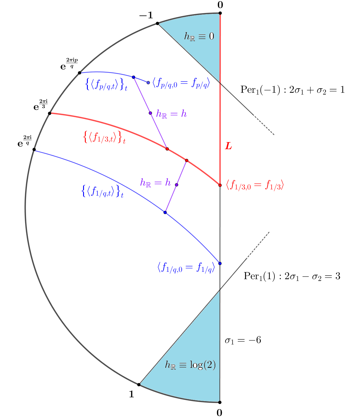
Consider the compactification $\overline{\mathcal{M}_{2}(\mathbb{R})}\cong\overline{\mathbb{D}}$ of the real moduli space introduced in Proposition 2.2 which was formed by adding the circle at infinity (2.9). A portion of $\overline{\mathcal{M}_{2}(\mathbb{R})}$ encompassing the region of $(+-+)$ -bimodal maps is illustrated in Figure 8. The right boundary of this region is the vertical line $\sigma_{1}=-6$ which is the locus where one of the critical points is mapped to another; cf. Figure 1. The real entropy is monotonic along this line, and decreases as the other coordinate $\sigma_{2}$ increases; see Lemma 4.2 and Figure 9 below. In the construction of Proposition 3.2, note that $f_{p/q}$ belongs to this line if $p=1$ . In particular, the classes $\left\langle f_{1/3}\right\rangle$ and $\left\langle f_{1/q}\right\rangle$ lie on this line. In contrast, a point such as $\left\langle f_{p/q}\right\rangle$ where $p/q\in(1/3,1/2)$ does not belong to the line $\sigma_{1}=-6$ as the numerator is different from $1$ ; cf. Proposition 3.2, statement f. Such a numerator $p$ exists; in fact, if $q$ is larger than $q_{0}:=12$ we can pick $p$ so that

1/q<1/3<p/q<1/2;

see Lemma 4.4 below. (Keep in mind that in working with unmarked components $\mathcal{H}_{p/q}$ we take the fraction to be in $(0,1/2)$ ; cf. Convention 3.6.) Fixing such a $p$ , we consider the disjoint curves $\left\{\langle f_{1/q,t}\rangle\right\}_{t\in[0,1)}$ , $\left\{\langle f_{p/q,t}\rangle\right\}_{t\in[0,1)}$ and $\left\{\langle f_{1/3,t}\rangle\right\}_{t\in[0,1)}$ in the corresponding hyperbolic components. The entropy is constant along these curves with $h_{\mathbb{R}}\equiv h_{q}$ along the former two and $h_{\mathbb{R}}\equiv h_{3}$ along the third one. They start at the points $\langle f_{1/q}\rangle$ , $\langle f_{p/q}\rangle$ and $\langle f_{1/3}\rangle$ and, by Proposition 3.9, as $t\uparrow 1$ tend to limit points ${\rm{e}}^{\frac{2\pi{\rm{i}}}{q}}$ , ${\rm{e}}^{\frac{2\pi{\rm{i}}p}{q}}$ and ${\rm{e}}^{\frac{2\pi{\rm{i}}}{3}}$ respectively. Now form the subset $L$ of $\mathcal{M}_{2}(\mathbb{R})$ comprising of the part of the line $\sigma_{1}=-6$ that lies above $\langle f_{1/3}\rangle$ along with the curve $\left\{\langle f_{1/3,t}\rangle\right\}_{t\in[0,1)}$ . Due to the monotonicity along $\sigma_{1}=-6$ , the values that $h_{\mathbb{R}}$ attains on $L$ belong to $\left[0,h^{\prime}=h_{3}\right]$ ; thus $L$ does not intersect the isentrope $h_{\mathbb{R}}=h$ . The closure of $L$ in the closed disk $\overline{\mathcal{M}_{2}(\mathbb{R})}$ touches the boundary circle at two points; and its complement in $\mathcal{M}_{2}(\mathbb{R})$ admits two connected components; see Figure 8. The isentrope $h_{\mathbb{R}}=h$ is contained in this complement, and it suffices to show it has points in both components. The curves $\left\{\langle f_{1/q,t}\rangle\right\}_{t\in[0,1)}$ and $\left\{\langle f_{p/q,t}\rangle\right\}_{t\in[0,1)}$ lie in different connected components of $\mathcal{M}_{2}(\mathbb{R})-L$ due to the fact that, according to the way $p$ was chosen, the corresponding limit points ${\rm{e}}^{\frac{2\pi{\rm{i}}}{q}}$ and ${\rm{e}}^{\frac{2\pi{\rm{i}}p}{q}}$ of them on the boundary circle are located on different sides of the limit point ${\rm{e}}^{\frac{2\pi{\rm{i}}}{3}}$ of $\left\{\langle f_{1/3,t}\rangle\right\}_{t\in[0,1)}$ . Connect points from the former two curves to the latter curve via line segments arbitrarily (as in Figure 8). The interiors of the segments are in different components of $\mathcal{M}_{2}(\mathbb{R})-L$ , and the value $h\in\left(h^{\prime},h_{q}\right]$ is realized by $h_{\mathbb{R}}$ on them by a simple application of the intermediate value theorem. This concludes the proof.

∎

We conclude the paper with the lemmas alluded to during the proof.

Lemma 4.1.

For any $q\geq 3$ the polynomial

(4.1)

P_{q}(t)=t^{q}-2t^{q-1}+1

has a unique root $r_{q}$ in the interval $(1,2)$ . This is the largest positive root of $P_{q}$ and moreover, $\left\{r_{q}\right\}_{q=3}^{\infty}$ is an strictly increasing sequence tending to $2$ .

Proof.

First notice that $P^{\prime}_{q}(t)=qt^{q-1}-2(q-1)t^{q-2}=t^{q-2}\left(qt-2(q-1)\right)$ ; so $c_{q}:=\frac{2(q-1)}{q}>1$ is the only non-zero critical point. The function $P_{q}$ varies as

$t$	$-\infty$		$0$		$1$		$c_{q}$		$2$		$+\infty$
$P_{q}(t)$	$-\infty$	$\nearrow$	$1$	$\searrow$	$0$	$\searrow$	$P_{q}(c_{q})$	$\nearrow$	$1$	$\nearrow$	$+\infty$

when $q$ is odd, and as

$t$	$-\infty$		$0$		$1$		$c_{q}$		$2$		$+\infty$
$P_{q}(t)$	$+\infty$	$\searrow$	$1$	$\searrow$	$0$	$\searrow$	$P_{q}(c_{q})$	$\nearrow$	$1$	$\nearrow$	$+\infty$

for $q$ even. We deduce that $P_{q}(c_{q})<0$ and $P_{q}$ has a unique root $r_{q}$ different from $1$ which lies in $\left(c_{q}=\frac{2(q-1)}{q},2\right)\subset(1,2)$ . We deduce that $\lim_{q\to\infty}r_{q}=2$ . The only thing left to verify is the inequality $r_{q}<r_{q+1}$ . Assume otherwise: $r_{q}\geq r_{q+1}$ . But then $r_{q}\geq r_{q+1}>c_{q+1}>c_{q}$ , and we know that $P_{q}$ is strictly increasing on $(c_{q},+\infty)$ . Thus

(r_{q+1})^{q}-2(r_{q+1})^{q-1}+1=P_{q}(r_{q+1})\leq P_{q}(r_{q})=0.

Multiplying both sides of the inequality above by $r_{q+1}$ , we get

(r_{q+1})^{q+1}-2(r_{q+1})^{q}+r_{q+1}\leq 0.

On the other hand, $P_{q+1}(r_{q+1})=(r_{q+1})^{q+1}-2(r_{q+1})^{q}+1=0$ . It follows immediately that $r_{q+1}\leq 1$ , a contradiction to $r_{q+1}\in(1,2)$ . ∎

Lemma 4.2.

Restricted to the line $\sigma_{1}=-6$ – characterized by the post-critical condition $c_{0}\mapsto c_{1}$ – of the real moduli space, the real entropy is a decreasing function of the other coordinate $\sigma_{2}$ . (The corresponding real entropy graph and the complex bifurcation locus could be found in Figure 9 and [Mil93, Figure 13].)

Proof.

The main idea is to parametrize the conjugacy classes along $\sigma_{1}=-6$ by representatives of the form $a\cdot f_{0}$ , where $f_{0}$ is an appropriate map and $a\in\mathbb{R}$ lies in some suitable interval; and then use the literature on the monotonicity of entropy for one-dimensional families in this form. Up to conjugacy, real quadratic rational maps with the post-critical condition $c_{0}\mapsto c_{1}$ are in the form of $b+\frac{1}{z^{2}}$ where $b\in\mathbb{R}$ . Invoking the formulas derived in [Mil93, Appendix C], the $(\sigma_{1},\sigma_{2})$ -coordinates of the corresponding points of $\mathcal{M}_{2}(\mathbb{R})$ are given by $\sigma_{1}=-6$ and $\sigma_{2}=4b^{3}+12$ . For $b\geq 0$ the topological entropy of $x\in\hat{\mathbb{R}}\mapsto b+\frac{1}{x^{2}}\in\hat{\mathbb{R}}$ is zero due to the fact that the points in $(-\infty,0)$ are wandering and the restriction to the invariant interval $[0,+\infty]$ is monotone decreasing. This covers the upper ray starting at $\left\langle\frac{1}{z^{2}}\right\rangle=(-6,12)$ ; cf. Figure 1. At points $\left\langle b+\frac{1}{z^{2}}\right\rangle$ with $b<0$ – which are below $\left\langle\frac{1}{z^{2}}\right\rangle$ – the function $h_{\mathbb{R}}$ eventually becomes positive because the maps belong to the $h_{\mathbb{R}}\equiv\log(2)$ real escape component provided that $b\ll 0$ . The linear change of coordinates $x\mapsto\sqrt{-b}x$ results in the conjugate maps $z\mapsto a\left(-1+\frac{1}{x^{2}}\right)$ where $a:=\left(\sqrt{-b}\right)^{3}$ . For $a>0$ the image of the map

x\in\hat{\mathbb{R}}\mapsto a\left(-1+\frac{1}{x^{2}}\right)\in\hat{\mathbb{R}}

is the interval $[-a,+\infty]$ which contains only one critical point, $x=0$ . Therefore, one needs to establish the monotonicity of entropy for the family

\left\{x\mapsto a\left(-1+\frac{1}{x^{2}}\right):[-a,+\infty]\rightarrow[-a,+\infty]\right\}_{a>0}

of unimodal interval maps. This immediately follows from [LSv19, Theorem 7.2]. ∎

Remark 4.3.

The line $\sigma_{1}=-6$ is dynamically significant because it is the locus where $c_{0}\mapsto c_{1}$ . By contrast, the entropy fails to be monotonic along arbitrary vertical lines $\sigma_{1}=a$ with $a\ll 0$ since such a line intersects disjoint unbounded hyperbolic components of the form $\mathcal{H}_{1/q}$ and $\mathcal{H}_{p/q}$ which are of the same real entropy value.

Lemma 4.4.

For any $q>12$ there exists an integer $p$ coprime to $q$ satisfying

1/3<p/q<1/2.

Proof.

The desired integer $p$ must be larger than $q/3$ and smaller than $q/2$ . For $q$ odd one can set $p=(q-1)/2$ which is larger than $q/3$ provided that $q>3$ . If $q\equiv 2\pmod{4}$ , the integer $p:=q/2-2$ is coprime to $q$ . It is larger than $q/3$ provided that $q>12$ . Finally, in the case of $q\equiv 0\pmod{4}$ , one can choose $p:=q/2-1$ which satisfies $\gcd(p,q)=1$ , and also $p>q/3$ when $q>6$ . ∎

References

[BK92] L. Block and J. Keesling. Computing the topological entropy of maps of the interval with three monotone pieces. J. Statist. Phys., 66(3-4):755–774, 1992.
[BKLP89] L. Block, J. Keesling, S. Li, and K. Peterson. An improved algorithm for computing topological entropy. J. Statist. Phys., 55(5-6):929–939, 1989.
[BvS15] H. Bruin and S. van Strien. Monotonicity of entropy for real multimodal maps. J. Amer. Math. Soc., 28(1):1–61, 2015.
[DGMT95] S. P. Dawson, R. Galeeva, J. W. Milnor, and C. Tresser. A monotonicity conjecture for real cubic maps. In Real and complex dynamical systems (Hillerød, 1993), volume 464 of NATO Adv. Sci. Inst. Ser. C Math. Phys. Sci., pages 165–183. Kluwer Acad. Publ., Dordrecht, 1995.
[DH85] A. Douady and J. H. Hubbard. Étude dynamique des polynômes complexes. I& II. Publications Mathématiques d’Orsay. 1984,1985.
[DH93] A. Douady and J. H. Hubbard. A proof of Thurston’s topological characterization of rational functions. Acta Math., 171(2):263–297, 1993.
[Dou95] A. Douady. Topological entropy of unimodal maps: monotonicity for quadratic polynomials. In Real and complex dynamical systems (Hillerød, 1993), volume 464 of NATO Adv. Sci. Inst. Ser. C Math. Phys. Sci., pages 65–87. Kluwer Acad. Publ., Dordrecht, 1995.
[Eps00] A. L. Epstein. Bounded hyperbolic components of quadratic rational maps. Ergodic Theory Dynam. Systems, 20(3):727–748, 2000.
[Fil18] K. Filom. Real entropy rigidity under quasi-conformal deformations. arXiv e-prints, page arXiv:1803.04082v2, Mar 2018.
[Fil19] K. Filom. Monotonicity of entropy for real quadratic rational maps. arXiv e-prints, page arXiv:1901.03458v1, Jan 2019.
[Koz19] O. Kozlovski. On the structure of isentropes of real polynomials. J. Lond. Math. Soc. (2), 100(1):159–182, 2019.
[LSv19] G. Levin, W. Shen, and S. van Strien. Positive Transversality via transfer operators and holomorphic motions with applications to monotonicity for interval maps. arXiv e-prints, page arXiv:1902.06732v2, Jan 2019.
[Mil93] J. W. Milnor. Geometry and dynamics of quadratic rational maps. Experiment. Math., 2(1):37–83, 1993. With an appendix by the author and Lei Tan.
[Mil00] J. W. Milnor. On rational maps with two critical points. Experiment. Math., 9(4):481–522, 2000.
[Mil06] J. W. Milnor. Dynamics in one complex variable, volume 160 of Annals of Mathematics Studies. Princeton University Press, Princeton, NJ, third edition, 2006.
[Mil12] J. W. Milnor. Hyperbolic components. In Conformal dynamics and hyperbolic geometry, volume 573 of Contemp. Math., pages 183–232. Amer. Math. Soc., Providence, RI, 2012. With an appendix by A. Poirier.
[Mis95] M. Misiurewicz. Continuity of entropy revisited. In Dynamical systems and applications, volume 4 of World Sci. Ser. Appl. Anal., pages 495–503. World Sci. Publ., River Edge, NJ, 1995.
[MnSS83] R. Mañé, P. Sad, and D. Sullivan. On the dynamics of rational maps. Ann. Sci. École Norm. Sup. (4), 16(2):193–217, 1983.
[MT88] J. W. Milnor and W. P. Thurston. On iterated maps of the interval. In Dynamical systems (College Park, MD, 1986–87), volume 1342 of Lecture Notes in Math., pages 465–563. Springer, Berlin, 1988.
[MT00] J. W. Milnor and C. Tresser. On entropy and monotonicity for real cubic maps. Comm. Math. Phys., 209(1):123–178, 2000. With an appendix by A. Douady and P. Sentenac.
[Pet93] C. L. Petersen. On the Pommerenke-Levin-Yoccoz inequality. Ergodic Theory Dynam. Systems, 13(4):785–806, 1993.
[Pil94] K. M. Pilgrim. Cylinders for iterated rational maps. ProQuest LLC, Ann Arbor, MI, 1994. Thesis (Ph.D.)–University of California, Berkeley.
[Pil96] K. M. Pilgrim. Rational maps whose Fatou components are Jordan domains. Ergodic Theory Dynam. Systems, 16(6):1323–1343, 1996.
[PT98] K. M. Pilgrim and Lei Tan. Combining rational maps and controlling obstructions. Ergodic Theory Dynam. Systems, 18(1):221–245, 1998.
[Ree90] M. Rees. Components of degree two hyperbolic rational maps. Invent. Math., 100(2):357–382, 1990.
[Tan02] Lei Tan. On pinching deformations of rational maps. Ann. Sci. École Norm. Sup. (4), 35(3):353–370, 2002.
[vS14] S. van Strien. Milnor’s conjecture on monotonicity of topological entropy: results and questions. In Frontiers in complex dynamics, volume 51 of Princeton Math. Ser., pages 323–337. Princeton Univ. Press, Princeton, NJ, 2014.

On the Non-monotonicity of entropy for a class of real quadratic rational maps

Abstract.

1. Introduction

Theorem 1.1.

2. Background on the Moduli Space and Hyperbolic Components of Quadratic Rational Maps

Remark 2.1.

Proposition 2.2.

Remark 2.3.

Convention 2.4.

3. Constructing Unbounded Hyperbolic Components ℋp/q\mathcal{H}_{p/q}

Convention 3.1.

Proposition 3.2.

Proof.

Lemma 3.3.

Proof.

Remark 3.4.

Remark 3.5.

Convention-Proposition 3.6.

Proof.

Example 3.7.

Proposition 3.8.

Proof.

Proposition 3.9.

Proof.

Remark 3.10.

4. Proof of the Main Theorem

Proof of Theorem 1.1.

Lemma 4.1.

Proof.

Lemma 4.2.

Proof.

Remark 4.3.

Lemma 4.4.

Proof.

References

3. Constructing Unbounded Hyperbolic Components $\mathcal{H}_{p/q}$