A geometric representation of fragmentation processes
on stable trees
Abstract
We provide a new geometric representation of a family of fragmentation processes by nested laminations, which are compact subsets of the unit disk made of noncrossing chords. We specifically consider a fragmentation obtained by cutting a random stable tree at random points, which split the tree into smaller subtrees. When coding each of these cutpoints by a chord in the unit disk, we separate the disk into smaller connected components, corresponding to the smaller subtrees of the initial tree. This geometric point of view allows us in particular to highlight a new relation between the Aldous-Pitman fragmentation of the Brownian continuum random tree and minimal factorizations of the -cycle, i.e. factorizations of the permutation into a product of transpositions. We discuss various properties of these new lamination-valued processes, and we notably show that they can be coded by explicit Lévy processes.
Twidth 54.44461pt height 6.44444pt depth 1.94444pt/Subtype/Widget/F 2/FT/Btn/Ff 65537/BS <</W 0>>/AP <</N 0 0 R>>/MK <</TP 1/I 0 0 R/IF<</S/A/FB true>>>>/T (0.0)width 54.44461pt height 6.44444pt depth 1.94444pt/Subtype/Widget/F 2/FT/Btn/Ff 65537/BS <</W 0>>/AP <</N 0 0 R>>/MK <</TP 1/I 0 0 R/IF<</S/A/FB true>>>>/T (0.1)width 54.44461pt height 6.44444pt depth 1.94444pt/Subtype/Widget/F 2/FT/Btn/Ff 65537/BS <</W 0>>/AP <</N 0 0 R>>/MK <</TP 1/I 0 0 R/IF<</S/A/FB true>>>>/T (0.2)width 54.44461pt height 6.44444pt depth 1.94444pt/Subtype/Widget/F 2/FT/Btn/Ff 65537/BS <</W 0>>/AP <</N 0 0 R>>/MK <</TP 1/I 0 0 R/IF<</S/A/FB true>>>>/T (0.3)width 54.44461pt height 6.44444pt depth 1.94444pt/Subtype/Widget/F 2/FT/Btn/Ff 65537/BS <</W 0>>/AP <</N 0 0 R>>/MK <</TP 1/I 0 0 R/IF<</S/A/FB true>>>>/T (0.4)width 54.44461pt height 6.44444pt depth 1.94444pt/Subtype/Widget/F 2/FT/Btn/Ff 65537/BS <</W 0>>/AP <</N 0 0 R>>/MK <</TP 1/I 0 0 R/IF<</S/A/FB true>>>>/T (0.5)width 54.44461pt height 6.44444pt depth 1.94444pt/Subtype/Widget/F 2/FT/Btn/Ff 65537/BS <</W 0>>/AP <</N 0 0 R>>/MK <</TP 1/I 0 0 R/IF<</S/A/FB true>>>>/T (0.6)width 54.44461pt height 6.44444pt depth 1.94444pt/Subtype/Widget/F 2/FT/Btn/Ff 65537/BS <</W 0>>/AP <</N 0 0 R>>/MK <</TP 1/I 0 0 R/IF<</S/A/FB true>>>>/T (0.7)width 54.44461pt height 6.44444pt depth 1.94444pt/Subtype/Widget/F 2/FT/Btn/Ff 65537/BS <</W 0>>/AP <</N 0 0 R>>/MK <</TP 1/I 0 0 R/IF<</S/A/FB true>>>>/T (0.8)width 54.44461pt height 6.44444pt depth 1.94444pt/Subtype/Widget/F 2/FT/Btn/Ff 65537/BS <</W 0>>/AP <</N 0 0 R>>/MK <</TP 1/I 0 0 R/IF<</S/A/FB true>>>>/T (0.9)width 54.44461pt height 6.44444pt depth 1.94444pt/Subtype/Widget/F 2/FT/Btn/Ff 65537/BS <</W 0>>/AP <</N 0 0 R>>/MK <</TP 1/I 0 0 R/IF<</S/A/FB true>>>>/T (0.10)width 54.44461pt height 6.44444pt depth 1.94444pt/Subtype/Widget/F 2/FT/Btn/Ff 65537/BS <</W 0>>/AP <</N 0 0 R>>/MK <</TP 1/I 0 0 R/IF<</S/A/FB true>>>>/T (0.11)width 54.44461pt height 6.44444pt depth 1.94444pt/Subtype/Widget/F 2/FT/Btn/Ff 65537/BS <</W 0>>/AP <</N 0 0 R>>/MK <</TP 1/I 0 0 R/IF<</S/A/FB true>>>>/T (0.12)width 54.44461pt height 6.44444pt depth 1.94444pt/Subtype/Widget/F 2/FT/Btn/Ff 65537/BS <</W 0>>/AP <</N 0 0 R>>/MK <</TP 1/I 0 0 R/IF<</S/A/FB true>>>>/T (0.13)width 54.44461pt height 6.44444pt depth 1.94444pt/Subtype/Widget/F 2/FT/Btn/Ff 65537/BS <</W 0>>/AP <</N 0 0 R>>/MK <</TP 1/I 0 0 R/IF<</S/A/FB true>>>>/T (0.14)width 54.44461pt height 6.44444pt depth 1.94444pt/Subtype/Widget/F 2/FT/Btn/Ff 65537/BS <</W 0>>/AP <</N 0 0 R>>/MK <</TP 1/I 0 0 R/IF<</S/A/FB true>>>>/T (0.15)width 54.44461pt height 6.44444pt depth 1.94444pt/Subtype/Widget/F 2/FT/Btn/Ff 65537/BS <</W 0>>/AP <</N 0 0 R>>/MK <</TP 1/I 0 0 R/IF<</S/A/FB true>>>>/T (0.16)width 54.44461pt height 6.44444pt depth 1.94444pt/Subtype/Widget/F 2/FT/Btn/Ff 65537/BS <</W 0>>/AP <</N 0 0 R>>/MK <</TP 1/I 0 0 R/IF<</S/A/FB true>>>>/T (0.17)width 54.44461pt height 6.44444pt depth 1.94444pt/Subtype/Widget/F 2/FT/Btn/Ff 65537/BS <</W 0>>/AP <</N 0 0 R>>/MK <</TP 1/I 0 0 R/IF<</S/A/FB true>>>>/T (0.18)width 54.44461pt height 6.44444pt depth 1.94444pt/Subtype/Widget/F 2/FT/Btn/Ff 65537/BS <</W 0>>/AP <</N 0 0 R>>/MK <</TP 1/I 0 0 R/IF<</S/A/FB true>>>>/T (0.19)width 54.44461pt height 6.44444pt depth 1.94444pt/Subtype/Widget/F 2/FT/Btn/Ff 65537/BS <</W 0>>/AP <</N 0 0 R>>/MK <</TP 1/I 0 0 R/IF<</S/A/FB true>>>>/T (0.20)width 54.44461pt height 6.44444pt depth 1.94444pt/Subtype/Widget/F 2/FT/Btn/Ff 65537/BS <</W 0>>/AP <</N 0 0 R>>/MK <</TP 1/I 0 0 R/IF<</S/A/FB true>>>>/T (0.21)width 54.44461pt height 6.44444pt depth 1.94444pt/Subtype/Widget/F 2/FT/Btn/Ff 65537/BS <</W 0>>/AP <</N 0 0 R>>/MK <</TP 1/I 0 0 R/IF<</S/A/FB true>>>>/T (0.22)width 54.44461pt height 6.44444pt depth 1.94444pt/Subtype/Widget/F 2/FT/Btn/Ff 65537/BS <</W 0>>/AP <</N 0 0 R>>/MK <</TP 1/I 0 0 R/IF<</S/A/FB true>>>>/T (0.23)width 54.44461pt height 6.44444pt depth 1.94444pt/Subtype/Widget/F 2/FT/Btn/Ff 65537/BS <</W 0>>/AP <</N 0 0 R>>/MK <</TP 1/I 0 0 R/IF<</S/A/FB true>>>>/T (0.24)width 54.44461pt height 6.44444pt depth 1.94444pt/Subtype/Widget/F 2/FT/Btn/Ff 65537/BS <</W 0>>/AP <</N 0 0 R>>/MK <</TP 1/I 0 0 R/IF<</S/A/FB true>>>>/T (0.25)width 54.44461pt height 6.44444pt depth 1.94444pt/Subtype/Widget/F 2/FT/Btn/Ff 65537/BS <</W 0>>/AP <</N 0 0 R>>/MK <</TP 1/I 0 0 R/IF<</S/A/FB true>>>>/T (0.26)width 54.44461pt height 6.44444pt depth 1.94444pt/Subtype/Widget/F 2/FT/Btn/Ff 65537/BS <</W 0>>/AP <</N 0 0 R>>/MK <</TP 1/I 0 0 R/IF<</S/A/FB true>>>>/T (0.27)width 54.44461pt height 6.44444pt depth 1.94444pt/Subtype/Widget/F 2/FT/Btn/Ff 65537/BS <</W 0>>/AP <</N 0 0 R>>/MK <</TP 1/I 0 0 R/IF<</S/A/FB true>>>>/T (0.28)width 54.44461pt height 6.44444pt depth 1.94444pt/Subtype/Widget/F 2/FT/Btn/Ff 65537/BS <</W 0>>/AP <</N 0 0 R>>/MK <</TP 1/I 0 0 R/IF<</S/A/FB true>>>>/T (0.29)width 54.44461pt height 6.44444pt depth 1.94444pt/Subtype/Widget/F 2/FT/Btn/Ff 65537/BS <</W 0>>/AP <</N 0 0 R>>/MK <</TP 1/I 0 0 R/IF<</S/A/FB true>>>>/T (0.30)width 54.44461pt height 6.44444pt depth 1.94444pt/Subtype/Widget/F 2/FT/Btn/Ff 65537/BS <</W 0>>/AP <</N 0 0 R>>/MK <</TP 1/I 0 0 R/IF<</S/A/FB true>>>>/T (0.31)width 54.44461pt height 6.44444pt depth 1.94444pt/Subtype/Widget/F 2/FT/Btn/Ff 65537/BS <</W 0>>/AP <</N 0 0 R>>/MK <</TP 1/I 0 0 R/IF<</S/A/FB true>>>>/T (0.32)width 54.44461pt height 6.44444pt depth 1.94444pt/Subtype/Widget/F 2/FT/Btn/Ff 65537/BS <</W 0>>/AP <</N 0 0 R>>/MK <</TP 1/I 0 0 R/IF<</S/A/FB true>>>>/T (0.33)width 54.44461pt height 6.44444pt depth 1.94444pt/Subtype/Widget/F 2/FT/Btn/Ff 65537/BS <</W 0>>/AP <</N 0 0 R>>/MK <</TP 1/I 0 0 R/IF<</S/A/FB true>>>>/T (0.34)width 54.44461pt height 6.44444pt depth 1.94444pt/Subtype/Widget/F 2/FT/Btn/Ff 65537/BS <</W 0>>/AP <</N 0 0 R>>/MK <</TP 1/I 0 0 R/IF<</S/A/FB true>>>>/T (0.35)width 54.44461pt height 6.44444pt depth 1.94444pt/Subtype/Widget/F 2/FT/Btn/Ff 65537/BS <</W 0>>/AP <</N 0 0 R>>/MK <</TP 1/I 0 0 R/IF<</S/A/FB true>>>>/T (0.36)width 54.44461pt height 6.44444pt depth 1.94444pt/Subtype/Widget/F 2/FT/Btn/Ff 65537/BS <</W 0>>/AP <</N 0 0 R>>/MK <</TP 1/I 0 0 R/IF<</S/A/FB true>>>>/T (0.37)width 54.44461pt height 6.44444pt depth 1.94444pt/Subtype/Widget/F 2/FT/Btn/Ff 65537/BS <</W 0>>/AP <</N 0 0 R>>/MK <</TP 1/I 0 0 R/IF<</S/A/FB true>>>>/T (0.38)width 54.44461pt height 6.44444pt depth 1.94444pt/Subtype/Widget/F 2/FT/Btn/Ff 65537/BS <</W 0>>/AP <</N 0 0 R>>/MK <</TP 1/I 0 0 R/IF<</S/A/FB true>>>>/T (0.39)width 54.44461pt height 6.44444pt depth 1.94444pt/Subtype/Widget/F 2/FT/Btn/Ff 65537/BS <</W 0>>/AP <</N 0 0 R>>/MK <</TP 1/I 0 0 R/IF<</S/A/FB true>>>>/T (0.40)width 54.44461pt height 6.44444pt depth 1.94444pt/Subtype/Widget/F 2/FT/Btn/Ff 65537/BS <</W 0>>/AP <</N 0 0 R>>/MK <</TP 1/I 0 0 R/IF<</S/A/FB true>>>>/T (0.41)width 54.44461pt height 6.44444pt depth 1.94444pt/Subtype/Widget/F 2/FT/Btn/Ff 65537/BS <</W 0>>/AP <</N 0 0 R>>/MK <</TP 1/I 0 0 R/IF<</S/A/FB true>>>>/T (0.42)width 54.44461pt height 6.44444pt depth 1.94444pt/Subtype/Widget/F 2/FT/Btn/Ff 65537/BS <</W 0>>/AP <</N 0 0 R>>/MK <</TP 1/I 0 0 R/IF<</S/A/FB true>>>>/T (0.43)width 54.44461pt height 6.44444pt depth 1.94444pt/Subtype/Widget/F 2/FT/Btn/Ff 65537/BS <</W 0>>/AP <</N 0 0 R>>/MK <</TP 1/I 0 0 R/IF<</S/A/FB true>>>>/T (0.44)width 54.44461pt height 6.44444pt depth 1.94444pt/Subtype/Widget/F 2/FT/Btn/Ff 65537/BS <</W 0>>/AP <</N 0 0 R>>/MK <</TP 1/I 0 0 R/IF<</S/A/FB true>>>>/T (0.45)width 54.44461pt height 6.44444pt depth 1.94444pt/Subtype/Widget/F 2/FT/Btn/Ff 65537/BS <</W 0>>/AP <</N 0 0 R>>/MK <</TP 1/I 0 0 R/IF<</S/A/FB true>>>>/T (0.46)width 54.44461pt height 6.44444pt depth 1.94444pt/Subtype/Widget/F 2/FT/Btn/Ff 65537/BS <</W 0>>/AP <</N 0 0 R>>/MK <</TP 1/I 0 0 R/IF<</S/A/FB true>>>>/T (0.47)width 54.44461pt height 6.44444pt depth 1.94444pt/Subtype/Widget/F 2/FT/Btn/Ff 65537/BS <</W 0>>/AP <</N 0 0 R>>/MK <</TP 1/I 0 0 R/IF<</S/A/FB true>>>>/T (0.48)width 54.44461pt height 6.44444pt depth 1.94444pt/Subtype/Widget/F 2/FT/Btn/Ff 65537/BS <</W 0>>/AP <</N 0 0 R>>/MK <</TP 1/I 0 0 R/IF<</S/A/FB true>>>>/T (0.49)width 54.44461pt height 6.44444pt depth 1.94444pt/Subtype/Widget/F 2/FT/Btn/Ff 65537/BS <</W 0>>/AP <</N 0 0 R>>/MK <</TP 1/I 0 0 R/IF<</S/A/FB true>>>>/T (0.50) width 1ex height 1ex depth /Subtype/Screen/F 2/AA <</PV <</S/JavaScript/JS 0 0 R>>/PO <</S/JavaScript/JS 0 0 R>>/PI <</S/JavaScript/JS 0 0 R>>/PC <</S/JavaScript/JS 0 0 R>>>>width 54.44461pt height 6.44444pt depth 1.94444pt/Subtype/Widget/FT/Btn/Ff 65536/F 4/BS <</W 0>>/H/N/T (anm0)/Contents (animation by animate, v. 2023/06/18)/AA <</PV <</S/JavaScript/JS 0 0 R>>/PO <</S/JavaScript/JS 0 0 R>>/PI <</S/JavaScript/JS 0 0 R>>/PC <</S/JavaScript/JS 0 0 R>>/D <</S/JavaScript/JS (tryif(a0_playing)a0_pause();catch(e))>>/U <</S/JavaScript/JS (tryif(event.shift)a0_playsRight=!a0_playsRight;var doplay=true;if(a0_idx==50a0_playsRight)a0_stopFirst();if(a0_idx==0!a0_playsRight)a0_stopLast();if(doplay)if(a0_playsRight)a0_playRight();elsea0_playLeft();catch(e))>>>>/AP <</N 0 0 R>>/MK <</TP 1/I 0 0 R/IF<</S/A/FB true>>>> \pdfxformTwidth 14.40004pt height 14.40004pt depth /Subtype/Widget/F 0/FT/Btn/Ff 65536/H/I/BS <</W 0>>/AP <</N 0 0 R>>/MK <</TP 1/I 0 0 R/IF<</S/A/FB true>>>>/T (0.EndLeft)/AA <</D <</S/JavaScript/JS (a0_stopFirst();)>>>>\pdfxformTwidth 14.40004pt height 14.40004pt depth /Subtype/Widget/F 0/FT/Btn/Ff 65536/H/I/BS <</W 0>>/AP <</N 0 0 R>>/MK <</TP 1/I 0 0 R/IF<</S/A/FB true>>>>/T (0.StepLeft)/AA <</D <</S/JavaScript/JS (a0_stepBwd();)>>>>\pdfxformTwidth 14.40004pt height 14.40004pt depth /Subtype/Widget/F 2/FT/Btn/Ff 65537/H/N/BS <</W 0>>/AP <</N 0 0 R>>/MK <</TP 1/I 0 0 R/IF<</S/A/FB true>>>>/T (0.PauseLeft)\pdfxformTwidth 14.40004pt height 14.40004pt depth /Subtype/Widget/F 0/FT/Btn/Ff 65537/H/N/BS <</W 0>>/AP <</N 0 0 R>>/MK <</TP 1/I 0 0 R/IF<</S/A/FB true>>>>/T (0.PlayLeft)\pdfxformTwidth 14.40004pt height 14.40004pt depth /Subtype/Widget/F 0/FT/Btn/Ff 65536/H/I/BS <</W 0>>/AP <</N 0 0 R>>/MK <</TP 1/I 0 0 R/IF<</S/A/FB true>>>>/T (0.PlayPauseLeft)/AA <</D <</S/JavaScript/JS (a0_playPauseBwd();)>>>>\pdfxformTwidth 14.40004pt height 14.40004pt depth /Subtype/Widget/F 2/FT/Btn/Ff 65537/H/N/BS <</W 0>>/AP <</N 0 0 R>>/MK <</TP 1/I 0 0 R/IF<</S/A/FB true>>>>/T (0.PauseRight)\pdfxformTwidth 14.40004pt height 14.40004pt depth /Subtype/Widget/F 0/FT/Btn/Ff 65537/H/N/BS <</W 0>>/AP <</N 0 0 R>>/MK <</TP 1/I 0 0 R/IF<</S/A/FB true>>>>/T (0.PlayRight)width 14.40004pt height 14.40004pt depth /Subtype/Widget/F 0/FT/Btn/Ff 65536/H/I/BS <</W 0>>/AP <</N 0 0 R>>/MK <</TP 1/I 0 0 R/IF<</S/A/FB true>>>>/T (0.PlayPauseRight)/AA <</D <</S/JavaScript/JS (a0_playPauseFwd();)>>>>\pdfxformTwidth 14.40004pt height 14.40004pt depth /Subtype/Widget/F 0/FT/Btn/Ff 65536/H/I/BS <</W 0>>/AP <</N 0 0 R>>/MK <</TP 1/I 0 0 R/IF<</S/A/FB true>>>>/T (0.StepRight)/AA <</D <</S/JavaScript/JS (a0_stepFwd();)>>>>\pdfxformTwidth 14.40004pt height 14.40004pt depth /Subtype/Widget/F 0/FT/Btn/Ff 65536/H/I/BS <</W 0>>/AP <</N 0 0 R>>/MK <</TP 1/I 0 0 R/IF<</S/A/FB true>>>>/T (0.EndRight)/AA <</D <</S/JavaScript/JS (a0_stopLast();)>>>> \pdfxformTwidth 14.40004pt height 14.40004pt depth /Subtype/Widget/F 0/FT/Btn/Ff 65536/H/I/BS <</W 0>>/AP <</N 0 0 R>>/MK <</TP 1/I 0 0 R/IF<</S/A/FB true>>>>/T (0.Minus)/TU (slower)/AA <</D <</S/JavaScript/JS (a0_spdDecr();)>>>>\pdfxformTwidth 14.40004pt height 14.40004pt depth /Subtype/Widget/F 0/FT/Btn/Ff 65536/H/I/BS <</W 0>>/AP <</N 0 0 R>>/MK <</TP 1/I 0 0 R/IF<</S/A/FB true>>>>/T (0.Reset)/TU (default speed)/AA <</D <</S/JavaScript/JS (a0_spdReset();)>>>>\pdfxformTwidth 14.40004pt height 14.40004pt depth /Subtype/Widget/F 0/FT/Btn/Ff 65536/H/I/BS <</W 0>>/AP <</N 0 0 R>>/MK <</TP 1/I 0 0 R/IF<</S/A/FB true>>>>/T (0.Plus)/TU (faster)/AA <</D <</S/JavaScript/JS (a0_spdIncr();)>>>>
1 Introduction
The purpose of this work is to investigate a geometric and dynamical representation of fragmentation processes derived from random stable trees in terms of laminations, with an application to permutation factorizations. Specifically, we shall code the analogue of the Aldous-Pitman fragmentation on a stable tree by a new lamination-valued càdlàg process. Also, in the Brownian case, we shall establish a connection between this lamination-valued process and minimal factorizations of a cycle into transpositions. Before stating our results, let us first present the main objects of interest.
1.1 Fragmentations and laminations
Fragmentation processes derived from stable trees.
Fragmentation processes describe the evolution of an object with given mass, which splits into smaller pieces as time passes. Specifically, a fragmentation process is a càdlàg process (that is, left-continuous with right limits) on the set
such that, if one denotes by the law of starting from , then is the nonincreasing reordering of the elements of independent processes of laws . This means that each fragment breaks independently of the others, in a way that only depends on its mass.
The starting point of this paper is a well-known fragmentation process which was introduced by Aldous and Pitman [8] and which consists in cutting a specific random tree - namely, Aldous’ Brownian tree - at random points. These cutpoints are spread out on the tree following a homogeneous Poisson distribution of density , where and is the length measure on the tree. The Brownian tree (sometimes called CRT, for continuum random tree) is therefore split into smaller components as increases. This process has been studied in depth, notably by Bertoin [10] who gives a different surprising construction from a linearly drifted standard Brownian excursion over its current infimum, as the slope of the drift varies. Miermont [47] has considered more generally fragmentations obtained by cutting at random the so-called stable trees. These random trees (for ), introduced by Duquesne and Le Gall [25] (see also [42]), can be coded by -stable spectrally positive Lévy processes and arise as scaling limits of size-conditioned Galton-Watson trees. They generalize Aldous’ Brownian tree, which can be seen as the -stable tree. Miermont investigates a way of cutting these stable trees only at branching points — that is, points whose removal splits the tree into three or more different subtrees –, while Abraham & Serlet [4] cut them uniformly on their skeleton (made of points which are not branching points). This gives birth to two different fragmentation processes. Let us also mention Voisin [54] who studies a mixture of these two processes. Fragmentations can also more generally be derived from Lévy trees (see [1, 3, 4]), which are trees coded by Lévy processes.
Let us briefly mention that a fragmentation process can be seen as a time-reversed coalescent process, where particles with given masses merge at a rate that depends on their respective masses. The so-called standard additive coalescent is the coalescent process where only two particles merge at each time, at a rate that is the sum of their masses. This standard coalescent is the time-reversed analogue of the previously mentioned Aldous-Pitman fragmentation process on the Brownian tree [8]. Several other models of coalescent processes have been investigated, such as Kingman’s coalescent [37] where two particles merge at rate , or Aldous’ multiplicative coalescent [6, 7] where particles merge proportionally to the product of their masses. See also the book of Bertoin [11] for fully detailed information about coalescent processes. Let us finally mention Chassaing and Louchard [18] who provide a representation of the standard additive coalescent as parking schemes (see also [44]).
In this paper, we consider the previously mentioned analogue of the Aldous-Pitman fragmentation on a stable tree. Specifically, we fix and focus on cutting the -stable tree homogeneously on its skeleton by a homogeneous Poisson process of intensity , where and is the length measure on the tree, consistently as increases (we refer to Section 2 for precise definitions, and [9] for a rigorous definition of ). Cutting at the points of then splits the tree into a random set of smaller components, whose decreasingly reordered sequence of masses (i.e., the proportion of leaves of the tree in these components, see again Section 2 for precise definitions) is an element of . This defines the -fragmentation process
In the case , this is the Aldous-Pitman fragmentation of .
Laminations and excursion-type functions.
The aim of this paper is to code the analogue of the Aldous-Pitman fragmentation on a stable tree by a nondecreasing lamination-valued process, where, roughly speaking, a chord in the lamination corresponds to a cutpoint on the tree. By definition, a lamination is a closed subset of the closed unit disk which can be written as the union of the unit circle and a set of chords which do not intersect in the open unit disk . Laminations are important objects in topology and in hyperbolic geometry, see for instance [17] and references therein. If is a lamination, a face of is a connected component of the complement of in .
The connection between random trees and random laminations goes back to Aldous [5] who used the Brownian excursion to code the so-called Brownian triangulation (see Fig. 3, right, for a simulation). The Brownian triangulation is a random lamination whose faces are all triangles, and its “dual” tree is, in some sense, the Brownian CRT. Since then, this object has appeared as the limit of several discrete structures [20, 40, 14], and in the theory of random planar maps [43].
Other models of random laminations have been recently studied. The Brownian triangulation has been generalized by Kortchemski [38], who introduced, for the so-called -stable lamination, whose “dual” tree is in a certain sense the -stable tree, and which appears as the limit of certain models of random dissections (which are collections of noncrossing diagonals of a regular polygon). In a different direction, Curien and Le Gall [21] consider laminations built by recursively adding chords. Another family of random laminations connected to random minimal factorizations of a cycle into transpositions, which will be one of the objects of interest in this paper, has been introduced in [27]. While all these random laminations can be coded by random excursion-type functions, other laminations such as the hyperbolic triangulation [22] or triangulated stable laminations [39] cannot.
Let us immediately explain how to construct laminations from so-called excursion-type functions. Let . We say that is an excursion-type function if the following conditions are verified:
- (i)
is càdlàg (that is, right-continuous on , with left limits on );
- (ii)
is nonnegative on and ;
- (iii)
only makes positive jumps, that is, for all , .
Following the construction of [38], to an excursion-type function , one can associate a lamination as follows. For any , say that if (where we set ). For , we say that if , and we say that for any , . This way, is an equivalence relation on . The lamination is defined as the closure
where denotes the line segment joining the two complex numbers and .
The -stable lamination, which plays an important role in our work, can be constructed from a planar version of the -stable tree (we refer to Section 2.2 for precise definitions). Indeed, we view as coded by a continuous normalized -stable height process (so that, informally, is the contour function of ). We define the -stable lamination as
| (1) |
It is possible to check (see [38]) that faces of are in correspondence with branching points of , and that there are chords which are not adjacent to any face (one can find chords arbitrarily close to such a chord, from both sides) which are in correspondence with the points of that are not leaves nor branching points. See Fig. 2 for an approximation of these items, for .

We conclude this section with a last definition concerning laminations. We define the mass of a face of a lamination as times the Lebesgue measure of (roughly speaking, it corresponds to the part of the perimeter of that lies on the unit circle). Finally, the mass sequence of , denoted by , is the sequence of the masses of its faces, sorted in nonincreasing order.
1.2 The lamination-valued process
For a fixed , we now introduce a new lamination-valued process which encodes, in a certain sense, the fragmentation of the -stable tree. Here we give a rather informal definition, and defer to Section 2 precise definitions.
Definition of .
As above, we view as coded by a normalized -stable height process . We consider a homogeneous Poisson process of intensity on the skeleton of , where and is the length measure on the tree, consistently as increases. For , we define the lamination as the subset of the -stable lamination , obtained by keeping only the chords which correspond to the vertices of (recall that to points of the skeleton of correspond chords of ). Intuitively speaking, one obtains the process by revealing the chords of in a Poissonian way (see Fig. 1 for an approximation of ).
Connection with fragmentations.
The process , which is an increasing lamination-valued process, is the main object of interest in this paper. It encodes the Aldous-Pitman fragmentation of the -stable tree in the following sense (where we recall that is the mass sequence of a lamination ).

Theorem 1.1.
The following equality holds in distribution in :
In a certain sense, can be viewed as a “dual planar representation” of the Aldous-Pitman fragmentation of the -stable tree, and as a “linearization” of the associated time-reversed coalescent process. In order to prove Theorem 1.1, we view the Poissonian cuts on the skeleton of as a non-homogenous Poisson process in the epigraph of (see Section 2.2).
Let us mention that for fixed and , the lamination appears in [27] in the context of random minimal factorizations of a cycle, without any connection to fragmentations. In addition, defining a coupling as increases and obtaining a functional convergence was left open in [27]. Also, Shi [51] used fragmentation theory to study large faces in the Brownian triangulation and in stable laminations, by using the so-called fragmentation by heights of stable trees (which is different from the one that appears here, see [46]).
Also, throughout the paper, the lamination-valued processes will be defined on , while the associated fragmentation processes are only defined on . Observe indeed that, almost surely, as , which corresponds to extinction at . On the other hand, the increasing process has a non-trivial limit at .
1.3 Connections with random minimal factorizations
One of the main contributions of this paper is to show that the process appears as the functional limit of a natural coding of so-called minimal factorizations of the -cycle. More precisely, for , denote by the group of permutations acting on and by the set of transpositions of . Then, the elements of the set
are called minimal factorizations of the -cycle into transpositions, or just minimal factorizations in short. Their study goes back to Dénès [23] and Moszkowski [48]. By convention, we read transpositions from left to right, so that corresponds to .
Goulden and Yong [30] view minimal factorizations in a geometric way, noticing that it is possible to represent each of them by a non-crossing tree in the unit disk. More specifically, if and for , then
is a non-crossing tree and, in particular, a lamination (adding , see Fig. 4). In this direction, for a uniform minimal factorization of the -cycle, Féray and Kortchemski [27] have shown that a phase transition occurs when roughly transpositions have been read. More precisely, for , if is the lamination obtained by drawing the chords corresponding to the first transpositions of , then [27, Theorem , (i)] shows that for , converges in distribution for the Hausdorff distance to a limiting random lamination, defined by using a certain Lévy process (and not fragmentations nor Poisson processes).
One of the main results of this paper is to show that this convergence actually holds in the functional sense (that is, jointly in ) and that the limiting process is . As a corollary, we obtain an alternative and, in our opinion, simpler proof of the one-dimensional convergence [27, Theorem , (i)].
Let us quickly give some background concerning this notion of convergence. The set of laminations of the closed unit disk is endowed with the Hausdorff distance between compact subsets of , so that is a Polish metric space (that is, separable and complete). The Hausdorff distance is defined as follows. If is a compact subset of and , define the -neighbourhood of as , where denotes the usual Euclidean distance on . Then, for compact subsets of the unit disk, we define
In the rest of the paper, for two metric spaces, denotes the set of càdlàg processes from to , endowed with the Skorokhod topology (see Annex in [34] for background). Finally, we denote by the Alexandrov extension of , which is compact by definition.
Theorem 1.2.
The following convergence holds in distribution in :
To establish this result, we actually prove a more general result (Theorem 2.4 below). We show that is the functional limit of discrete lamination valued-processes, obtained by marking vertices of discrete trees (this can be seen as the discrete analogue of the Aldous-Pitman fragmentation). We then use a bijection between the set of minimal factorizations of the -cycle and a subset of plane trees with labelled vertices, which allows us to reformulate Theorem 1.2 in terms of random trees. The main difficulty is that the labelling of the vertices has constraints. To lift these constraints and to reduce the study to uniform labellings, an important tool in the study of these random trees is an operation that shuffles the labels of their vertices in two ways (see Section 4 for details).
The process is therefore the limit of discrete lamination-valued processes which code a uniform minimal factorization into transpositions; in a forthcoming work, we establish an analogous result concerning the processes for , by proving that they appear as limits of discrete lamination-valued processes which code other random factorizations of the -cycle. Notably, cycles of length are allowed in these new models of factorizations.
1.4 Coding by a function
For fixed and , we show that can be coded by a Lévy process, similarly to the way is coded by in (1). In the case of , we introduce the -stable spectrally positive Lévy process , which is the Lévy process whose Laplace exponent is given by for . Then, for any , we define the stopping time as
It is not difficult (see Section 5) to check that is a Lévy process with Laplace exponent given by
where is the unique nonnegative solution of the equation . It is interesting to note that this equation appears in the work of Bertoin [12, Section ], in the study of a random spatial branching process with emigration.
It turns out that can be coded by the normalized excursion of the Lévy process , as stated in the following theorem:
Theorem 1.3.
The following equality holds in distribution, for any :
Here, is the lamination constructed from by the method described in Section 1.1.
The main idea of the proof of Theorem 1.3 is to exhibit a new family of random trees, which can be seen as a randomly reduced version, in some sense, of Galton-Watson trees conditioned by their number of vertices. It happens that these reduced trees code a new sequence of random laminations, which converges at the same time towards and .
1.5 An estimate on generating functions
An important ingredient to code by the normalized excursion of , which is crucial in the proof of Theorem 1.3 and which we believe to be of independent interest, is a general estimate of the behavior of generating functions in the complex plane, involving slowly varying functions. Recall that a function is slowly varying if, for any , as . Precise estimates concerning these functions are needed in many different contexts, see e.g. [52] [53], although nothing seems to have been proved regarding asymptotics in the complex domain.
Theorem 1.4.
Let be a probability distribution on the nonnegative integers and denote by its generating function. Assume that there exists and a slowly varying function such that
Then
In the terminology of Galton-Watson trees, this is an estimate in the complex unit disk, near , of the generating function of a critical offspring distribution which belongs to the domain of attraction of a stable law. Very often, additional assumptions, such as -analyticity, are made in order to obtain estimates for generating functions in the complex plane (see [29, Section 6]). Observe that here it is not the case, and no assumptions on are made.
The proof of this theorem is given in Section 6. The main idea is to use an integral representation, see (30).
Outline
After describing a general construction of trees and laminations coded by excursion-type functions, we rigorously define the process in Section 2 and prove Theorem 1.1. In a second time, in Section 3, we make appear as the limit of a process of laminations coded by discrete trees; this framework is used in Section 4 to extend the results of Féray & Kortchemski [27] and highlight a relation between the Aldous-Pitman fragmentation of the Brownian tree and minimal factorizations of the -cycle as . Finally, in Section 5, we recover the -dimensional marginal of the lamination process as the lamination coded by (Theorem 1.3), while Section 6 is devoted to the proof of Theorem 1.4.
Acknowledgements.
I would like to thank Igor Kortchemski for asking the questions at the origin of this paper and for his help, comments, suggestions and corrections. I would also like to thank Bénédicte Haas, Cyril Marzouk and Loïc Richier for fruitful discussions and comments on the paper, and Gerónimo Uribe Bravo for his useful remarks on Theorem 5.1.
Notations
Let us immediately sum up some notations that will often appear throughout the paper. We write for the convergence in probability, and for the convergence in distribution of a sequence of random variables. We say that an event (depending on ) occurs with high probability if as . When talking about trees, deterministic ones will be denoted by a straight , while random ones will be denoted by a curved . Finally, at the beginning of each section, we sum up the most important notations that we use in this section.
2 Construction of lamination-valued processes
This section is devoted to the construction of càdlàg processes taking their values in the set of laminations of the unit disk. We start by explaining a general method of construction of lamination-valued processes, starting from a deterministic excursion-type function. Then, we apply this in the particular case of an -stable excursion, for , giving birth to a random lamination-valued process.
Notations of Section 2
In this table of notations, always denotes a continuous excursion-type function such that (except for , which is defined for any excursion-type function). denotes an element of .
| epigraph of | |
|---|---|
| Poisson point process of intensity on | |
| Poisson point process of intensity on a tree | |
| lamination coded by | |
| lamination coded by | |
| -stable tree | |
| contour function of the -stable tree | |
| -stable lamination, coded by | |
| lamination coded by |
2.1 Excursions and laminations
Starting from an excursion-type function , we have seen in Section 1 that we can define a lamination . In the particular case of a continuous verifying , we shall recall in this section the classical construction of the tree as the quotient of by the equivalence relation defined in Section 1.1. Then, we shall construct a nondecreasing lamination-valued process , by associating chords in the unit disk to straight lines under the graph of (see Fig. 6), such that . It is to note that, when is deterministic, and are also deterministic, while will be a random process. This coding is used in the next sections, when the function is the contour function of a tree (later in this section and in the next one) or when it is the standard excursion of the Lévy process (Section 5).
The tree associated to continuous excursion-type function.
Assume that is a continuous excursion-type function with . In this case, the equivalence relation defined in Section 1.1 can be understood in a nicer way. For , define and . For , set . For , we write if , which matches the definition of Section 1.1.
From this continuous function , we define the tree as
One can check (see [25]) that induces a distance on , which we still denote by with a slight abuse of notation, and that the metric space is a tree, in the sense that from one point of to another, there exists a unique path in . See Fig. 2 and 3 for two examples of a continuous excursion-type function, its associated lamination and its associated tree.
Let us immediately define some important notions about trees. We say that an equivalence class is a branching point if has at least three disjoint connected components, and the set of points that are not branching points is called the skeleton of . A leaf of the tree is an equivalence class such that has a local maximum at in (where denotes the equivalence class of ). In other words, a branching point is a point where the tree splits into two or more branches, and leaves are ends of branches. The volume measure , or mass measure on , is defined as the projection on of the Lebesgue measure on . Finally, the length measure on , supported by the set of non-leaf points, is the unique -finite measure on this set such that, for non-leaf points, , where is the path from to in . See [9] for further details about this length measure. This -finite measure expresses the intuitive notion of length of a branch in the tree.
Poisson point processes on epigraphs.
Assume as above that is a continuous excursion-type function with . We explain how to obtain a Poisson point process on the skeleton of from a Poisson point process under the graph of . First, define the epigraph of , denoted by , as the set of points under the graph of :
To , associate and (see Fig. 6). In particular, note that one can associate to each the chord , and that for two different points of , the associated chords are either equal or disjoint.
We now consider a Poisson point process on , with intensity
thinking of the second coordinate as time. Using , for every , we shall now define , , (see Fig. 5 and 6).
Definition of . For , let be the projection on the first coordinate of . Roughly speaking, is the set of all points that have appeared before or at time . Therefore is a Poisson point process on of intensity . Moreover, the processes are coupled in a nondecreasing way.
Definition of . To , associate the vertex , which is the equivalence class of in for (see Fig. 5). Then is a Poisson point process on of intensity . It can be checked that there are only countably many branching points in , and therefore almost surely all points of are points of the skeleton of . Furthermore, by construction, the process is nondecreasing for the inclusion.
Definition of . Finally, associate to the lamination as follows: is a sublamination of , constructed by drawing only the chords that correspond to the points of . More precisely,
The next proposition highlights a relation between the mass sequence of and the mass measure on the tree . For a continuous excursion-type function on with and fixed, let be the sequence of -masses of the connected components of delimited by the points of , sorted in nondecreasing order.
Proposition 2.1.
Let be a continuous excursion-type function on with . Then the following equality holds almost surely in :
Proof.
Fix . For any , draw the horizontal line in containing (see Fig. 6). As seen above, almost surely the corresponding vertex is not a branching point, and therefore the line separates the epigraph into exactly two connected components. Let be the length of . The cutpoint of corresponding to splits into two connected components of -masses and , by definition of . On the other hand, the chord corresponding to in splits the disk into two components of masses and . The result follows, since this holds jointly for all and all . ∎
We end this subsection by highlighting the nested structure of the lamination-valued process .
Proposition 2.2.
Let be a continuous excursion-type function such that . Then:
- (i)
for every , ;
- (ii)
the convergence holds almost surely for the Hausdorff distance.
The first assertion is straightforward by definition of , while Proposition 2.2 (ii) is a consequence of the following deterministic lemma. The idea is to choose a finite subset of chords of which is close to the whole lamination , and then prove that, as grows, this finite subset of chords is well approximated by . For , we say that is an -sublamination of if and .
Lemma 2.3.
Fix . There exists a deterministic constant such that any lamination has an -sublamination with at most chords.
Proof.
Set and let be the set of arcs of the form for . Fix a lamination and remark that, for two arcs of , two chords of connecting to are at Hausdorff distance at most . Therefore, we construct an -sublamination of by choosing, for each pair such that contains at least one chord connecting and , exactly one of them. By construction, the sublamination made of and these chords is at Hausdorff distance at most of . The result follows, with .
∎
Proof of Proposition 2.2 (ii).
Fix . Using Lemma 2.3, take an -sublamination of with at most chords, and consider the points in corresponding to the chords of . Let be one of these points and set , to simplify notation. If then the chord associated to is reduced to a point of , and therefore is in for all . If , set . By definition of and , is not a local minimum of at nor at , which implies . Therefore, has positive -dimensional Lebesgue measure. Moreover, a point of this set corresponds to a chord at distance at most of the chord corresponding to . Hence, with probability tending to as , there exists a point of in this set. This means that as , which concludes the proof, since is an -sublamination of . ∎
2.2 Construction of
Fix . We are now ready to introduce the lamination valued-process . To this end, denote by the continuous normalized -stable height process defined in [25, Chapter 1]. In particular, is a continuous excursion-type function with . In addition, for , is (a multiple of) the Brownian excursion and is Aldous’ Brownian tree.
We now specify the definitions of Section 2.1 with the random excursion-type function , by letting and be respectively the -stable tree and the -stable lamination. Finally, we set .
Remark.
The lamination-valued process is almost surely càdlàg. Indeed, the process is nondecreasing and therefore admits a limit from the left and from the right at each . Furthermore, for any , any , one can check that almost surely there are only finitely many chords of length in , and therefore there exists such that no chord of length appears in the process between times and . Hence the process is right-continuous.
2.3 A limit theorem for lamination-valued processes
We exhibit here a way of translating the convergence of a sequence of excursion-type functions to the convergence of the associated lamination-valued processes.
Theorem 2.4.
Let be a sequence of continuous excursion-type functions such that for every . Assume that converges uniformly to a continuous excursion-type function such that . Then, for every , the convergence
holds in distribution in the space .
In general, the convergence of Theorem 2.4 does not hold in . Nevertheless, it is the case when the functions are the contour functions of certain trees (Theorem 3.3).
The idea of the proof is to focus on the emergence of large chords, and to prove that there is only a finite number of them that appear up to time . To this end, one reformulates the emergence of large chords in terms of the Poisson point processes and .
Let us introduce some notation. For an integer and , we denote by the arc of the form . We furthermore define, for any , . Fix and an integer . Take , , as well as with for every .
Now, given a nondecreasing lamination-valued process , we define the event as follows:
: “ has exactly chords of length greater than , which can be indexed so that the -th one connects the arcs and , and has appeared between times and .”
To simplify notation, we set and . The following result is the key ingredient to prove Theorem 2.4:
Proposition 2.5.
The following convergence holds:
Let us immediately see how this implies our main result:
Proof of Theorem 2.4 from Proposition 2.5.
Define the diameter of as . The idea of the proof is the following observation: for two processes, if and both hold, where has diameter , then the Skorokhod distance between and is deterministically bounded by a constant , which tends to as . Also, for fixed and , for different couples , the events are all disjoint almost surely, and there exists only a finite number of events of this form (for fixed).
In order to use Proposition 2.5 and prove Theorem 2.4, it is therefore enough to show that the number of chords of length greater than in the lamination is tight as . For this, remark that, for any , the expectation of the number of chords in corresponding to points such that has the expression:
Furthermore, a chord in of length greater than necessarily corresponds to a point such that . Since converges uniformly, it follows that the number of chords in whose length is greater than is asymptotically stochastically bounded by a Poisson distribution. By taking , we get the desired result.
∎
It remains to prove Proposition 2.5.
Proof of Proposition 2.5.
By inclusion-exclusion, we can assume that the couples for are all different. The idea of the proof is to reformulate the events and in terms of the Poisson point processes on and on . We write, for , and for some , . The probability that has exactly chords of length greater than , the -th of them connecting to and having appeared between times and , is equal to
where, for , we have set and . A similar formula holds with replaced by .
Therefore, proving Proposition 2.5 boils down to proving that, for any , any :
| (2) |
as . To this end, we use dominated convergence. Indeed, consider the set of points such that is not attained at a local minimum of between and . Remark that the pointwise convergence of the function under the integral holds for all , and its complement has Lebesgue measure . Furthermore, for every and ,
and the convergence (2.3) follows by dominated convergence, since converges uniformly to . ∎
Remark.
We make here a small abuse of words, saying that we prove the convergence of these lamination-valued processes towards under the condition that there are chords of length in . This has to be understood as follows: under the event that has such chords, with high probability has exactly such chords for large enough, and converges towards conditioned to have such chords. Since has almost surely a finite number of chords of length , this implies the convergence of the unconditioned processes. We will always make this abuse of words, by saying that we prove such convergences on disjoint events, whose union has probability .
3 Limit of cut processes on discrete trees
In this section, our goal is to prove that the lamination-valued process is the functional limit of a discrete analogue, namely a discrete lamination-valued process constructed from labelled size-conditioned Galton–Watson trees. This is natural since stable trees appear as limits of certain size-conditioned Galton-Watson trees (see Theorem 3.2) and since is coded by an -stable tree with some additional structure (the Poisson point process on its skeleton).
Notations of Section 3
| critical law in the domain of attraction of an -stable law | |
|---|---|
| nonconditioned -Galton-Watson tree | |
| -Galton-Watson tree conditioned to have vertices | |
| contour function of | |
| renormalized contour function of | |
3.1 Background on trees
We first define plane trees, following Neveu’s formalism [49]. First, let be the set of all positive integers, and be the set of finite sequences of positive integers, with by convention.
By a slight abuse of notation, for , we write an element of by , with . For , and , we denote by the element . A plane tree is formally a subset of satisfying the following three conditions:
(i) (the tree has a root);
(ii) if , then, for all , (these elements are called ancestors of , and the set of all ancestors of is called its ancestral line; is called the parent of );
(iii) for any , there exists a nonnegative integer such that, for every , if and only if ( is called the number of children of , or the outdegree of ).
See an example of a plane tree on Fig. 7, left. The elements of are called vertices, and we denote by the total number of vertices in . The height of a vertex is its distance to the root, that is, the integer such that . We define the height of a tree as . In the sequel, by tree we always mean plane tree unless specifically mentioned.
The lexicographical order on is defined as follows: for all , and for , if and with , then we write if and only if , or and . The lexicographical order on the vertices of a tree is the restriction of the lexicographical order on ; for every we write for the -th vertex of in the lexicographical order.
We do not distinguish between a finite tree , and the corresponding planar graph where each vertex is connected to its parent by an edge of length , in such a way that the vertices with same height are sorted from left to right in lexicographical order.
It is useful to define the contour function of a finite plane tree with vertices: imagine a particle exploring from left to right at unit speed. Then, for , is the distance to the root of the particle at time . For convenience, we set for . See Fig. 7 for an example.
Slowly varying functions
Slowly varying functions appear in the study of the domain of attraction of -stable laws (for ). We recall here their definition and useful properties.
A function is said to be slowly varying if, for any ,
As their name says, such functions vary slowly, and in particular more slowly than any polynomial. This statement is quantified by the following useful Potter bounds (see e.g. [15, Theorem ] for a proof):
Theorem 3.1 (Potter bounds).
Let be a slowly varying function. Then, for any , , there exists such that, for ,
Galton–Watson trees
Let be a probability distribution on with mean at most , such that (this assumption is made to avoid degenerate cases). A -Galton-Watson tree (in short, -GW tree) is a random variable on the space of finite trees such that, for any finite tree , . is then said to be the offspring distribution of . In what follows, will stand for conditioned to have exactly vertices (provided that it holds with positive probability).
In the whole paper, we mostly focus on distributions that are critical - that is, with mean - and in the domain of attraction of a stable law - that is, there exists a slowly varying function such that, if is a random variable of law , then the following statement holds:
| (3) |
In what follows, when is a given distribution that is in the domain of attraction of a stable law, will always denote a sequence verifying
| (4) |
where is a slowly varying function which verifies (3). Furthermore, we define the renormalized contour function of as
for all .
The following useful theorem, due to Duquesne [24], relates the contour function of to the process and is a cornerstone of the paper.
Theorem 3.2.
Let , be a critical distribution in the domain of attraction of an -stable law and a sequence verifying (4). Then the following convergence holds in distribution in :
3.2 Convergence of the discrete cut processes in the case of contour functions
We now translate the convergence obtained in Theorem 3.2 into the convergence of the associated lamination-valued processes. In this subsection, to avoid heavy notations, stands for and for . Our goal is to prove the following convergence:
Theorem 3.3.
Jointly with the convergence of Theorem 3.2, the following convergence holds in distribution:
Note that Theorem 2.4 already provides a proof of the convergence of these discrete lamination-valued processes, stopped at a finite time . Hence, we have here to study what happens at . To this end, we rely on the following lemma, which investigates the local structure of . In what follows, we say that is an -node for if the set of its children can be partitioned into two subsets such that , , where denotes the subtree of a tree rooted in the vertex .
Lemma 3.4.
Let and let be a -GW tree conditioned to have vertices, where is in the domain of attraction of an -stable law. Let , where verifies (4). Then, with high probability, no two different -nodes of are at distance from each other.
Let us immediately see how it implies Theorem 3.3.
Proof of Theorem 3.3.
We give the main ideas of the proof of this theorem. Assume by Skorokhod theorem that Theorem 3.2 holds almost surely. By Theorem 2.4, the only thing that we have to prove is that, almost surely,
| (5) |
First, it is clear that . Indeed, by Theorem 2.4 and Proposition 2.2 (ii) applied to , for any there exists such that, with high probability as , .
We now have to prove the reverse inclusion, that is, . For this, take a chord of , of length larger than . This chord has to be drawn inside a face of . In the discrete setting, this corresponds to the existence of such that, for large enough, there exists in which is an -node, and one of its ancestors which is an -node as well, such that . By Lemma 3.4, with high probability this does not happen. The result follows. ∎
Proof of Lemma 3.4.
The main idea of the proof is to use the independence between disjoint subtrees of the Galton-Watson tree , conditionally to their sizes. Define the following event:
: "there exist both -nodes, such that is an ancestor of and ". We will prove that, for any , as . Note that we impose here that is an ancestor of . In order to get rid of it, remark that, if two different -nodes , in are at distance less than , then their common ancestor is still an -node at distance less than from any of them, and holds.
In what follows, and denote two i.i.d. uniform variables on the set of vertices of , and denotes the set of -nodes in . Finally, denotes the set of children of in .
Remark that we have the inequality
The first probability is bounded from above by . Indeed, in a tree of size , there are at most -nodes, and among the children of any vertex at most are the root of a subtree of size larger than (note that these considerations are deterministic). On the other hand, remark that the second probability is bounded from above by
which, since we condition to be a child of , is equal to
This way we get rid of one dependency in . Then, by usual independence properties of Galton-Watson trees, we obtain
where is a -GW tree with vertices, and denotes its root. But, by Theorem 3.2, as , using the assumption that . Finally, this leads to:
The result follows. ∎
4 Application to minimal factorizations of the cycle
In this section, we consider an application of Theorem 3.3 to typical minimal factorizations of the -cycle and prove Theorem 1.2. We start by defining the so-called Goulden-Yong bijection, which maps minimal factorizations to trees. Then we conclude the proof of Theorem 1.2, by studying new laminations obtained from discrete trees by only marking its vertices.
Notations of Section 4
| minimal factorization of the cycle | |
|---|---|
| chord configuration associated to | |
| dual tree of | |
| canonical embedding of a labelled non-plane tree | |
| uniform minimal factorization of the -cycle | |
| restricted to the first transpositions of . | |
| lamination obtained from a tree by drawing chords only at the level of vertices. | |
| sublamination of corresponding to the first vertices of a labelled tree |
4.1 Minimal factorizations
We start by a study of the class of minimal factorizations: recall that is the set of minimal factorizations of the -cycle, namely
Recall that, by convention, we apply the transpositions from the left to the right, in the sense that the notation corresponds to .
Féray and Kortchemski are interested in the properties of a uniform element of (see [27, 28]), which we will denote by . The starting point of [27], taken from [30], is a geometric coding of by a random lamination-valued process : to a transposition with , they associate the chord and, for fixed, they define the random lamination as the union of the unit circle and the chords associated to the first transpositions of : (taking all chords if ). We furthermore denote by the union of the unit disk and all the chords associated to the factors of . It turns out that these laminations are closely related to the laminations .
Féray and Kortchemski prove the following -dimensional convergence, at fixed:
Theorem 4.1 (Féray & Kortchemski [27]).
Fix . There exists a lamination such that in distribution, for the Hausdorff distance,
We extend this result and get the functional convergence of the lamination-valued process, which was left open in [27], proving in addition that in distribution (Theorem 1.2). Let us briefly explain the structure of the proof of Theorem 1.2. It is based on two ingredients. The first one is the so-called Goulden-Yong bijection (presented in Section 4.2), which yields an explicit bijection between and a subset of plane trees with labelled vertices. The labellings have constraints, namely, the root is the vertex with label and the labels of a vertex and of its children are sorted in clockwise decreasing order (we call this condition , see Fig. 8, middle-right for an example). The second one is the introduction of a discrete analogue of the construction given in Section 2, where one only marks vertices of the tree instead of all its points. This allows us to obtain in Section 4.3 an analogue of Theorem 3.3, where the lamination-valued processes are obtained from plane trees with a uniform labelling. In order to combine these two ingredients, we lift the constraints on the labellings which appear in the Goulden-Yong bijection by using a shuffling argument based on two operations, presented in Section 4.4.
4.2 The Goulden-Yong bijection
The Goulden-Yong bijection (see [30]) allows us to translate results on random trees into results on minimal factorizations. Let us first explain what this bijection consists in. See Fig. 8 for an example on an element of .
Step
Let . For a factor , draw a chord between and , and give the label to this chord. Doing this for the transpositions of gives a compact subset of the disk, made of the unit circle and of chords labelled from to . It appears (see [30, Theorem ] for further details) that these chords do not intersect - except possibly at their endpoints - and form a tree. Furthermore, the labels of the chords that share an endpoint are sorted in increasing clockwise order around this endpoint (we call this condition as well; see Fig. 8, top-left for an example). Remark in particular that, forgetting about the labels, .
Step 2
Now, draw the dual tree of the following way: put a dual vertex inside each connected component of the complement of in the unit disk, and put a dual edge between two dual vertices if the corresponding connected components share a primal chord as a border. Then, give the label to the dual vertex whose connected component contains the points and (this dual vertex exists and is unique by [30, Proposition ]). The set of dual edges then forms a tree, where each dual edge is given the label of the primal chord that it crosses. Finally, for each dual edge, find the unique path in this dual tree from this edge to the dual vertex and "slide" the label of the edge to its endpoint further from . This finally provides a plane labelled tree which we denote by . It notably verifies condition : its root is labelled , and, for any vertex of , its label and the labels of its children are sorted in decreasing clockwise order (see Fig. 8, middle-right). Furthermore, forgetting about the planar structure of , we obtain a non plane tree with labelled vertices, which we denote by .
Denote by the set of non plane trees with vertices labelled from to . A complete proof of the following proposition can be found in [30]:
Proposition 4.2.
The Goulden-Yong map is a bijection between and .
As a corollary, is a bijection between and the set of plane trees with labelled vertices verifying condition .
4.3 A discrete lamination-valued process coded by a discrete tree
The construction of the process given in Section 2.1 is notably valid when is the (renormalized) contour function of a discrete tree. It consists in throwing points on the skeleton of these trees and then associating a chord to each of these cutpoints. Here, the lamination associated to a minimal factorization is of a different type, since each of its chords corresponds to a vertex of the tree (namely, the vertex which gets the label of the chord) and not a point thrown uniformly at random on its skeleton. Furthermore, these chords appear at integer times, and not at random times as in Section 2. Nevertheless, it happens that laminations of both types can be related to each other, as stated in Proposition 4.3 below: in view of future use, we explain how to associate a discrete lamination-valued process to a labelled plane tree, and show that, roughly speaking, this process is close to the one obtained from a Poisson point process under its contour function (in the sense of Section 2.1).
Fix a plane tree with vertices. For every vertex , denote by (resp. ) the first time (resp. the last time) that the contour function of visits , and let be the associated chord in . We then set
where the union is taken over the set of vertices of . Notably, the set of chords of (which may have length ) is in bijection with the set of vertices of . Now, we construct a random discrete lamination-valued process as follows. Let be the root of , and let be a random uniform permutation of the other vertices of . Then, for , set
which is roughly speaking the sublamination of obtained by drawing the chords associated to the “first” vertices of .
Recall from Section 2.1 the notation for the lamination-valued process obtained from a Poisson point process in the epigraph of a continuous excursion-type function . We denote by the lamination-valued process obtained in this way by considering the time-scaled contour function of on : . Roughly speaking, is a discrete version of , where one only considers cuts on vertices. The following result shows that these two lamination-valued processes are close in a certain sense, after suitable time-changes, when applied to Galton-Watson trees.
Proposition 4.3.
Let be a critical distribution in the domain of attraction of an -stable law, and a -GW tree with vertices. Then there exists a coupling between and such that, with high probability, as tends to :
where denotes the Skorokhod distance on and the does only depend on and not on the (random) tree .
Proof.
The idea of the proof is to use concentration inequalities to show that, under a suitable coupling, chords appear roughly at the same time and place in both processes. To this end, we study the underlying point processes on the tree . For convenience, we use the notation instead of . Let us first explain the proper coupling between these lamination-valued processes. To this end, define the process as follows: remark that, taking the notations of Section 2.1, . Therefore, by Section 2.1 again, is obtained from a Poisson point process on , of intensity . For any , to each point , associate the vertex of such that is in the edge between the vertex and its parent (if is a vertex, say that ). Denote by the set of all vertices of that are of the form for some , and denote finally by the lamination obtained by drawing the chords corresponding to all points of . It is clear that
| (6) |
which tends to as grows. Hence we only have to find a proper coupling between the processes and .
To this end, let us precisely compare the times at which points appear in the processes and . Since has finite length measure , almost surely no two points appear at the same time in the process . Therefore, this process induces an order on the set of non-root vertices of , according to the first time that they appear in the process. For , denote by the minimum such that . The order of arrival of the vertices of in is uniform among all possible permutations of the non-root vertices, which induces a coupling between and such that, for all ,
Specifically, a chord appears at time in if it is the chord associated to the -th vertex of to get a point of on the edge between it and its parent.
Now we have to prove that these coupled processes and are close. We prove in a first time that they are close up to a time , and then show that both processes do not change much after this time, as they are already close to their final value.
To prove that they are close up to time , by classical properties of the Skorokhod topology (see [32, , Theorem ]), the only thing that we need to show is that the points roughly appear at the same time in both processes. More precisely, uniformly for ,
| (7) |
with high probability. We prove this result later in this paragraph. In a second time, assuming that (7) holds, we claim that the processes stay close after time . The idea is to use the convergence of the dicrete lamination-valued process to . Assume by Skorokhod theorem that the convergence of Theorem 3.2 holds almost surely. Then, for , let such that with probability greater than . Such a exists by Proposition 2.2 (ii). Then, putting together Theorem 3.3, (6) and (7), there exists verifying such that, for any , with probability greater than . Hence, for any subsequence such that, for all , , the following holds in almost surely:
The reverse inclusion is clear by Theorem 3.3. This implies that converges to almost surely. Therefore,
Since, for any , and are included in , this implies Proposition 4.3.
Now we prove (7). First, note that the distribution of the sequence of variables is independent of , and only depends on . Thus, the study of these variables boils down to a coupon collector problem, where coupons are vertices of the tree. Set , so that . In order to prove (7), we show two things:
(i) uniformly in , with high probability . In other terms, uniformly in , we need to throw at most points on the edges of before different vertices appear in the process .
(ii) uniformly in , .
Roughly speaking, if (i) holds, then, since , the number of points that appear in on an edge where there was already an other point is negligible compared to . Hence, if (ii) also holds, the -th point appears at time , and (7) follows.
Proof of (i) By analogy with the coupon collector problem, let be the number of points that we have to throw on the edges of so that vertices appear in (this is the number of coupons that we have to buy in order to get different ones). Remark immediately that for all . Then, a direct application of Bienaymé-Tchebytchev inequality tells us that verifies
using the fact that . This means that, among the first points that have appeared in , at most have appeared on an edge where there was already a point. Therefore, at any time , there cannot be more that such points, which implies (i).
Proof of (ii). Remark that the variables for are i.i.d. Poisson variables of parameter . This factor comes from the fact that is a Poisson point process of intensity on , knowing that has total length .
An application of the so-called local limit theorem (see [31, Theorem ] for a statement and proof) shows that, with high probability,
where we have set . Therefore (ii) holds with high probability. ∎
Let us now explain how to apply Proposition 4.3 in our framework: since in each chord corresponds to a vertex of , we use the construction above to exhibit a discrete version of , in which each chord corresponds to a vertex as well. In addition, we prove that, for a minimal factorization of the -cycle, this discrete dual lamination is close to . This statement is not straightforward, since two different minimal factorizations may lead to the same discrete lamination (see Fig. 9 for an example). For a minimal factorization, we give more structure, by labelling its chords the following way: remember that, in the construction of , each chord corresponds to a vertex of . Then, for each vertex , give to the corresponding chord in the label of . For , and , denote by the chord with label in , and by the chord of label in . Note that there are chords in each lamination, if one does not take into account the chord of length associated to the root of in , and that the leaves of are coded by chords of length in . The next lemma bounds the distance between chords with the same label in and , by a quantity which only depends on the height of .
Lemma 4.4.
As , uniformly for ,
Proof.
Take and . Let be the vertex of label in . induces a natural partition of the vertices of the tree into three sets: , the set of vertices that are visited by the contour exploration before ; the set of vertices of the subtree rooted in ; the set of vertices that are visited by the contour exploration for the first time after has been visited for the last time. See an example on Fig. 10, left. The three connected components of the circle delimited by (that is, by and the endpoints of the chord) have respective arc lengths , , , the being uniform in as .
Now, let us focus on the corresponding chord in , and note that it is not given by the position of the chord . As an example, in Fig. 9, the vertex with label is at the same place in both trees, while the chord is not at the same place in both laminations. Denote by the transposition corresponding to , with . Note that the length of can be directly seen on the unlabelled tree , but the position of its endpoints on the circle depends on the labels of the other vertices, and therefore on its embedding in the disk. We now split the circle into four components, which correspond to a partition the set of vertices of into four parts: the set of vertices of whose corresponding chord has its endpoints between and ( included); the set of vertices of whose corresponding chord has its endpoints between and ; the set of vertices of whose corresponding chord has its endpoints between and ( included); the set of ancestors of ( excluded). One can check that , , . See Fig. 10, right. Therefore, the distance between and only depends on the labels of the other vertices, and is bounded by . The result follows, since the size of the ancestral line of is at most . ∎
Lemma 4.4 not only proves that and are close, but in addition that they are close chord by chord. This will allow us to bound the distance between the underlying processes of laminations.
The last part of this section is devoted to the study of the set of non plane labelled trees. Indeed, the Goulden-Yong mapping allows us to translate results about trees into results about minimal factorizations. For an element of (that is, a non plane tree with vertices labelled from to ), one can associate exactly one plane rooted tree verifying condition . We denote by this canonical embedding of , so that it matches the notations of Section 4.2. In what follows, is an element of taken uniformly at random, and its canonical embedding on the plane.
Our first result concerns the distribution of the tree , when one does not care about labels. A proof can be found in [33, Example ].
Lemma 4.5.
Let . Then , forgetting about the labels, has the law of a -GW tree conditioned to have vertices, where is the Poisson distribution of parameter .
This describes the structure of the unlabelled tree . We now investigate the constraints that we have on the labelling (condition ).
4.4 A shuffling operation on vertices
We prove here the important Theorem 1.2. To this end, we define an operation on finite trees, which randomly shuffles the labels of its vertices without changing much the overall structure of the tree and the associated lamination. We use it to prove that the lamination is close in distribution to uniformly in , for a given Galton-Watson tree (which we will describe) conditioned by its number of vertices. This allows us to use Theorem 3.3.
Let us explain the main idea of the shuffling argument. The goal is to lift the constraint on the labels (condition ) without changing much the structure of the tree. To this end, an idea would be to uniformly shuffle the labels of the children of each vertex. But consider a large chord of , hence corresponding to a vertex with label in with a large subtree on top of it. If one shuffles the labels uniformly at random among children of its parent, the label could be given to another vertex with a small descendance, resulting in a small chord. The associated lamination would then be far from . In order to keep the descendance fixed, one could try to shuffle the labels uniformly at random among children of all vertices, also keeping the subtrees on top of them. But then, large subtrees could be swapped at branching points, so that the associated laminations would also be far from each other. The idea is to combine these two operations.
Definition.
Let be a plane tree with vertices labelled from to , rooted at the vertex of label , and let . We define the shuffled tree as follows: starting from the root of , we perform one of the following two operations on the vertices of . For consistency, we impose that the operation shall be performed on a vertex before being performed on its children.
- •
Operation : for a vertex such that the labels of its children are all , we uniformly shuffle these labels (without shuffling the corresponding subtrees).
- •
Operation : for a vertex such that at least one of its children has a label , we uniformly shuffle these labelled vertices and keep the subtrees on top of each of these children.
See Figure 11 for an example. Note that this operation induces a transformation of the lamination associated to .
| (a) Shuffling of a labelled plane tree when : Operation is performed | |
| (b) Shuffling of the same tree when : Operation is performed | |
The main interest of this shuffling is that, for any , has the law of a -GW tree conditioned to have vertices, where the root has label and the other vertices are uniformly labelled from to . The challenge, in our case, is to find a suitable .
In addition, for a plane tree with labelled vertices and , denote the sublamination of made only of the chords that correspond to vertices of label . This extends the notation of Section 4.3 to a labelled tree (remember that, in Section 4.3, we start from an unlabelled tree and label its non-root vertices uniformly at random from to ). Notably, for , .
Lemma 4.6.
Let be a uniform element of . Then, for any sequence such that , as , in probability,
where denotes the Skorokhod distance between these processes.
If, in addition, , then
The proof of this lemma, postponed to Section 4.5, relies on the study of what we call -branching points, for . For and a tree, we say that a vertex is an -branching point if at least two of its children have subtrees of size . Note that this is a particular case of -nodes defined in Section 3. In order to prove Lemma 4.6, we show in Section 4.5 that with high probability Operation is not performed on any -branching point for fixed , and then show that it ensures that the lamination-valued processes stay close to each other.
Remark.
We do not have that in all cases, and the second assumption is needed. Indeed, if , we perform Operation on all vertices, and the labels of the chords of size , for small enough, might not appear in the process in the same order. On the other hand, the first assumption is needed as well: if , then Operation is performed on all vertices, and in particular on -branching points. Hence, the large subtrees rooted in children of a given -branching point might be interchanged, which leads to a completely different lamination-valued process.
We are now ready to prove Theorem 1.2.
Proof of Theorem 1.2 from Lemma 4.6.
Recall that denotes a uniform element of . First, we know by Lemma 4.5 that - forgetting about the labels - is distributed as a -GW tree. Hence, by Theorem 3.2, in probability. Lemma 4.4 therefore implies that
On the other hand, let be a sequence of integers such that and recall that only the first factors of are represented in . By Lemma 4.6, as , in probability:
The last step is to prove that converges in distribution towards . This is a direct consequence of Proposition 4.3 and Theorem 3.3. Indeed, we have already mentioned that is distributed as a -GW tree conditioned to have vertices labelled from to , the root having label and the label of the other vertices being uniformly distributed from to . This gives the result. ∎
4.5 Proof of the technical lemma
This part of the section is devoted to the proof of the technical lemma 4.6, which provides information on . Before diving into the proof, we present a powerful tool in the study of finite trees, the so-called local limit theorem, which provides good asymptotics on the behaviour of random walks. We provide here two versions of this theorem, the first one concerning general random walks and the second one concerning its application to the size of GW trees (see [31, Theorem ] for details and proofs).
Theorem 4.7 (Local limit theorem).
Let , a critical distribution on in the domain of attraction of an -stable law, and verifying (4). Let be the density of , where we recall that is the -stable Lévy process. Then
- (i)
Let be a sequence of i.i.d. variables taking their values in , of law . Then
- (ii)
Let denote a -GW tree. Then, as ,
where is a slowly varying function depending on .
In particular, an important fact is that grows more slowly that some polynomial in . Although has no closed expression for , (i) can be rewritten when has finite variance :
This local limit theorem allows us to understand the structure of the tree . We start by setting some notations: for , denote by the set of -branching points of and the number of vertices of that are children of an -branching point. It is straightforward by induction on that, for any and any finite tree , . The following lemma estimates the quantity for fixed , and may be of independent interest.
Lemma 4.8.
Fix . For , let be a uniform element of , and its canonical embedding in the plane. Then the following two estimates hold:
- (i)
There exists a nonincreasing function of such that uniformly for ,
- (ii)
Let . Let be the event that . Then,
for some constant .
Note that these results do not in fact depend on the embedding of in the plane. It notably relies on Lemma 4.5 and the local limit theorem. Let us first see how it implies Lemma 4.6.
Proof of Lemma 4.6.
Let us first explain the main idea of this proof. On one hand, if , it is unlikely that we perform Operation on an -branching point. This implies that the chords that we discover until are close in and . On the other hand, if , after having discovered edges, is already close to the Brownian triangulation which is maximum for the inclusion on the set of laminations. Since, by our first point, is close to , adding the chords labelled from to in any order will not change much the laminations and both stay close to .
We now go into the details. Assume first that . In order to prove the first part of Lemma 4.6, as usual, we focus on studying the large chords in both laminations. We call displacement of a (labelled) chord of the Hausdorff distance in the unit disk between and the chord with the same label in the modified lamination .
Let us precisely study this notion of displacement: fix and let be a vertex of with label , such that . The displacement of the chord corresponding to is due to performing Operation on some ancestors of . Therefore, the displacement of can be bounded by the sum of the sizes of the subtrees of the children of an ancestor of that do not contain , the sum being taken over all ancestors of on which Operation is performed (that is, one of its children has label ). See Fig. 12, right. Remark that the length of the chords with label is the same in both laminations (indeed, since has label , Operation is performed on its parent and therefore ). Hence, the displacement of the chord only corresponds to the displacement of its endpoints.
Let us set some notation: for , we denote by the set of ancestors of in ( included), and by the set of ancestors of on which Operation is performed. The maximum possible displacement of the chord is defined as
where denotes the set of children of . Indeed, subtrees which were on the right of the ancestral line of may be transferred to the left or conversely. This maximum possible displacement corresponds to the sum of the sizes of the green subtrees on Fig. 12, right. We admit the following statement, which we will prove later: for any fixed, assuming that the convergence of Theorem 3.2 holds,
| (8) |
This implies that, uniformly in , with high probability as ,
which proves the first part of Lemma 4.6.
Now, assume in addition that . Then, by Theorem 3.3, jointly with the convergence of Theorem 3.2, with high probability . On the other hand, by the first part of Lemma 4.6, in probability. Since is a maximum lamination for the inclusion, this implies that for any :
as , which proves the second part of Lemma 4.6. ∎
We now need to prove (8), which states that the supremum of maximum displacements of all whose label is and such that converges to in probability.
Proof of (8).
We prove in fact a slightly stronger result. Let . We define the -maximum possible displacement of a point , denoted by , as
where denotes the set of ancestors of that are not -branching points. We prove that, as ,
| (9) |
in probability, where . Let us first see how this implies (8). We only have to prove that, at fixed, with high probability Operation is not performed on any -branching point. Indeed, under this event, for all , , and .
To prove that, let be the probability that there exists a -branching point in having at least one child with label , conditionally given . We show that with high probability as . First, remark that:
Take such that and , and take such that and . Then, by Lemma 4.8 (ii), there exists such that, for large enough, , where we recall that . By Markov inequality and since as , we get that . Hence, with high probability as ,
which tends to as . Hence, with high probability, Operation is not performed on any -branching point and (9) implies (8).
Now we prove (9). To this end, let us define the continuous analogue of on the Brownian tree . For a point , let be the set of ancestors of . Recall that is the uniform probability measure on the set of leaves of and, for , we denote by the -mass of the connected component of which does not contain nor the root ( may be if is not a branching point). See Fig. 12, left for an example. Then, define (for Continuum MPD) as and . At fixed, it is clear by Theorem 3.2 that, in distribution, as . What is left to prove is that, almost surely, as . Assume that it is not the case. Then, there exists and a sequence of vertices such that and for all . Since is compact, one can assume without loss of generality that converges to some . Clearly, and should verify, for any , , which is not possible. This provides the result. Note that we need the condition that the subtrees rooted in the vertices have sizes at least . This allows to say that for any , as we avoid the case of a sequence of vertices with small subtrees rooted at them, converging to a point of the skeleton of . ∎
Let us finally prove the estimates of Lemma 4.8.
Proof of Lemma 4.8.
Let us start by proving (i). In this proof, we denote by the distribution. In particular, is in the domain of attraction of a -stable law. Let us denote by a nonconditioned -GW tree and fix . For and , one can write:
where is the event that the th and th subtrees of the root have a subtree of size . Hence, we can write
where is a forest of i.i.d. -GW trees. Using the local limit theorem 4.7 (ii), we deduce that
for some constant , by the so-called Kemperman formula (see [50, 6.1]), where denotes the sum of i.i.d. variables of law . Therefore, by Theorem 4.7 (i), since has variance ,
uniformly for , for some constants . Note that we use the fact that has a finite fourth moment. Remark that there exists a nonincreasing choice of since, almost surely, for .
Now we prove Lemma 4.8 (ii). Remember that we denote by the event . Then:
where, following [24], we set the subtree of rooted at , and the tree cut at the vertex ( is erased, along with the edge from to its parent).
Let us now mention the existence, when is critical with finite variance, of the local limit of the conditioned -GW trees . This limit is defined as the random variable on the set of infinite trees, such that, for any ,
in distribution, where denotes the ball of radius centered at the root, for the graph distance. Its structure is known: is an infinite tree called Kesten’s tree (see [36, 2] for background), made of a unique infinite spine on which i.i.d. nonconditioned -GW trees are planted. Notably, asymptotic local properties of large GW trees can be observed on . In particular, by [24, Equation ], we get that for any , any ,
where is the vertex of the unique infinite branch of at height (see [36] for more background).
Remark.
The result holds as well for any -Galton-Watson tree conditioned to have vertices, provided that is critical and has a finite fourth moment.
4.6 Convergence of the associated noncrossing partitions
The last part of this section is devoted to the study of the "last" transpositions of a minimal factorization of the -cycle. More precisely, we investigate here a second way of coding a minimal factorization , which allows to get a grasp of the behaviour of its "end".
On one hand, for , let us denote by the union of the circle and all chords corresponding to the first transpositions that appear in : . This lamination is simply the lamination , restricted to the first chords drawn in the process.
On the other hand, for , denote by the union of the circle and the chords , where and are two consecutive elements of a cycle of the partial product . The faces of this lamination that have only chords in their boundary are called blocks of the lamination (see Fig. 13, right for an example; the hatched part is a block). Notice that is a lamination, and notably the interior of a block is left empty. This new lamination corresponds to the noncrossing partition of induced by the cycles of .
As before, let us denote by a uniform minimal factorization of the -cycle. We set, for , and . In particular, for , . The next theorem answers a question of Féray and Kortchemski [27], who asked for a joint convergence of the lamination-valued processes and . More precisely, the following two convergences hold jointly with Theorem 1.2, respectively in and :
Theorem 4.9.
- (i)
The two processes asymptotically have the same behaviour at order :
- (ii)
Jointly with (i), the second process behaves as follows near :
where is distributed as , and is independent of conditionally to .
In other terms, roughly speaking, the process is increasing at the beginning, when one adds chords which create new blocks in the corresponding partition, and decreasing later when blocks merge, which makes chords disappear. In addition, these "increasing" and "decreasing" phases are asymptotically independent, conditionally to . This partition process gives therefore more information on than , as it explains the joint behaviour of its first and last transpositions. Note that these results were already conjectured in [27, page ].
We leave the proof of Theorem 4.9 (i) to the reader; it is a consequence of Theorem 1.2 and [27, Lemma ], which states that and are close with high probability, jointly for .
Let us then focus on the proof of Theorem 4.9 (ii). The idea is to investigate the structure of the random tree and deduce a relation, for large, between the lamination and the set of chords of that have not yet been drawn at time . To this end, denote, for and , the lamination made only of the chords associated to the last transpositions that appear in . We set in addition this "inverse lamination" drawn from a uniform minimal factorization . Then, the new process is closely related to the partition process :
Lemma 4.10.
The process satisfies the following two properties:
- (i)
In distribution,
.
- (ii)
The following holds in probability, as :
Let us immediately see how it implies Theorem 4.9 (ii). In what follows, we set .
Proof of Theorem 4.9.
First, remark that by definition, for all , . Therefore, by Lemma 4.10 (i) and (ii),
where is distributed as (recall that is the limit of the process constructed from the first transpositions in ). The only thing that we have to prove is that, conditionally to , the processes and are independent. By Lemma 4.10 (ii), it is enough to prove that and are, in some sense, asymptotically independent. To this end, remember that the (non plane) tree is uniform among rooted trees of size with non-root vertices labelled from to . Therefore, conditionally to the structure of this tree (that is, forgetting about labels), the sets (resp. ) of vertices labelled between and (resp. between and ) are two uniform sets of non-root vertices of . Furthermore, and are independent conditionally to being disjoint. Notice finally that, conditionally to , the processes and are distributed as follows: order the vertices of (resp. ) uniformly at random, and draw the associated chords in this order.
We will prove that, roughly speaking, as , asymptotically we can get rid of this conditioning to be disjoint. In other words, there is only a small difference between two independent sets of vertices of the tree, and two such sets conditioned to be disjoint, in the sense that they give birth to close lamination-valued processes. To prove this, let us provide a way of sampling and : first sample , a -tuple of non-root vertices in the tree, and then sample a -tuple of non-root vertices, independent of . Then remove from the vertices of that are in , and resample , a -tuple of non-root vertices of the tree, independent of and , conditioned to contain no vertex of . Then, set . It is clear that is distributed as a couple of uniform sets of vertices of the tree, conditioned to be disjoint.
Now, we show that with high probability no point of codes a large chord in the unit disk. This will prove that there is asymptotically no difference between the sets of chords coded respectively by the vertices of and the vertices of . Roughly speaking, this will imply that only points of and matter, and thus that the lamination-valued processes corresponding to and (recall that it consists in ordering uniformly at random the vertices of the set, and drawing the associated chords in this order) are asymptotically independent. To prove this, remark that, by Markov inequality,
Thus, with high probability . Now, fix and remark that for , at most points in the tree at height are the root of a subtree of size . This implies that, with high probability, by Theorem 3.2, there are less than such points in the whole tree. Hence, the intersection of the set of such points with is empty with high probability. The result follows. ∎
We finish by proving the technical lemma 4.10.
Proof of Lemma 4.10 (i).
The idea is again to study the non plane tree . Remember that this tree has the law of a uniform element of the set , that is, the set of non plane rooted trees whose non-root vertices are labelled from to . Define the involution which consists in changing the label of each non-root vertex in a tree to . Then, for , the tree is the image of a factorization by the Goulden-Yong bijection, which verifies
Since is uniform on , is uniform on as well and Lemma 4.10 (i) follows. ∎
In order to prove Lemma 4.10 (ii), we focus as usual on large chords of these lamination-valued processes. Fixing , we shall check that, jointly for all , for any chord of of length there is always a chord of close to it, and conversely any chord of of length can be approximated by a large chord of .
Let be the set of vertices in with labels between and . The proof of Lemma 4.10 (ii) is based on the following result, which provides useful properties of the set of vertices :
Lemma 4.11.
The points of the set are well spread in the random tree , in the sense that, for any fixed, the following two properties hold with high probability as :
- (i)
There is no ancestral line of size in the tree (that is, a vertex, its parent and its grandparent) made only of points of .
- (ii)
No point of is an -node, nor the child of an -node.
Proof of Lemma 4.11.
In order to get (i), remark that the probablity that a vertex, its parent and its grandparent all are in is of order . Since such a triple of vertices is uniquely characterized by the first one, there are at most of them, and the probability of seeing an ancestral line of size made only of elements of is less than .
On the other hand, (ii) is a consequence of the small number of children of the -nodes. First, since converges in distribution to the Brownian CRT, then with high probability all -nodes are -branching points. Now, by Lemma 4.8 (ii) (taking ) and Theorem 3.2, with high probability there are less than children of -branching points in , for some constant depending only on . Thus, on this event, since a branching point has at least one child, there are at most vertices that are either an -node or the child of one of them. The result follows: with high probability none of these points belongs to , since . ∎
Let us now see how this structural result implies Lemma 4.10 (ii):
Proof of Lemma 4.10 (ii).
In the whole proof, and are fixed, and we investigate the two chord configurations and . Specifically, we prove that any large chord of is close to a large chord of , and conversely; furthermore, this holds uniformly in .
First, let be a chord of length in . Let be the location of the associated transposition in , so that , and let be the vertex of labelled . It is to note that, by Theorem 3.2, with high probability the root and its children are not coded by chords of length , and thus has height .
Then, by Lemma 4.11 (i), with high probability the parent or the grandparent of has a label . We claim that the chord associated to this ancestor is close to .
If the parent of has such a small label, denote by the chord associated to it. By assumption, . By construction of the tree , if has length or , then necessarily either or is an -node. However, with high probability this does not happen, by Lemma 4.11 (ii). Thus, the chord is in and is at distance from .
On the other hand, if itself belongs to , then with high probability the grandparent of is not in . Furthermore, by Lemma 4.11 (ii), is not an -node nor the child of an -node. Thus, as before, the chord associated to is necessarily at distance less than from .
In both cases, this chord associated to or is in . Therefore, it lies inside a block of (see Fig. 14, left for an example). Let us prove that one of the chords in the boundary of is at distance less than from . To this end, denote by the transposition associated to , where . Since satisfies the previously mentioned condition , its chords are sorted in decreasing labelling order around each point of the form for . Then there is no chord in connecting to where , nor connecting to where . Thus, since the chord is inside the block , the boundary of contains a chord inbetween and , which is therefore at distance less than from .
In conclusion, any large chord of is close to a chord of , uniformly for .
We use the same trick to prove the converse. Specifically, take a chord in of length greater than , and define such that . Now, let (resp. ) be the set of points of the form for (resp. ), and assume in a first time that and are not connected to any point of . In other words, the block of whose boundary contains is on the side of which contains (see an example on Fig. 14, right). Consider now the face of whose boundary contains the arc . It appears (see [30, Proposition ]) that the rest of its boundary is only made of chords. Since the labels of the chords in are decreasing in clockwise order around each vertex of this face, it is a simple matter to check that the boundary of contains , and that this boundary is made exclusively of chords of between and (clockwise), and of chords of between and (clockwise, red chords on Fig. 14,right). Let be the largest of these chords of . If has length less than , then the associated vertex in is necessarily the child of an -node, which with high probability does not happen by Lemma 4.11 (ii). Therefore .
If, on the other hand, one assumes that the block containing is on the "other side" of (that is, this block only contains chords connecting points of ), then we use the same argument on the face containing the arc . Using the same argument as before, the boundary of contains with high probability a chord of at distance less than from (otherwise the associated point in would be an -node, which with high probability does not happen by Lemma 4.11 (ii)).
Finally, in probability, jointly for ,
∎
5 Computation of the distribution of at fixed
In this section, we fix . Recall that the Lévy process is defined as
where is the -stable Lévy process. Our goal is to prove Theorem 1.3, which states that is the lamination coded (in the sense of Section 1.1) by the excursion of .
To this end, we notably introduce a sequence of random trees whose associated sequence of laminations converges towards and at the same time.
Notations of Section 5
| generating function of a law | |
|---|---|
| critical distribution in the domain of attraction of an -stable law | |
| law such that | |
| -GW tree | |
| Lukasiewicz path of a tree | |
| lamination coded by | |
| random walk with i.i.d. jumps of law |
Here and in the next section, we define the functions and (for ) on the following way:
Definition.
Let . Then there exists a unique couple such that . Then we define
for any .
5.1 Definition and study of the process
This part is devoted to the study of the process . We start by defining the excursion , and therefore the lamination . Let us explain some notations. To a Lévy process , we can associate its Laplace exponent verifying , and its characteristic exponent such that . A Lévy process is said to be spectrally positive if it makes only positive jumps, i.e. almost surely . The following theorem, which can be found notably in [19] (see [35] for the original result), gives sufficient conditions for a Lévy process to admit a density:
Theorem 5.1.
Let be a spectrally positive Lévy process and its characteristic exponent. Then, if is integrable for any , then admits a density for each .
We refer to [19] for more details. From a Lévy process verifying the assumption of Theorem 5.1, following [19], we can construct the so-called Lévy bridge and Lévy excursion . From an informal point of view, the Lévy bridge has the law of conditioned to go back to at , while the Lévy excursion has the law of conditioned to stay nonnegative between and . More formally, the Lévy bridge is a random càdlàg process such that, for any , any bounded continuous function ,
| (10) |
where, for , is the density of . In order to define , following Miermont [45, Definition ], we introduce the Vervaat transform of a càdlàg process going back to at time , under the additional assumption that .
Definition.
Let such that . Let be the location of the right-most minimum of (that is, the largest such that ). We define the Vervaat transform of , denoted by , as
for , and .
Note that, by time-reversal, for any Lévy process verifying the assumption of Theorem 5.1, . Thus, we can define (see Fig. 15 for an example). In particular, is always nonnegative on and, if is spectrally positive, is an excursion-type function.
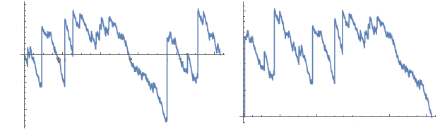
Since almost surely, we get that almost surely. Moreover, is clearly càdlàg and Markov with stationary and independent increments, as has these properties, and therefore is a Lévy process. The following proposition computes its Laplace exponent and its characteristic exponent.
Proposition 5.2.
Fix , . Then
- (i)
The Laplace exponent of has the form where is the only real solution of the equation
(11) - (ii)
The characteristic exponent of has the form , where is the only solution with nonnegative real part of the equation
(12)
Remark that by Proposition 5.2 (ii), as , , and therefore . Hence, as , and in particular
| (13) |
Thus, verifies the assumption of Theorem 5.1, and therefore admits a density. In addition, one can easily check that is spectrally positive. This allows us to define the excursion and the lamination .
Proof of Proposition 5.2.
Let us first prove (i). Since is a stopping time according to the canonical filtration associated to and is almost surely finite, for any , by Doob’s stopping time theorem,
Now remark that for , . Therefore , which can be rewritten .
Since is a bijection from to itself, we get that for all ,
5.2 A new family of random trees
The key idea of the proof of Theorem 1.3 is to introduce a new sequence of conditioned random trees , such that the sequence converges in distribution towards both and (Theorem 5.3). These trees are Galton-Watson trees conditioned by their number of vertices, whose offspring distribution varies with .
Let be a critical distribution in the domain of attraction of an -stable law, and a sequence verifying (4). We recall that denotes a -GW tree, and that denotes a -GW tree conditioned to have vertices. For large enough so that , define
and let be the law whose generating function verifies
| (14) |
where is the generating function of (that is, for , ). Remark, by taking in (14), that is also critical for all . We let be a nonconditioned GW tree with offspring distribution , and be the tree conditioned to have vertices, for . Remark that, by (14), for any , any , as soon as . Note also that (14) appears in [13, Proposition (i)] (taking in this Proposition ), where Bertoin studies a similar model of random trees coding rare mutations in a population.
Theorem 5.3.
The following two convergences hold in distribution, as :
- (i)
- (ii)
We prove the two parts of Theorem 5.3 separately.
5.3 Proof of Theorem 5.3 (i)
In order to prove Theorem 5.3 (i), we start by seeing as a reduced version of a -GW tree. To this aim, let us define the notion of vertex-marking process on a tree. Let be a plane tree, and be the set of its vertices. A vertex-marking process on is a function such that . We say that a vertex is marked if . To a vertex-marking process on a plane tree , we associate the reduced tree defined the following way:
- •
the set of vertices of is the set of marked vertices of : .
- •
we erase all the edges of the initial tree .
- •
we put a new edge between two vertices of if one is the nearest marked ancestor of the other in .
(see an example on Fig. 16).
A natural vertex-marking process on a tree consists in marking the root, and marking each other vertex independently with probability . We denote this process by . Notice that the associated reduced tree is essentially a conditioned version of the tree of alleles of Bertoin [13], where one forgets about the labels of the vertices.
The proof is based on the study of the reduced tree, and consists in proving that the lamination associated to this tree is roughly the sublamination of built by drawing only chords that correspond to marked vertices. For this, we mostly use concentration inequalities on binomial variables. First, remark that the (nonconditioned) GW tree is distributed as . Therefore we can focus on the lamination , where is a -GW tree.
The first technical lemma concerns the size of , conditionally to the event that . Its proof is postponed to the end of the paragraph. Let us introduce a notation: a sequence being given, we say that if there exists , such that for all .
Lemma 5.4.
As ,
Proof.
In order to prove this lemma, observe that for a tree , conditionally to , we have for ,
by Chernoff inequality, where . Observe that, for any , . This allows us to write:
On the other hand, remark that
By the local limit theorem 4.7, decays at most polynomially in . At the same time, decays at most polynomially as well.
On the other hand, and is bounded by for large enough and . The result follows. ∎
This lemma allows us to restrict ourselves to the study of a tree with roughly vertices, exactly of which are marked. In what follows, we fix and place ourselves under the two conditions: and . Indeed, by Lemma 5.4 and Theorem 3.2, proving the convergence of Theorem 5.3 (i) under these conditions in enough to get it in whole generality (again, this convergence has to be understood as: under these conditions, the lamination admits a limit, which converges to as ). We denote by the set of trees verifying these two conditions.
For a given finite tree , we denote by the set of marked vertices of . In what follows, for , denotes the set of vertices of such that (where we recall that is the subtree of rooted in ). Remark that is always nonempty since it contains at least the root. We now define three events on a finite tree with marked vertices (including the root).
: there exists such that and that the number of marked vertices in is . In other words, this is the event that there exists a small subtree which contains a large number of marked vertices.
: . The number of marked vertices whose subtree contains more than vertices is equal to .
Notice that, under the event , one can separate into components the following way: taking the first and last times that each element of is visited by the contour function of , we get times between and , which we order increasingly. The components correspond to the vertices visited for the first time by the contour exploration between two consecutive of these times. Since the root is in , and belong to this set of times and these components form a partition of . Denote the components by , and their respective sizes by . Finally, denote by the number of marked vertices in .
: holds and there exists such that and such that, in addition, . We will prove that, for all , with high probability, this even does not occur. In other words, the number of marked vertices in each of these components is very concentrated around its mean.
We get convergences of the probabilities of these three events, uniformly on , as . In the following theorem, the probability has to be understood in the sense that the tree is fixed, and the marked vertices are random.
Proposition 5.5.
- (i)
.
- (ii)
For any , where . In particular, these values sum to .
- (iii)
For any , .
Let us immediately see how it implies Theorem 5.3 (i)
Proof of Theorem 5.3 (i) using Proposition 5.5.
We will prove that is close in distribution to under the assumptions and , which will straightforwardly imply Theorem 5.3 (i) by Theorem 3.3. To this end, we will prove that large chords have almost the same location in both laminations.
For , define a uniform variable on the edge from to its parent, so that are independent. Then, remark that, on one hand, the chords corresponding to and are at distance at most in . On the other hand, by Proposition 5.5 (ii), the set is asymptotically distributed as a Poisson point process of intensity , on the set of edges of whose endpoints are in (conditionally given that no two points of are in the same edge, which happens with high probability).
Proposition 5.5 (i) ensures that large chords (namely, chords that have length ) in are necessarily coded by points of .
Finally, by Proposition 5.5,(iii), each chord in coded by a vertex of is asymptotically close to the chord corresponding to in , which concludes the proof. ∎
Now we prove Proposition 5.5.
Proof of Proposition 5.5.
The proofs of these three statements rely on estimates of binomial tails. Let us start by proving (ii). For ,
where and . We now use the following key fact: for any tree , any , let be the number of vertices of such that . Then
| (15) |
Indeed, being fixed, there are at most such vertices with height exactly . The result follows by summing over all . In particular, uniformly in , . Hence, as , and
where is a Poisson variable of parameter .
In order to prove (i), we use a similar method. Take and such that . Then the probability that there are marked vertices in is
where and . By the local limit theorem 4.7, there exists a constant depending only on such that, uniformly in , . Hence, the probability that there are more that vertices in satisfies . By Bienaymé-Tchebytchev inequality, for large enough,
Since , we obtain:
Now observe that, by (15), the number of vertices in (marked or not) such that is . Hence, with high probability, the number of such vertices that are marked is . Distinguishing marked vertices such that and marked vertices such that , we get that there exists a constant such that
using the fact that the number of marked vertices in is exactly . This quantity tends to , which provides the result.
Finally, we sketch the idea of the proof of (iii). Remark that are distributed as binomials of parameters , conditionally to their sum being equal to . The only thing that we need to prove is that, as grows, for any , for any , for any subset of points of independent of the vertex-marking process, the number of marked vertices among these points is concentrated enough around its mean. More precisely, since follows a binomial distribution of parameters , we only need to prove that
where . As in the proof of Lemma 5.4, this is a direct application of Chernoff inequality. The result follows. ∎
5.4 Proof of Theorem 5.3 (ii)
In order to prove this part of the theorem, we need to introduce an other way of coding a finite tree, called the Lukasiewicz path of the tree (see Fig. 17 for an example). Let be a plane tree with vertices. Its Lukasiewicz path is constructed as follows: and, for , . In particular, . We define it on the whole interval by taking its linear interpolation.
Recall that we defined in Section 1.1 a lamination associated to a tree through its contour function. Here, we shall need another lamination, which is discrete, defined through its Lukasiewicz path. Specifically, fix a plane tree with vertices. For every , set , and set
(see Fig. 17 for an example).
The following result shows that the laminations and are close, provided that is a large tree with rather small height.
Lemma 5.6.
Let be such that . Then
Proof.
Let be a tree with vertices and height . Let , and recall that denotes the -th vertex of in the lexicographical order. Let be the size of the subtree rooted at . Then, corresponds to a chord between and in . In , codes a chord between and , while points in the edge between and its parent code (infinitely many) chords at distance to this first one. The result follows since, by assumption, uniformly for all , . ∎
Recall that is a Galton-Watson tree with offspring distribution , conditioned on having vertices. The main tool to establish Theorem 5.3 (ii) is the fact that the Lukasiewicz path of is distributed as a conditioned random walk (see [41, Section 1.2]). More precisely, let be the integer-valued random walk started from with i.i.d. jumps, whose jump distribution is given by for . We extend it on by linear interpolation. Then, conditioned on the event is distributed as the Lukasiewicz path of the tree . In order to obtain a limit theorem for , we rely on the following local limit theorem.
Theorem 5.7.
Fix . The following convergence holds as :
where is the density of .
The proof of this result is postponed to Section 5.5; let us first explain how it entails Theorem 5.3 (ii).
Proof of Theorem 5.3 (ii) from Theorem 5.7.
The first step is to show that the convergence
holds in distribution. To this end, we follow the classical path, which consists in first showing a convergence under a “bridge” condition by combining an unconditioned convergence with absolute continuity and time-reversal, and then using the Vervaat transformation. To do it, we start by proving an unconditioned convergence, namely
| (16) |
By [34, Theorem 16.14], to prove (16), it is enough to check that the one-dimensional convergence holds for , which is an immediate consequence of Theorem 5.7.
Next, we prove the "bridge" version of this theorem, first up to time . Let be a continuous bounded function. Then, setting , by absolute continuity, we have
By combining Theorem 5.7 and (16), this quantity converges to as . By (10), this is equal to . In order to obtain the convergence up to time , it is enough to show tightness on . Observe that we already know that, conditionally given , the sequence is tight on . In order to prove that it is tight on , we prove that, for , the process is tight on . For this, just remark that by time-reversal,
which is tight conditionally given by the previous observation.
In order to deduce the convergence of the excursions from the convergence of the bridge versions of the processes, we make use of the Vervaat transform, following Definition Definition. Note that the minimum of is almost surely unique. Indeed, it is true for the unconditioned version and transfers to the bridge by the absolute continuity relation (10). Therefore, the Verwaat transform is continuous at , and by applying it to the bridge convergence this completes the first step.
To prove that the convergence of the rescaled Lukasiewicz paths of to implies the convergence of to , first note that a straightforward adaptation of [38, Proposition 3.5] shows that converges in distribution to as . To conclude the proof, in view of Lemma 5.6, it remains to check that with high probability. Let us prove that in fact, with high probability, . To this end, remark that the height of a vertex in is the number of marked vertices in the ancestral line of the corresponding vertex in . Now let be a marked vertex and be its height. Then, copying the proof of Proposition 5.5 (i), there exists a constant such that, if and , we have by Chernoff inequality:
for large enough, where is the number of marked vertices in the ancestral line of in (the exponents used here are not optimal but are sufficient to get our result). Here we have used the fact that there exists a constant such that for all large enough. Hence, by a union bound over all vertices in the tree, with high probability no marked vertex has more than marked vertices in its ancestral line, which concludes the proof. ∎
5.5 Proof of the local estimate
In this section, we establish Theorem 5.7. For and , the following quantity will play an important role:
The proof relies on the following estimates. Recall that denotes the characteristic exponent of .
Lemma 5.8.
The following assertions are satisfied:
- (i)
The convergence holds as , uniformly for .
- (ii)
Let be a compact subset of which does not contain . The convergence holds as , uniformly for .
- (iii)
For , set
Then, for every , there exists such that, for large enough, for every such that , we have and .
Proof of Theorem 5.7 using Lemma 5.8.
Fix . In the whole proof, for convenience, we will write instead of . We let be the characteristic function of and be its density (which we recall exists by Theorem 5.1). Fix . The goal is to prove that, for large enough, uniformly in such that , uniformly in ,
| (17) |
For , , we set . First, by Fourier inversion, we have for all : . Hence, for such that is an integer, we can write
Therefore, for any , we can write
where
We now bound these four quantities, for certain well chosen.
Bounding . Straightforwardly, since and are bounded by on , for all .
Bounding . Since, by definition, , Lemma 5.8 (ii) entails that, at fixed, as , uniformly in .
Bounding . We have already seen that as . Thus, decays exponentially fast as , and as (remark that does not depend on ). Hence, for large enough, .
Bounding . The main challenge is in fact to bound . To this aim, we deeply use Lemma 5.8 (ii) and (iii). For , we have
| (18) | |||||
We keep the notation of Lemma 5.8 (iii) and assume that is large enough, so that for every large enough and we have and
| (19) |
Note that for all , that for , and that for , . Therefore, by (19), uniformly for , is bounded away from , and therefore for some constant . Recall indeed that for all . Then, by (18),
On the other hand, uniformly for , by Lemma 5.8 (ii). Hence, for large enough and ,
where we have used the Potter bounds 3.1 and the fact that . Hence, (19) gives:
which is less than for some absolute constant , using the fact that for . We finally get for large enough, for every large enough and
| (20) |
Thus, for large enoug, for any large enough and any , . This completes the proof. ∎
We now prove separately the three parts of Lemma 5.8.
Proof of Lemma 5.8 (i).
It is enough to show that as . Let us denote, for , . By (14), . In particular, . Since is continuous on (and hence uniformly continuous), we just have to prove that is the only fixed point of . For this, we use the fact that is critical, which implies that is negative on and is decreasing. Since , on which concludes the proof. ∎
The proofs of Lemma 5.8 (ii) and (iii) use the following estimate.
Lemma 5.9.
As , uniformly for ,
where the holds when , uniformly in , and where is the slowly varying function defined in (3).
Proof.
Our main object of interest is the generating function of . It is notably known (see [26, , Theorem ]) that has the following Taylor expansion at , on the real axis:
| (21) |
where is the slowly varying function given by (3).
Now, observe that, if , . To see this, remark that by (14),
which is possible only if by the case of equality in the triangular inequality (using the fact that ). This implies that, if , and we can apply Theorem 1.4 to (14). To simplify notation, set . By Lemma 5.8 (i), uniformly in , and when we can write:
Hence, by Theorem 1.4 and (21),
where we have set to simplify notation. Therefore:
| (22) |
By Lemma 5.8 (i), - and therefore - both converge to uniformly for . Hence (22) immediately implies that , and thus that . This allows us to reduce (22) to
Remember that by definition . Then
which boils down, by (4), to
uniformly in . This completes the proof. ∎
Proof of Lemma 5.8 (ii).
We show this convergence by analyzing the implicit equation (14). Let be a compact subset of which does not contain . Lemma 5.9 implies that, uniformly for ,
| (23) |
Now remark that, by the Potter bounds 3.1, for large enough,
Hence, by (23), there exists such that, for large enough and for all (using the fact that ), . This implies that, uniformly for , as , and that (23) reduces to . Remember that for all , , . Therefore converges to the unique solution of (12) with nonnegative real part, which is the characteristic exponent of . ∎
Proof of Lemma 5.8 (iii).
From Lemma 5.9, we get
| (24) |
First, for , we have , which tends to as . Second, by the Potter bounds 3.1, for large enough. These two observations, combined with (24), readily entail that for fixed , we can find such that uniformly for , .
Now fix and such that, for all , . In particular, for , and we get from (24):
for large enough, using the fact that by the Potter bounds. Therefore, . Now remark that is bounded away from , uniformly in . Then is necessarily close to , which readily entails that where as . This completes the proof. ∎
5.6 Study of the solutions of the implicit equation (12)
We finish this section by proving that (12) has only one solution with nonnegative real part and that this real part is positive for ; this will imply that this solution is by Proposition 5.2 (ii). Fix , and denote by the function
Therefore, (12) can be rewritten , and we are interested in the solutions in , at and fixed, of the equation
| (25) |
Note that we also define for although we are only interested in the case , as this allows to use the implicit function theorem at .
Theorem 5.10.
For any and , (25) has exactly one solution with nonnegative real part, and this real part is positive.
Proof of Theorem 5.10.
We first prove that (25) has a unique such solution for large enough. Then we use the local continuity in and of the solutions of (25) to extend it to all . First, remark that, at fixed, is on , and its derivative with respect to is
| (26) |
which is always nonzero when is a solution of (25).
In the case , (25) has two solutions that are . As , these solutions are equivalent to . Therefore, we can take large such that (25) has exactly one solution with positive real part for and . Assume that the real part of a solution of (25) is never . Then, by (26), we can use the implicit function theorem around any solution of (25). This entails that for any there exists exactly one solution of that has positive real part. Using again the implicit function theorem at fixed by letting vary from to any positive value of , we get Theorem 5.10.
Remark.
One can prove that, for and large enough, (25) has a second solution which has negative real part. This "negative branch" ultimately vanishes at some , and the corresponding solutions of (25) converge to the negative real line. The discontinuity of the branch shall therefore be related to the fact that the function is not defined on this line.
6 Generating functions of stable offspring distributions
This section is devoted to the proof of Theorem 1.4. We fix a critical offspring distribution (that is, a probability distribution on the nonnegative integers with mean ), and we assume that there exists and a slowly varying function such that
where denotes the generating function of . This is equivalent to saying that is in the domain of attraction of an -stable law. We define , the slowly varying function such that
| (27) |
By e.g. [26, , Theorem ] and [16, Lemma ], if is a random variable of law , then the following statement holds:
| (28) |
where is the function appearing in (27). Note that the "" term is negligible except when has finite variance, in which case .
Let us first introduce some notation. For , we set . The main tool in the proof of Theorem 1.4 is the following estimate.
Proposition 6.1.
As , with ,
where if and otherwise.
Note that there is an extra term "" when . Before proving this result, let us explain how Theorem 1.4 then readily follows.
Proof of Theorem 1.4.
We first show that
| (29) |
To this end, observe that for such that ,
| (30) |
Indeed,
which is equal to . The estimate (29) then follows from Proposition 6.1.
Now, remark that, for such that , , where is defined as in Definition Definition. Hence, we can apply (29) to . Then, as while , by expanding around and using the fact that a slowly varying function varies more slowly than any polynomial, we get that is equal to
and this completes the proof. ∎
The statement of Proposition 6.1 is slightly different whether or , and therefore we need two different proofs. The reason comes from the following useful estimate (see [26, Corollary and ]):
| (31) |
where is a slowly varying function such that .
6.1 Proof of Proposition 6.1 for
We start with the case , which is easier. In what follows, we set such that, for all , ,
| (32) |
The existence of such a is guaranteed by (28) as soon as . The proof of Proposition 6.1 is based on the following lemma:
Lemma 6.2.
The following assertions hold.
- (i)
As , .
- (ii)
Fix and verifying (32). Then, for large enough and such that , we have
Proof.
For the first assertion simply write, for ,
For (ii), observe that for such that , we have . Hence, when , one has:
Hence, by (i), for large enough and , we have , which is at most . This completes the proof.
∎
Proof of Proposition 6.1 for .
We assume that . Fix . For with , let . Therefore, Lemma 6.2 (ii) holds with for small enough and we get
where we have used Lemma 6.2 (ii) and the fact that as (see [15, Proposition ]). Since , it follows that for small enough,
| (33) |
But by Lemma 6.2 (i), as . The desired result is obtained by taking , using the facts that as , and that when .
∎
6.2 Proof of Proposition 6.1 for
We now fix . In the sequel, we fix such that for every :
| (34) |
The proof is based on two technical estimates.
Lemma 6.3.
The following assertions hold:
- (i)
uniformly for with negative real part,
- (ii)
for any fixed , we have
Proof.
For the first assertion, we use tools from complex analysis. For , define the path as in Fig. 18, as the union of two straight lines and two arcs and . Since is holomorphic on , the value of its integral on this path is .
By (34), for , uniformly for with negative real part,
and
On the other hand, as and , . This shows the first equality in (i). The second one is a simple computation.
For (ii), the idea is to write
for some to be fixed later, and to estimate the three terms. Let us fix .
Third term. By the Potter bounds, we may fix such that, for any , for and , we have . This implies that, for ,
which is less than for large enough (independent of ). In what follows, we take such that this holds.
First term. By the Potter bounds, there exists such that, for small enough and , we have . Furthermore, by (34), for small enough,
which is less than for small enough (independent of ). In what follows, we take such that this holds.
Second term. Since is slowly varying, uniformly in , as . Therefore, for any , for small enough (depending on ),
where the last inequality follows from a change of variables. We conclude that for small enough (depending on and ),
By putting together the three previous estimates, we get
as . To conclude the proof, remark that by change of variables,
which converges towards as , by (i).
∎
Proof of Proposition 6.1 in the case .
Let us assume that and recall that the goal is to estimate . The idea is to write
for certain well chosen and to estimate separately these two terms. Using (31), we shall show that as , the first term is , while the second one is asymptotic to . Again, some care is needed as we are dealing with complex-valued quantities.
First term.
First of all, by definition, for any , . Therefore, setting and using (34),
for small enough. As a consequence, as .
Second term.
Fix . By the estimate (31), as , uniformly for , . This allows us to write for any , for small enough (depending on ):
In particular, mimicking the proof of Lemma 6.3 (ii), we bound the right-hand term and get, for small enough,
The desired result then follows from the estimate of Lemma 6.3 (ii).
∎
References
- [1] R. Abraham and J.-F. Delmas. Fragmentation associated with Lévy processes using snake. Probability Theory and Related Fields, 141(1-2):113–154, 2008.
- [2] R. Abraham and J.-F. Delmas. Local limits of conditioned Galton-Watson trees I: the infinite spine case. 2013.
- [3] R. Abraham, J.-F. Delmas, and G. Voisin. Pruning a Lévy continuum random tree. Electronic journal of probability, 15:1429–1473, 2010.
- [4] R. Abraham and L. Serlet. Poisson snake and fragmentation. Electronic Journal of Probability, 7, 2002.
- [5] D. Aldous. Triangulating the circle, at random. The American Mathematical Monthly, 101:223–233, 1994.
- [6] D. Aldous. Brownian excursions, critical random graphs and the multiplicative coalescent. The Annals of Probability, pages 812–854, 1997.
- [7] D. Aldous and V. Limic. The entrance boundary of the multiplicative coalescent. Electron. J. Probab, 3(3):59, 1998.
- [8] D. Aldous and J. Pitman. The standard additive coalescent. Annals of Probability, pages 1703–1726, 1998.
- [9] S. Athreya, W. Löhr, A. Winter, et al. Invariance principle for variable speed random walks on trees. The Annals of Probability, 45(2):625–667, 2017.
- [10] J. Bertoin. A fragmentation process connected to Brownian motion. Probability Theory and Related Fields, 117(2):289–301, 2000.
- [11] J. Bertoin. Random Fragmentation and Coagulation Processes. Cambridge Studies in Advanced Mathematics. Cambridge University Press, 2006.
- [12] J. Bertoin. Asymptotic regimes for the partition into colonies of a branching process with emigration. The Annals of Applied Probability, 20(6):1967–1988, 2010.
- [13] J. Bertoin. A limit theorem for trees of alleles in branching processes with rare neutral mutations. Stochastic Process. Appl., 120(5):678–697, 2010.
- [14] J. Bettinelli. Convergence of uniform noncrossing partitions toward the Brownian triangulation. arXiv preprint arXiv:1711.04872, 2017.
- [15] N. H. Bingham, C. M. Goldie, and J. L. Teugels. Regular variation, volume 27. Cambridge university press, 1989.
- [16] J. E. Björnberg and S. Ö. Stefánsson. Random walk on random infinite looptrees. Journal of Statistical Physics, 158(6):1234–1261, 2015.
- [17] F. Bonahon. Geodesic laminations on surfaces. In Laminations and foliations in dynamics, geometry and topology (Stony Brook, NY, 1998), volume 269 of Contemp. Math., pages 1–37. Amer. Math. Soc., Providence, RI, 2001.
- [18] P. Chassaing and G. Louchard. Phase transition for parking blocks, Brownian excursion and coalescence. Random Structures & Algorithms, 21(1):76–119, 2002.
- [19] L. Chaumont and G. U. Bravo. Markovian bridges: weak continuity and pathwise constructions. The Annals of Probability, 39(2):609–647, 2011.
- [20] N. Curien and I. Kortchemski. Random non-crossing plane configurations: A conditioned Galton-Watson tree approach. Random Structures & Algorithms, 45(2):236–260, 2014.
- [21] N. Curien and J.-F. Le Gall. Random recursive triangulations of the disk via fragmentation theory. The Annals of Probability, 39(6):2224–2270, 2011.
- [22] N. Curien and W. Werner. The Markovian hyperbolic triangulation. Journal of the European Mathematical Society, 15(4):1309–1341, 2013.
- [23] J. Dénes. The representation of a permutation as the product of a minimal number of transpositions and its connection with the theory of graphs. Publ. Math. Inst. Hungar. Acad. Sci, 4:63–70, 1959.
- [24] T. Duquesne et al. An elementary proof of Hawkes’s conjecture on Galton-Watson trees. Electronic Communications in Probability, 14:151–164, 2009.
- [25] T. Duquesne and J.-F. Le Gall. Random Trees, Lévy Processes and Spatial Branching Processes. 2002.
- [26] W. Feller. An introduction to probability theory and its applications, volume 2. John Wiley & Sons, 2008.
- [27] V. Féray and I. Kortchemski. The geometry of random minimal factorizations of a long cycle. arXiv preprint arXiv:1712.06542, 2017.
- [28] V. Féray and I. Kortchemski. Trajectories in random minimal transposition factorizations. arXiv preprint arXiv:1810.07586, 2018.
- [29] P. Flajolet and R. Sedgewick. Analytic combinatorics. Cambridge University Press, Cambridge, 2009.
- [30] I. Goulden and A. Yong. Tree-like properties of cycle factorizations. Journal of Combinatorial Theory, Series A, 98(1):106–117, 2002.
- [31] I. A. Ibragimov and Y. V. Linnik. Independent and stationary sequences of random variables. Wolters-Noordhoff Publishing, Groningen, 1971. With a supplementary chapter by I. A. Ibragimov and V. V. Petrov, Translation from the Russian edited by J. F. C. Kingman.
- [32] J. Jacod and A. Shiryaev. Limit theorems for stochastic processes, volume 288. Springer Science & Business Media, 2013.
- [33] S. Janson. Simply generated trees, conditioned Galton–Watson trees, random allocations and condensation. Probability Surveys, 9:103–252, 2012.
- [34] O. Kallenberg. Foundations of Modern Probability. 2002.
- [35] O. Kallenberg et al. Splitting at backward times in regenerative sets. The Annals of Probability, 9(5):781–799, 1981.
- [36] H. Kesten. Subdiffusive behavior of random walk on a random cluster. Ann. Inst. H. Poincaré Probab. Statist., 22(4):425–487, 1986.
- [37] J. F. C. Kingman. The coalescent. Stochastic processes and their applications, 13(3):235–248, 1982.
- [38] I. Kortchemski. Random stable laminations of the disk. The Annals of Probability, 42(2):725–759, 2014.
- [39] I. Kortchemski and C. Marzouk. Triangulating stable laminations. Electronic Journal of Probability, 21, 2016.
- [40] I. Kortchemski and C. Marzouk. Simply generated non-crossing partitions. Combinatorics, Probability and Computing, 26(4):560–592, 2017.
- [41] J.-F. Le Gall et al. Random trees and applications. Probability surveys, 2:245–311, 2005.
- [42] J.-F. Le Gall, Y. Le Jan, et al. Branching processes in Lévy processes: the exploration process. The Annals of Probability, 26(1):213–252, 1998.
- [43] J.-F. Le Gall and F. Paulin. Scaling limits of bipartite planar maps are homeomorphic to the 2-sphere. Geometric and Functional Analysis, 18(3):893–918, 2008.
- [44] J.-F. Marckert and M. Wang. A new combinatorial representation of the additive coalescent. Random Structures Algorithms, 54(2):340–370, 2019.
- [45] G. Miermont. Ordered additive coalescent and fragmentations associated to Lévy processes with no positive jumps. Electronic Journal of Probability, 6, 2001.
- [46] G. Miermont. Self-similar fragmentations derived from the stable tree I. Probability Theory and Related Fields, 127(3):423–454, 2003.
- [47] G. Miermont. Self-similar fragmentations derived from the stable tree II: splitting at nodes. Probability theory and related fields, 131(3):341–375, 2005.
- [48] P. Moszkowski. A solution to a problem of Dénes: a bijection between trees and factorizations of cyclic permutations. European Journal of Combinatorics, 10(1):13–16, 1989.
- [49] J. Neveu. Arbres et processus de Galton-Watson. Ann. Inst. H. Poincaré Probab. Statist., 22(2):199–207, 1986.
- [50] J. Pitman. Combinatorial stochastic processes. Technical report, Technical Report 621, Dept. Statistics, UC Berkeley, 2002. Lecture notes for St. Flour course, 2002.
- [51] Q. Shi. On the number of large triangles in the Brownian triangulation and fragmentation processes. Stochastic Process. Appl., 125(11):4321–4350, 2015.
- [52] R. Slack. A branching process with mean one and possibly infinite variance. Probability Theory and Related Fields, 9(2):139–145, 1968.
- [53] D. Tokarev. Growth of integral transforms and extinction in critical galton-watson processes. Journal of Applied Probability, 45(2):472–480, 2008.
- [54] G. Voisin. Dislocation measure of the fragmentation of a general Lévy tree. ESAIM: Probability and Statistics, 15:372–389, 2011.