Gromov-Wasserstein Averaging in a Riemannian Framework

A metric measure (mm) space is a compact metric space endowed with a Borel probability measure. Gromov-Wasserstein (GW) distance was first introduced as a metric on the space of all (isomorphism classes of) mm spaces. Theoretical aspects of the GW distance were explored in dgh-sm; dghlp; sturm2012space. The work in dgh-sm; dghlp was already focused on applications to object matching, while sturm2012space explored the Riemannian-like structures induced by GW distance.

In recent years, GW distance has garnered interest in data science communities as a way to compare unlabeled datasets, or datasets containing samples from different ambient spaces. For example, GW distance has been used to explore a variety of network datasets hendrikson2016using, as a metric alignment layer in deep learning algorithms for object classification ezuz2017gwcnn, to align word embedding spaces for translation applications alvarez2018gromov, for several tasks in analysis of large graphs and networks xu2019gromov; xu2019scalable, and has been incorporated into generative models across incomparable spaces bunne2019learning. Several specialized variants of GW distance have also been recently introduced memoli2018gromov; titouan2019optimal; titouan2019sliced.

The problem of computing GW distance was studied from the algorithmic viewpoint in pcs16, where a projected gradient descent algorithm was introduced. The main focus was on using GW distance to compute a Fréchet mean with prescribed size of distance (or kernel) matrices. The main idea of the present paper is to recast the work in pcs16 using the theoretical Riemannian framework of sturm2012space together with statistical algorithms on Riemannian manifolds pennec. By using this viewpoint, we are able to generalize the work of pcs16 to a gradient flow that theoretically prescribes the required size for a Fréchet mean, while providing a flexible general framework for machine learning tasks on network-valued datasets. This includes the case of asymmetric networks.

An approach similar to that of the present paper to studying statistics on the space of graphs via Riemannian geometry was initiated in jain2009structure; jain2012learning. Recently, these ideas were applied to formulate a theory of statistical shape analysis of embedded graphs in guo2019quotient. These works perform analysis on graph space by aligning graph nodes over permutations or “hard matchings”, whereas our approach aligns networks via measure couplings or “soft matchings”. The differences between these theories are interesting, and we expect that the correct formalism to use is highly dependent on the particular application.

Our specific contributions are as follows. We first provide the gradient of the GW functional on asymmetric networks. This complements a similar result for symmetric matrices in pcs16. On the metric geometry side, we provide a concrete exposition of the tangent space structure on this space of asymmetric networks and of the construction of geodesics in the space of networks. This includes the, to our knowledge, first computationally feasible algorithm to produce Sturm geodesics. We explicitly formulate the iterative Fréchet mean algorithm of Pennec as gradient descent of the Fréchet functional on the space of networks. The tangent structure provides a framework for vectorizing collections of networks in order to apply standard ML algorithms. We exemplify this by performing averaging and principal component analysis on a database of planar shapes. Our methods can also be used for network compression, and we illustrate this on a toy example of an asymmetric stochastic blockmodel network.

A measure network is a triple $(X,\omega_{X},\mu_{X})$ where $X$ is a Polish space (i.e. separable, completely metrizable), $\mu_{X}$ is a fully supported Borel probability measure, and $\omega_{X}:X\times X\rightarrow\mathbb{R}$ is a square integrable function. The collection of all networks is denoted $\mathcal{N}$. When no confusion will arise, we abuse notation and denote the triple $(X,\omega_{X},\mu_{X})$ by $X$.

The notion of a measure network is quite general and includes several types of spaces which arise in applications. A graph can be represented as a measure network: $X$ is set of $n$ nodes, while $\omega_{X}$ provides relational information and could be represented by a weighted adjacency matrix, a graph Laplacian, or a matrix of graph distances (for connected graphs or strongly connected digraphs)—see Example 2. The probability measure $\mu_{X}$ can be taken to be uniform, or could more generally give higher weight to nodes deemed more important by a particular application. The notion of a measure network is also a strict generalization of that of a metric measure space, as defined in the previous section. For a finite metric measure space, $\omega_{X}$ can be represented as by its distance matrix. Our definition also includes infinite spaces—this is necessary for certain theoretical completeness results to hold, but the reader more interested in applications can safely restrict their attention to finite spaces.

A coupling between two probability measures $\mu_{X}$ and $\mu_{Y}$ supported on Polish spaces $X$ and $Y$ is a probability measure on $X\times Y$ with marginals $\mu_{X}$ and $\mu_{Y}$. Stated differently, $\mu(A\times Y)=\mu_{X}(A)$ for all $A\in\operatorname{Borel}(X)$ and $\mu(X\times B)=\mu_{Y}(B)$ for all $B\in\operatorname{Borel}(Y)$. The collection of all such couplings is denoted $\mathscr{C}(\mu_{X},\mu_{Y})$.

Intuitively, for finite measure networks $X$ and $Y$ and a coupling $\mu$, the value of the coupling $\mu(x_{i},y_{j})$ can be understood as an assignment of a certain proportion of the mass $\mu_{X}(x_{i})$ to the point $y_{j}$. In the graph setting, this is a “soft matching” of the nodes of $X$ and $Y$. One then wishes to find a soft matching which reflects similarity of $X$ and $Y$ as well as possible. This is formalized by the notion of distortion, defined below.

Given two networks $(X,\omega_{X},\mu_{X})$ and $(Y,\omega_{Y},\mu_{Y})$ in $\mathcal{N}$, one defines the distortion functional to be the map

More explicitly, $\operatorname{dis}(\mu)$ is the quantity

where the integral is taken over the space $X\times Y\times X\times Y$. The Gromov-Wasserstein distance between networks $(X,\omega_{X},\mu_{X})$ and $(Y,\omega_{Y},\mu_{Y})$ is then defined by

One may similarly define the $p$-GW distance by taking the $L^{p}$ norm, but the constructions in this paper rely on the special structure of the $L^{2}$ case.

The following lemma shows that the infimum in the definition above is always achieved. Minimizers of $\operatorname{dis}$ are referred to as optimal couplings. The proof follows directly from (sturm2012space, Lemma 1.2).

In the finite setting, the notation of pcs16 admits some useful insights into this minimization problem. We present this notation now. Let $L:\mathbb{R}\times\mathbb{R}\rightarrow\mathbb{R}$ be a loss function. In our case, this will always be defined as $L(a,b):=\left|a-b\right|^{2}$. Next we switch to matrix notation: given a finite space $X=\{x_{1},x_{2},\ldots,x_{n}\}$, we write $X_{ik}$ to denote $\omega_{X}(x_{i},x_{k})$ for $1\leq i,k\leq n$. Suppose $Y$ is another finite space of size $m$. The collection of couplings $\mathscr{C}(\mu_{X},\mu_{Y})$ then consists of $n\times m$ matrices $C=(C_{ij})_{ij}$ such that

Then one defines the 4-way tensor $\mathcal{L}(X,Y):=\left(L(X_{ik},Y_{jl})\right)_{ijkl}$. Given a 4-way tensor $\mathcal{L}$ and a matrix $\left(C_{ij}\right)_{ij}$, one defines the tensor-matrix multiplication

Next, given two real-valued matrices $A$ and $B$ of the same dimensions, one writes $\langle A,B\rangle$ to denote the Frobenius inner product $\sum_{ij}A_{ij}B_{ij}$. As observed in pcs16, the GW distance between two finite networks $X$ and $Y$ can be written as:

For the reader’s convenience, we verify that the dimensions are consistent. If $X$ is an $n$-point space and $Y$ is an $m$-point space. Then $C$ is an $n\times m$ coupling matrix, $\mathcal{L}(X,Y)$ is an $n^{2}\times m^{2}$ tensor, and the product $\mathcal{L}(X,Y)\otimes C$ is an $n\times m$ matrix. An alternative matrix formulation s16 of the term inside the $\min$ is the following:

Here $.^{\wedge 2}$ denotes the elementwise square. While this formulation is well-known, we provide details in the appendix for the reader’s convenience.

The space $(\mathcal{N},d_{\mathcal{N}})$ is a pseudometric space. Networks $(X,\omega_{X},\mu_{X})$ and $(Y,\omega_{Y},\mu_{Y})$ satisfy $d_{\mathcal{N}}(X,Y)=0$ if and only if there exists a Borel probability space $(Z,\mu_{Z})$ with maps $\pi_{X}:Z\rightarrow X$ and $\pi_{Y}:Z\rightarrow Y$ such that the pushforward measures satisfy $(\pi_{X})_{\#}\mu_{Z}=\mu_{X}$, $(\pi_{Y})_{\#}\mu_{Z}=\mu_{Y}$, and the pullbacks $(\pi_{X})^{*}\omega_{X}$, $(\pi_{Y})^{*}\omega_{Y}$ satisfy $\|(\pi_{X})^{*}\omega_{X}-(\pi_{Y})^{*}\omega_{Y}\|_{\infty}=0$, where $(\pi_{X})^{\ast}\omega_{X}(z,z^{\prime}):=\omega_{X}(\pi_{X}(z),\pi_{X}(z^{\prime}))$. In this case, $X$ and $Y$ are said to be weakly isomorphic and write $X\cong^{w}Y$. The space $Z$ is referred to as a common expansion of $X$ and $Y$. We write $[X]=[X,\omega_{X},\mu_{X}]$ to denote the weak isomorphism class of $X=(X,\omega_{X},\mu_{X})$ in $\mathcal{N}$. The collection of equivalence of classes of networks will be denoted $[\mathcal{N}]$. See also gwnets for more details on weak isomorphism.

In the case of finite networks, weak isomorphism is especially useful as it allows one to convert transport plans (i.e., couplings between the networks’ measures) to transport maps (i.e., measure-preserving maps between networks). This observation plays a key role in both our theory and algorithms. We present this construction next.

It was implicitly observed in Section 2.1 that for finite measure networks $X$ of size $n$ an $Y$ of size $m$, the squared distortion of a coupling matrix $C\in\mathscr{C}(\mu_{X},\mu_{Y})\subset\mathbb{R}^{n\times m}$ is given by

For fixed $X$ and $Y$, let $A_{XY}$ denote the linear map from $\mathbb{R}^{n\times m}$ to itself given by $A_{XY}C:=\mathcal{L}(X,Y)\otimes C$. The GW optimization problem seeks a minimizer of the map

over the convex polytope $\mathscr{C}(\mu_{X},\mu_{Y})$ and is therefore an instance of a quadratic programming problem.

Following pcs16, we approximate GW distance by finding local minimizers for the GW optimization problem via projected gradient descent. Since we are allowing asymmetric weight functions, the linear map $A_{XY}$ may be asymmetric. This distinguishing feature from the setting of pcs16 must be accounted for when computing the gradient.

Given a collection of networks $S=\{X_{1},X_{2},\ldots,X_{n}\}$, a Fréchet mean of $S$ is a minimizer of the functional

In pcs16, the approach for calculating a Fréchet mean was as follows: (1) fix a cardinality $N$ for the target space $Z$, (2) minimize over choices of $\omega_{Z}$, and (3) optimize over couplings $C_{i}\in\mathscr{C}(\mu_{X_{i}},\mu_{Z})$. The last two steps are repeated until convergence.

In contrast, the scheme we present in this paper follows ideas of Pennec on averaging in (finite-dimensional) Riemannian manifolds pennec coupled with the work of Sturm on developing the Riemannian structure of generalizations of metric measure spaces. Informally, the idea is as follows: start with a “seed” network $X$, use log maps to lift geodesics $X\rightarrow X_{i}$ to vectors in the tangent space at $X$, average the vectors, use an exponential map to map down to $\mathcal{N}$, and iterate this procedure until convergence. Theoretically, we justify this procedure by showing that it agrees with the downward gradient flow of the Fréchet functional.

In the metric geometry sense, a geodesic from $[X]$ to $[Y]$ in $[\mathcal{N}]$ is a continuous map $\gamma$ from a closed interval $[S,T]$ into $[\mathcal{N}]$ satisfying the property

for all $s,t\in[S,T]$. The geodesic is unit speed if $T-S=d_{\mathcal{N}}([X],[Y])$. We can of course assume without loss of generality that our domain interval is always of the form $[0,T]$. We say that a geodesic $\gamma:[0,T]\rightarrow[\mathcal{N}]$ emanates from $[X]$ if $\gamma(0)=[X]$.

It follows from work in sturm2012space that geodesics can always be constructed in $[\mathcal{N}]$ (although they need not be unique). Let $X,Y\in\mathcal{N}$, and let $\mu$ be an optimal coupling (cf. Lemma 1). For each $t\in[0,1]$, define

where

It is easy to see that $\gamma(0)=[X]$ and $\gamma(1)=[Y]$. A relatively straightforward computation then shows that $\gamma$ satisfies (2) (cf. (sturm2012space, Theorem 3.1)). Note that the underlying set of this geodesic is always $X\times Y$. In particular, $\gamma(0)$ is the triple $[X\times Y,\omega_{X},\mu]$ where $\omega_{X}$ is defined (by abuse of notation) on $X\times Y\times X\times Y$ as $\omega_{X}\left((x,y),(x^{\prime},y^{\prime})\right):=\omega_{X}(x,x^{\prime}).$ Here the $\omega_{X}$ on the right hand side is the original function defined on $X\times X$.

For networks $X$ and $Y$ of sizes $m$ and $n$, respectively, a naive implementation of the geodesic described above is represented by a measure network of size $m\cdot n$. We later consider iterative algorithms where this size blowup would quickly become intractable. Instead, we offer the following minimal size representation of a geodesic. We compute an optimal coupling of $X$ and $Y$, then blow up and align the networks as in Definitions 1 and 2; an example for networks coming from simple graphs is shown in Figure 2. The geodesic described above is then represented (up to weak isomorphism) by interpolating the blown up and aligned weight matrices for $X$ and $Y$; such a geodesic for graph networks is shown in Figure 3. We have observed empirically that such a minimal size geodesic is typically represented as a path of matrices of size proportional to $m+n$, rather than the size $m\cdot n$ naive representation. Experimental evidence of this size reduction is provided in the supplementary materials, Section C.

For a point $[X]\in[\mathcal{N}]$, we define the tangent space to be:

where $\sim$ is defined as follows. For $\left(Y,\omega_{Y},\mu_{Y}\right)$ and $\left(Z,\omega_{Z},\mu_{Z}\right)$ in $[X]$ and functions $f\in L^{2}\left(Y^{2},\mu_{Y}^{\otimes 2}\right)$ and $g\in L^{2}\left(Z^{2},\mu_{Z}^{\otimes Z}\right)$, we declare $f\sim g$ if and only if there exists a coupling $\mu$ of $\mu_{Y}$ and $\mu_{Z}$ such that

for $\mu^{\otimes 2}$-a.e. $\left((y,z),(y^{\prime},z^{\prime})\right)\in(Y\times Z)^{2}$. Elements of $T_{[X]}$ are called tangent vectors to $[X]$ and are denoted $[f]$, where $f$ is an $L^{2}$ function defined on some representative of $[X]$.

We define an inner product $\left<\cdot,\cdot\right>_{[X]}$ on each tangent space $T_{[X]}$ as follows: for $f\in L^{2}(Y^{2},\mu_{Y}^{\otimes 2})$ and $g\in L^{2}((Y^{\prime})^{2},\mu_{Y}^{\otimes 2})$ with $Y,Y^{\prime}\in[X]$,

where $Z$ is any measure network realizing the ‘tripod’ in the definition of weak isomorphism between $Y$ and $Y^{\prime}$. One can check that this value does not depend on any of the choices made and therefore gives a well-defined inner product. The norm induced by this inner product is denoted $\|\cdot\|_{[X]}$. One can check that it reduces to the formula

where $f\in L^{2}(Y^{2},\mu_{Y}^{\otimes 2})$ and $Y\in[X]$.

We define the exponential map at $[X]$,

as follows. For $f\in L^{2}\left(Z,\mu_{Z}^{\otimes 2}\right)$, with $Z\in[X]$, let

After unwrapping the various notions of equivalence involved, one is able to show that this map is well-defined. This map is analogous to the exponential map in a Riemannian manifold. We demonstrate this concretely in the finite setting with the next proposition.

We wish to show that $\exp_{[X]}$ has a local inverse, called the log map at $[X]$. Let $Y$ be a finite measure network and let $\mu$ be an optimal coupling of $X$ and $Y$. Define the log map with respect to $\mu$ as follows. Use $\mu$ to expand and align the measure networks to

so that the identity map on the set $\hat{X}$ induces an optimal coupling of $\hat{X}$ with $\hat{Y}$. We then define

It immediately follows that

This provides a surjectivity result for the exponential map. On the other hand, the following lemma provides an injectivity result. Its proof is similar to that of Proposition 5.

We now define the log map at $[X]$, $\log_{[X]}$, to be the local inverse of $\exp_{[X]}$ on finite measure networks near $[X]$. For a finite measure network $Y$, we define $\log_{[X]}([Y])=\log_{[X]}^{\mu}([Y])$ as in (5), where $\mu$ is any optimal coupling of $X$ with $Y$. The lemma then provides a certificate to check that the image of the log map did not depend on a choice of optimal coupling.

Let $F:[\mathcal{N}]\rightarrow\mathbb{R}$ be a functional, let $[X]\in[\mathcal{N}]$ and let $[f]\in T_{[X]}$. Define the directional derivative of $F$ at $[X]$ in the direction $[f]$ to be the limit

provided it exists. We say that $F$ is differentiable at $[X]$ if all directional derivatives exist.

For a differentiable functional $F$, a gradient of $F$ at $[X]$ is a tangent vector $\nabla F([X])$ satisfying

for all $[f]\in T_{[X]}$.

The next lemma follows from (sturm2012space, Lemma 6.24).

We are now able to derive an explicit expression for the gradient of the Fréchet functional for finite networks.

Figure 4 shows several examples of geodesics between simple graphs. Each graph $X$ is a measure network with $\omega_{X}$ the graph adjacency matrix. Except for the example in the first row, each $\mu_{X}$ is a uniform node measure.

The first row in the figure shows a geodesic between graphs with the same edge weight structure as the graphs in Figure 3, but with different node weights indicated by node sizes. Observe that the difference in node weights changes the geodesic path drastically. The second row in the figure shows a geodesic between a graph with two disconnected nodes, each with a self-loop (not shown) and a connected graph with large clusters. The geodesics in the third and fourth rows of the figure are each between graphs from the “Letter Graphs” graph classification benchmark dataset riesen2008iam; the first between letters in the same class and the second between letters in different classes. Each geodesic is displayed with lower opacity on some nodes and edges—these nodes with weight less than a user-defined threshold (50% (respectively, 40%) of maximum node weight in the first (respectively, second) example) and edges with at least one endpoint meeting this criteria. This technique allows us to understand common graph features at multiple resolutions.

As a proof-of-concept for incorporating this framework into machine learning pipelines, we present a simple shape classification experiment. The data consists of 20 object classes with 20 samples from each class from the well known MPEG-7 computer vision database (see Figure 5). Each shape consists of 100 planar points. The input data for the experiment consists of pairwise distance matrices for each shape, yielding $400$ matrices of size $100\times 100$. The ordering of the points was randomized when constructing the distance matrices. Weights on the nodes are uniform.

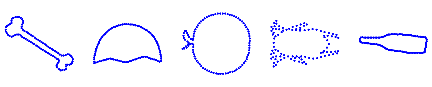
We consider three methodologies for classifying the shapes. In each experiment the same 80% of the shapes were used as a training set. In a completely naive approach, a support vector machine was trained on the permuted distance matrices. With this method, the classification rate on the testing set was 19%. In the second approach, one of the permuted distance training matrices $X$ was fixed and all other training matrices were aligned to $X$. The matrices were then “centered” on $X$, which can be understood as pulling them back to tangent vectors in $T_{[X]}$ via the log map (or, rather, the coupling-dependent log map $\log_{[X]}^{\mu}([Y])$ here). An SVM was then trained on these tangent vectors. Classification was tested by aligning and centering the test matrices with $X$, yielding a classification rate of 84%. In the final method, the Fréchet mean $\overline{X}$ of all samples in the training set was computed. Then all training matrices were aligned to $\overline{X}$ and pulled back to tangent vectors, where an SVM was trained. Classification was once again performed by aligning and centering test matrices with $\overline{X}$, where the classification rate was improved to 94%. This approach illustrates a template for vectorization of network data.

The Riemannian framework allows us to do other machine learning computations by pulling networks back to a tangent space; for example, we now present results of a tangent PCA experiment. Figure 6 illustrates the apple dataset that we used. Each shape is represented as a measure network as in the previous subsection. To perform tangent PCA, we first computed a Fréchet mean for these 20 shapes. Next we used log maps based at the chosen Fréchet mean to pull back the 20 shapes to vectors in the tangent space. Here we performed PCA as usual.

The first three principal directions explained 85% of the variance in the data, and they are visualized in Figure 7 via MDS embeddings. The first direction captures variance in the size of the apple; the second captures surface irregularities and the size and shape of the leaves, and the third captures the presence of a “bite” on the apple.

To illustrate our constructions on asymmetric networks, we generated a $100\times 100$ asymmetric stochastic block model (SBM) network $Y$ following the model provided in gwnets. Here $Y$ consisted of five blocks $B_{1},\ldots,B_{5}$ of 20 nodes each. For $y\in B_{i}$ and $y^{\prime}\in B_{j}$, we sampled $\omega_{Y}(y,y^{\prime})\sim N(\mu_{ij},5)$, where $\mu_{ij}\in\{0,25,50,75,100\}$. Negative values were allowed. See Figure 8 for an illustration of $Y$. Note that $Y$ is intuitively represented by a $5\times 5$ “ground-truth” matrix.

We averaged $Y$ with a $5\times 5$ all-zeros matrix $X$ using the network compression approach given in the supplementary materials to see if our method would recover the ground truth matrix. The output of our method is shown in the middle panel of Figure 8—up to a permutation (shown in the right panel), this accurately recovered the matrix of $\mu_{ij}$ values.

References

- (1) David Alvarez-Melis and Tommi Jaakkola. Gromov-Wasserstein alignment of word embedding spaces. In Proceedings of the 2018 Conference on Empirical Methods in Natural Language Processing, pages 1881–1890, 2018.
- (2) Luigi Ambrosio, Nicola Gigli, and Giuseppe Savaré. Gradient flows: in metric spaces and in the space of probability measures. Springer Science & Business Media, 2008.
- (3) David Bao, S-S Chern, and Zhongmin Shen. An introduction to Riemann-Finsler geometry, volume 200. Springer Science & Business Media, 2012.
- (4) Charlotte Bunne, David Alvarez-Melis, Andreas Krause, and Stefanie Jegelka. Learning generative models across incomparable spaces. In International Conference on Machine Learning, pages 851–861, 2019.
- (5) Dmitri Burago, Yuri Burago, and Sergei Ivanov. A course in metric geometry, volume 33. American Mathematical Soc., 2001.
- (6) Xin Chen and Jiming Peng. New analysis on sparse solutions to random standard quadratic optimization problems and extensions. Mathematics of Operations Research, 40(3):725–738, 2015.
- (7) Xin Chen, Jiming Peng, and Shuzhong Zhang. Sparse solutions to random standard quadratic optimization problems. Mathematical Programming, 141(1-2):273–293, 2013.
- (8) Samir Chowdhury and Facundo Mémoli. The gromov–wasserstein distance between networks and stable network invariants. Information and Inference: A Journal of the IMA, 8(4):757–787, 2019.
- (9) Samir Chowdhury and Tom Needham. Gromov-Wasserstein statistics Github repository. https://github.com/trneedham/gromov-wasserstein-statistics.
- (10) Marco Cuturi. Sinkhorn distances: Lightspeed computation of optimal transport. In Advances in Neural Information Processing Systems, pages 2292–2300, 2013.
- (11) Danielle Ezuz, Justin Solomon, Vladimir G Kim, and Mirela Ben-Chen. GWCNN: A metric alignment layer for deep shape analysis. In Computer Graphics Forum, volume 36, pages 49–57. Wiley Online Library, 2017.
- (12) Rémi Flamary and Nicolas Courty. POT: Python Optimal Transport library, 2017.
- (13) Xiaoyang Guo, Anuj Srivastava, and Sudeep Sarkar. A quotient space formulation for statistical analysis of graphical data. arXiv preprint arXiv:1909.12907, 2019.
- (14) Reigo Hendrikson. Using Gromov-Wasserstein distance to explore sets of networks. University of Tartu, Master Thesis, 2016.
- (15) Brijnesh J Jain and Klaus Obermayer. Structure spaces. Journal of Machine Learning Research, 10(Nov):2667–2714, 2009.
- (16) Brijnesh J Jain and Klaus Obermayer. Learning in Riemannian orbifolds. arXiv preprint arXiv:1204.4294, 2012.
- (17) Facundo Memoli. On the use of Gromov-Hausdorff Distances for Shape Comparison. In M. Botsch, R. Pajarola, B. Chen, and M. Zwicker, editors, Eurographics Symposium on Point-Based Graphics. The Eurographics Association, 2007.
- (18) Facundo Mémoli. Gromov-Wasserstein distances and the metric approach to object matching. Foundations of Computational Mathematics, pages 1–71, 2011. 10.1007/s10208-011-9093-5.
- (19) Facundo Mémoli and Tom Needham. Gromov-Monge quasi-metrics and distance distributions. arXiv preprint arXiv:1810.09646, 2018.
- (20) Mark Newman. Networks: an introduction. Oxford university press, 2010.
- (21) Jorge Nocedal and Stephen Wright. Numerical optimization. Springer Science & Business Media, 2006.
- (22) Xavier Pennec. Intrinsic statistics on riemannian manifolds: Basic tools for geometric measurements. Journal of Mathematical Imaging and Vision, 25(1):127, 2006.
- (23) Gabriel Peyré, Marco Cuturi, and Justin Solomon. Gromov-Wasserstein averaging of kernel and distance matrices. In International Conference on Machine Learning, pages 2664–2672, 2016.
- (24) Kaspar Riesen and Horst Bunke. IAM graph database repository for graph based pattern recognition and machine learning. In Joint IAPR International Workshops on Statistical Techniques in Pattern Recognition (SPR) and Structural and Syntactic Pattern Recognition (SSPR), pages 287–297. Springer, 2008.
- (25) Justin Solomon, Gabriel Peyré, Vladimir G Kim, and Suvrit Sra. Entropic metric alignment for correspondence problems. ACM Transactions on Graphics (TOG), 35(4):72, 2016.
- (26) Karl-Theodor Sturm. The space of spaces: curvature bounds and gradient flows on the space of metric measure spaces. arXiv preprint arXiv:1208.0434, 2012.
- (27) Vayer Titouan, Nicolas Courty, Romain Tavenard, and Rémi Flamary. Optimal transport for structured data with application on graphs. In International Conference on Machine Learning, pages 6275–6284, 2019.
- (28) Vayer Titouan, Rémi Flamary, Nicolas Courty, Romain Tavenard, and Laetitia Chapel. Sliced Gromov-Wasserstein. In Advances in Neural Information Processing Systems, pages 14726–14736, 2019.
- (29) Hongteng Xu, Dixin Luo, and Lawrence Carin. Scalable Gromov-Wasserstein learning for graph partitioning and matching. In Advances in Neural Information Processing Systems, pages 3046–3056, 2019.
- (30) Hongteng Xu, Dixin Luo, Hongyuan Zha, and Lawrence Carin. Gromov-Wasserstein learning for graph matching and node embedding. In International Conference on Machine Learning, pages 6932–6941, 2019.
Appendix A Derivation of Equation 1
To avoid overloading notation, write . In matrix form, we have:
Expanding the term inside the square root yields three terms. The first is the following:
Here the first equality followed by marginalization. Another term is as follows:
The final term is the only one that depends on :
The final equality holds by the definition of the Frobenius product, and this concludes the derivation of Equation 1.
We further note that in the special case where are symmetric positive definite, we can take a Cholesky decomposition to write:
Then we have:
where denotes the Frobenius norm. The function is now seen to be convex.
Appendix B Proofs
Proof of Proposition 3.
Let . Writing for the symmetrization of , we observe that
The computation then agrees with the computation in the symmetric setting of pcs16 after replacing with its symmetrization. ∎
Lemma 10.
Let be a finite measure network. Let . For , define as
Also let denote the diagonal coupling between and itself, i.e. the pushforward of under the diagonal map . Then we have:
Proof.
Consider the projection map defined by . It suffices to show that and . For the first assertion, let . Then we have:
For the second assertion, let . Suppose also . Then we have:
The conclusion follows because assigns zero measure to all pairs where . ∎
Proof of Proposition 5.
Let be a finite measure network and let for some . We wish to derive a condition which guarantees that
is a geodesic defined on . For any , lies in the same weak isomorphism class as
where denotes the diagonal coupling of with itself, as in Lemma 10. This is the general form of a geodesic given above (3). Moreover, , by the definition of . It therefore suffices to find a condition on which guarantees that is an optimal coupling between and the measure network