Robust Convergence Analysis of
Three-Operator Splitting

Three-operator splitting methods are aimed to solve optimization problems of the form

where $f,g$ and $h$ are proper, closed and convex and $h$ is Lipschitz differentiable. Problems of the form (1) encompass a variety of problems in signal processing, control, and machine learning, such as group LASSO [1], support vector machines [2], matrix completion [3] and optimal control [4].

To solve (1), [5] proposed the three-operator splitting (TOS) method outlined below.

Related Work. To solve problems of the form (1) with two or more nonsmooth terms, several splitting methods have been proposed. For example, [6, 7] propose a generalized forward-backward splitting algorithm which weakly converges to the minimizer of (1). A primal-dual method based on reformulating (1) as a saddle point problem has been proposed by [8, 9, 10, 11, 12]. [12, 13] and [5] prove the $O(1/k)$ ergodic convergence rate on the saddle point suboptimality and function value suboptimality, respectively. When both $f(x)$ and $h(x)$ are Lipschitz differentiable, [5, 12] give an $O(1/k)$ convergence proof in terms of the objective function value suboptimality. Furthermore, they derive linear convergence under stronger assumptions.

Recently, there has been a surge of interest in analysis and design of optimization algorithms using robust control and semidefinite programming [14, 15, 16, 17, 18, 19, 20, 21]. The main idea is to view the worst-case convergence analysis of optimization algorithms as robust stability analysis of a linear dynamical system in feedback connection with an uncertain component [14]. This perspective is useful in that it allows us to provide either new bounds or design new optimization algorithms in a systematic manner.

Our Contribution. The TOS Algorithm can be viewed as a linear dynamical system driven by the nonlinear operators $\mathrm{prox}_{\alpha f},\mathrm{prox}_{\alpha g}$ and $\nabla h$. For analyzing the convergence of the algorithm to its fixed point(s), we use the framework of quadratic constraints to abstract these nonlinearities using the assumptions made about the oracle models of $f,g$ and $h$. We then define a Lyapunov function for the algorithm whose decrease along the trajectories directly certifies convergence to an optimal solution at a specific rate. We then find sufficient conditions, in terms of matrix inequalities, to guarantee this decrease condition. Depending on the regularity assumptions, we provide this convergence rate in terms of either the distance to the optimal solution, the norm of the optimality residual, or the objective value. These matrix inequalities can be used to select the parameters for optimal worst-case performance.

The rest of the paper is organized as follows. In Section II, we provide preliminaries and background. Then we analyze the sublinear and linear convergence of the algorithm under different sets of assumptions in Section III and Section IV, respectively. In Section V, we solve an optimal control problem to illustrate our analysis of convergence and parameter selection. Section VI concludes the paper.

We denote by $I_{d}$ the $d$-dimensional identity matrix. For a function $f:\mathbb{R}^{d}\rightarrow\mathbb{R}$, the domain of $f$ is $\text{dom}\ f=\{x\in\mathbb{R}^{d}\mid f(x)<\infty\}$. The subdifferential of a convex function $f$ at point $x$ is the set $\partial f(x)=\{g\in\mathbb{R}^{d}\mid f(y)-f(x)\geq g^{T}(y-x),\forall y\in\text{dom}\ f\}$. With abuse of notation, we will denote $\partial f(x)$ as the subgradient of $f$ which is an element of the subdifferential of $f$ at $x$ as well. In this paper, unless explicitly specified otherwise, the norm $||x||$ of a vector $x$ denotes the $2$-norm of $x$. We denote the Kronecker product by $\otimes$ and the set of $d\times d$ symmetric matrices by $\mathbb{S}^{d}$. The spectral norm (maximum singular value) of a matrix $X$ is denoted by $\lVert X\rVert_{2}$.

We denote the function class satisfying (3) and (4) by $\mathcal{F}(m_{f},L_{f})$. When $f$ is not differentiable, we have $L_{f}=\infty$ and we adopt the convention $1/L_{f}=0$.

A differentiable function $f$ belongs to the class $\mathcal{F}(m,L)$ on $\mathcal{S}$ if and only if the gradient function $\nabla f$ satisfies the incremental quadratic constraint in (5) where $Q=Q(m,L)$ is given by [23, 14]

The TOS algorithm achieves linear convergence rate if there exists a $\rho\in(0,1)$ such that $\lVert z^{k}-z^{\star}\rVert\leq\mathcal{O}(\rho^{k})$ for all $k$. In [5], it has been proved that the TOS algorithm achieves linear convergence rate under the following assumption.

A closed-form representation of an upper bound on the convergence rate is given in [5]. However, the form of this bound is complicated and not tight. In [25] the authors improved the upper bound on $\rho$ by formulating an SDP. In contrast, we use Lyapunov functions and incremental quadratic constraints to formulate an SDP that bounds $\rho$ and compare the results with those of [25]

To begin, we use the following quadratic Lyapunov function:

If there exists a $\rho\in(0,1)$ such that $V_{k+1}\leq\rho^{2}V_{k}$ holds for all $k>0$, then the algorithm is exponentially convergent.

The following theorem provides a sufficient condition in terms of a matrix inequality to achieve linear convergence of the TOS algorithm.

Note that the matrix inequality in (15) is linear in all the parameters except for $\alpha$ and $\lambda$. We can use the same technique as shown in Section III-B to transform (15) into an LMI when the stepsize $\alpha$ is fixed. Let

and

Then by Schur complement, (15) is satisfied if and only if

Therefore, for a given stepsize $\alpha$, the best convergence rate can be found by solving the following SDP:

Denote the optimal solution to (17) by $\rho^{\star}(\alpha)$. Then by a grid search of $\alpha>0$, we can find the optimal bound $\rho^{\star}$ and the optimal stepsize $\alpha^{\star}$ through

In Fig. 2, we plot $\alpha\mapsto\rho^{\star}(\alpha)^{2}$ and contrast it with the bounds of [25] for various regularity assumptions on $F$. We see from this figure that numerically we achieve the same bounds as in [25]. In fact, as shown in Appendix A-D, the formulation in (17) is the dual of the SDP developed in [25].

In this section, we validate the parameter selection procedure in Section III-A with a box constrained quadratic optimal control problem from [2, Sec. IV. A]:

where $Q_{t}\succeq 0$ and $R_{t}\succ 0$. We use $x=[x_{0}^{T}\ \cdots\ x_{N}^{T}]^{T}\in\mathbb{R}^{(N+1)n}$ and $u=[u_{0}^{T}\ \cdots\ u_{N-1}^{T}]^{T}\in\mathbb{R}^{Nm}$ to denote the concatenated states and control inputs, and $w=[x^{T}\ u^{T}]^{T}\in\mathbb{R}^{(N+1)n+Nm}$ to denote the state-control trajectory.

Define the set of state-control pairs that satisfy the dynamics of (18) as

and the set of state-control constraints as

The indicator function $I_{\mathcal{D}}$ is defined by

and $I_{\mathcal{C}}$ is defined similarly. Then the box constrained optimal control problem (18) can be expressed as

where

Let $f(w)=I_{\mathcal{C}}(w),g(w)=I_{\mathcal{D}}(w)$ and $h(w)=\frac{1}{2}w^{T}Ew$. It can be easily checked that $f,g$ and $h$ are proper, closed and convex and $h$ is Lipschitz differentiable. Then (19) can be viewed as a three-operator splitting problem and falls into the one Lipschitz operator category in Section III-A.

We consider a medium-size optimal control problem for illustration. For simplicity, we apply a linear time-invariant system with $x_{t}\in\mathbb{R}^{20},u\in\mathbb{R}^{5},A_{t}=A,B_{t}=B$ and constant $Q_{t}=Q,R_{t}=R$. The horizon length is $N=20$. The data are all generated randomly and the matrix $A$ is scaled to be marginally stable, i.e., the largest magnitude of the eigenvalue of $A$ is one.

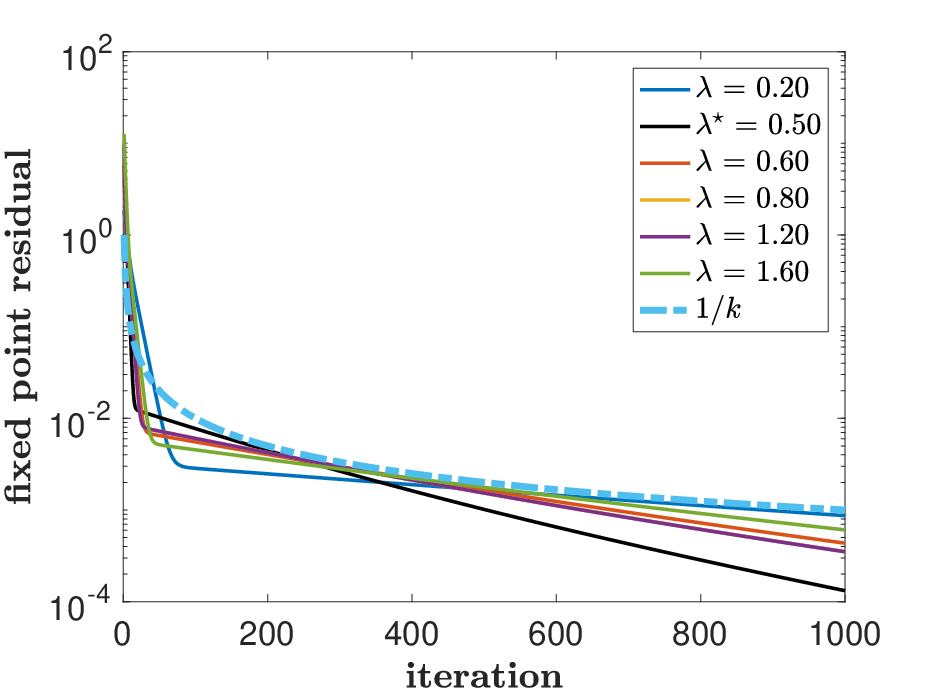
According to Remark 1, $\lambda=\frac{1}{2}$ gives the fastest worst-case convergence. We solve the problem (19) using the TOS algorithm with different values of $\lambda$ and stepsizes $\alpha=(2-\lambda)/L_{h}$, where $L_{h}$ equals to the spectral norm of matrix $E$ in this example. Fig. 3 shows that all convergence rates are dominated by $1/k$ and $\lambda=\frac{1}{2}$ yields the fastest convergence as expected.

In this paper, we proposed a unified framework, based on Lyapunov functions and quadratic constraints, for convergence rate analysis and parameter selection of the three-operator splitting algorithm [5]. Under different regularity assumptions of the objective function, this approach can certify sublinear/linear convergence of the algorithm. In particular, we showed that our bounds are tight for the case of linear convergence.

References

• [1] L. Jacob, G. Obozinski, and J.-P. Vert, “Group lasso with overlap and graph lasso,” in Proceedings of the 26th annual international conference on machine learning, pp. 433–440, ACM, 2009.
• [2] B. O’Donoghue, G. Stathopoulos, and S. Boyd, “A splitting method for optimal control,” IEEE Transactions on Control Systems Technology, vol. 21, no. 6, pp. 2432–2442, 2013.
• [3] E. J. Candes and Y. Plan, “Matrix completion with noise,” Proceedings of the IEEE, vol. 98, no. 6, pp. 925–936, 2010.
• [4] G. Stathopoulos, H. Shukla, A. Szucs, Y. Pu, C. N. Jones, et al., “Operator splitting methods in control,” Foundations and Trends in Systems and Control, vol. 3, no. 3, pp. 249–362, 2016.
• [5] D. Davis and W. Yin, “A three-operator splitting scheme and its optimization applications,” Set-valued and variational analysis, vol. 25, no. 4, pp. 829–858, 2017.
• [6] H. Raguet, J. Fadili, and G. Peyré, “A generalized forward-backward splitting,” SIAM Journal on Imaging Sciences, vol. 6, no. 3, pp. 1199–1226, 2013.
• [7] H. Raguet and L. Landrieu, “Preconditioning of a generalized forward-backward splitting and application to optimization on graphs,” SIAM Journal on Imaging Sciences, vol. 8, no. 4, pp. 2706–2739, 2015.
• [8] L. Condat, “A primal–dual splitting method for convex optimization involving lipschitzian, proximable and linear composite terms,” Journal of Optimization Theory and Applications, vol. 158, no. 2, pp. 460–479, 2013.
• [9] B. C. Vũ, “A splitting algorithm for dual monotone inclusions involving cocoercive operators,” Advances in Computational Mathematics, vol. 38, no. 3, pp. 667–681, 2013.
• [10] Q. Li and N. Zhang, “Fast proximity-gradient algorithms for structured convex optimization problems,” Applied and Computational Harmonic Analysis, vol. 41, no. 2, pp. 491–517, 2016.
• [11] M. Yan, “A new primal–dual algorithm for minimizing the sum of three functions with a linear operator,” Journal of Scientific Computing, vol. 76, no. 3, pp. 1698–1717, 2018.
• [12] F. Pedregosa and G. Gidel, “Adaptive three operator splitting,” arXiv preprint arXiv:1804.02339, 2018.
• [13] A. Chambolle and T. Pock, “On the ergodic convergence rates of a first-order primal–dual algorithm,” Mathematical Programming, vol. 159, no. 1-2, pp. 253–287, 2016.
• [14] L. Lessard, B. Recht, and A. Packard, “Analysis and design of optimization algorithms via integral quadratic constraints,” SIAM Journal on Optimization, vol. 26, no. 1, pp. 57–95, 2016.
• [15] M. Fazlyab, A. Ribeiro, M. Morari, and V. M. Preciado, “Analysis of optimization algorithms via integral quadratic constraints: Nonstrongly convex problems,” SIAM Journal on Optimization, vol. 28, no. 3, pp. 2654–2689, 2018.
• [16] B. Hu and L. Lessard, “Dissipativity theory for nesterov’s accelerated method,” in Proceedings of the 34th International Conference on Machine Learning-Volume 70, pp. 1549–1557, JMLR. org, 2017.
• [17] B. Van Scoy, R. A. Freeman, and K. M. Lynch, “The fastest known globally convergent first-order method for minimizing strongly convex functions,” IEEE Control Systems Letters, vol. 2, no. 1, pp. 49–54, 2017.
• [18] M. Fazlyab, M. Morari, and V. M. Preciado, “Design of first-order optimization algorithms via sum-of-squares programming,” in 2018 IEEE Conference on Decision and Control (CDC), pp. 4445–4452, IEEE, 2018.
• [19] J. H. Seidman, M. Fazlyab, V. M. Preciado, and G. J. Pappas, “A control-theoretic approach to analysis and parameter selection of douglas–rachford splitting,” IEEE Control Systems Letters, vol. 4, no. 1, pp. 199–204, 2019.
• [20] H. Mohammadi, M. Razaviyayn, and M. R. Jovanović, “Performance of noisy nesterov’s accelerated method for strongly convex optimization problems,” in 2019 American Control Conference (ACC), pp. 3426–3431, IEEE, 2019.
• [21] S. Hassan-Moghaddam and M. R. Jovanović, “Proximal gradient flow and douglas-rachford splitting dynamics: global exponential stability via integral quadratic constraints,” arXiv preprint arXiv:1908.09043, 2019.
• [22] B. Açıkmeşe and M. Corless, “Observers for systems with nonlinearities satisfying incremental quadratic constraints,” Automatica, vol. 47, no. 7, pp. 1339–1348, 2011.
• [23] Y. Nesterov, “Introductory lectures on convex programming,” 1998.
• [24] R. A. Horn and C. R. Johnson, Matrix analysis. Cambridge university press, 2012.
• [25] E. K. Ryu, A. B. Taylor, C. Bergeling, and P. Giselsson, “Operator splitting performance estimation: Tight contraction factors and optimal parameter selection,” arXiv preprint arXiv:1812.00146, 2018.