Staccato radiation from the decay of large amplitude oscillons
Abstract
We study the decay of large amplitude, almost periodic breather-like states in a deformed sine-Gordon model in one spatial dimension. We discover that these objects decay in a staggered fashion via a series of transitions, during which higher harmonics are released as short, staccato bursts of radiation. Further, we argue that this phenomenon is not restricted to one particular model, and that similar mechanisms of radiative decay of long-lived oscillating states can be observed for a wide class of physical systems, including the model.
Keywords:
oscillons, relaxation, nearly-integrabilityMany non-linear physical systems support oscillons, spatially localized almost time-periodic field configurations which can live for exceptionally long times [1, 2, 3]. Unlike the breathers of the sine-Gordon (sG) model, oscillons (sometimes also referred to as quasi-breathers) continuously emit scalar radiation via the excitation of scattering modes of the continuous spectrum. Oscillons and their close relatives, gravitationally bound oscillatons, appear in a broad class of classical field theories in various dimensions, and in recent years they have attracted much attention [4, 5, 6, 7, 8, 9, 10].
In 1+1 dimensional scalar field theories, the slow decrease of the amplitude of small oscillons continues smoothly up to the limit of very small size. However, and despite the fact that its amplitude becomes arbitrarily small, the oscillon can never be described as a solution of a linearized equation in the vacuum sector, since its existence depends on the nonlinearity of the system. Sine-Gordon breathers possess exactly the same feature, and the similarity between the perfectly periodic, non-radiating sG breathers and oscillon solutions of the theory leads to interesting relationships between the two, something that we will exploit in this paper. It is worth mentioning that modified sG models, and variants including the and theories, have many physical applications and have been studied for many decades [11, 12, 13, 14, 15, 16, 17, 18]. Nevertheless, we were able to find the novel phenomenon of stacatto decay, as described in this paper.
The decay rate of small-amplitude oscillons in nonintegrable models such as the model has been explored in a number of works, including [19, 20, 21, 22]. It was found to be beyond all orders in perturbation theory, given by , where is the energy of the oscillon and is a constant. The long time evolution of the small-amplitude oscillon thus involves the slow decrease of its amplitude, which turns out to be accompanied by a gradual increase in its frequency. Nevertheless, the frequency remains below the mass threshold, meaning that the modes of the continuum can only be excited through the second (and higher) harmonics [21, 23, 24]. In higher spatial dimensions, the configuration may rapidly collapse into radiation as the fundamental frequency approaches some critical value, which is still below the mass threshold [21, 23, 24, 25, 26, 27]. However, and despite many extensive numerical studies, there is still very little known about the true nature of this decay process.
In contrast to previous studies, our focus here is not on small amplitude oscillons, but rather on large oscillons, taking a mildly deformed 1+1 dimensional sG model with weak integrability breaking as our main example. This deformation lifts the infinite degeneracy of the vacuum while leaving a symmetry unbroken. We have found that the long time evolution of the corresponding oscillon configuration is not smooth, but is realised through a series of transitions caused by the release of higher propagating harmonics. In previous work [28, 29] we found that deep, oscillating bound modes, when excited to the nonlinear regime, can, in certain circumstances, block one or more harmonics as possible decay channels. This phenomenon depends on the nonlinear dependence between frequency and amplitude, which in the previously studied models could be found only numerically, or within perturbation theory. Breathers, on the other hand, are perfect examples of such nonlinear excitations, and for suitably small deviations from integrability they well approximate the decaying oscillon. Their frequency-amplitude relation is well known analytically. Moreover, the frequency can be changed, due to the nonlinearities, within the entire mass gap. By breaking the integrability we allow the oscillons to radiate and evolve through a wide range of frequencies.
A deformed sine-Gordon model. Consider a scalar field theory in 1+1 dimensions defined by the Lagrangian
| (1) |
where is a simple -breaking modification of the sG potential depending on a parameter :
| (2) |
The standard sG potential is recovered in the limit , while setting yields a potential with just two vacua, and , a shift and rescaling of the -symmetric potential of the model. Thus, the model with the potential (2) interpolates between the integrable sG model and the model, with integrability being broken for all non-zero values of . Note that the parameters in (2) are fixed in such a way that the mass of small perturbations around the vacuum remains the same as in the original sG model, since for all values of .
The sG model supports a spatially localized solution, exactly periodic in time, the breather:
| (3) |
where . The topological charge of this configuration is zero, and it can be viewed as a bound state of a kink and anti-kink, oscillating with a constant frequency , which is a parameter of the solution. Although is a function of the frequency , we leave the dependence on explicit to distinguish which part of the solution is associated with the profile and which with the time evolution.
Our goal is to study the time evolution of the breather configuration (3) in the deformed model (2).
Note that in the pure sG model, the breather solution can be decomposed into a Fourier series in time with only odd multiplicities of the frequency . Since the deformed potential (2) is no longer invariant with respect to parity reflections about either vacuum, the corresponding expansion for should also include even harmonics.
The oscillon solutions of the theory have been studied in many papers, including [19, 20, 21, 23, 24]. When the amplitude of the oscillations is small, a oscillon can be treated as a small sG breather perturbed by higher order polynomial terms in the potential. Evidently, this deformation breaks the integrability of the sG system and causes the radiative decay of the oscillon.
In this paper we consider a different limit. We assume that the amplitude is large, but the modification of the sG potential is small, . We conjecture that in such a case the profile of the oscillon can be well approximated by the sG breather, thus the initial data in our numerical simulation corresponds to the configuration (3)
| (4) |
for some initial frequency , with .
Numerical simulations. We have solved the full nonlinear evolution partial differential equation numerically, taking the breather profile (3) as the initial condition at . Large amplitude oscillons with radiated visibly even for relatively small values of the integrability breaking parameter, . We measured the field values at the centre , and far away from the oscillon, . An example evolution for and is shown in the Figure 1 (see – and hear – also the Supplementary Material [A] and [B]). Subplot (a) shows the field at the centre, (b) the field at a distance from the centre and (c) the spectrogram of the field measured at the centre.
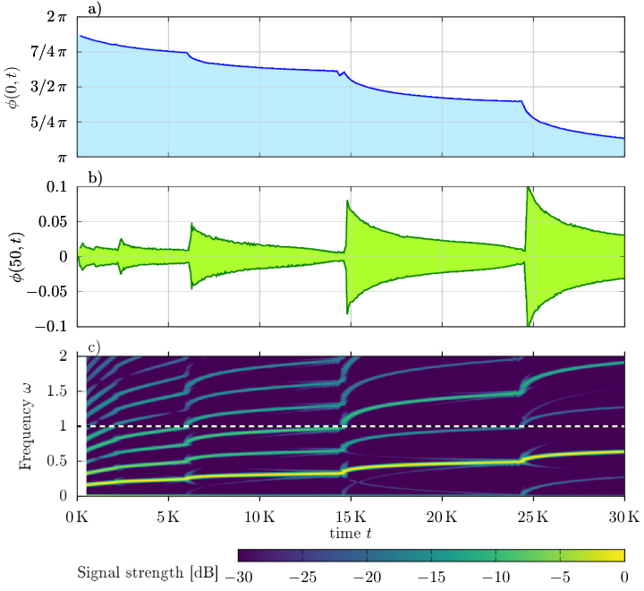
The most striking feature of the evolution is that the oscillon does not relax uniformly (Figure 1(a)). Relatively long times of what looks like the standard relaxation processes are separated by sudden sharp jumps, during which the rate of the decay increases significantly. These jumps are reflected in far-field measurements (Figure 1(b)) as larger bursts of radiation, by at least one order of magnitude. The spectrogram (c) gives more insight into the nature of these jumps. Bright lines correspond to dominant frequencies in the spectrum. Notably, the lowest, basic, frequency is accompanied by all of its multiples. After a short transient time of some adjustment, at least six harmonics are visible below the mass threshold. For most of the time the basic frequency and the higher harmonics change adiabatically slowly. A jump occurs whenever one of the harmonics crosses the value , which is the mass threshold. The frequency of the oscillon quickly changes and then slows down until the next event. During these short transitions the harmonic entering the scattering spectrum changes its nature from localized to wave-like. This explains the burst of radiation observed in the far field.
Stationary approach. Numerical simulations suggest that the oscillon for most of the time evolves adiabatically, slowly changing its basic frequency and amplitude. It is therefore justified to assume that, in between the jumps, the momentary state of an oscillon can be well approximated by a stationary solution, which is just small perturbation of a breather. Let us consider a perturbative expansion of the field equation
| (5) |
around the breather solution (3), . The deformation of the usual sG potential defined by (2) is of the first order in ,
| (6) |
In the first order in the corresponding equation of motion is
| (7) |
Here
| (8) |
Note that the partial differential equation (7) resembles the well known Mathieu or Hill equation with additional driving force .
The breather solution is periodic in time, and the spectrogram of the oscillon field at its centre shows that it is almost periodic, with a well defined basic frequency and its multiples. Therefore we can make use of the Fourier decomposition
| (9) |
where , and
| (10) |
Substituting these expansions into the first order equation (7), we obtain
| (11) |
This is a system of linear, coupled ODEs, which describes the evolution of the modes , coupled via the convolution of infinite vectors and . The solutions to equation (11) for different harmonics can be categorised as either normalizable modes with , which are localized by the potential , or radiative modes above the mass threshold, . The latter modes represent outgoing waves, and satisfy the following boundary condition for
| (12) |
which ensures the absence of the incoming waves.
The normalizable Fourier modes () must vanish exponentially at spatial infinity as . The asymptotic boundary condition for these modes is
| (13) |
We solved the above problem by discretising the system (11) and making use of the fourth order finite difference scheme with even boundary conditions imposed at . Example solution is plotted in Firgure 2.
From these solutions we can extract the amplitudes of the corresponding modes , defined as
| (14) |
The amplitudes for the first few harmonics are shown in Figure 3, where the Fourier series were truncated to include forty modes.
Note that one can clearly see the large amplitude peaks of the localized modes at the resonance frequencies , . These peaks correspond to the situation when one of the multiplicities of the basic frequency changes its nature from localized to propagating . Exactly at the wave number vanishes, . The stationary approach described by equation (11) is unable to describe this situation properly due to the resonance between one of the harmonics and the mass threshold. This singularity shows the limitations of the perturbative approach and indicates that for these special cases the evolution is highly non-perturbative. However, in between those resonant frequencies , the evolution should be properly described by the Fourier decomposition, at least in the adiabatic approximation assuming that the frequency changes very slowly with time, which is true for small values of . On the other hand, for all nonvanishing the oscillon should undergo a dramatic, non-perturbative change in its structure (one of the harmonics delocalizes) in a close vicinity of the resonant frequencies.
One of the interesting features of the radiation bursts is their characteristic structure, which allows the harmonic from which they came to be identified. For example if the ratio of the first two observed frequencies is (a perfect fifth in musical terminology), the second harmonic of the oscillon was released. If the ratio is (a perfect fourth), then the third harmonic was released and the second is still below the threshold (see and hear also the Supplementary Material [A] and [B]).
We have also investigated how the above patters change for different values of . In the Figure 4 we have plotted the number of the first propagating harmonics as a function of the perturbation parameter and evolution time, starting from the large amplitude sG breather configuration with frequency . Note that the frequency of the oscillations can be measured numerically only when the oscillating field possess an extremum at , which is generally not a case. We have interpolated the frequency for much denser time gird using cubic splines.
The perturbation destroys the integrability of the model, thus even for a very small values of the oscillon radiates the outgoing waves reducing its amplitude and, consequently, releasing lower harmonics. Even for relatively small value , after about units of time the oscillon relaxes radiation through the second harmonic, which becomes visible in the power spectrum. For smaller values of the time between the transitions increases significantly. Moreover a resonant structure is clearly visible, however the time evolution becomes much slower for some values of .
More generally, we observe that the pattern of time evolution of the radiating oscillon in the perturbed model (2) is very sensitive to the small variations of revealing some chaotic behaviour. Note that similar feature was observed by Gleiser for the 3+1 dimensional oscillons [3], it was pointed out that some initial data produced exceptionally long living oscillons while a tiny variation of the input profile lead to abrupt collapse of the configuration.

Generalisations. Further numerical simulations of our model show that for larger values of , closer to the limit, the increased coupling to radiation means that the oscillons reduce in amplitude more quickly, impeding the observation of transitions (even for , the amplitude reduces to the point where the frequency is above after just units of time). However, it is not hard to find other models where similar features are visible, including the much-discussed model [17, 18, 30]. In the triply-degenerate vacuum case that was the focus of [18, 30], after a low-velocity collision of a kink and an antikink, a bound state (often called a bion) is formed. This object radiates and loses energy, slowly decaying to vacuum as an oscillon. We have repeated the same analysis as above (Figure 5 and the Supplementary Material [C] and [D]) for this case, looking at the collision between a right-moving kink interpolating between the and vacua, and a left-moving antikink interpolating between the and vacua, and found that even here, relatively far from the sG model, the evolution is very similar (see figure 5 and the Supplementary Material [C] and [D]). The oscillon, although highly perturbed, decays through a series of jumps which can easily be matched with the successive releases of higher harmonics. In the spectrogram some more frequencies are also visible due to the initial perturbations, but the dominant features come from the effects described in this paper. Provided the lifting of the vacuum degeneracy is not too great, the same phenomena can be seen in the more-general models originally discussed in [17]. As a final example, we investigated the hyperbolic model recently introduced in [31], and found similar effects there too, as shown in the Figure 6.


Conclusions. In this paper we presented a novel approach to the analysis of oscillons in which we treated large oscillons as perturbed breathers in slightly deformed sG model. As our example we took a potential which interpolates between the infinitely-degenerate and -symmetric sG potential and the doubly-degenerate potential of a scaled model. An arbitrarily-small deformation of the sG system breaks both the integrability and the symmetry of the system, and transforms the exact time-periodic non-radiating breather into an oscillon. The cores of these oscillating lumps are very similar to the cores of sG breathers, but they possess a radiating tail. One of the surprising things we found is that a system which is so close to an integrable model can behave in such a complicated way (though see [32] for a further example of an apparently small breaking of integrability having a dramatic effect on a system’s behaviour). The evolution is also very different from the decay of the usual, small-amplitude oscillons, extensively studied in the literature in many models. Counterintuitively, the large-amplitude oscillons do not decay uniformly but rather through a series of radiative bursts of increasing amplitude. These bursts can be associated with the release of successive harmonics into the continuous spectrum. Only after the releasing the second lowest harmonic do the oscillons enter a regular decay phase.
We also discovered a similar type of staggered relaxation in the and hyperbolic models, in the decay of an oscillon created by the annihilation of a kink and an antikink. It is natural to predict that similar phenomena will be observed in many other models, including those in which the integrability of the sG model is broken by other field-theoretic potentials, external potentials (or impurities), or modified boundary conditions (including Neumann [28] and Robin [32]). We therefore expect that the effects described in this paper will arise in a wide class of field theories, once large-amplitude excitations are considered.
Finally, we mention that non-uniform oscillon decays have been observed in some earlier studies of oscillons in higher dimensions [24, 27]. However, these appear to be very different from the decays we have discussed in this paper. For example, the three-dimensional oscillon decay shown in figure 6 of [24] is not fully uniform, pulses of radiation initially being released in sync with a large period modulation of the amplitude of the field at the origin. However this modulation is not itself associated with the successive crossing of thresholds, as was the case for our models. This form of decay continues until a certain critical frequency is reached, at which point the oscillon of [24] becomes unstable and decays more quickly, releasing a large amount of radiation. The lifetime of this oscillon depends on the initial conditions, revealing an intriguing resonant structure. However, in these earlier studies, only oscillons with high frequency, just below the mass threshold, were considered. All harmonics except the zeroth-frequency and the basic one were already above the mass threshold. The observed final jump of the decay rate was due to the oscillon entering an unstable phase, when its size was not sufficient for nonlinearities to bind the field into a single localized object. We, on the other hand, studied low frequency oscillons when the jumps in the decay rate corresponded to the sequential releasing of higher harmonics as the frequency gradually increased. Moreover, in one spatial dimension we would not expect an oscillon to end its evolution with a collapse after reaching some critical frequency, but rather to decay slowly into the vaccum. This is indeed what we observed in our models after the final stacatto burst of radiation was released.
Acknowledgements. TR wishes to thank Piotr Bizoń for many inspiring discussions. Ya.S. gratefully acknowledges partial support of the Ministry of Science and Higher Education of Russian Federation, project No 3.1386.2017. This project has also received funding from the European Union’s Horizon 2020 research and innovation programme under the Marie Skodowska-Curie grant agreement No. 764850, “SAGEX”, and from the STFC under consolidated grant ST/P000371/1.
Supplementary material. The files accompanying this paper illustrate a few aspects of large oscillon decay. In each of the audio-visual files [A] – [D], there are four plots: a spectrogram (upper-left), the field either at the centre or at (bottom-left), a current FFT of a short window (upper-right) and a current view of the time dependence of the field (bottom-right). We have added soundtracks to these plots, inspired in part by the LIGO audio files [33]. These soundtracks “audibilize" the oscillations of the field, with the frequency adjusted for the human ear. In the far-field soundtracks the characteristic bell-like sounds signal the passages of the staccato bursts of radiation past the measuring point.
- [A]
OscillonCentre.mov : Evolution of the field at the centre for , .
- [B]
OscillonFar.mov : Evolution of the field at for , .
- [C]
Phi6Centre.mov : Evolution of the field at the centre after a kink-antikink collision in the model.
- [D]
Phi6Far.mov : Evolution of the field at after a kink-antikink collision in the model.
References
- Bogolyubsky and Makhankov [1976] I. Bogolyubsky, V. Makhankov, On the pulsed soliton lifetime in two classical relativistic theory models, JETP Lett. 24 (1976) 12.
- Copeland et al. [1995] E. J. Copeland, M. Gleiser, H.-R. Müller, Oscillons: Resonant configurations during bubble collapse, Phys. Rev. D 52 (1995) 1920. URL: https://doi.org/10.1103/PhysRevD.52.1920.
- Gleiser [1994] M. Gleiser, Pseudostable bubbles, Phys. Rev. D 49 (1994) 2978. URL: https://doi.org/10.1103/PhysRevD.49.2978.
- Riotto [1996] A. Riotto, Are oscillons present during a first order electroweak phase transition?, Phys. Lett. B365 (1996) 64–71. doi:10.1016/0370-2693(95)01239-7. arXiv:hep-ph/9507201.
- Umurhan et al. [1998] O. M. Umurhan, L. Tao, E. A. Spiegel, Stellar oscillons, Annals N. Y. Acad. Sci. 867 (1998) 298. doi:10.1111/j.1749-6632.1998.tb11265.x. arXiv:astro-ph/9806209.
- Farhi et al. [2005] E. Farhi, N. Graham, V. Khemani, R. Markov, R. Rosales, An Oscillon in the SU(2) gauged Higgs model, Phys. Rev. D72 (2005) 101701. doi:10.1103/PhysRevD.72.101701. arXiv:hep-th/0505273.
- Gleiser [2007] M. Gleiser, Oscillons in scalar field theories: Applications in higher dimensions and inflation, Int. J. Mod. Phys. D16 (2007) 219–229. doi:10.1142/S0218271807009954. arXiv:hep-th/0602187.
- Alcubierre et al. [2003] M. Alcubierre, R. Becerril, S. F. Guzman, T. Matos, D. Nunez, L. A. Urena-Lopez, Numerical studies of -oscillatons, Class. Quant. Grav. 20 (2003) 2883–2904. doi:10.1088/0264-9381/20/13/332. arXiv:gr-qc/0301105.
- Graham [2007] N. Graham, An Electroweak oscillon, Phys. Rev. Lett. 98 (2007) 101801. doi:10.1103/PhysRevLett.98.101801,10.1103/PhysRevLett.98.189904. arXiv:hep-th/0610267, [Erratum: Phys. Rev. Lett. 98, 189904 (2007)].
- Fodor et al. [2010] G. Fodor, P. Forgacs, M. Mezei, Mass loss and longevity of gravitationally bound oscillating scalar lumps (oscillatons) in D-dimensions, Phys. Rev. D81 (2010) 064029. doi:10.1103/PhysRevD.81.064029. arXiv:0912.5351.
- Cuevas et al. [2009] J. Cuevas, L. Q. English, P. G. Kevrekidis, M. Anderson, Discrete breathers in a forced-damped array of coupled pendula: Modeling, computation, and experiment, Phys. Rev. Lett. 102 (2009) 224101. URL: https://link.aps.org/doi/10.1103/PhysRevLett.102.224101. doi:10.1103/PhysRevLett.102.224101.
- Kivshar and Malomed [1989] Y. S. Kivshar, B. A. Malomed, Dynamics of solitons in nearly integrable systems, Rev. Mod. Phys. 61 (1989) 763–915. URL: https://link.aps.org/doi/10.1103/RevModPhys.61.763. doi:10.1103/RevModPhys.61.763.
- Cuevas-Maraver and Kevrekidis [2019] J. Cuevas-Maraver, P. G. Kevrekidis, Discrete Breathers in and Related Models, Springer International Publishing, Cham, 2019, pp. 137–162. URL: https://doi.org/10.1007/978-3-030-11839-6_7. doi:10.1007/978-3-030-11839-6_7.
- Cuevas-Maraver et al. [2014] J. Cuevas-Maraver, P. G. Kevrekidis, F. Williams (Eds.), The sine-Gordon Model and its Applications: From Pendula and Josephson Junctions to Gravity and High-Energy Physics, Springer International Publishing, Cham, 2014, pp. 1–30.
- Gulevich et al. [2012] D. R. Gulevich, M. B. Gaifullin, F. V. Kusmartsev, Controlled dynamics of sine-gordon breather in long josephson junctions, The European Physical Journal B 85 (2012) 24. URL: https://doi.org/10.1140/epjb/e2011-20689-4. doi:10.1140/epjb/e2011-20689-4.
- Flach and Willis [1998] S. Flach, C. Willis, Discrete breathers, Physics Reports 295 (1998) 181 – 264. URL: http://www.sciencedirect.com/science/article/pii/S0370157397000689. doi:https://doi.org/10.1016/S0370-1573(97)00068-9.
- Christ and Lee [1975] N. H. Christ, T. D. Lee, Quantum expansion of soliton solutions, Phys. Rev. D 12 (1975) 1606–1627. URL: https://link.aps.org/doi/10.1103/PhysRevD.12.1606. doi:10.1103/PhysRevD.12.1606.
- Lohe [1979] M. A. Lohe, Soliton structures in , Phys. Rev. D 20 (1979) 3120–3130. URL: https://link.aps.org/doi/10.1103/PhysRevD.20.3120. doi:10.1103/PhysRevD.20.3120.
- Segur and Kruskal [1987] H. Segur, M. D. Kruskal, Nonexistence of small-amplitude breather solutions in theory, Phys. Rev. Lett. 58 (1987) 747. URL: https://doi.org/10.1103/PhysRevLett.58.747.
- Boyd [1995] J. P. Boyd, Weakly nonlocal envelope solitary waves: numerical calculations for the Klein-Gordon () equation, Wave Motion 21 (1995) 311 – 330. URL: http://www.sciencedirect.com/science/article/pii/0165212595000054. doi:https://doi.org/10.1016/0165-2125(95)00005-4.
- Fodor et al. [2009] G. Fodor, P. Forgacs, Z. Horváth, M. Mezei, Computation of the radiation amplitude of oscillons, Phys. Rev. D 79 (2009) 065002. URL: https://doi.org/10.1103/PhysRevD.79.065002.
- Fodor [2019] G. Fodor, A review on radiation of oscillons and oscillatons, Ph.D. thesis, Wigner RCP, Budapest, 2019. arXiv:1911.03340.
- Hindmarsh and Salmi [2008] M. Hindmarsh, P. Salmi, Oscillons and domain walls, Phys. Rev. D 77 (2008) 105025. URL: https://doi.org/10.1103/PhysRevD.77.105025.
- Honda and Choptuik [2002] E. P. Honda, M. W. Choptuik, Fine structure of oscillons in the spherically symmetric Klein-Gordon model, Phys. Rev. D 65 (2002) 084037.
- Salmi and Hindmarsh [2012] P. Salmi, M. Hindmarsh, Radiation and relaxation of oscillons, Phys. Rev. D 85 (2012) 085033. URL: https://link.aps.org/doi/10.1103/PhysRevD.85.085033. doi:10.1103/PhysRevD.85.085033. arXiv:1201.1934.
- Gleiser and Sicilia [2008] M. Gleiser, D. Sicilia, Analytical characterization of oscillon energy and lifetime, Phys. Rev. Lett. 101 (2008) 011602. URL: https://link.aps.org/doi/10.1103/PhysRevLett.101.011602. doi:10.1103/PhysRevLett.101.011602.
- Gleiser and Sicilia [2009] M. Gleiser, D. Sicilia, General theory of oscillon dynamics, Phys. Rev. D 80 (2009) 125037. URL: https://link.aps.org/doi/10.1103/PhysRevD.80.125037. doi:10.1103/PhysRevD.80.125037.
- Dorey et al. [2017] P. Dorey, A. Halavanau, J. Mercer, T. Romańczukiewicz, Y. Shnir, Boundary scattering in the model, JHEP 2017 (2017) 107. doi:10.1007/JHEP05(2017)107. arXiv:1508.02329.
- Romańczukiewicz and Shnir [2018] T. Romańczukiewicz, Y. Shnir, Oscillons in the presence of external potential, JHEP 2018 (2018) 101. URL: https://doi.org/10.1007/JHEP01(2018)101. doi:10.1007/JHEP01(2018)101. arXiv:1706.09234.
- Dorey et al. [2011] P. Dorey, K. Mersh, T. Romańczukiewicz, Ya. Shnir, Kink-antikink collisions in the model, Phys. Rev. Lett. 107 (2011) 091602. doi:10.1103/PhysRevLett.107.091602. arXiv:1101.5951.
- Bazeia et al. [2019] D. Bazeia, A. R. Gomes, K. Z. Nobrega, F. C. Simas, Kink scattering in hyperbolic models, International Journal of Modern Physics A 34 (2019) 1950200. URL: https://doi.org/10.1142/S0217751X19502002. doi:10.1142/S0217751X19502002. arXiv:1902.04041.
- Arthur et al. [2016] R. Arthur, P. Dorey, R. Parini, Breaking integrability at the boundary : the sine-Gordon model with Robin boundary conditions, J. Phys. A 49 (2016) 165205. URL: https://dx.doi.org/10.1088/1751-8113/49/16/165205. arXiv:1509.08448.
- LIGO Scientific Collaboration and Virgo Collaboration [2019] LIGO Scientific Collaboration and Virgo Collaboration, Gravitational wave open science center: Audio files, https://www.gw-openscience.org/audio/, access: 2019.