Identification and Estimation of SVARMA models with Independent and Non-Gaussian Inputs

Bernd Funovits

Proposed Running Head

Non-Gaussian SVARMA Identification

Affiliation

University of Helsinki

Faculty of Social Sciences

Discipline of Economics

P. O. Box 17 (Arkadiankatu7)

FIN-00014 University of Helsinki

and

TU Wien

Institute of Statistics and Mathematical Methods in Economics

Econometrics and System Theory

Wiedner Hauptstr. 8

A-1040 Vienna

E-mail

bernd.funovits@helsinki.fi

Abstract

This paper analyzes identifiability properties of structural vector autoregressive moving average (SVARMA) models driven by independent and non-Gaussian shocks. It is well known, that SVARMA models driven by Gaussian errors are not identified without imposing further identifying restrictions on the parameters. Even in reduced form and assuming stability and invertibility, vector autoregressive moving average models are in general not identified without requiring certain parameter matrices to be non-singular. Independence and non-Gaussianity of the shocks is used to show that they are identified up to permutations and scalings. In this way, typically imposed identifying restrictions are made testable. Furthermore, we introduce a maximum-likelihood estimator of the non-Gaussian SVARMA model which is consistent and asymptotically normally distributed.

Keywords: Structural vector autoregressive moving-average models, non-Gaussianity, Identifiability

JEL classification: C32, C51, E52

1 Introduction

Recently, Lanne et al. 2017 and Gourieroux et al. 2017 have shown that structural vector autoregressive (SVAR) models driven by independent non-Gaussian components are identified up to scaling and permutations which makes the typically imposed identifying restrictions testable. If the error terms driving the economy are Gaussian or (cross-sectionally) merely uncorrelated (as opposed to independent), one has to resort to identifying restrictions in order to conclude on the fundamental shocks driving the economy. From analysis in terms of second moments, the true shocks can be identified only up to multiplication with orthogonal matrices (which all lead to the same second moments of the observed process). Non-Gaussianity combined with cross-sectional independence, however, allows to identify the shocks up to permutations and scalings. In particular, infinitely many linear combinations of shocks generating the same second moments are reduced to a finite set of linear combinations generating the same distributional outcome. It is thus possible to employ a data-driven approach instead of a story-telling approach. Most importantly, the identifying (story-imposed) restrictions are made testable when using the (data-driven) non-Gaussian SVARMA approach.

Structural econometric analysis is usually conducted with SVAR models. The situation for structural VARMA models driven by independent non-Gaussian shocks is more complicated because one has to take additional identifiability restrictions on the parameter space into account. In this paper, spectral factorization techniques are employed to generalize the SVAR results by Lanne et al. 2017 to the SVARMA case. While the literature on SVAR models is abundant, see Kilian and Lütkepohl 2017 and references therein, the contributions regarding SVARMA models are easier to keep track of, see, e.g., Boubacar Mainassara and Francq 2011 and Gourieroux et al. 2019. In structural econometric analysis, the impulse response function (IRF) and variance decompositions are the primary objects of interest (Lütkepohl 2005; Kilian and Lütkepohl 2017). Especially in macroeconometrics, where data is sometimes available only at quarterly instances, it is of paramount importance to use a parsimoniously parameterized models (like e.g. SVARMA models) for which the IRF and other can be obtained straight-forwardly. It is widely known that SVARMA models are superior to SVAR models in this respect, see, e.g., Hannan and Deistler 2012. Moreover, the articles Poskitt 2016, Poskitt and Yao 2017, Raghavan et al. 2016, Athanasopoulos and Vahid 2008a, and Athanasopoulos and Vahid 2008b provide ample evidence and make a strong point for using VARMA models instead of VAR models for econometric analysis.

In a recent contribution, Gourieroux et al. 2019 consider the dynamic identification problem in SVARMA models. While their focus is a general treatment of whether it is possible to identify the root location of determinantal roots of the associated MA polynomial matrix in the structural VARMA case, we focus here on the precise derivation of the properties of the maximum likelihood (ML) estimator of the fundamental representation, including the first and second partial derivatives with respect to all system and noise parameters.

One (perceived) disadvantage of VARMA models is increased complexity of the estimation procedure compared to VAR models. Two rebuttals are in order. First, there are many sophisticated (e.g. non-linear threshold) VAR models whose estimation is arguably more involved than the one of VARMA models. Second, there are many stable and openly available software implementations which should put the complexities of estimation of VAR and VARMA models on the same level. Examples for implementations in the R software environment R Core Team 2019 are Scherrer and Funovits 2019, Tsay 2013; Tsay and Wood 2018 and Gilbert 2015, see also Scherrer and Deistler 2019 for a comparison and further comments on these packages, and in MATLAB Gomez 2015; Gomez 2016. The estimation procedure described in this article is implemented in R and can be installed with the command devtools::install_github(‘‘bfunovits/svarma_id’’) in the R console.

The rest of the paper is structured as follows. In section 2, the SVARMA model is introduced. In section 3, the identification result is stated and proved. In section 4, the maximum likelihood (ML) estimator is derived and shown to be consistent and asymptotically normal. In section 5, we illustrate the method. Proofs and technical details are available in the Online Appendix.

We use $z$ as a complex variable as well as the backward shift operator on a stochastic process, i.e. $z\left(y_{t}\right)_{t\in\mathbb{Z}}=\left(y_{t-1}\right)_{t\in\mathbb{Z}}$ and define $i=\sqrt{-1}$ . The transpose of an $\left(m\times n\right)$ -dimensional matrix $A$ is denoted by $A^{\prime}$ . The column-wise vectorization of $A\in\mathbb{R}^{m\times n}$ is denoted by $vec\left(A\right)\in\mathbb{R}^{mn\times 1}$ and for a square matrix $B\in\mathbb{R}^{n\times n}$ we denote with $vecd{{}^{\circ}}\left(B\right)\in\mathbb{R}^{n(n-1)}$ the vectorization where the diagonal elements of $B$ are left out. The $n$ -dimensional identity matrix is denoted by $I_{n}$ , an $n$ -dimensional diagonal matrix with diagonal elements $\left(a_{1},\ldots,a_{n}\right)$ is denoted by $\text{diag}\left(a_{1},\ldots,a_{n}\right)$ , and the inequality $">0"$ means positive definiteness in the context of matrices. The column vector $\iota_{i}$ has a one at positions $i$ and zeros everywhere else. The expectation of a random variable with respect to a given probability space is denoted by $\mathbb{E}\left(\cdot\right)$ . Convergence in probability and in distribution are denoted by $\xrightarrow{p}$ and $\xrightarrow{d}$ , respectively. Partial derivatives $\left.\frac{\partial f(x)}{\partial x}\right|_{x=x_{0}}$ of a real-valued function $f(x)$ evaluated at a point $x_{0}\in\mathbb{R}^{k}$ are denoted by $f_{x}\left(x_{0}\right)$ and considered columns.

2 Model

We start from an $n$ -dimensional VARMA system

\underbrace{\left(I_{n}-a_{1}z-\cdots a_{p}z^{p}\right)}_{=a(z)}y_{t}=\underbrace{\left(I_{n}+b_{1}z+\cdots+b_{q}z^{q}\right)}_{=b(z)}B\varepsilon_{t},\quad a_{i},b_{i}\in\mathbb{R}^{n\times n}.

(1)

The shocks $\left(\varepsilon_{t}\right)_{t\in\mathbb{Z}}$ driving the system are identically and independently distributed (i.i.d.) in cross-section and time, have zero mean, and diagonal covariance matrix $\Sigma^{2}$ with positive diagonal elements $\sigma_{i}^{2}$ , whose positive square root is in turn denoted by $\sigma_{i}$ . To simplify presentation, we also introduce the column vector $\sigma=\left(\sigma_{1},\ldots,\sigma_{n}\right)^{\prime}$ and $\Sigma=\text{diag}\left(\sigma_{1},\ldots,\sigma_{n}\right)$ , as well as $x_{t-1}^{\prime}=\left(y_{t-1}^{\prime},\ldots,y_{t-p}^{\prime}\right)$ and $s_{t-1}^{\prime}=\left(\varepsilon_{t-1}^{\prime}B^{\prime},\ldots,\varepsilon_{t-q}^{\prime}B^{\prime}\right)$ such that equation (2) can be written as

y_{t}=\left(a_{1},\ldots,a_{p}\right)x_{t-1}+\left(b_{1},\ldots,b_{q}\right)s_{t-1}+B\varepsilon_{t}.

We assume that the stability condition

\det\left(a(z)\right)\neq 0,\ \left|z\right|\leq 1,

(2)

and the strict invertibility condition

\det\left(b(z)\right)\neq 0,\ \left|z\right|\leq 1

(3)

hold, and that $B$ is invertible and has ones on its diagonal. Furthermore, we assume that the polynomial matrices $a(z)$ and $b(z)$ are left-coprime¹¹ 1 Two matrix polynomials are called left-coprime if $\left(a(z),b(z)\right)$ is of full row rank for all $z\in\mathbb{C}$ . For equivalent definitions see Hannan and Deistler 2012 Lemma 2.2.1 on page 40. and that $\left(a_{p},b_{q}\right)$ is of full rank²² 2 The stability, invertibility, coprimeness, and full-rank assumptions on the parameters in $a(z)$ and $b(z)$ can be relaxed. Imposing them, allows us to focus on the essential part of this contribution: To reduce the class of observational equivalence in terms of second moments from the orthogonal matrices to permutation matrices in the context of SVARMA models.. Note that this full rank assumption is over-identifying in the sense that some rational transfer function cannot be parameterized by any VARMA(p,q) system which satisfies this assumption, see Hannan 1971 or Hannan and Deistler 2012, Chapter 2.7 on page 77.

The stationary solution $\left(y_{t}\right)_{t\in\mathbb{Z}}$ of the system (1) is called an ARMA process.

We follow Rothenberg 1971 to define identifiability of parametric models. The external characteristic of the stationary solution $\left(y_{t}\right)_{t\in\mathbb{Z}}$ of (1) is the probability distribution function (or a subset of corresponding moments). A particular system (1) is described by the parameters of (1) which satisfy assumptions (2) and (3) as well as the coprimeness assumption, the full rank assumption and the assumptions on $B$ and $D^{2}$ . The model is then characterized by the set of all a priori possible systems which we will call internal characteristics. Two systems of the form (1) are called observationally equivalent if they imply the same external characteristics of $\left(y_{t}\right)_{t\in\mathbb{Z}}$ . A system is identifiable if there is no other observationally equivalent system. The identifiability problem is concerned with the existence of an injective function from the internal characteristics to the external characteristics³³ 3 The inverse of this function, i.e. from the external to the internal characteristics, is called the identifying function., see Deistler and Seifert 1978 for a more detailed discussion.

The classical (non-)identifiability issues where the external characteristics are described by the second moments of $\left(y_{t}\right)_{t\in\mathbb{Z}}$ are best understood in terms of the spectral density of the stationary solution of (1). The spectral density, i.e. the Fourier transform of the autocovariance function $\gamma(s)=\mathbb{E}\left(y_{t}y_{t-s}^{\prime}\right),\ s\in\mathbb{Z},$ of $\left(y_{t}\right)_{t\in\mathbb{Z}}$ , is

f(z)=a(z)^{-1}b(z)B\Sigma^{2}B^{\prime}b^{\prime}\left(\frac{1}{z}\right)a^{\prime}\left(\frac{1}{z}\right)^{-1}=k(z)\left(B\Sigma^{2}B^{\prime}\right)k^{\prime}\left(\frac{1}{z}\right),

evaluated at $z=e^{-i\lambda}$ , $\lambda\in\left[-\pi,\pi\right]$ , where $k(z)=a(z)^{-1}b(z)=\sum_{j=0}^{\infty}k_{j}z^{j},\ k(0)=I_{n}$ , and $k(z)B$ corresponds to the transfer function relating the output $y_{t}$ to the $\left(\varepsilon_{t}\right)_{t\in\mathbb{Z}}$ .

On the one hand, transforming the pair $\left(B,\Sigma\right)$ with an orthogonal matrix⁴⁴ 4 A square matrix is orthogonal if $QQ^{\prime}=Q^{\prime}Q=I_{n}$ . $Q$ to $\left(B\Sigma Q\Sigma_{1}^{-1},\Sigma_{1}\right)$ , where $\Sigma_{1}$ is a diagonal matrix such that the diagonal elements of $B$ are equal to one, generates the same spectral density because $B_{1}\Sigma_{1}^{2}B_{1}^{\prime}=B\Sigma^{2}B^{\prime}$ where $B_{1}=B\Sigma Q\Sigma_{1}^{-1}$ . Hence, the class of observational equivalence is at least $\frac{n(n-1)}{2}$ -dimensional. On the other hand, it is easy to see (Hannan 1970, page 66) that two spectral factors⁵⁵ 5 A spectral factor $l(z)$ is a rational matrix function for which $l(z)l^{\prime}\left(\frac{1}{z}\right)$ , evaluated at the unit circle, is equal to the spectral density. of the form $k(z)B\Sigma=a(z)^{-1}b(z)B\Sigma$ , where $a(z)$ and $b(z)$ satisfy (2) and (3) as well as the coprimeness assumption, the full rank assumption and where $B$ and $\Sigma$ satisfy the assumptions outlined above, obtained from the spectral density corresponding to the stationary solution of (1) are related through orthogonal matrices. This means that any other spectral factor is of the form $a(z)^{-1}b(z)B\Sigma Q$ where $Q$ is an orthogonal matrix. By normalizing the diagonal elements of $B\Sigma Q$ , we obtain a new pair $\left(B_{1},\Sigma_{1}\right)$ of the required form. Hence, the class of observational equivalence is $\frac{n(n-1)}{2}$ -dimensional. This result, however, only uses second moment information and not the full distribution of the stochastic process $\left(\varepsilon_{t}\right)_{t\in\mathbb{Z}}$ .

We will show in the next section that if the inputs $\left(\varepsilon_{t}\right)$ to (1) are non-Gaussian and independent, the spectral factors are related by permutation matrices (modulo sign). Thus, we reduce the class of observational equivalence from the group of orthogonal matrices to the group of (signed) permutations.

3 Identification of the Instantaneous Shock Transmission

In this section, we first use the cross-sectional independence and non-Gaussianity of the components of the shocks $\varepsilon_{t}$ for identifying the matrix $B$ up to permutation and scaling of its columns.Finally, we discuss advantages and disadvantages of various rules for choosing a particular permutation and scaling.

The assumptions on the error term $\varepsilon_{t}=\left(\varepsilon_{1,t},\ldots,\varepsilon_{n,t}\right)$ are the same as in Lanne et al. 2017, the essential one being that the components (at one point in time) are mutually independent and that at most one of them has a Gaussian marginal distribution.

Assumption 1.

We assume the following.

1.

The error process $\varepsilon_{t}=\left(\varepsilon_{1,t},\ldots,\varepsilon_{n,t}\right)$ is a sequence of i.i.d. random vectors. Each component $\varepsilon_{i,t},\ i\in\left\{1,\ldots,n\right\}$ has zero mean and positive variance.
2.

For any (fixed) point in time, the components of $\varepsilon_{t}$ are mutually independent and at most one of the components has a Gaussian marginal distribution.

In order to strengthen intuition as to how non-Gaussianity and independence help reducing the size of the class of observational equivalence, consider the following example featuring two identically and independently uniformly distributed random variables. Rotating these two variables 45 degrees (with rotation matrix $\frac{1}{\sqrt{2}}\left(\begin{smallmatrix}1&1\\ 1&-1\end{smallmatrix}\right)$ ) leads to marginal distributions which are “more Gaussian” (e.g. measured by the absolute value of the excess kurtosis) than the original variables. This suggests that searching for linear combinations that lead to “maximally non-Gaussian” variables might pin down a rotation. In the following, we present a formal approach.

3.1 Fixing a Rotation

The theoretical background for reducing the class of observational equivalence from orthogonal matrices to (signed) permutations is provided by the following lemma. It allows to conclude from the independence of the sums of independent variables on the distribution of the underlying summands. In particular, it is useful to conclude on the coefficients pertaining to the summands if one makes additional assumptions on the distribution of the summands.

We use

Lemma 1 (Kagan et al. 1973, Theorem 3.1.1).

Let $X_{1},\ldots X_{n}$ be independent (not necessarily identically distributed) random variables, and define $Y_{1}=\sum_{i=1}^{n}a_{i}X_{i}$ and $Y_{2}=\sum_{i=1}^{n}b_{i}X_{i}$ where $a_{i}$ and $b_{i}$ are constants. If $Y_{1}$ and $Y_{2}$ are independent, then the random variables $X_{j}$ for which $a_{j}b_{j}\neq 0$ are all normally distributed.

In the following, Lemma 1 is used to conclude on the columns of $M$ in $\varepsilon_{t}=M\varepsilon_{t}^{*}$ , where $M=B^{-1}B^{*}$ , where both $\varepsilon_{t}$ and $\varepsilon_{t}^{*}$ are assumed to be (cross-sectionally) independent and non-Gaussian. The components of $\varepsilon_{t}$ correspond to $Y_{1},\ Y_{2}$ , the components of $\varepsilon_{t}^{*}$ correspond to $X_{1},\ldots,X_{n}$ . E.g., for component 1 and 2 of $\varepsilon_{t}$ we have $\varepsilon_{1,t}=\left(m_{11},\ldots,m_{1n}\right)\varepsilon_{t}^{*}$ and $\varepsilon_{2,t}=\left(m_{21},\ldots,m_{2n}\right)\varepsilon_{t}^{*}$ . If any pair of coefficients $\left(m_{1k},m_{2k}\right)$ satisfies $m_{1k}m_{2k}\neq 0$ , then the corresponding component $\varepsilon_{k,t}^{*}$ is Gaussian according to the Lemma. By Assumption 1, at most one component of $\varepsilon_{t}^{*}$ is allowed to have a Gaussian marginal distribution. It follows that there cannot be another pair $\left(m_{1l},m_{2l}\right),\ l\neq k,$ that satisfies $m_{1l}m_{2l}\neq 0$ . In particular, there is (at most) one non-zero coefficient in the scalar product $\left\langle m_{1,\bullet},m_{2,\bullet}\right\rangle=m_{1k}m_{2k}\neq 0$ , where $m_{i,\bullet}$ denotes the $i$ -th row of $M$ . If $\left\langle m_{1,\bullet},m_{2,\bullet}\right\rangle=m_{1k}m_{2k}\neq 0$ , we obtain a contradiction to the assumption that $\mathbb{E}\left(\varepsilon_{1,t}\varepsilon_{2,t}\right)=0$ because from the fact that one (exactly one) component $\varepsilon_{k,t}^{*}$ is Gaussian and $\varepsilon_{i,t}=m_{i,\bullet}\begin{pmatrix}\varepsilon_{1,t}^{*}&\cdots&\varepsilon_{n,t}^{*}\end{pmatrix}^{{}^{\prime}}$ we obtain that $\mathbb{E}\left(\varepsilon_{1,t}\varepsilon_{2,t}\right)=m_{1,\bullet}D^{*}m_{2,\bullet}^{\prime}=d_{k}^{*}m_{1k}m_{2k}\neq 0$ . It thus follows that all pairs $\left(m_{1k},m_{2k}\right)$ satisfy $m_{1k}m_{2k}=0$ . Since this argument holds for all pairs in $\varepsilon_{1,t},\ldots,\varepsilon_{n,t}$ , it follows that every column contains at most one non-zero element. Finally, non-singularity implies that every column contains exactly one non-zero element.

Now we are ready to prove

Theorem 1.

The set of observationally equivalent ARMA systems of the form in section 2 is described by the set of matrices $PD$ where $P$ is a permutation matrix and $D$ a diagonal matrix with non-zero diagonal entries.

Proof.

Consider two systems (1), say $\left(a(z),b(z);B,\Sigma\right)$ and $\left(a^{*}(z),b^{*}(z);B^{*},\Sigma^{*}\right)$ whose stationary solutions have the same spectral density (or equivalently the same second moments), in particular $B\Sigma^{2}B^{\prime}=B^{*}\Sigma^{*2}B^{*^{\prime}}$ . Written differently, we consider

y_{t}=\left(a_{1},\ldots,a_{p}\right)x_{t-1}+\left(b_{1},\ldots,b_{q}\right)s_{t-1}+B\varepsilon_{t}

and

y_{t}=\left(a_{1}^{*},\ldots,a_{p}^{*}\right)x_{t-1}+\left(b_{1}^{*},\ldots,b_{q}^{*}\right)s_{t-1}^{*}+B^{*}\varepsilon_{t}^{*},

post-multiply $\left(x_{t-1}^{\prime},s_{t-1}^{\prime}\right)$ and $\left(x_{t-1}^{\prime},s_{t-1}^{*^{\prime}}\right)$ respectively, where $s_{t-1}^{*^{\prime}}=\left(\varepsilon_{t-1}^{*^{\prime}}B^{*^{\prime}},\ldots,\varepsilon_{t-q}^{*^{\prime}}B^{*^{\prime}}\right)$ , and take expectations such that

	$\displaystyle\left(\gamma_{1},\ldots,\gamma_{p},k_{1}BD^{2}B^{\prime},\ldots,k_{q}BD^{2}B^{\prime}\right)=$
	$\displaystyle\begin{pmatrix}a_{1}&\cdots&a_{p}&b_{1}&\cdots&b_{q}\end{pmatrix}\mathbb{E}\left(\begin{pmatrix}x_{t-1}\\ s_{t-1}\end{pmatrix}\begin{pmatrix}x_{t-1}^{\prime}&s_{t-1}^{\prime}\end{pmatrix}\right)$		(4)

and

	$\displaystyle\left(\gamma_{1},\ldots,\gamma_{p},k_{1}B^{}D^{2}B^{^{\prime}},\ldots,k_{q}B^{}D^{2}B^{^{\prime}}\right)-\cdots$
	$\displaystyle\cdots-\begin{pmatrix}a_{1}^{}&\cdots&a_{p}^{}&b_{1}^{}&\cdots&b_{q}^{}\end{pmatrix}\mathbb{E}\left(\begin{pmatrix}x_{t-1}\\ s_{t-1}^{}\end{pmatrix}\begin{pmatrix}x_{t-1}^{\prime}&s_{t-1}^{^{\prime}}\end{pmatrix}\right)=0.$		(5)

Since the stationary solution $\left(y_{t}\right)_{t\in\mathbb{Z}}$ of (1) depends only on past inputs, we obtain that the right-hand-side of the equation is zero. The square matrices in (4) and (5) are non-singular due to the coprimeness assumption on $\left(a(z),b(z)\right)$ and the full-rank assumption on $\left(a_{p},b_{q}\right)$ , compare Deistler 1983. The elements in this matrix correspond either to autocovariances or can be obtained as, e.g., $\mathbb{E}\left(y_{t-1}\varepsilon_{t-1}^{{}^{\prime}}B^{\prime}\right)=\mathbb{E}\left[\left(\sum_{j=0}^{\infty}k_{j}B\varepsilon_{t-1-j}\right)\varepsilon_{t-1}^{{}^{\prime}}B^{\prime}\right]=k_{0}B\Sigma^{2}B^{\prime}$ .

Now, it follows that $\begin{pmatrix}a_{1}&\cdots&a_{p}&b_{1}&\cdots&b_{q}\end{pmatrix}=\begin{pmatrix}a_{1}^{*}&\cdots&a_{p}^{*}&b_{1}^{*}&\cdots&b_{q}^{*}\end{pmatrix}$ and $B\varepsilon_{t}=B^{*}\varepsilon_{t}^{*}$ because both equation system involve the same second moments (in particular $B\Sigma^{2}B^{\prime}=B^{*}\Sigma^{*2}B^{*^{\prime}}$ ). The remainder of the proof follows from what was discussed below Lemma 1. ∎

While the proof above is easily understandable for readers who know the paper Lanne et al. 2017, the following proof uses less matrix algebra.

Proof.

A different way to prove this theorem uses spectral factorization arguments (in the guise of linear projections and the Wold representation theorem). Starting from the stationary solution $\left(y_{t}\right)_{t\in\mathbb{Z}}$ of (1), we project $y_{t}$ on its infinite past in order to obtain the linear innovation $v_{t}$ , i.e. $y_{t}-Proj\left(y_{t}|y_{t-1},y_{t-2},\ldots\right)=v_{t}$ . Note that $Proj\left(y_{t}|y_{t-1},y_{t-2},\ldots\right)=Proj\left(y_{t}|B\varepsilon_{t-1},B\varepsilon_{t-2},\ldots\right)=Proj\left(y_{t}|v_{t-1},v_{t-2},\ldots\right)$ because the linear space spanned by the components of $\left\{y_{t-1},y_{t-2},\ldots\right\}$ coincides with the linear space spanned by the components of $\left\{v_{t-1},v_{t-2},\ldots\right\}$ and the linear space spanned by the components of $\left\{B\varepsilon_{t-1},B\varepsilon_{t-2},\ldots\right\}$ ⁶⁶ 6 Note that not only the projection is unique (as follows from the projection theorem) but also the representation in the given basis $\left(y_{t-1},\ldots,y_{t-p},B\varepsilon_{t-1},\ldots,B\varepsilon_{t-q}\right)$ because of the assumptions that $\left(a(z),b(z)\right)$ be left-coprime and that $\left(a_{p},b_{q}\right)$ be of full rank.. Now, knowing that the inputs $\varepsilon_{t}$ to (1) are not only uncorrelated but also independent and non-Gaussian, we factorize the covariance matrix of $v_{t}$ as $\mathbb{E}\left(v_{t}v_{t}^{\prime}\right)=B\mathbb{E}\left(\varepsilon_{t}\varepsilon_{t}^{\prime}\right)B^{\prime}$ where $\mathbb{E}\left(\varepsilon_{t}\varepsilon_{t}^{\prime}\right)=\Sigma^{2}$ is diagonal. It is obvious that it is impossible to distinguish between $B^{*}\varepsilon_{t}^{*}=B\Sigma^{*}Q\Sigma^{-1}\varepsilon_{t}$ and $B\varepsilon_{t}$ for any orthogonal matrix $Q$ by second moments only. The rest of the proof is the same as above. ∎

The difference in these two proofs is as follows. In the first proof, we use model (1) together with its assumptions earlier, i.e. we write down the ARMA equation, take expectations, and obtain that any two independent error terms satisfy $\varepsilon_{t}^{*}=\left(B^{*}\right)^{-1}B\varepsilon_{t}$ . In the second proof, we focus firstly on the linear innovations $v_{t}$ and only use the fact that the error terms are independent when it comes to parameterizing the covariance matrix of the innovations. Note that the second proof suggests that as soon as one can identify the true inputs (irrespective of the model), one may use cross-sectional independence and non-Gaussianity to reduce the equivalence class of orthogonal matrices to the one of (signed) permutation matrices.

3.2 Identification Scheme: Choosing a Unique Permutation and Scaling

In this section, we describe how to pick one particular permutation and scaling from the class of observational equivalence described in the previous section. In order to do this, we describe different identification schemes, i.e. rules for choosing a particular permutation and scaling of the matrix $B$ .

We start by repeating two identification schemes presented in Lanne et al. 2017 (which are in turn based on Ilmonen and Paindaveine 2011 and Hallin and Mehta 2015). The first identification scheme, which is convenient for deriving asymptotic properties and which we refer to as identification scheme A, consists in firstly scaling all columns of $B$ such that their norm is equal to one, secondly, permutating the columns such that the absolute value of each diagonal element is larger than the absolute value of all elements in the same row with a higher column index, and finally scaling all columns of $B$ such that the diagonal elements are equal to one⁷⁷ 7 Note that in the derivation of the ML estimator, we impose only that the diagonal elements of $B$ be equal to one. Thus, the restrictions, in general, do not suffice to pin down the particular permutation and scaling for $B$ . However, the fact that the observationally equivalent points in the parameter space are discrete ensures the existence of a consistent root, i.e. the solution of the first order conditions obtained from taking derivatives of the standardized log-likelihood function. Should the gradient descent algorithm return a $B$ matrix which does not satisfy the identification scheme, it can be easily transformed such that the identification scheme is satisfied. The companion R-package to this article transforms the $B$ matrix such that all restrictions described here are satisfied.. The second identification scheme consists of the same first two steps but instead of scaling the columns in the last step such that their diagonal elements are equal to one, it is required that the diagonal elements are positive. Sometimes, the second identification scheme turns out to be more flexible, for example when testing hypotheses involving diagonal elements. Regarding the derivation of asymptotic properties, however, one would need to maximize the constrained (log-) likelihood function where the restrictions that the columns of $B$ have length one are taken into account.

It is important to realize that the transformations used in the identification schemes described above, exist not on the whole parameter space but only on a topologically large set in the parameter set. For details, see Proposition 2 in Lanne et al. 2017 including an example of a matrix or which the above identification schemes are not defined. The third identification scheme, similar to the one in Chen and Bickel 2005 on page 3626, does not exclude any non-singular matrix $B$ and is defined by the following transformations. Firstly, the columns of $B$ are scaled to have norm equal to one. Secondly, in each column, the element with largest absolute value is made positive. Finally, the columns are ordered according to $\prec$ such that $c\prec d$ for two columns $c,d$ of $B$ if and only if there exists a $k\in\left\{1,\ldots,n\right\}$ such that $c_{k}<d_{k}$ and $c_{j}=d_{j}$ for all $j\in\left\{1,\ldots,k-1\right\}$ .

Now that we have firstly obtained a discrete set of observationally equivalent SVARMA systems and secondly provided different rules to select a unique representative, we may proceed to local ML estimation of the true underlying parameter.

4 Parameter Estimation

In this section, we treat local ML estimation of (1). In particular, we prove local consistency and asymptotic normality of the ML estimator (MLE).

In order to separate the essential ideas from technicalities, we start by stating a theorem for local asymptotic normality of the MLE in terms of (easily understandable and intuitive) high-level assumptions on the densities of i.i.d. shocks. Next, we discuss (component-wise) the densities of the i.i.d. shocks $\left(\varepsilon_{t}\right)$ , the admissible parameter space, and the (standardized) log-likelihood function of our problem at hand. Last, we state a theorem for local asymptotic normality of the MLE in terms of low-level integrability and differentiability assumptions on the densities and verify the high-level assumptions. The proofs and many technicalities (e.g. partial derivatives of the likelihood function) which are similar to the ones in Lanne et al. 2017 are deferred to the Online Appendix.

4.1 Local Asymptotic Normality in terms of High-Level Assumptions

For the sake of clarity, and in order to understand where the low-level assumptions on the densities that we will introduce in Assumption 3below come into play, we state a theorem proving local asymptotic normality in terms of high-level assumptions. In the Online Appendix, we show how the low-level assumptions imply the high-level assumptions. The (standardized) log-likelihood function to be maximized is

\displaystyle L_{T}\left(\theta\right)

\displaystyle=\frac{1}{T}\sum_{t=1}^{T}l_{t}\left(\varepsilon_{t}(\theta).\theta\right)

(6)

where $l_{t}\left(\varepsilon_{t}(\theta).\theta\right)=\log\left(f\left(\varepsilon_{t}(\theta).\theta\right)\right)$ are the individual contributions to the log-likelihood function and $f(\cdot)$ is the (joint) density of a residuals $\varepsilon_{t}\left(\theta\right)$ which are obtained from a parametric model with parameter $\theta\in\Theta\subseteq\mathbb{R}^{k}$ .

The following discussion builds on Pötscher and Prucha 1997. Firstly, the existence of a sequence of solutions $\left(\hat{\theta}_{T}\right)$ of the first order condition $L_{\theta,T}\left(\theta\right)=0$ of the standardized log-likelihood function which converges almost surely towards $\theta_{0}$ is required. This is essentially guaranteed by the identification result in the previous section (and some technical conditions), showing that the observationally equivalent points in the parameter space are discrete (in the sense that there exist disjoint open sets around each point of this kind). Furthermore, the score of the individual contributions $l_{t}\left(\theta\right)$ to $L_{T}\left(\theta\right)$ has to satisfy a Central Limit Theorem (CLT) for martingale difference sequences (MDS) and the Hessian of the individual contributions has to satisfy a Uniform Law of Large Numbers (ULLN). If these conditions are satisfied, the sequence $\sqrt{T}\left(\hat{\theta}_{T}-\theta_{0}\right)$ is asymptotically normal. To make this discussion more precise, we state

Theorem 2.

For (6), the following conditions are assumed to be true:

1.

There exists a sequence of estimators $\left(\hat{\theta}_{T}\right)$ converging almost surely to an interior point $\theta_{0}\in\Theta$ for which $L_{\theta,T}\left(\hat{\theta}_{n}\right)=o_{P}\left(\frac{1}{\sqrt{T}}\right)$ .
2.

$\left(\varepsilon_{t}\right)$ is stationary and ergodic with density $f\left(x,\theta_{0}\right)$
3.

$l_{\theta,t}\left(\varepsilon_{t}(\theta).\theta\right)$ is an MDS.
4.

For the parametric family $\left\{f\left(x.\theta\right)\ |\ \theta\in\Theta\subseteq\mathbb{R}^{k},\ x\in\mathbb{R}^{n}\right\}$ of densities it holds that $f\left(x,\theta\right)>0$ for all $\left(x,\theta\right)$ and that $f\left(x,\theta\right)$ is twice continuously differentiable with respect to $\theta$ in an open neighborhood centered at $\theta_{0}$ for all $x$ .
5.

The individual contributions to the standardized log-likelihood function satisfy $\mathbb{E}\left(\left\|l_{\theta,t}\left(\varepsilon_{t}(\theta_{0}),\theta_{0}\right)\right\|^{2}\right)<\infty$ .
6.

There exists a (non-singleton) compact set $\Theta_{0}$ such that $\mathbb{E}\left(\sup_{\theta\in\Theta_{0}}\left\|l_{\theta\theta,t}\left(\varepsilon_{t}(\theta),\theta\right)\right\|\right)<\infty$ .
7.

The Hessian matrix $\mathbb{E}\left(l_{\theta\theta,t}\left(\varepsilon_{t}(\theta_{0}),\theta_{0}\right)\right)$ is non-singular.
8.

At the true parameter value, the expectation of the outer product of the score is equal to the negative expectation of the Hessian of the individual contribution to the likelihood, i.e. $\mathbb{E}\left(l_{\theta\theta,t}\left(\varepsilon_{t}(\theta_{0}),\theta_{0}\right)\right)=-\mathbb{E}\left(l_{\theta,t}\left(\varepsilon_{t}(\theta_{0}),\theta_{0}\right)l_{\theta,t}\left(\varepsilon_{t}(\theta_{0}),\theta_{0}\right)^{\prime}\right)$ holds.

Under 1) to 8), we obtain that

\sqrt{T}\left(\hat{\theta}_{T}-\theta_{0}\right)\xrightarrow{d}\mathcal{N}\left(0,\left[\mathbb{E}\left(l_{\theta,t}\left(\varepsilon_{t}(\theta_{0}),\theta_{0}\right)l_{\theta,t}\left(\varepsilon_{t}(\theta_{0}),\theta_{0}\right)^{\prime}\right)\right]^{-1}\right).

The basic idea consists in applying (component-wise) the mean value theorem to $\left(L_{\theta,T}\left(\hat{\theta}_{T}\right),L_{\theta,T}\left(\theta_{0}\right)\right)$ such that one obtains asymptotically $\sqrt{T}\left(L_{\theta,T}\left(\hat{\theta}_{T}\right)-L_{\theta,T}\left(\theta_{0}\right)\right)=\bar{A}_{T}\sqrt{T}\left(\hat{\theta}_{T}-\theta_{0}\right)$ where the matrix $\bar{A}_{T}$ corresponds to the Hessian whose rows are evaluated at the respective mean values. Point 1) is necessary for the existence of a consistent sequence $\left(\hat{\theta}_{T}\right)$ and is, together with point 2), 3), 4), and 5), required for the CLT for MDS. It follows that $\sqrt{T}L_{\theta,T}\left(\theta_{0}\right)$ and $-\bar{A}_{T}\sqrt{T}\left(\hat{\theta}_{T}-\theta_{0}\right)$ are asymptotically normal with the same asymptotic distribution, i.e. $\mathcal{N}\left(0,\mathbb{E}\left(l_{\theta,t}\left(\varepsilon_{t}(\theta_{0}),\theta_{0}\right)l_{\theta,t}\left(\varepsilon_{t}(\theta_{0}),\theta_{0}\right)^{\prime}\right)\right)$ . Moreover, one needs to ensure that the Hessian satisfies a ULLN⁸⁸ 8 This means that $\sup_{\theta\in\Theta_{0}}\left\|\frac{1}{T}\sum_{t=1}^{T}l_{\theta\theta,t}(\theta)-\mathbb{E}\left(l_{\theta\theta,t}(\theta)\right)\right\|\rightarrow 0,\ a.s.,$ and as a byproduct $\mathbb{E}\left(l_{\theta\theta,t}\left(\theta\right)\right)$ is continuous at $\theta_{0}$ . such that $\bar{A}_{T}$ converges towards the non-singular expectation of the Hessian evaluated at the true parameter value which is moreover equal to the negative of the expectation of the outer product of the score. This is ensured by points 6), 7) and 8)⁹⁹ 9 Point 8) is, e.g., implied by requiring that $\int\sup_{\theta\in\Theta_{0}}\left\|l_{\theta,t}\left(\varepsilon_{t}(\theta),\theta\right)\right\|dx<\infty$ and $\int\sup_{\theta\in\Theta_{0}}\left\|l_{\theta\theta,t}\left(\varepsilon_{t}(\theta),\theta\right)\right\|dx<\infty$ but can also be obtained by less stringent assumptions., respectively.

Note that the covariance matrix can be consistently estimated by $-A_{T}^{-1}$ , where $A_{T}=\frac{1}{T}\sum_{t=1}^{T}\left(l_{\theta\theta,t}\left(\varepsilon_{t}\left(\hat{\theta}_{T}\right),\hat{\theta}_{T}\right)\right)$ . Under an additional condition, the outer product of the score can be used as well:

Theorem 3.

If in addition to the assumptions of the above Theorem 2, we assume that

\mathbb{E}\left(\sup_{\theta\in\Theta_{0}}\left\|l_{\theta,t}\left(\varepsilon_{t}(\theta),\theta\right)\right\|^{2}\right)<\infty

then we obtain that

B_{T}=\frac{1}{T}\sum_{t=1}^{T}\left[l_{\theta,t}\left(\varepsilon_{t}\left(\hat{\theta}_{T}\right),\hat{\theta}_{T}\right)l_{\theta,t}\left(\varepsilon_{t}\left(\hat{\theta}_{T}\right),\hat{\theta}_{T}\right)^{\prime}\right]\xrightarrow{p}\mathbb{E}\left[l_{\theta,t}\left(\varepsilon_{t}\left(\hat{\theta}_{T}\right),\hat{\theta}_{T}\right)l_{\theta,t}\left(\varepsilon_{t}\left(\hat{\theta}_{T}\right),\hat{\theta}_{T}\right)^{\prime}\right].

4.2 Parameter Space, Log-Likelihood Function, and Low-Level Assumptions

In this section, we specialize the generic theorem stated in the previous section for the problem at hand. First, we describe the parameter space on which we optimize the log-likelihood function. Second, we make assumptions on the densities of the components of $\varepsilon_{t}$ . This allows us to provide explicit expressions for the individual contributions to the standardized log-likelihood function and its first partial derivatives¹⁰¹⁰ 10 The expression for the second partial derivatives as well as the tedious but straightforward derivations are deferred to the Online Appendix.. Third, we state integrability and dominance conditions on the first and second partial derivatives of the densities of the components of $\varepsilon_{t}$ . Last, we verify that Assumptions 4 and 5 below (together with Assumptions 1, 3, and 2) imply the ones in the generic Theorem 2 and are thus sufficient for consistency and local asymptotic normality of the MLE.

In order to introduce the parameter space for the SVARMA parameters, we define $\pi=\left(\pi_{2},\pi_{3}\right)$ where $\pi_{2}=vec\left(a_{1},\ldots,a_{p}\right)$ , and $\pi_{3}=vec\left(b_{1},\ldots,b_{q}\right)$ . Compared with Lanne et al. 2017 there is an additional sub-vector $\pi_{3}$ for the MA parameters and we abstract in our model from the mean by setting it equal to zero.

Assumption 2.

The true parameter value $\theta_{0}$ belongs to the permissible parameter space $\Theta=\Theta_{\pi}\times\Theta_{\beta}\times\Theta_{\sigma}\times\Theta_{\lambda},$ where

1.

$\Theta_{\pi}=\Theta_{\pi_{2}}\times\Theta_{\pi_{3}}$ with $\Theta_{\pi_{2}}\subseteq\mathbb{R}^{n^{2}p}$ and $\Theta_{\pi_{3}}\subseteq\mathbb{R}^{n^{2}q}$ are such that condition (2), (3), the coprimeness assumption and the full rank assumption on $\left(a_{p},b_{q}\right)$ are satisfied, and
2.

$\Theta_{\beta}=vecd\text{\textdegree}\left(\mathcal{B}\right)=\left\{\beta\in\mathbb{R}^{n(n-1)}\,|\,\beta=vecd\text{\textdegree}\left(B\right)\text{ for some }B\in\mathcal{B}\right\}$ . The vector $\beta$ collects the off-diagonal elements of $B$ .
3.

For the scalings, $\Theta_{\sigma}=\mathbb{R}_{+}^{n}$ holds, and
4.

for the additional parameters appearing in the component densities, we have $\Theta_{\lambda}=\Theta_{\lambda_{1}}\times\cdots\times\Theta_{\lambda_{n}}\subseteq\mathbb{R}^{d}$ with $\Theta_{\lambda_{i}}\subseteq\mathbb{R}^{d_{i}}$ open for every $i\in\left\{1,\ldots,n\right\}$ and $d=d_{1}+\cdots+d_{n}$ .

We also introduce the non-singleton compact and convex subset $\Theta_{0}=\Theta_{0,\pi}\times\Theta_{0,\beta}\times\Theta_{0,\sigma}\times\Theta_{0,\lambda}$ of the interior of $\Theta$ which contains the true parameter value $\theta_{0}$ .

Regarding the component densities of the i.i.d. shock process $\left(\varepsilon_{t}\right)$ , we have

Assumption 3.

For each $i\in\left\{1,\ldots,n\right\}$ the distribution of the error term $\varepsilon_{i,t}$ has a (Lebesgue) density $f_{i,\sigma_{i}}\left(x;\lambda_{i}\right)=\sigma_{i}^{-1}f_{i}\left(\sigma_{i}^{-1}x;\lambda_{i}\right)$ which may also depend on a parameter vector $\lambda_{i}\in\mathbb{R}^{d_{i}}$ .

Thus, the individual contributions in the (standardized) log-likelihood function (6) are

l_{t}\left(\theta\right)=\sum_{i=1}^{n}\log\left[f_{i}\left(\sigma_{i}^{-1}\iota_{i}^{{}^{\prime}}B\left(\beta\right)^{-1}u_{t}\left(\theta\right);\lambda_{i}\right)\right]-\log\left\{\left|\det\left[B\left(\beta\right)\right]\right|\right\}-\sum_{i=1}^{n}\log\left(\sigma_{i}\right),

(7)

where $u_{t}\left(\theta\right)=y_{t}-a_{1}y_{t-1}-\cdots-a_{p}y_{t-p}-b_{1}B\left(\beta\right)\varepsilon_{t-1}\left(\theta\right)-\cdots-b_{q}B\left(\beta\right)\varepsilon_{t-q}\left(\theta\right)$ .

The expressions for the partial derivatives of the individual contributions to the standardized log-likelihood function are given as

	$\displaystyle\frac{\partial l_{t}\left(\theta\right)}{\partial\pi_{2}}$	$\displaystyle=-x_{b,t-1}\left(\theta\right)B^{\prime}\left(\beta\right)^{-1}\Sigma^{-1}e_{x,t}\left(\theta\right)$
	$\displaystyle\frac{\partial l_{t}\left(\theta\right)}{\partial\pi_{3}}$	$\displaystyle=-w_{b,t-1}\left(\theta\right)^{{}^{\prime}}\Sigma^{-1}e_{x,t}\left(\theta\right).$
	$\displaystyle\frac{\partial l_{t}\left(\theta\right)}{\partial\beta}$	$\displaystyle=-H^{\prime}\sum_{i=1}^{q}\left(B\left(\beta\right)^{-1}u_{t-i}\left(\theta\right)\otimes b_{i}^{\prime}B^{\prime}\left(\beta\right)^{-1}\Sigma^{-1}e_{x,t}\left(\theta\right)\right)$
		$\displaystyle\qquad-H^{\prime}\left(B\left(\beta\right)^{-1}u_{t}\left(\theta\right)\otimes B^{\prime}\left(\beta\right)^{-1}\Sigma^{-1}e_{x,t}\left(\theta\right)\right)$
		$\displaystyle\qquad-H^{\prime}vec\left(B^{\prime}\left(\beta\right)^{-1}\right)$
	$\displaystyle\frac{\partial}{\partial\sigma}l_{t}\left(\theta\right)$	$\displaystyle=-\Sigma^{-2}\left[e_{x,t}\left(\theta\right)\odot\varepsilon_{t}\left(\theta\right)+\sigma\right]$
	$\displaystyle\frac{\partial}{\partial\lambda}l_{t}\left(\theta\right)$	$\displaystyle=e_{\lambda,t}\left(\theta\right)$

where $x_{b,t-1}\left(\theta\right)=\left(x_{t-1}\otimes b^{\prime}(z)^{-1}\right)$ , $w_{b,t-1}\left(\theta\right)=\left(w_{t-1}\left(\theta\right)\otimes b^{\prime}(z)^{-1}\right)$ , $w_{t-1}\left(\theta\right)=\left(u^{\prime}_{t-1}\left(\theta\right),\ldots,u^{\prime}_{t-q}\left(\theta\right)\right)^{{}^{\prime}}$ , the matrix $H\in\mathbb{R}^{n^{2}\times n(n-1)}$ consisting of zeros and ones is implicitly defined by $vec\left(B(\beta)\right)=H\beta+vec\left(I_{n}\right)$ for $B$ in $\mathcal{B}$ , and

e_{i,x,t}(\theta)=\frac{\partial}{\partial x}\log\left[f_{i}\left(\sigma_{i}^{-1}\iota_{i}^{{}^{\prime}}B\left(\beta\right)^{-1}u_{t}\left(\theta\right);\lambda_{i}\right)\right]=\frac{f_{i,x}\left(\sigma_{i}^{-1}\varepsilon_{i,t}\left(\theta\right);\lambda_{i}\right)}{f_{i}\left(\sigma_{i}^{-1}\varepsilon_{i,t}\left(\theta\right);\lambda_{i}\right)}

and

e_{i,\lambda_{i},t}(\theta)=\frac{\partial}{\partial\lambda_{i}}\log\left[f_{i}\left(\sigma_{i}^{-1}\iota_{i}^{{}^{\prime}}B\left(\beta\right)^{-1}u_{t}\left(\theta\right);\lambda_{i}\right)\right]=\frac{f_{i,\lambda}\left(\sigma_{i}^{-1}\varepsilon_{i,t}\left(\theta\right);\lambda_{i}\right)}{f_{i}\left(\sigma_{i}^{-1}\varepsilon_{i,t}\left(\theta\right);\lambda_{i}\right)},

with $f_{i,x}\left(x;\lambda_{i}\right)=\frac{\partial}{\partial x}f_{i}\left(x;\lambda_{i}\right)$ and $f_{i,\lambda_{i}}\left(x;\lambda_{i}\right)=\frac{\partial}{\partial\lambda_{i}}f_{i}\left(x;\lambda_{i}\right)$ . Evaluated at the truth, i.e. $\theta=\theta_{0}$ , we have that $\varepsilon_{i,t}\left(\theta_{0}\right)=\varepsilon_{i,t}$ and

e_{i,x,t}=e_{i,x,t}(\theta_{0})=\left.\frac{\partial}{\partial x}\log\left[f_{i}\left(\sigma_{i}^{-1}\iota_{i}^{{}^{\prime}}B\left(\beta\right)^{-1}u_{t}\left(\pi\right);\lambda_{i}\right)\right]\right|_{\theta=\theta_{0}}=\frac{f_{i,x}\left(\sigma_{i}^{-1}\varepsilon_{i,t};\lambda_{i,0}\right)}{f_{i}\left(\sigma_{i,0}^{-1}\varepsilon_{i,t};\lambda_{i,0}\right)}.

In order to show that the scores are MDS, that the resulting covariance matrix is finite at the true parameter point, that the expectation of the supremum on $\Theta_{0}$ of the Hessian is finite, and that the expectation of the outer product of the score is equal to the negative expectation of the Hessian of the individual contribution to the likelihood, we need the following two assumptions on the first and second derivatives of the component densities.

Assumption 4.

The following conditions hold for $i\in\left\{1,\ldots,n\right\}$ .

1.

For all $x\in\mathbb{R}$ and all $\lambda_{i}\in\Theta_{0,\lambda_{i}},\ f_{i}\left(x;\lambda_{i}\right)>0$ and $f_{i}\left(x;\lambda_{i}\right)$ is twice continuously differentiable with respect to $\left(x;\lambda_{i}\right)$ .
2.

The function $f_{i,x}\left(x;\lambda_{i,0}\right)$ is integrable with respect to x, i.e., $\int\left|f_{i,x}\left(x;\lambda_{i,0}\right)\right|dx<\infty$ .

For all $x\in\mathbb{R}$

x^{2}\frac{f_{i,x}^{2}\left(x;\lambda_{i}\right)}{f_{i}^{2}\left(x;\lambda_{i}\right)}\ and\ \frac{\left\|f_{i,\lambda_{i}}\left(x;\lambda_{i}\right)\right\|^{2}}{f_{i}^{2}\left(x;\lambda_{i}\right)}

are dominated by $c_{1}\left(1+\left|x\right|^{c_{2}}\right)$ with $c_{1},c_{2}\geq 0$ and $\int\left|x\right|^{c_{2}}f_{i}\left(x;\lambda_{i,0}\right)dx<\infty$

4.

$\int\sup_{\lambda_{i}\in\Theta_{0,\lambda_{i}}}\left\|f_{i,\lambda_{i}}\left(x;\lambda_{i,0}\right)\right\|dx<\infty$ .

and

Assumption 5.

The following conditions hold for $i\in\left\{1,\ldots,n\right\}$ .

The functions $f_{i,xx}\left(x;\lambda_{i,0}\right)$ and $f_{i,x\lambda_{i}}\left(x;\lambda_{i,0}\right)$ are integrable with respect to $x$ , i.e.,

\int\left|f_{i,xx}\left(x;\lambda_{i,0}\right)\right|dx<\infty\ and\ \int\left\|f_{i,x\lambda_{i}}\left(x;\lambda_{i,0}\right)\right\|dx<\infty.

2.

$\int\sup_{\lambda_{i}\in\Theta_{0,\lambda_{i}}}\left\|f_{i,\lambda_{i}\lambda_{i}}\left(x;\lambda_{i,0}\right)\right\|dx<\infty$

For all $x\in\mathbb{R}$ and all $\lambda_{i}\in\Theta_{0,\lambda_{i}}$ ,

\frac{f_{i,x}^{2}\left(x;\lambda_{i}\right)}{f_{i}^{2}\left(x;\lambda_{i}\right)}\text{ and }\left|\frac{f_{i,xx}\left(x;\lambda_{i}\right)}{f_{i}\left(x;\lambda_{i}\right)}\right|

are dominated by $a_{0}\left(1+\left|x\right|^{a_{1}}\right)$ ,

\left\|\frac{f_{i,x\lambda_{i}}\left(x;\lambda_{i}\right)}{f_{i}\left(x;\lambda_{i}\right)}\right\|\text{and }\left\|\frac{f_{i,x}\left(x;\lambda_{i}\right)}{f_{i}\left(x;\lambda_{i}\right)}\frac{f_{i,\lambda_{i}}\left(x;\lambda_{i}\right)}{f_{i}\left(x;\lambda_{i}\right)}\right\|

are dominated by $a_{0}\left(1+\left|x\right|^{a_{2}}\right)$ ,

\left\|\frac{f_{i,\lambda_{i}}\left(x;\lambda_{i}\right)}{f_{i}\left(x;\lambda_{i}\right)}\right\|^{2}\text{and }\left\|\frac{f_{i,\lambda_{i}\lambda_{i}}\left(x;\lambda_{i}\right)}{f_{i}\left(x;\lambda_{i}\right)}\right\|

are dominated by $a_{0}\left(1+\left|x\right|^{a_{3}}\right),$ with $a_{0},a_{1},a_{2},a_{3}\geq 0$ such that $\int\left(\left|x\right|^{2+a_{1}}+\left|x\right|^{1+a_{2}}+\left|x\right|^{a_{3}}\right)f_{i}\left(x;\lambda_{i,0}\right)dx<\infty$ .

In combination, these assumptions allow to prove (in the Online Appendix)

Theorem 4.

Under assumptions 2-5, there exists a sequence of maximizers $\hat{\theta}_{T}$ of (6) such that $\sqrt{T}\left(\hat{\theta}_{T}-\theta_{0}\right)$ converges in distribution to $\mathcal{N}\left\{0,\mathbb{E}\left[l_{\theta,t}\left(\theta_{0}\right)l_{\theta,t}^{\prime}\left(\theta_{0}\right)\right]^{-1}\right\}$ .

5 Empirical Application

5.1 Impulse Response Functions

Often, the goal of macroeconometric analyses is gaining an understanding of the impact of structural economic shocks on the observable variables. This is usually done through analysis of the impulse response function (IRF) or the analysis of variance decompositions (see e.g. Lütkepohl 2005 and Kilian and Lütkepohl 2017).

We comment on the differences between obtaining them from SVARMA or SVAR representations. First, note that calculation of the IRF is as straightforward as in the SVAR case after one has obtained the estimates of the structural parameters. One possibility is representing the system in state space form (Hannan and Deistler 2012, page 15). Then, the impulse responses and variance decompositions are obtained in the same way as in the SVAR case, see e.g. (Kilian and Lütkepohl 2017, page 108).

If, furthermore, the object of interest is the impulse response function it is hard to come up with reasons favoring SVAR models over SVARMA models. While in theory one may approximate SVARMA models (or even “infinite VAR models”) by SVAR models, it is well known that the approximation is bad in many practically relevant cases. This was emphasized in a macroeconometric context by Ravenna 2007 and Poskitt and Yao 2017. Ravenna 2007 decomposes the error when SVARMA models are approximated by SVAR models into a truncation error and an identification error, pertaining to the parameters describing the economic shocks. Poskitt and Yao 2017 decompose the truncation error introduced in Ravenna 2007 further into an estimation and approximation error and argue that both are large for commonly used lag lengths and sample sizes. They conclude that “using VAR( $n$ ) may not be justified unless $n$ and [the sample size] $T$ are enormous”. Obviously, these errors carry over to the IRF which is a non-linear transformation of the structural parameters.

5.2 Empirical Application

To illustrate the developed methods, we estimate a three equation macroeconomic model and analyze its impulse response function. A more detailed analysis can be found in the vignette of the R-package associated with this article.

5.2.1 Data

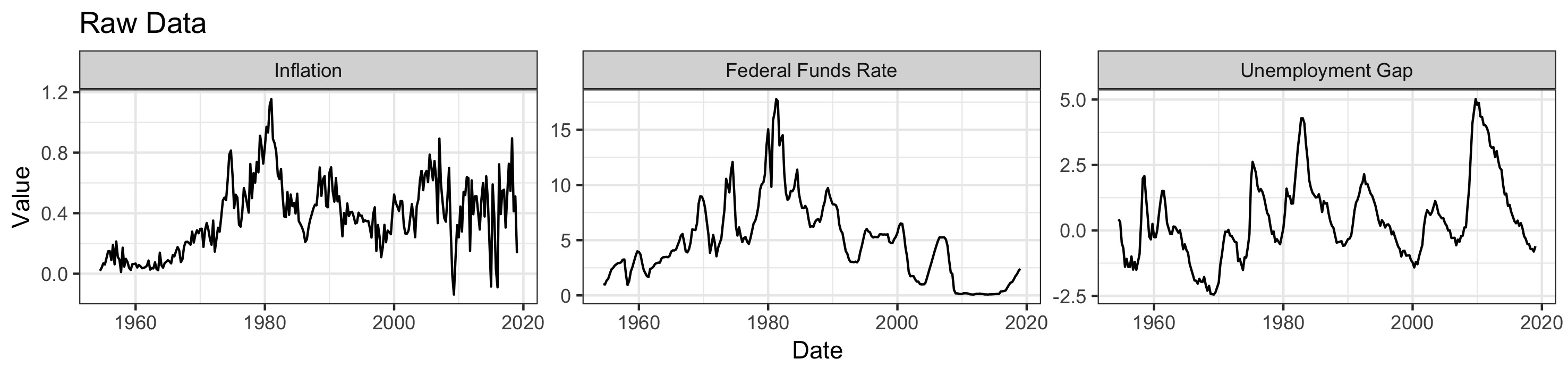
We use the FRED database of the Federal Reserve Bank of St. Louis and retrieve series for the unemployment gap $n_{t}$ , i.e. we subtract the unemployment rate (UNRATE) from the natural unemployment rate (NROU), inflation $\pi_{t}$ (lagged differences of GDPDEF), and the effective federal funds rate $R_{t}$ (FEDFUNDS). The observation period starts with Q3 1954 and ends with Q1 2019, thus there are 259 observations.

5.2.2 Estimation Procedure

In order to select appropriate integer-valued parameters $p$ and $q$ , we estimate a number of VARMA models with the MTS-package and select the one with the smallest AIC value. It is worth noting that neither the dse-package nor the MTS-package enforces the stability condition (2) or the invertibility condition (3). In case of unstable or non-invertible determinantal roots of the $a(z)$ or $b(z)$ matrix polynomials, we mirror these roots outside the unit circle and adjust the error covariance accordingly. Based on the AIC value, the Ljung-Box test, and the McLeod-Li test Mahdi and McLeod 2018, we choose $p=2$ and $q=2$ . Moreover, the distribution of the shocks of the initial model in Figure 2 and Figure 3 suggest, and the Jarque-Bera test indicates that the individual series are not normally distributed.

We proceed thus under the assumption that the errors of the VARMA(2,2) model are independent and not normally distributed. The individual series seem leptokurtic and we assume that they follow a Laplace distribution. The full conditional likelihood is subsequently estimated using the same identification scheme as in Lanne et al. 2017 for fixing a particular permutation and scaling. The estimates for $B$ and $\sigma$ are

\hat{B}=\begin{pmatrix}1&0.1224&-0.1282\\ -0.0168&1&0.0107\\ 0.0280&0.175&1\end{pmatrix}

and $\hat{\sigma}=\left(0.0685,\,0.0315,\,0.14\right)$ , the respective (bootstrapped) standard deviations are

\hat{\mathbb{V}}_{bs}\left(\hat{B}\right)=\begin{pmatrix}0&0.1204&0.01496\\ 0.02816&0&0.0156\\ 0.06903&0.0928&0\end{pmatrix}

and $\hat{\mathbb{V}}_{bs}\left(\hat{\sigma}\right)=\left(0.00427,\,0.00199,\,0.01419\right)$ .

5.2.3 Impulse Response Function

In order to interpret the results, we calculate the impulse response function together with bootstrapped confidence intervals (1000 bootstrap replications).

We interpret the third shock as a (in the longer term) contractionary monetary policy shock since it is the only one to which the interest rate reacts significantly (judging from the confidence bands). In the medium term, the unemployment gap widens (the economy shrinks) and initially there is a positive response of inflation to Shock 3. The first shock is interpreted as negative demand shock because the economy shrinks (widening of the unemployment gap) and prices fall slightly. We interpret the remaining Shock 2 as negative supply shock since the economy shrinks (widening unemployment gap) with increasing prices.

6 Acknowledgements

Financial support by the Research Funds of the University of Helsinki as well as by funds of the Oesterreichische Nationalbank (Austrian Central Bank, Anniversary Fund, project number: 17646) is gratefully acknowledged. For bootstrapping, the Finnish Grid and Cloud Infrastructure with persistent identifier urn:nbn:fi:research-infras-2016072533 was used. Juho Koistinen, Mika Meitz, Markku Lanne, and Wolfgang Scherrer provided helpful comments on various versions of this article.

7 Conclusion

In this article, we showed that stable and invertible SVARMA models (1) driven by independent and non-Gaussian shocks are identifiable up to permutation and scaling. This result extends the identifiability results regarding structural VAR models in Lanne et al. 2017. SVARMA models capture (macroeconomic) dynamics more parsimoniously than SVAR models and are therefore advantageous in situations with relatively small sample sizes.

References

Athanasopoulos and Vahid (2008a) George Athanasopoulos and Farshid Vahid. Varma versus var for macroeconomic forecasting. Journal of Business & Economic Statistics, 26(2):237–252, 2008a. doi: 10.1198/073500107000000313.
Athanasopoulos and Vahid (2008b) George Athanasopoulos and Farshid Vahid. A complete varma modelling methodology based on scalar components. Journal of Time Series Analysis, 29(3):533–554, 2008b. doi: 10.1111/j.1467-9892.2007.00568.x.
Boubacar Mainassara and Francq (2011) Yacouba Boubacar Mainassara and Christian Francq. Estimating structural varma models with uncorrelated but non-independent error terms. Journal of Multivariate Analysis, 102(3):496 – 505, 2011. doi: 10.1016/j.jmva.2010.10.009.
Chen and Bickel (2005) Aiyou Chen and Peter J. Bickel. Consistent independent component analysis and prewhitening. IEEE Transactions on Signal Processing, 53:3625–3632, 2005. doi: 10.1109/TSP.2005.855098.
Deistler (1983) Manfred Deistler. The Properties of the Parameterization of ARMAX Systems and Their Relevance for Structural Estimation and Dynamic Specification. Econometrica, 51(4):1187–1207, July 1983. URL http://www.jstor.org/stable/1912058.
Deistler and Seifert (1978) Manfred Deistler and Hans-Günther Seifert. Identifiability and Consistent Estimability in Econometric Models. Econometrica, 46(6):969–980, July 1978. URL http://www.jstor.org/stable/1909759.
Gilbert (2015) Paul D. Gilbert. dse: Dynamic Systems Estimation (Time Series Package), 2015. URL https://cran.r-project.org/package=dse.
Golub and Van Loan (2013) Gene H. Golub and Charles F. Van Loan. Matrix Computations. The Johns Hopkins University Press, 4th edition, 2013.
Gomez (2015) Victor Gomez. SSMMATLAB: A set of matlab programs for the statistical analysis of state space models. Journal of Statistical Software, 66(9):1–37, 2015. ISSN 1548-7660. doi: 10.18637/jss.v066.i09.
Gomez (2016) Victor Gomez. Multivariate Time Series With Linear State Space Structure. Springer, 2016.
Gourieroux et al. (2017) Christian Gourieroux, Alain Monfort, and Jean-Paul Renne. Statistical inference for independent component analysis: Application to structural VAR models. Journal of Econometrics, 196:111–126, 2017. doi: 10.1016/j.jeconom.2016.09.007.
Gourieroux et al. (2019) Christian Gourieroux, Alain Monfort, and Jean-Paul Renne. Identification and Estimation in Non-Fundamental Structural VARMA Models. Review of Economic Studies, pages 1–39, 2019. doi: 10.193/restud/rdz028.
Hallin and Mehta (2015) Marc Hallin and Chintan Mehta. R-estimation for asymmetric independent component analysis. Journal of the American Statistical Association, 110(509):218–232, 2015. doi: 10.1080/01621459.2014.909316.
Hannan (1970) Edward J. Hannan. Multiple Time Series. Wiley, 1970.
Hannan (1971) Edward J. Hannan. The identification problem for multiple equation systems with moving average errors. Econometrica, 39(5):751–765, September 1971. doi: 10.2307/1909577.
Hannan and Deistler (2012) Edward J. Hannan and Manfred Deistler. The Statistical Theory of Linear Systems. SIAM Classics in Applied Mathematics, Philadelphia, 2012.
Harville (1997) David A. Harville. Matrix Algebra From a Statistician’s Perspective. Springer, 1997.
Ilmonen and Paindaveine (2011) Pauliina Ilmonen and Davy Paindaveine. Semiparametrically efficient inference based on signed ranks in symmetric independent component models. Annals of Statistics, 39(5):2448–2476, 2011. doi: 10.1214/11-AOS906.
Kagan et al. (1973) Abram M. Kagan, Yuri V. Linnik, and Calyampudi R. Rao. Characterization Problems in Mathematical Statistics. John Wiley & Sons, 1973.
Kilian and Lütkepohl (2017) Lutz Kilian and Helmut Lütkepohl. Structural Vector Autoregressive Analysis. Cambridge University Press, 2017. doi: 10.1017/9781108164818.
Lanne et al. (2017) Markku Lanne, Mika Meitz, and Pentti Saikkonen. Identification and estimation of non-gaussian structural vector autoregressions. Journal of Econometrics, 196(2):288 – 304, 2017. doi: 10.1016/j.jeconom.2016.06.002.
Lütkepohl (1996) Helmut Lütkepohl. Handbook of Matrices. John Wiley & Sons Ltd., 1996.
Lütkepohl (2005) Helmut Lütkepohl. New Introduction to Multiple Time Series Analysis. Springer Berlin, 2005.
Magnus and Neudecker (2007) Jan R. Magnus and Heinz Neudecker. Matrix Differential Calculus with Applications in Statistics and Econometrics. John Wiley & Sons, 2007.
Mahdi and McLeod (2018) Esam Mahdi and A. Ian McLeod. portes: Portmanteau Tests for Univariate and Multivariate Time Series Models, 2018. R package version 3.0.
Meitz and Saikkonen (2013) Mika Meitz and Pentti Saikkonen. Maximum likelihood estimation of a noninvertible arma model with autoregressive conditional heteroskedasticity. Journal of Multivariate Analysis, 114:227 – 255, 2013. doi: 10.1016/j.jmva.2012.07.015.
Poskitt (2016) Donald S. Poskitt. Vector autoregressive moving average identification for macroeconomic modeling: A new methodology. Journal of Econometrics, 192:468–484, June 2016. doi: 10.1016/j.jeconom.2016.02.011.
Poskitt and Yao (2017) Donald S. Poskitt and Wenying Yao. Vector autoregressions and macroeconomic modeling: An error taxonomy. Journal of Business & Economic Statistics, 35(3):407–419, 2017. doi: 10.1080/07350015.2015.1077139.
Pötscher and Prucha (1997) Benedikt Pötscher and Ingmar Prucha. Dynamic Nonlinear Econometric Models, Asymptotic Theory. Springer Berlin, 1997.
R Core Team (2019) R Core Team. R: A Language and Environment for Statistical Computing. R Foundation for Statistical Computing, Vienna, Austria, 2019. URL https://www.R-project.org/.
Raghavan et al. (2016) Mala Raghavan, George Athanasopoulos, and Param Silvapulle. Canadian monetary policy analysis using a structural varma model. Canadian Journal of Economics, 49(1):347–373, 2016. doi: 10.1111/caje.12200.
Ravenna (2007) Federico Ravenna. Vector autoregressions and reduced form representations of {DSGE} models. Journal of Monetary Economics, 54(7):2048 – 2064, 2007. ISSN 0304-3932. doi: 10.1016/j.jmoneco.2006.09.002.
Rothenberg (1971) Thomas J. Rothenberg. Identification in Parametric Models. Econometric Theory, 39(3):577–591, May 1971. doi: 10.2307/1913267.
Scherrer and Deistler (2019) Wolfgang Scherrer and Manfred Deistler. Vector autoregressive moving average models. In Hrishikesh D. Vinod and C. R. Rao, editors, Handbook of statistics 41, volume 41. North-Holland, 2019.
Scherrer and Funovits (2019) Wolfgang Scherrer and Bernd Funovits. rldm: A package for modeling of time series with a rational spectral density, 2019.
Seber (2008) George A. F. Seber. A Matrix Handbook for Statisticians. John Wiley & Sons, 2008.
Tsay (2013) Ruey S. Tsay. Multivariate Time Series Analysis With R and Financial Applications. John Wiley & Sons, Inc., Hoboken, New Jersey, 2013.
Tsay and Wood (2018) Ruey S. Tsay and David Wood. MTS: All-Purpose Toolkit for Analyzing Multivariate Time Series (MTS) and Estimating Multivariate Volatility Models, 2018. R package version 1.0.

Appendix A Introduction to the Online Appendix

We obtain the first and second partial derivatives of the individual contributions $l_{t}(\theta)$ to the standardized log-likelihood function $L_{T}\left(\theta\right)$ and show that Assumptions 2 to 5 imply that the premises of Theorem 2 are satisfied. The rest of this Online Appendix is structured as follows.

After introducing some notation in the rest of this section, we calculate the first partial derivatives of $l_{t}(\theta)$ in Section B. In Section C we show that the first partial derivatives of $l_{t}(\theta)$ are an MDS. In Section D we derive the expression for the expectation of the outer product of the score at the true parameter value $\theta_{0}$ and in Section E we verify that it is finite. This verifies that the score satisfies a CLT for MDS.

In Section F we derive the matrix of second partial derivatives of $l_{t}\left(\theta\right)$ while in Section G we verify that the expectation of the supremum (over a compact and convex set in the parameter space which contains the true parameter value) of the Hessian is finite. This verifies that the Hessian satisfies a ULLN.

In Section H it is verified that the expectation of the Hessian equals the expectation of the outer product of the score, evaluated respectively at the true parameter value $\theta_{0}$ . Together with the above, all statements in Theorem 2 are verified.

A.1 Notation and System Representations

The individual contribution at time $t$ to the (standardized) log-likelihood function, i.e. equation (7), is here repeated as

l_{t}\left(\theta\right)=\sum_{i=1}^{n}\log\left[f_{i}\left(\sigma_{i}^{-1}\varepsilon_{i,t}\left(\theta\right);\lambda_{i}\right)\right]-\log\left\{\det\left[B\left(\beta\right)\right]\right\}-\sum_{i=1}^{n}\log\left(\sigma_{i}\right),

where $\varepsilon_{i,t}\left(\theta\right)=\iota_{i}^{{}^{\prime}}B\left(\beta\right)^{-1}u_{t}\left(\theta\right).$

Derivatives of the component densities.

For the first partial derivatives of $l_{t}\left(\theta\right)$ , the expressions

e_{i,x,t}(\theta)=\frac{\partial}{\partial x}\log\left[f_{i}\left(\sigma_{i}^{-1}\iota_{i}^{\prime}B\left(\beta\right)^{-1}u_{t}\left(\theta\right);\lambda_{i}\right)\right]=\frac{f_{i,x}\left(\sigma_{i}^{-1}\iota_{i}^{\prime}B\left(\beta\right)^{-1}u_{t}\left(\theta\right);\lambda_{i}\right)}{f_{i}\left(\sigma_{i}^{-1}\iota_{i}^{\prime}B^{\prime}\left(\beta\right)^{-1}u_{t}\left(\theta\right);\lambda_{i}\right)}

and

e_{i,\lambda_{i},t}(\theta)=\frac{\partial}{\partial\lambda_{i}}\log\left[f_{i}\left(\sigma_{i}^{-1}\iota_{i}^{\prime}B\left(\beta\right)^{-1}u_{t}\left(\theta\right);\lambda_{i}\right)\right]=\frac{f_{i,\lambda}\left(\sigma_{i}^{-1}\iota_{i}^{\prime}B\left(\beta\right)^{-1}u_{t}\left(\theta\right);\lambda_{i}\right)}{f_{i}\left(\sigma_{i}^{-1}\iota_{i}^{\prime}B\left(\beta\right)^{-1}u_{t}\left(\theta\right);\lambda_{i}\right)},

where $f_{i,x}\left(x;\lambda_{i}\right)=\frac{\partial}{\partial x}f_{i}\left(x;\lambda_{i}\right)$ and $f_{i,\lambda_{i}}\left(x;\lambda_{i}\right)=\frac{\partial}{\partial\lambda_{i}}f_{i}\left(x;\lambda_{i}\right)$ will be used extensively. The corresponding versions for all components are $e_{x,t}\left(\theta\right)=\left(e_{1,x,t}\left(\theta\right),\ldots,e_{n,x,t}\left(\theta\right)\right)^{\prime}$ of dimension $n$ and $e_{\lambda,t}\left(\theta\right)=\left(e_{1,\lambda_{1},t}^{\prime}\left(\theta\right),\ldots,e_{n,\lambda_{n},t}^{\prime}\left(\theta\right)\right)^{\prime}$ of dimension $d=d_{1}+\cdots+d_{n}$ .

For the second partial derivatives of $l_{t}\left(\theta\right)$ , the expressions

e_{i,xx,t}\left(\theta\right)=\frac{\partial e_{i,x,t}\left(\theta\right)}{\partial x}=\left(\frac{f_{i,xx}f_{i}-f_{i,x}^{2}}{f_{i}^{2}}\right)\left(\sigma_{i}^{-1}\iota_{i}^{\prime}B\left(\beta\right)^{-1}u_{t}\left(\theta\right);\lambda_{i}\right),

e_{i,x\lambda_{i},t}\left(\theta\right)=\frac{\partial e_{i,x,t}\left(\theta\right)}{\partial\lambda_{i}}=\left(\frac{f_{i,x\lambda}f_{i}-f_{i,\lambda_{i}}f_{i,x}^{2}}{f_{i}^{2}}\right)\left(\sigma_{i}^{-1}\iota_{i}^{\prime}B\left(\beta\right)^{-1}u_{t}\left(\theta\right);\lambda_{i}\right),

and

e_{i,\lambda_{i}\lambda_{i},t}(\theta)=\frac{\partial e_{i,\lambda_{i},t}(\theta)}{\partial\lambda_{i}^{\prime}}=\left(\frac{f_{i,\lambda_{i}\lambda_{i}}f_{i}-f_{i,\lambda_{i}}f_{i,\lambda_{i}}^{\prime}}{f_{i}^{2}}\right)\left(\sigma_{i}^{-1}\iota_{i}^{\prime}B\left(\beta\right)^{-1}u_{t}\left(\theta\right);\lambda_{i}\right),

are important. Here, $e_{xx,t}\left(\theta\right)=diag\left(e_{1,xx,t}\left(\theta\right),\ldots,e_{n,xx,t}\left(\theta\right)\right)$ is a diagonal matrix of dimension $n$ and $e_{\lambda\lambda,t}(\theta)=diag\left(e_{1,\lambda_{1}\lambda_{1},t}(\theta),\ldots,e_{n,\lambda_{n}\lambda_{n},t}(\theta)\right)$ is a block diagonal matrix with blocks of size $d_{i}$ . The notation $\frac{\partial e_{i,x,t}\left(\theta_{0}\right)}{\partial x}:=\left.\frac{\partial e_{i,x,t}\left(\theta\right)}{\partial x}\right|_{\theta=\theta_{0}}$ is used to denote the derivative evaluated at a particular point.

Two different ways to express the partial derivatives of $u_{t}\left(\theta\right)$ .

The observations may be represented at one particular point in time or as a system containing all observations $\left(y_{1},\ldots,y_{T}\right)$ as well as starting values $\left(y_{1-p},\ldots,y_{0}\right)$ . The starting values for the process $\left(u_{t}\right)$ are set to zero, i.e. $\left(u_{1-q},\ldots,u_{0}\right)=0$ . For simplicity, we also set the starting values $\left(y_{1-p},\ldots,y_{0}\right)$ equal to zero. If clarity of presentation is not affected, we use $x_{t-1}=\left(y^{\prime}_{t-1},\ldots,y^{\prime}_{t-p}\right)^{{}^{\prime}}$ of dimension $np$ and $w_{t-1}\left(\theta\right)=\left(u^{\prime}_{t-1}\left(\theta\right),\ldots,u^{\prime}_{t-q}\left(\theta\right)\right)^{{}^{\prime}}$ of dimension $nq$ as shorthand notation.

For one particular point in time, we have

u_{t}\left(\theta\right)=y_{t}-\left(a_{1},\ldots,a_{p}\right)\begin{pmatrix}y_{t-1}\\ \vdots\\ y_{t-p}\end{pmatrix}-\left(b_{1},\ldots,b_{q}\right)\begin{pmatrix}u_{t-1}\left(\theta\right)\\ \vdots\\ u_{t-q}\left(\theta\right)\end{pmatrix}

(8)

for $t\in\left\{1,\ldots,T\right\}$ .

All observations can be written as

\left(y_{1}\cdots y_{T}\right)-a_{1}\left(y_{0}\cdots y_{T-1}\right)-\cdots-a_{p}\left(y_{1-p}\cdots y_{T-p}\right)=\left(u_{1}\left(\theta\right)\cdots u_{T}\left(\theta\right)\right)+b_{1}+\cdots+b_{q}\left(u_{1-q}\left(\theta\right)\cdots u_{T-q}\left(\theta\right)\right).

(9)

Defining the matrix

L=\begin{pmatrix}0&\cdots&&\cdots&0\\ 1&0&\cdots&&\vdots\\ 0&1&0\\ \vdots&\ddots&\ddots&\ddots&\vdots\\ 0&\cdots&0&1&0\end{pmatrix}\in\mathbb{R}^{T\times T}

corresponding to the (non-invertible) lag operator such that

L\begin{pmatrix}u_{1}^{\prime}\left(\theta\right)\\ u_{2}^{\prime}\left(\theta\right)\\ \vdots\\ u_{T}^{\prime}\left(\theta\right)\end{pmatrix}=\begin{pmatrix}0_{1\times n}\\ u_{1}^{\prime}\left(\theta\right)\\ \vdots\\ u_{T-1}^{\prime}\left(\theta\right)\end{pmatrix},

equation (9) can be written as

\left(y_{1}\cdots y_{T}\right)-a_{1}\left(y_{0}\cdots y_{T-1}\right)-\cdots-a_{p}\left(y_{1-p}\cdots y_{T-p}\right)=\left(u_{1}\left(\theta\right)\cdots u_{T}\left(\theta\right)\right)+b_{1}\left(u_{1}\left(\theta\right)\cdots u_{T}\left(\theta\right)\right)L^{\prime}+\cdots+b_{q}\left(u_{1}\left(\theta\right)\cdots u_{T}\left(\theta\right)\right)\left(L^{\prime}\right)^{q}.

Vectorizing equation (9) leads to

	$\displaystyle vec\left(y_{1}\cdots y_{T}\right)-\left[\begin{pmatrix}y_{0}^{\prime}\\ y_{1}^{\prime}\\ \vdots\\ y_{T-1}^{\prime}\end{pmatrix}\otimes I_{n},\begin{pmatrix}y_{-1}^{\prime}\\ y_{0}^{\prime}\\ \vdots\\ y_{T-2}^{\prime}\end{pmatrix}\otimes I_{n},\ldots,\begin{pmatrix}y_{1-p}^{\prime}\\ y_{2-p}^{\prime}\\ \vdots\\ y_{T-p}^{\prime}\end{pmatrix}\otimes I_{n}\right]\underbrace{vec\left(a_{1},\ldots,a_{p}\right)}_{=\pi_{2}}=$		(10)
	$\displaystyle=vec\left(u_{1}\left(\theta\right)\cdots u_{T}\left(\theta\right)\right)+\left[L\begin{pmatrix}u_{1}^{\prime}\left(\theta\right)\\ u_{2}^{\prime}\left(\theta\right)\\ \vdots\\ u_{T}^{\prime}\left(\theta\right)\end{pmatrix}\otimes I_{n},L^{2}\begin{pmatrix}u_{1}^{\prime}\left(\theta\right)\\ u_{2}^{\prime}\left(\theta\right)\\ \vdots\\ u_{T}^{\prime}\left(\theta\right)\end{pmatrix}\otimes I_{n},\ldots,L^{q}\begin{pmatrix}u_{1}^{\prime}\left(\theta\right)\\ u_{2}^{\prime}\left(\theta\right)\\ \vdots\\ u_{T}^{\prime}\left(\theta\right)\end{pmatrix}\otimes I_{n}\right]\underbrace{vec\left(b_{1},\ldots,b_{p}\right)}_{=\pi_{3}}$
	$\displaystyle=\left[I_{Tn}+\sum_{i=1}^{q}\left(L^{i}\otimes b_{i}\right)\right]vec\left(u_{1}\left(\theta\right)\cdots u_{T}\left(\theta\right)\right)$

where the vectorization formula $vec\left(ABC\right)=\left(C^{\prime}\otimes A\right)vec(B)$ has been applied to $\left\{\left[I_{n}\right]\left[a_{j}\right]\left[\left(y_{1-j}\cdots y_{T-j}\right)\right]\right\}$ on the left-hand-side and to $\left(\left[b_{j}\right]\left[\left(u_{1}\left(\theta\right)\cdots u_{T}\left(\theta\right)\right)\right]\left[\left(L^{\prime}\right)^{j}\right]\right)$ and $\left(\left[I_{n}\right]\left[b_{j}\right]\left[\left(u_{1}\left(\theta\right)\cdots u_{T}\left(\theta\right)\right)\left(L^{\prime}\right)^{j}\right]\right)$ on the right-hand-side of equation (9)

By using the (conditional maximum likelihood) assumption that $\left(y_{1-p},\ldots,y_{0}\right)$ be zero, we can also vectorize the left-hand-side of equation (9) as

vec\left[\left(y_{1}\cdots y_{T}\right)-a_{1}\left(y_{1}\cdots y_{T}\right)L^{\prime}-\cdots-a_{p}\left(y_{1}\cdots y_{T}\right)\left(L^{\prime}\right)^{p}\right]=vec\left(y_{1}\cdots y_{T}\right)-\sum_{j=1}^{p}\left(L^{j}\otimes a_{j}\right)vec\left(y_{1}\cdots y_{T}\right)

in order to obtain

\mathcal{B}\begin{pmatrix}u_{1}\left(\theta\right)\\ \vdots\\ u_{T}\left(\theta\right)\end{pmatrix}=\mathcal{A}\begin{pmatrix}y_{1}\\ \vdots\\ y_{T}\end{pmatrix}

where

\mathcal{A}=\left[I_{Tn}-\sum_{i=1}^{p}\left(L^{i}\otimes a_{i}\right)\right]=\begin{pmatrix}I_{n}&0&&\cdots&0&\cdots&&0\\ -a_{1}&I_{n}&0&&&&&\vdots\\ -a_{2}&-a_{1}&I_{n}&\ddots&&&&0\\ \vdots&-a_{2}&\ddots&\ddots&0&&&0\\ -a_{p}&&\ddots&-a_{1}&I_{n}&\ddots&&\vdots\\ 0&-a_{p}&&&\ddots&\ddots&0&0\\ \vdots&0&\ddots&&-a_{2}&-a_{1}&I_{n}&0\\ 0&\cdots&0&-a_{p}&\cdots&-a_{2}&-a_{1}&I_{n}\end{pmatrix}\in\mathbb{R}^{Tn\times Tn}

and

\mathcal{B}=\left[I_{Tn}+\sum_{i=1}^{q}\left(L^{i}\otimes b_{i}\right)\right]=\begin{pmatrix}I_{n}&0&&\cdots&0&\cdots&&0\\ b_{1}&I_{n}&0&&&&&\vdots\\ b_{2}&b_{1}&I_{n}&\ddots&&&&0\\ \vdots&b_{2}&\ddots&\ddots&0&&&0\\ b_{q}&&\ddots&b_{1}&I_{n}&\ddots&&\vdots\\ 0&b_{q}&&&\ddots&\ddots&0&0\\ \vdots&0&\ddots&&b_{2}&b_{1}&I_{n}&0\\ 0&\cdots&0&b_{q}&\cdots&b_{2}&b_{1}&I_{n}\end{pmatrix}\in\mathbb{R}^{Tn\times Tn}.

Appendix B Partial Derivatives of $l_{t}\left(\theta\right)$

In the following subsections, we will derive that

	$\displaystyle\frac{\partial l_{t}\left(\theta_{0}\right)}{\partial\pi_{2}}$	$\displaystyle=-x_{b,t-1}\left(\theta_{0}\right)B^{\prime}\left(\beta_{0}\right)^{-1}\Sigma_{0}^{-1}e_{x,t}\left(\theta_{0}\right)$
	$\displaystyle\frac{\partial l_{t}\left(\theta_{0}\right)}{\partial\pi_{3}}$	$\displaystyle=-w_{b,t-1}\left(\theta_{0}\right)\Sigma_{0}^{-1}e_{x,t}\left(\theta_{0}\right)$
	$\displaystyle\frac{\partial l_{t}\left(\theta_{0}\right)}{\partial\beta}$	$\displaystyle=H^{\prime}\sum_{i=1}^{q}\left(I_{n}\otimes b_{i}^{\prime}B^{\prime}\left(\beta_{0}\right)^{-1}\Sigma_{0}^{-1}\right)\left(\varepsilon_{t-i}\left(\theta_{0}\right)\otimes e_{x,t}\left(\theta_{0}\right)\right)-H^{\prime}\left(I_{n}\otimes B^{\prime}\left(\beta_{0}\right)^{-1}\Sigma_{0}^{-1}\right)\left(\varepsilon_{t}\left(\theta_{0}\right)\otimes e_{x,t}\left(\theta_{0}\right)\right)-H^{\prime}vec\left(B^{\prime}\left(\beta_{0}\right)^{-1}\right)$
	$\displaystyle\frac{\partial}{\partial\sigma}l_{t}\left(\theta_{0}\right)$	$\displaystyle=-\Sigma_{0}^{-2}\left[e_{x,t}\left(\theta_{0}\right)\odot\varepsilon_{t}\left(\theta_{0}\right)+\sigma_{0}\right]$
	$\displaystyle\frac{\partial}{\partial\lambda}l_{t}\left(\theta_{0}\right)$	$\displaystyle=e_{\lambda,t}\left(\theta_{0}\right)$

B.1 Partial Derivative with respect to $\pi_{2}$

Intermediate step for $l_{\pi_{2},t}\left(\theta\right)$ .

We obtain that

$\displaystyle\frac{\partial l_{t}\left(\theta\right)}{\partial\pi_{2}}$	$\displaystyle=\frac{\partial}{\partial\pi_{2}}\left\{\sum_{i=1}^{n}\log\left[f_{i}\left(\sigma_{i}^{-1}\iota_{i}^{{}^{\prime}}B\left(\beta\right)^{-1}u_{t}\left(\theta\right);\lambda_{i}\right)\right]\right\}=\frac{\partial}{\partial\pi_{2}}\left\{\sum_{i=1}^{n}\log\left[f_{i}\left(\sigma_{i}^{-1}u_{t}\left(\theta\right)^{\prime}B^{\prime}\left(\beta\right)^{-1}\iota_{i};\lambda_{i}\right)\right]\right\}$
	$\displaystyle=\sum_{i=1}^{n}e_{i,x,t}\left(\theta\right)\frac{\partial u_{t}\left(\theta\right)^{\prime}}{\partial\pi_{2}}\sigma_{i}^{-1}B^{\prime}\left(\beta\right)^{-1}\iota_{i}$
	$\displaystyle=\frac{\partial u_{t}\left(\theta\right)^{\prime}}{\partial\pi_{2}}B^{\prime}\left(\beta\right)^{-1}\Sigma^{-1}e_{x,t}$	(11)

The derivative of $u_{t}$ with respect to $\pi_{2}$ for one equation.

We obtain from vectorizing (8) that

	$\displaystyle u_{t}\left(\theta\right)$	$\displaystyle=y_{t}-\left(a_{1},\ldots,a_{p}\right)\begin{pmatrix}y_{t-1}\\ \vdots\\ y_{t-p}\end{pmatrix}-\left(b_{1},\ldots,b_{q}\right)\begin{pmatrix}u_{t-1}\left(\theta\right)\\ \vdots\\ u_{t-q}\left(\theta\right)\end{pmatrix}$
		$\displaystyle=y_{t}-\left(\left(y^{\prime}_{t-1},\ldots,y^{\prime}_{t-p}\right)\otimes I_{n}\right)vec\left(a_{1},\ldots,a_{p}\right)-\left(b_{1},\ldots,b_{q}\right)\begin{pmatrix}u_{t-1}\left(\theta\right)\\ \vdots\\ u_{t-q}\left(\theta\right)\end{pmatrix}.$

Transposition and differentiation lead to

u_{t}^{\prime}\left(\theta\right)=y_{t}^{\prime}-\pi_{2}^{\prime}\left(\begin{pmatrix}y_{t-1}\\ \vdots\\ y_{t-p}\end{pmatrix}\otimes I_{n}\right)-\left(u_{t-1}^{\prime}\left(\theta\right),\ldots,u_{t-q}^{\prime}\left(\theta\right)\right)\begin{pmatrix}b_{1}^{\prime}\\ \vdots\\ b_{q}^{\prime}\end{pmatrix}

and

\frac{\partial u_{t}^{\prime}\left(\theta\right)}{\partial\pi_{2}}=-\left(x_{t-1}\otimes I_{n}\right)-\left(\frac{\partial u_{t-1}^{\prime}\left(\theta\right)}{\partial\pi_{2}},\ldots,\frac{\partial u_{t-q}^{\prime}\left(\theta\right)}{\partial\pi_{2}}\right)\begin{pmatrix}b_{1}^{\prime}\\ \vdots\\ b_{q}^{\prime}\end{pmatrix}.

Finally, we may express $\frac{\partial u_{t}\left(\theta\right)}{\partial\pi_{2}^{\prime}}$ using a lag polynomial, i.e.

	$\displaystyle\left(I_{n}+b_{1}z+\cdots+b_{q}z^{q}\right)\overbrace{\frac{\partial u_{t}\left(\theta\right)}{\partial\pi_{2}^{\prime}}}^{n\times n^{2}p}$	$\displaystyle=-\overbrace{\left(x_{t-1}^{\prime}\otimes I_{n}\right)}^{=\left(n\times n^{2}p\right)}$
	$\displaystyle\iff\frac{\partial u_{t}\left(\theta\right)}{\partial\pi_{2}^{\prime}}$	$\displaystyle=-b(z)^{-1}\left[x_{t-1}^{\prime}\otimes I_{n}\right]=-\left[x_{t-1}^{\prime}\otimes b(z)^{-1}\right].$

The derivative of $u_{t}$ with respect to $\pi_{2}$ for all points in time.

Rewriting equation (10) as

\displaystyle\begin{pmatrix}y_{1}\\ \vdots\\ y_{T}\end{pmatrix}-\left[\begin{pmatrix}x_{0}^{\prime}\\ \vdots\\ x_{T-1}^{\prime}\end{pmatrix}\otimes I_{n}\right]\underbrace{vec\left(a_{1},\ldots,a_{p}\right)}_{=\pi_{2}}

\displaystyle=\underbrace{\left[I_{Tn}-\sum_{i=1}^{q}\left(L^{i}\otimes b_{i}\right)\right]}_{=\mathcal{B}}vec\left(u_{1}\left(\theta\right)\cdots u_{T}\left(\theta\right)\right),

transposing it and taking partial derivatives leads to

	$\displaystyle\frac{\partial}{\partial\pi_{2}}\begin{pmatrix}u^{\prime}_{1}\left(\theta\right)&\cdots&u^{\prime}_{T}\left(\theta\right)\end{pmatrix}$	$\displaystyle=-\frac{\partial}{\partial\pi_{2}}\left[\pi^{\prime}_{2}\left[\begin{pmatrix}x_{0}&\cdots&x_{T-1}\end{pmatrix}\otimes I_{n}\right]\mathcal{B}^{\prime-1}\right]$
		$\displaystyle=-\left[\begin{pmatrix}x_{0}&\cdots&x_{T-1}\end{pmatrix}\otimes I_{n}\right]\mathcal{B}^{\prime-1}.$

It follows that for one point in time, we obtain over a compact set centered at the true parameter value is finite

\frac{\partial u^{\prime}_{t}\left(\theta\right)}{\partial\pi_{2}}=-\left[\begin{pmatrix}x_{0}&\cdots&x_{T-1}\end{pmatrix}\otimes I_{n}\right]\underbrace{\left(\mathcal{B}^{\prime-1}\right)_{\left[\bullet,t\right]}}_{=\mathfrak{b_{t}}}

where $\mathfrak{b}_{t}=\left(\mathcal{B}^{\prime-1}\right)_{\left[\bullet,t\right]}$ is the $t$ -th $\left(Tn\times n\right)$ -dimensional block of columns of the $\left(Tn\times Tn\right)$ -dimensional matrix $\mathcal{B}^{\prime-1}$ . Note that $\mathcal{B}^{\prime-1}$ is (block-) upper-triangular such that the product of $\left[\begin{pmatrix}x_{0}&\cdots&x_{T-1}\end{pmatrix}\otimes I_{n}\right]$ with $\mathfrak{b}_{t}$ only involves terms depending on time $t-1$ and earlier. Furthermore, note that the non-zero elements of $\mathfrak{b}_{t}$ correspond to the coefficients of $b(z)^{-1}$ whose (matrix-) norms are decreasing at an exponential rate.

Result for $l_{\pi_{2},t}\left(\theta\right)$ for one point in time.

In the expression involving $\left[x_{t.-1}\otimes b^{\prime}(z)^{-1}\right]$ below, it is unclear to which quantity the lag operator applies. This is why we introduce addional notation $x_{t-1}\otimes b^{\prime}(z)^{-1}=x_{b,t-1}\left(\theta\right)$ in a similar way as in Meitz and Saikkonen 2013.

This implies for the score that

	$\displaystyle\frac{\partial l_{t}\left(\theta\right)}{\partial\pi_{2}}$	$\displaystyle=-\left[\begin{pmatrix}x_{0}&\cdots&x_{T-1}\end{pmatrix}\otimes I_{n}\right]\mathfrak{b}_{t}B^{\prime}\left(\beta\right)^{-1}\Sigma^{-1}e_{x,t}\left(\theta\right)$
		$\displaystyle=-\left[x_{t.-1}\otimes b^{\prime}(z)^{-1}\right]B^{\prime}\left(\beta\right)^{-1}\Sigma^{-1}e_{x,t}\left(\theta\right)$
		$\displaystyle=-x_{b,t-1}\left(\theta\right)B^{\prime}\left(\beta\right)^{-1}\Sigma^{-1}e_{x,t}\left(\theta\right).$

Result for $\frac{\partial L_{t}\left(\theta\right)}{\partial\pi_{2}}$ .

The partial derivative of the standardized log-likelihood function with respect to $\pi_{2}$ is

	$\displaystyle\frac{\partial L_{t}\left(\theta\right)}{\partial\pi_{2}}$	$\displaystyle=\frac{1}{T}\sum_{i=1}^{T}l_{\pi_{2},t}\left(\theta\right)$
		$\displaystyle=-\frac{1}{T}\left[\begin{pmatrix}x_{0}&\cdots&x_{T-1}\end{pmatrix}\otimes I_{n}\right]\mathcal{B}^{\prime-1}\left[\left(I_{T}\otimes\Sigma^{-1}B^{\prime}\left(\beta\right)^{-1}\right)\begin{pmatrix}e_{x,1}\left(\theta\right)\\ \vdots\\ e_{x,T}\left(\theta\right)\end{pmatrix}\right].$

B.2 Partial Derivative with respect to $\pi_{3}$

Intermediate step for $l_{\pi_{3},t}\left(\theta\right)$ .

As for (11), we obtain

	$\displaystyle\frac{\partial l_{t}\left(\theta\right)}{\partial\pi_{3}}$	$\displaystyle=\sum_{i=1}^{n}e_{i,x,t}\left(\theta\right)\frac{\partial u_{t}\left(\theta\right)^{\prime}}{\partial\pi_{3}}\sigma_{i}^{-1}B^{\prime}\left(\beta\right)^{-1}\iota_{i}$
		$\displaystyle=\frac{\partial u_{t}\left(\theta\right)^{\prime}}{\partial\pi_{3}}B^{\prime}\left(\beta\right)^{-1}\Sigma^{-1}e_{x,t}\left(\theta\right)$

Applying the product rule to $\frac{\partial u_{t}\left(\theta\right)^{\prime}}{\partial\pi_{3}}$ .

Note that both $\left(b_{1},\ldots,b_{q}\right)$ and $u_{t-j}\left(\theta\right)=B\left(\beta\right)\varepsilon_{t-j}\left(\theta\right)$ depend on $\pi_{3}$ and that the last term in

u_{t}\left(\theta\right)=y_{t}-\left(a_{1},\ldots,a_{p}\right)\begin{pmatrix}y_{t-1}\\ \vdots\\ y_{t-p}\end{pmatrix}-\left(b_{1},\ldots,b_{q}\right)\begin{pmatrix}u_{t-1}\left(\theta\right)\\ \vdots\\ u_{t-q}\left(\theta\right)\end{pmatrix},

can be written as $vec\left[I_{n}\left(b_{1},\ldots,b_{q}\right)\begin{pmatrix}u_{t-1}\left(\theta\right)\\ \vdots\\ u_{t-q}\left(\theta\right)\end{pmatrix}\right]=\left[w_{t-1}^{\prime}\left(\theta\right)\otimes I_{n}\right]\pi_{3}$ . Thus, we obtain that

\frac{\partial u_{t}^{\prime}\left(\theta\right)}{\partial\pi_{3}}=-\left[w_{t-1}\left(\theta\right)\otimes I_{n}\right]-\left[\begin{pmatrix}\frac{\partial u_{t-1}^{\prime}\left(\theta\right)}{\partial\pi_{3}}&\cdots&\frac{\partial u_{t-q}^{\prime}\left(\theta\right)}{\partial\pi_{3}}\end{pmatrix}\begin{pmatrix}b_{1}^{\prime}\\ \vdots\\ b_{q}^{\prime}\end{pmatrix}\right].

Transposing this equation and using the lag operator to solve this equation leads to

	$\displaystyle\left(I_{n}+b_{1}z+\cdots+b_{q}z^{q}\right)\frac{\partial u_{t}\left(\theta\right)}{\partial\pi_{3}^{\prime}}$	$\displaystyle=-\left[w_{t-1}^{\prime}\left(\theta\right)\otimes I_{n}\right]$
	$\displaystyle\iff\frac{\partial u_{t}\left(\theta\right)}{\partial\pi_{3}^{\prime}}$	$\displaystyle=-b(z)^{-1}\left[w_{t-1}^{\prime}\left(\theta\right)\otimes I_{n}\right].$

Applying the product rule to $\frac{\partial\left(u_{1}^{\prime}\left(\theta\right),\ldots,u_{T}^{\prime}\left(\theta\right)\right)}{\partial\pi_{3}}$ .

Rewriting equation (10) as

	$\displaystyle\begin{pmatrix}u_{1}\left(\theta\right)\\ \vdots\\ u_{T}\left(\theta\right)\end{pmatrix}$	$\displaystyle=-\left[\sum_{i=1}^{q}\left(L^{i}\otimes b_{i}\right)\right]\begin{pmatrix}u_{1}\left(\theta\right)\\ \vdots\\ u_{T}\left(\theta\right)\end{pmatrix}+\mathcal{A}\begin{pmatrix}y_{1}\\ \vdots\\ y_{T}\end{pmatrix}+\delta$
		$\displaystyle=-\left[L\begin{pmatrix}u_{1}^{\prime}\left(\theta\right)\\ u_{2}^{\prime}\left(\theta\right)\\ \vdots\\ u_{T}^{\prime}\left(\theta\right)\end{pmatrix}\otimes I_{n},L^{2}\begin{pmatrix}u_{1}^{\prime}\left(\theta\right)\\ u_{2}^{\prime}\left(\theta\right)\\ \vdots\\ u_{T}^{\prime}\left(\theta\right)\end{pmatrix}\otimes I_{n},\ldots,L^{q}\begin{pmatrix}u_{1}^{\prime}\left(\theta\right)\\ u_{2}^{\prime}\left(\theta\right)\\ \vdots\\ u_{T}^{\prime}\left(\theta\right)\end{pmatrix}\otimes I_{n}\right]\pi_{2}+\mathcal{A}\begin{pmatrix}y_{1}\\ \vdots\\ y_{T}\end{pmatrix}+\delta,$
		$\displaystyle=-\left[\begin{pmatrix}u_{0}^{\prime}\left(\theta\right)&\cdots&u_{1-q}^{\prime}\left(\theta\right)\\ \vdots&&\vdots\\ u_{T-1}^{\prime}\left(\theta\right)&\cdots&u_{T-q}^{\prime}\left(\theta\right)\end{pmatrix}\otimes I_{n}\right]\pi_{2}+\mathcal{A}\begin{pmatrix}y_{1}\\ \vdots\\ y_{T}\end{pmatrix}+\delta,$

transposing and taking derivatives leads to

	$\displaystyle\frac{\partial\left(u_{1}^{\prime}\left(\theta\right),\ldots,u_{T}^{\prime}\left(\theta\right)\right)}{\partial\pi_{3}}=-\frac{\partial\left(u_{1}^{\prime}\left(\theta\right),\ldots,u_{T}^{\prime}\left(\theta\right)\right)}{\partial\pi_{3}}\left[\sum_{i=1}^{q}\left(\left(L^{\prime}\right)^{i}\otimes b_{i}^{\prime}\right)\right]-\left[\begin{pmatrix}u_{0}\left(\theta\right)&\cdots&u_{T-1}\left(\theta\right)\\ \vdots&&\vdots\\ u_{1-q}\left(\theta\right)&\cdots&u_{T-q}\left(\theta\right)\end{pmatrix}\otimes I_{n}\right]$
	$\displaystyle\iff\frac{\partial\left(u_{1}^{\prime}\left(\theta\right),\ldots,u_{T}^{\prime}\left(\theta\right)\right)}{\partial\pi_{3}}\underbrace{\left[I_{Tn}+\sum_{i=1}^{q}\left(\left(L^{\prime}\right)^{i}\otimes b_{i}^{\prime}\right)\right]}_{=\mathcal{B}^{\prime}}=-\left[\begin{pmatrix}u_{0}\left(\theta\right)&\cdots&u_{T-1}\left(\theta\right)\\ \vdots&&\vdots\\ u_{1-q}\left(\theta\right)&\cdots&u_{T-q}\left(\theta\right)\end{pmatrix}\otimes I_{n}\right]$

which in turn is equivalent to

	$\displaystyle\frac{\partial\left(u_{1}^{\prime}\left(\theta\right),\ldots,u_{T}^{\prime}\left(\theta\right)\right)}{\partial\pi_{3}}$	$\displaystyle=-\begin{pmatrix}\begin{pmatrix}u_{1}\left(\theta\right)&\cdots&u_{T}\left(\theta\right)\end{pmatrix}L^{\prime}\otimes I_{n}\\ \vdots\\ \begin{pmatrix}u_{1}\left(\theta\right)&\cdots&u_{T}\left(\theta\right)\end{pmatrix}\left(L^{\prime}\right)^{q}\otimes I_{n}\end{pmatrix}\mathcal{B}^{\prime-1}$
		$\displaystyle=-\left(I_{q}\otimes\begin{pmatrix}u_{1}\left(\theta\right)&\cdots&u_{T}\left(\theta\right)\end{pmatrix}\otimes I_{n}\right)\left[\begin{pmatrix}L^{\prime}\\ \vdots\\ \left(L^{\prime}\right)^{q}\end{pmatrix}\otimes I_{n}\right]\mathcal{B}^{\prime-1}$
		$\displaystyle=-\left(\begin{pmatrix}u_{0}\left(\theta\right)&\cdots&u_{T-1}\left(\theta\right)\\ \vdots&&\vdots\\ u_{1-q}\left(\theta\right)&\cdots&u_{T-q}\left(\theta\right)\end{pmatrix}\otimes I_{n}\right)\mathcal{B}^{\prime-1}=-\left(\begin{pmatrix}w_{0}\left(\theta\right)&\cdots&w_{T-1}\left(\theta\right)\end{pmatrix}\otimes I_{n}\right)\mathcal{B}^{\prime-1}=$

With the same notation as for the partial derivative with respect to $\pi_{2}$ , it follows that for one point in time, we obtain

\frac{\partial u^{\prime}_{t}\left(\theta\right)}{\partial\pi_{3}}=-\left[\begin{pmatrix}w_{0}\left(\theta\right)&\cdots&w_{T-1}\left(\theta\right)\end{pmatrix}\otimes I_{n}\right]\mathfrak{b_{t}}.

Result for $l_{\pi_{3},t}\left(\theta\right)$ for one point in time.

Finally, we obtain for the partial derivative (and introduce the notation $w_{b,t-1}\left(\theta\right)=\left(w_{t-1}\left(\theta\right)\otimes b^{\prime}(z)^{-1}\right)$ as in the derivation of $l_{\pi_{2},t}\left(\theta\right)$ )

	$\displaystyle\frac{\partial l_{t}\left(\theta\right)}{\partial\pi_{3}}$	$\displaystyle=-\left[\begin{pmatrix}u_{t-1}\left(\theta\right)\\ \vdots\\ u_{t-q}\left(\theta\right)\end{pmatrix}\otimes B^{\prime}\left(\beta\right)^{-1}+\begin{pmatrix}\frac{\partial u_{t-1}^{\prime}\left(\theta\right)}{\partial\pi_{3}}&\cdots&\frac{\partial u_{t-q}^{\prime}\left(\theta\right)}{\partial\pi_{3}}\end{pmatrix}\begin{pmatrix}b_{1}^{\prime}\\ \vdots\\ b_{q}^{\prime}\end{pmatrix}B^{\prime}\left(\beta\right)^{-1}\right]\Sigma^{-1}e_{x,t}\left(\theta\right).$
		$\displaystyle=-\left[\begin{pmatrix}w_{0}\left(\theta\right)&\cdots&w_{T-1}\left(\theta\right)\end{pmatrix}\otimes I_{n}\right]\mathfrak{b_{t}}\Sigma^{-1}e_{x,t}\left(\theta\right)$
		$\displaystyle=-\left\{\left[w_{t-1}\left(\theta\right)\otimes b^{\prime}(z)^{-1}\right]\right\}\Sigma^{-1}e_{x,t}\left(\theta\right)=-w_{b,t-1}\left(\theta\right)B^{\prime}\left(\beta\right)^{-1}\Sigma^{-1}e_{x,t}\left(\theta\right).$

Note that $u_{t-i}\left(\theta\right)$ can be expressed as a function of the observations $y_{t-j},\ j\geq i$ .

Result for $\frac{\partial L_{t}\left(\theta\right)}{\partial\pi_{3}}$ .

Finally, we obtain for the partial derivative of the standardized log-likelihood function with respect to $\pi_{3}$ that

	$\displaystyle\frac{\partial L_{t}\left(\theta\right)}{\partial\pi_{3}}$	$\displaystyle=\frac{1}{T}\sum_{i=1}^{T}l_{\pi_{3},t}\left(\theta\right)$
		$\displaystyle=-\frac{1}{T}\left(I_{q}\otimes\begin{pmatrix}u_{1}\left(\theta\right)&\cdots&u_{T}\left(\theta\right)\end{pmatrix}\otimes I_{n}\right)\begin{pmatrix}L^{\prime}\otimes I_{n}\\ \vdots\\ \left(L^{\prime}\right)^{q}\otimes I_{n}\end{pmatrix}\mathcal{B}^{\prime-1}\left[\left(I_{T}\otimes\Sigma^{-1}B^{\prime}\left(\beta\right)^{-1}\right)\begin{pmatrix}e_{x,1}\left(\theta\right)\\ \vdots\\ e_{x,T}\left(\theta\right)\end{pmatrix}\right]$
		$\displaystyle=-\frac{1}{T}\left[\begin{pmatrix}w_{0}\left(\theta\right)&\cdots&w_{T-1}\left(\theta\right)\end{pmatrix}\otimes I_{n}\right]\mathcal{B}^{\prime-1}\left[\left(I_{T}\otimes\Sigma^{-1}B^{\prime}\left(\beta\right)^{-1}\right)\begin{pmatrix}e_{x,1}\left(\theta\right)\\ \vdots\\ e_{x,T}\left(\theta\right)\end{pmatrix}\right]$

B.3 Partial Derivative with respect to $\beta$

Intermediate step for $l_{\beta,t}\left(\theta\right)$ .

By taking the derivative of (7), we obtain for $\beta\in\mathbb{R}^{n(n-1)}$

	$\displaystyle\frac{\partial l_{t}\left(\theta\right)}{\partial\beta}$	$\displaystyle=\frac{\partial}{\partial\beta}\left\{\sum_{i=1}^{n}\log\left[f_{i}\left(\sigma_{i}^{-1}\iota_{i}^{{}^{\prime}}B\left(\beta\right)^{-1}u_{t}\left(\theta\right);\lambda_{i}\right)\right]\right\}-\frac{\partial\log\left\{\det\left[B\left(\beta\right)\right]\right\}}{\partial\beta}$
		$\displaystyle=\sum_{i=1}^{n}e_{i,x,t}\left(\theta\right)\sigma_{i}^{-1}\frac{\partial}{\partial\beta}\left(\frac{1}{2}u_{t}^{\prime}\left(\theta\right)B^{\prime}\left(\beta\right)^{-1}\iota_{i}+\frac{1}{2}vec\left(\iota_{i}^{{}^{\prime}}B\left(\beta\right)^{-1}u_{t}\left(\theta\right)\right)\right)-\frac{1}{\det\left(B\left(\beta\right)\right)}\frac{\partial\det\left(B\left(\beta\right)\right)}{\partial\beta}$
		$\displaystyle=\sum_{i=1}^{n}e_{i,x,t}\left(\theta\right)\sigma_{i}^{-1}\frac{\partial}{\partial\beta}\left(\frac{1}{2}u_{t}^{\prime}\left(\theta\right)B^{\prime}\left(\beta\right)^{-1}\iota_{i}+\frac{1}{2}\underbrace{\left[\left(u_{t}^{\prime}\left(\theta\right)\otimes\iota_{i}^{{}^{\prime}}\right)vec\left(B\left(\beta\right)^{-1}\right)\right]}_{=\text{scalar}}\right)-\frac{1}{\det\left(B\left(\beta\right)\right)}\frac{\partial\det\left(B\left(\beta\right)\right)}{\partial\beta}$
		$\displaystyle=\sum_{i=1}^{n}e_{i,x,t}\left(\theta\right)\sigma_{i}^{-1}\left\{\left(\frac{\partial u_{t}^{\prime}\left(\theta\right)}{\partial\beta}\right)B^{\prime}\left(\beta\right)^{-1}\iota_{i}+\left[\frac{\partial vec\left(B\left(\beta\right)^{-1}\right)^{{}^{\prime}}}{\partial\beta}\left(u_{t}\left(\theta\right)\otimes\iota_{i}\right)\right]\right\}-\frac{1}{\det\left(B\left(\beta\right)\right)}\frac{\partial\det\left(B\left(\beta\right)\right)}{\partial\beta}$
		$\displaystyle=\left(\frac{\partial u_{t}^{\prime}\left(\theta\right)}{\partial\beta}\right)B^{\prime}\left(\beta\right)^{-1}\Sigma^{-1}e_{x,t}\left(\theta\right)+\left[\frac{\partial vec\left(B\left(\beta\right)^{-1}\right)^{{}^{\prime}}}{\partial\beta}\left(u_{t}\left(\theta\right)\otimes\Sigma^{-1}e_{x,t}\left(\theta\right)\right)\right]-\frac{1}{\det\left(B\left(\beta\right)\right)}\frac{\partial\det\left(B\left(\beta\right)\right)}{\partial\beta}$

where we used the following matrix differentiation rules.

Matrix differentiation rules.

We obtain from Seber 2008 17.33(b), page 363, that¹¹¹¹ 11 This result can be obtained by taking the derivative of $FF^{-1}=I\Rightarrow F\frac{\partial F^{-1}}{\partial x_{j}}+\frac{\partial F}{\partial x_{j}}F^{-1}=0$ such that $FF^{-1}=I\Rightarrow F\frac{\partial F^{-1}}{\partial x_{j}}+\frac{\partial F}{\partial x_{j}}F^{-1}=0$ results. Vectorization of $\frac{\partial F^{-1}}{\partial x_{j}}=-F^{-1}\frac{\partial F}{\partial x_{j}}F^{-1}$ gives the desired result, see Harville 1997 page 366.

\frac{\partial vec\left(F^{-1}\right)}{\partial x^{\prime}}=-\left(F^{\prime-1}\otimes F^{-1}\right)\frac{\partial vec\left(F\right)}{\partial x^{\prime}}\quad\text{and}\quad\frac{\partial vec\left(F^{-1}\right)^{\prime}}{\partial x}=-\frac{\partial vec\left(F\right)^{\prime}}{\partial x}\left(F^{-1}\otimes F^{\prime-1}\right)

Moreover, we obtain from Seber 200817.26(c), page 361, for the derivative of the determinant that $\frac{\partial\det\left(Z\right)}{\partial x^{\prime}}=vec\left[adj\left(Z\right)^{\prime}\right]^{\prime}\frac{\partial vec\left(Z\right)}{\partial x^{\prime}}=\det\left(Z\right)vec\left(Z^{\prime-1}\right)^{\prime}\frac{\partial vec\left(Z\right)}{\partial x^{\prime}}$ or equivalently $\frac{\partial\det\left(Z\right)}{\partial x}=\det\left(Z\right)\frac{\partial vec\left(Z\right)}{\partial x}vec\left(Z^{\prime-1}\right)$ .

Intermediate results for $l_{\beta,t}\left(\theta\right)$ using matrix differentiation rules.

Using the results above, we obtain, using additionally $vec\left(B(\beta)\right)=H\beta+vec\left(I_{n}\right)$ and thus $\frac{\partial}{\partial\beta^{\prime}}vec\left(B(\beta)\right)=H$ , that

$\displaystyle\frac{\partial l_{t}\left(\theta\right)}{\partial\beta}$	$\displaystyle=\left(\frac{\partial u_{t}^{\prime}\left(\theta\right)}{\partial\beta}\right)B^{\prime}\left(\beta\right)^{-1}\Sigma^{-1}e_{x,t}\left(\theta\right)+\left[\frac{\partial vec\left(B\left(\beta\right)^{-1}\right)^{{}^{\prime}}}{\partial\beta}\left(u_{t}\left(\theta\right)\otimes\Sigma^{-1}e_{x,t}\left(\theta\right)\right)\right]-\frac{1}{\det\left(B\left(\beta\right)\right)}\frac{\partial\det\left(B\left(\beta\right)\right)}{\partial\beta}$
	$\displaystyle=\left(\frac{\partial u_{t}^{\prime}\left(\theta\right)}{\partial\beta}\right)B^{\prime}\left(\beta\right)^{-1}\Sigma^{-1}e_{x,t}\left(\theta\right)-H^{\prime}\left(B\left(\beta\right)^{-1}\otimes B^{\prime}\left(\beta\right)^{-1}\right)\left(u_{t}\left(\theta\right)\otimes\Sigma^{-1}e_{x,t}\left(\theta\right)\right)-\frac{1}{\det\left(B\left(\beta\right)\right)}\left(\det\left(B\left(\beta\right)\right)\frac{\partial vec\left(B\left(\beta\right)\right)}{\partial\beta}vec\left(B^{\prime}\left(\beta\right)^{-1}\right)\right)$
	$\displaystyle=\left(\frac{\partial u_{t}^{\prime}\left(\theta\right)}{\partial\beta}\right)B^{\prime}\left(\beta\right)^{-1}\Sigma^{-1}e_{x,t}\left(\theta\right)-H^{\prime}\left(B\left(\beta\right)^{-1}u_{t}\left(\theta\right)\otimes B^{\prime}\left(\beta\right)^{-1}\Sigma^{-1}e_{x,t}\left(\theta\right)\right)-H^{\prime}vec\left(B^{\prime}\left(\beta\right)^{-1}\right)$	(12)

The derivative of $u_{t}$ with respect to $\beta$ for one equation.

From

u_{t}\left(\theta\right)=y_{t}-\left(a_{1},\ldots,a_{p}\right)\begin{pmatrix}y_{t-1}\\ \vdots\\ y_{t-p}\end{pmatrix}-\left(b_{1},\ldots,b_{q}\right)\begin{pmatrix}u_{t-1}\left(\theta\right)\\ \vdots\\ u_{t-q}\left(\theta\right)\end{pmatrix}

we obtain immediately

\frac{\partial u_{t}^{\prime}\left(\theta\right)}{\partial\beta}=-\begin{pmatrix}\frac{\partial u_{t-1}^{\prime}\left(\theta\right)}{\partial\beta}&\cdots&\frac{\partial u_{t-q}^{\prime}\left(\theta\right)}{\partial\beta}\end{pmatrix}\begin{pmatrix}b_{1}^{\prime}\\ \vdots\\ b_{q}^{\prime}\end{pmatrix}.

Additionally, an explicit expression for the derivative of $u_{t}\left(\theta\right)=B\left(\beta\right)\varepsilon_{t}\left(\theta\right)=\left(\varepsilon_{t}^{\prime}\left(\theta\right)\otimes I_{n}\right)vec\left(B\left(\beta\right)\right)$ with respect to $\beta$ can be found as $\frac{\partial u_{t}^{\prime}\left(\theta\right)}{\partial\beta}=H^{\prime}\left(\varepsilon_{t}\left(\theta\right)\otimes I_{n}\right)$ and subsequently combined with the quantity above. We thus obtain

	$\displaystyle\frac{\partial u_{t}^{\prime}\left(\theta\right)}{\partial\beta}$	$\displaystyle=-H^{\prime}\left[\left(\varepsilon_{t-1}\left(\theta\right)\otimes I_{n}\right),\ldots,\left(\varepsilon_{t-q}\left(\theta\right)\otimes I_{n}\right)\right]\begin{pmatrix}b_{1}^{\prime}\\ \vdots\\ b_{q}^{\prime}\end{pmatrix}$
		$\displaystyle=-H^{\prime}\left[\left(\varepsilon_{t-1}\left(\theta\right),\ldots,\varepsilon_{t-q}\left(\theta\right)\right)\otimes I_{n}\right]\begin{pmatrix}b_{1}^{\prime}\\ \vdots\\ b_{q}^{\prime}\end{pmatrix}$
		$\displaystyle=-H^{\prime}\sum_{i=1}^{q}\left(\varepsilon_{t-i}\left(\theta\right)\otimes b_{i}^{\prime}\right)=-H^{\prime}\sum_{i=1}^{q}\left(B\left(\beta\right)^{-1}u_{t-i}\left(\theta\right)\otimes b_{i}^{\prime}\right).$

Note that $\frac{\partial u_{t}^{\prime}\left(\theta\right)}{\partial\beta}$ depends only on $\mathcal{F}_{t-1}$ .

Result for $l_{\beta,t}\left(\theta\right)$ for one point in time.

The above leads to

	$\displaystyle\frac{\partial l_{t}\left(\theta\right)}{\partial\beta}$	$\displaystyle=\left(\frac{\partial u_{t}^{\prime}\left(\theta\right)}{\partial\beta}\right)B^{\prime}\left(\beta\right)^{-1}\Sigma^{-1}e_{x,t}\left(\theta\right)-H^{\prime}\left(B\left(\beta\right)^{-1}u_{t}\left(\theta\right)\otimes B^{\prime}\left(\beta\right)^{-1}\Sigma^{-1}e_{x,t}\left(\theta\right)\right)-H^{\prime}vec\left(B^{\prime}\left(\beta\right)^{-1}\right)$
		$\displaystyle=-\begin{pmatrix}\frac{\partial u_{t-1}^{\prime}\left(\theta\right)}{\partial\beta}&\cdots&\frac{\partial u_{t-q}^{\prime}\left(\theta\right)}{\partial\beta}\end{pmatrix}\begin{pmatrix}b_{1}^{\prime}\\ \vdots\\ b_{q}^{\prime}\end{pmatrix}B^{\prime}\left(\beta\right)^{-1}\Sigma^{-1}e_{x,t}\left(\theta\right)-H^{\prime}\left(B\left(\beta\right)^{-1}u_{t}\left(\theta\right)\otimes B^{\prime}\left(\beta\right)^{-1}\Sigma^{-1}e_{x,t}\left(\theta\right)\right)-H^{\prime}vec\left(B^{\prime}\left(\beta\right)^{-1}\right)$
		$\displaystyle=-H^{\prime}\sum_{i=1}^{q}\left(B\left(\beta\right)^{-1}u_{t-i}\left(\theta\right)\otimes b_{i}^{\prime}B^{\prime}\left(\beta\right)^{-1}\Sigma^{-1}e_{x,t}\left(\theta\right)\right)-H^{\prime}\left(B\left(\beta\right)^{-1}u_{t}\left(\theta\right)\otimes B^{\prime}\left(\beta\right)^{-1}\Sigma^{-1}e_{x,t}\left(\theta\right)\right)-H^{\prime}vec\left(B^{\prime}\left(\beta\right)^{-1}\right)$
		$\displaystyle=-H^{\prime}\sum_{i=1}^{q}\left(B\left(\beta\right)^{-1}\otimes b_{i}^{\prime}\right)\left(u_{t-i}\left(\theta\right)\otimes B^{\prime}\left(\beta\right)^{-1}\Sigma^{-1}e_{x,t}\left(\theta\right)\right)-H^{\prime}\left(B\left(\beta\right)^{-1}\otimes B^{\prime}\left(\beta\right)^{-1}\Sigma^{-1}\right)\left(u_{t}\left(\theta\right)\otimes e_{x,t}\left(\theta\right)\right)-H^{\prime}vec\left(B^{\prime}\left(\beta\right)^{-1}\right)$
		$\displaystyle=-H^{\prime}\left[B\left(\beta\right)^{-1}\otimes\begin{pmatrix}I_{n}&b_{1}^{\prime}&\cdots&b_{q}^{\prime}\end{pmatrix}\right]\left[\begin{pmatrix}u_{t}\left(\theta\right)\\ u_{t-1}\left(\theta\right)\\ \vdots\\ u_{t-q}\left(\theta\right)\end{pmatrix}\otimes\left(B^{\prime}\left(\beta\right)^{-1}\Sigma^{-1}e_{x,t}\left(\theta\right)\right)\right]-H^{\prime}vec\left(B^{\prime}\left(\beta\right)^{-1}\right)$

Result for $\frac{\partial L_{t}\left(\theta\right)}{\partial\beta}$ .

Finally, we obtain for the partial derivative of the standardized log-likelihood function with respect to $\beta$ that

	$\displaystyle\frac{\partial L_{t}\left(\theta\right)}{\partial\beta}$	$\displaystyle=\frac{1}{T}\sum_{t=1}^{T}l_{\beta,t}\left(\theta\right)$
		$\displaystyle=-\frac{1}{T}H^{\prime}\left[B\left(\beta\right)^{-1}\otimes\begin{pmatrix}I_{n}&b_{1}^{\prime}&\cdots&b_{q}^{\prime}\end{pmatrix}\right]\sum_{t=1}^{T}\left[\begin{pmatrix}u_{t}\left(\theta\right)\\ u_{t-1}\left(\theta\right)\\ \vdots\\ u_{t-q}\left(\theta\right)\end{pmatrix}\otimes\left(B^{\prime}\left(\beta\right)^{-1}\Sigma^{-1}e_{x,t}\left(\theta\right)\right)\right]-H^{\prime}vec\left(B^{\prime}\left(\beta\right)^{-1}\right)$

B.4 Partial Derivative with respect to $\sigma$

Since the individual contribution to the (standardized) log-likelihood function is

l_{t}\left(\theta\right)=\sum_{i=1}^{n}\log\left[f_{i}\left(\sigma_{i}^{-1}\iota_{i}^{{}^{\prime}}B\left(\beta\right)^{-1}u_{t}\left(\theta\right);\lambda_{i}\right)\right]-\log\left\{\det\left[B\left(\beta\right)\right]\right\}-\sum_{i=1}^{n}\log\left(\sigma_{i}\right),

we obtain that

	$\displaystyle\frac{\partial}{\partial\sigma}l_{t}\left(\theta\right)$	$\displaystyle=\sum_{i=1}^{n}e_{i,x,t}\left(\theta\right)\left(-\iota_{i}\sigma_{i}^{-2}\right)\iota_{i}^{{}^{\prime}}\underbrace{B\left(\beta\right)^{-1}u_{t}\left(\theta\right)}_{=\varepsilon_{t}\left(\theta\right)}-\underbrace{\sum_{i=1}^{n}\iota_{i}\sigma_{i}^{-1}}_{=\Sigma^{-2}\sigma}$
		$\displaystyle=-\sum_{i=1}^{n}\sigma_{i}^{-2}\left(\iota_{i}\iota_{i}^{{}^{\prime}}\right)e_{i,x,t}\left(\theta\right)\varepsilon_{t}\left(\theta\right)-\Sigma^{-2}\sigma$
		$\displaystyle=-\Sigma^{-2}\left[e_{x,t}\left(\theta\right)\odot\varepsilon_{t}\left(\theta\right)+\sigma\right]$

where $\odot$ denotes element-wise multiplication.

The partial derivative of $l_{t}\left(\theta\right)$ with respect to $\sigma$ is thus identical to the one derived in Lanne et al. 2017.

Result for $\frac{\partial L_{t}\left(\theta\right)}{\partial\sigma}$ .

Finally, we obtain for the partial derivative of the standardized log-likelihood function with respect to $\beta$ that

	$\displaystyle\frac{\partial L_{t}\left(\theta\right)}{\partial\sigma}$	$\displaystyle=\frac{1}{T}\sum_{t=1}^{T}l_{\sigma,t}\left(\theta\right)$
		$\displaystyle=-\frac{1}{T}\Sigma^{-2}\left(\sum_{t=1}^{T}e_{x,t}\left(\theta\right)\odot\varepsilon_{t}\left(\theta\right)\right)-\begin{pmatrix}\sigma_{1}^{-1}\\ \vdots\\ \sigma_{n}^{-1}\end{pmatrix}$

B.5 Partial Derivative with respect to $\lambda$

Analogous to $l_{\sigma,t}\left(\theta\right)$ , the partial derivative of $l_{t}\left(\theta\right)$ with respect to $\lambda$ is identical to the one derived in Lanne et al. 2017, i.e. $\frac{\partial}{\partial\lambda_{i}}l_{t}\left(\theta\right)=e_{i,\lambda_{i},t}$ for all $i$ .

Appendix C The Score is a Martingale Difference Sequence at the true $\theta_{0}$

Here we show that the score is indeed a martingale difference sequence such that we may apply the central limit theorem (CLT) for martingale difference sequences. For the reader’s convenience, we repeat here that

$\displaystyle\frac{\partial l_{t}\left(\theta\right)}{\partial\pi_{2}}$	$\displaystyle=\frac{\partial u_{t}\left(\theta\right)^{\prime}}{\partial\pi_{2}}B^{\prime}\left(\beta\right)^{-1}\Sigma^{-1}e_{x,t}$
	$\displaystyle=-x_{b,t-1}\left(\theta\right)B^{\prime}\left(\beta\right)^{-1}\Sigma^{-1}e_{x,t}\left(\theta\right)$	(13)
$\displaystyle\frac{\partial l_{t}\left(\theta\right)}{\partial\pi_{3}}$	$\displaystyle=\frac{\partial u_{t}\left(\theta\right)^{\prime}}{\partial\pi_{3}}B^{\prime}\left(\beta\right)^{-1}\Sigma^{-1}e_{x,t}\left(\theta\right)$
	$\displaystyle=-w_{b,t-1}\left(\theta\right)B^{\prime}\left(\beta\right)^{-1}\Sigma^{-1}e_{x,t}\left(\theta\right)$	(14)
$\displaystyle\frac{\partial l_{t}\left(\theta\right)}{\partial\beta}$	$\displaystyle=\left(\frac{\partial u_{t}^{\prime}\left(\theta\right)}{\partial\beta}\right)B^{\prime}\left(\beta\right)^{-1}\Sigma^{-1}e_{x,t}\left(\theta\right)-H\left(B\left(\beta\right)^{-1}u_{t}\left(\theta\right)\otimes B^{\prime}\left(\beta\right)^{-1}\Sigma^{-1}e_{x,t}\left(\theta\right)\right)-H^{\prime}vec\left(B^{\prime}\left(\beta\right)^{-1}\right)$
	$\displaystyle=-H^{\prime}\sum_{i=1}^{q}\left(B\left(\beta\right)^{-1}u_{t-i}\left(\theta\right)\otimes b_{i}^{\prime}B^{\prime}\left(\beta\right)^{-1}\Sigma^{-1}e_{x,t}\left(\theta\right)\right)-H^{\prime}\left(B\left(\beta\right)^{-1}u_{t}\left(\theta\right)\otimes B^{\prime}\left(\beta\right)^{-1}\Sigma^{-1}e_{x,t}\left(\theta\right)\right)-H^{\prime}vec\left(B^{\prime}\left(\beta\right)^{-1}\right)$	(15)
$\displaystyle\frac{\partial}{\partial\sigma}l_{t}\left(\theta\right)$	$\displaystyle=-\Sigma^{-2}\left[e_{x,t}\left(\theta\right)\odot\varepsilon_{t}\left(\theta\right)+\sigma\right]$	(16)
$\displaystyle\frac{\partial}{\partial\lambda}l_{t}\left(\theta\right)$	$\displaystyle=e_{\lambda,t}\left(\theta\right).$

Derivative with respect to $\pi_{2}$ and $\pi_{3}$ is an MDS.

The first term in (13) and (14) depends only on $\mathcal{F}_{t-1}$ from which

\mathbb{E}_{t-1}\left(l_{\pi_{2},t}\left(\theta_{0}\right)\right)=-x_{b,t-1}\left(\theta\right)B^{\prime}\left(\beta_{0}\right)^{-1}\Sigma_{0}^{-1}\underbrace{\mathbb{E}_{t-1}\left(e_{x,t}\left(\theta_{0}\right)\right)}_{=0}=0

and

\mathbb{E}_{t-1}\left(l_{\pi_{3},t}\left(\theta_{0}\right)\right)=-w_{b,t-1}\left(\theta_{0}\right)\Sigma_{0}^{-1}\underbrace{\mathbb{E}_{t-1}\left(e_{x,t}\left(\theta_{0}\right)\right)}_{=0}=0

Derivative with respect to $\beta$ is an MDS.

We analyze the summands in (15) separately. For the first one, i.e.

H^{\prime}\sum_{i=1}^{q}\left(B\left(\beta\right)^{-1}u_{t-i}\left(\theta\right)\otimes b_{i}^{\prime}B^{\prime}\left(\beta\right)^{-1}\Sigma^{-1}e_{x,t}\left(\theta\right)\right),

it follows in the same way as for $\pi_{2}$ and $\pi_{3}$ that

\mathbb{E}_{t-1}\left(H^{\prime}\sum_{i=1}^{q}\left(B\left(\beta_{0}\right)^{-1}u_{t-i}\left(\theta_{0}\right)\otimes b_{i}^{\prime}B^{\prime}\left(\beta_{0}\right)^{-1}\Sigma_{0}^{-1}e_{x,t}\left(\theta\right)\right)\right)=H^{\prime}\sum_{i=1}^{q}\left(B\left(\beta\right)^{-1}u_{t-i}\left(\theta\right)\otimes b_{i}^{\prime}B^{\prime}\left(\beta\right)^{-1}\Sigma^{-1}\right)\underbrace{\mathbb{E}_{t-1}\left(e_{x,t}\left(\theta_{0}\right)\right)}_{=0}=0.

For the second term evaluated at the true parameter value $\theta_{0}$ , i.e. $H\left(B\left(\beta_{0}\right)^{-1}u_{t}\left(\theta_{0}\right)\otimes B^{\prime}\left(\beta_{0}\right)^{-1}\Sigma_{0}^{-1}e_{x,t}\left(\theta_{0}\right)\right)$ , we obtain from the fact that $B\left(\beta_{0}\right)^{-1}u_{t}\left(\theta_{0}\right)=\varepsilon_{t}\left(\theta_{0}\right)$ and from Lemma B1.(v) in Lanne et al. 2017, i.e. $\mathbb{E}\left(\varepsilon_{i,t}\left(\theta_{0}\right)e_{i,x,t}\left(\theta_{0}\right)\right)=-\sigma_{i,0}$ , that

$\displaystyle\mathbb{E}\left(H^{\prime}\left(\varepsilon_{t}\left(\theta_{0}\right)\otimes B^{\prime}\left(\beta_{0}\right)^{-1}\Sigma^{-1}e_{x,t}\left(\theta_{0}\right)\right)\right)$	$\displaystyle=H^{\prime}\mathbb{E}\left(vec\left(B^{\prime}\left(\beta_{0}\right)^{-1}\Sigma^{-1}e_{x,t}\left(\theta_{0}\right)\varepsilon_{t}^{\prime}\left(\theta_{0}\right)\right)\right)$
	$\displaystyle=H^{\prime}vec\left[B^{\prime}\left(\beta_{0}\right)^{-1}\Sigma^{-1}\underbrace{\mathbb{E}\left(e_{x,t}\left(\theta_{0}\right)\varepsilon_{t}^{\prime}\left(\theta_{0}\right)\right)}_{=-\Sigma}\right]$
	$\displaystyle=-H^{\prime}vec\left(B^{\prime}\left(\beta_{0}\right)^{-1}\right).$	(17)

To sum up, we obtain that $\mathbb{E}_{t-1}\left(l_{\beta,t}\left(\theta_{0}\right)\right)=0+H^{\prime}vec\left(B^{\prime}\left(\beta_{0}\right)^{-1}\right)-H^{\prime}vec\left(B^{\prime}\left(\beta_{0}\right)^{-1}\right)=0$ .

Derivative with respect to $\sigma$ is an MDS.

Starting from (16), we obtain from Lemma B1.(v) in Lanne et al. 2017, i.e. $\mathbb{E}\left(\varepsilon_{i,t}\left(\theta_{0}\right)e_{i,x,t}\left(\theta_{0}\right)\right)=-\sigma_{i,0}$ , that $\mathbb{E}_{t-1}\left(l_{\sigma,t}\left(\theta_{0}\right)\right)=\mathbb{E}\left(l_{\sigma,t}\left(\theta_{0}\right)\right)=0.$

Derivative with respect to $\lambda$ is an MDS.

Identitically to Lanne et al. 2017, we obtain from Lemma B1.(iii) in Lanne et al. 2017, i.e. $\mathbb{E}\left(e_{i,\lambda_{i},t}\left(\theta_{0}\right)\right)=0$ , that $\mathbb{E}_{t-1}\left(l_{\lambda_{i},t}\left(\theta_{0}\right)\right)=\mathbb{E}\left(e_{i,\lambda_{i},t}\left(\theta_{0}\right)\right)=0.$

Appendix D Covariance of the Score evaluated at $\theta_{0}$

Here we will calculate the covariance matrix of the score, evaluated at the true parameter value $\theta_{0}$ , i.e.

\mathbb{E}\left(\begin{pmatrix}l_{\pi_{2},t}\left(\theta_{0}\right)\\ l_{\pi_{3},t}\left(\theta_{0}\right)\\ l_{\beta,t}\left(\theta_{0}\right)\\ l_{\sigma,t}\left(\theta_{0}\right)\\ l_{\lambda,t}\left(\theta_{0}\right)\end{pmatrix}\begin{pmatrix}l_{\pi_{2},t}^{\prime}\left(\theta_{0}\right)&l_{\pi_{3},t}^{\prime}\left(\theta_{0}\right)&l_{\beta,t}^{\prime}\left(\theta_{0}\right)&l_{\sigma,t}^{\prime}\left(\theta_{0}\right)&l_{\lambda,t}^{\prime}\left(\theta_{0}\right)\end{pmatrix}\right).

We will start with the first block of rows in this matrix and derive all terms involving $\pi_{2}.$ Subsequently, we will do the same for all remaining terms involving $\pi_{3}$ and the other variables, taking the symmetry of the covariance matrix into account.

To repeat, we will work here with

$\displaystyle\frac{\partial l_{t}\left(\theta_{0}\right)}{\partial\pi_{2}}$	$\displaystyle=-x_{b,t-1}\left(\theta_{0}\right)B^{\prime}\left(\beta_{0}\right)^{-1}\Sigma_{0}^{-1}e_{x,t}\left(\theta_{0}\right)$
$\displaystyle\frac{\partial l_{t}\left(\theta_{0}\right)}{\partial\pi_{3}}$	$\displaystyle=-w_{b,t-1}\left(\theta_{0}\right)\Sigma_{0}^{-1}e_{x,t}\left(\theta_{0}\right)$
$\displaystyle\frac{\partial l_{t}\left(\theta_{0}\right)}{\partial\beta}$	$\displaystyle=H^{\prime}\sum_{i=1}^{q}\left(I_{n}\otimes b_{i}^{\prime}B^{\prime}\left(\beta_{0}\right)^{-1}\Sigma_{0}^{-1}\right)\left(\varepsilon_{t-i}\left(\theta_{0}\right)\otimes e_{x,t}\left(\theta_{0}\right)\right)$
	$\displaystyle\quad-H^{\prime}\left(I_{n}\otimes B^{\prime}\left(\beta_{0}\right)^{-1}\Sigma_{0}^{-1}\right)\left(\varepsilon_{t}\left(\theta_{0}\right)\otimes e_{x,t}\left(\theta_{0}\right)\right)-H^{\prime}vec\left(B^{\prime}\left(\beta_{0}\right)^{-1}\right)$	(18)
$\displaystyle\frac{\partial}{\partial\sigma}l_{t}\left(\theta_{0}\right)$	$\displaystyle=-\Sigma_{0}^{-2}\left[e_{x,t}\left(\theta_{0}\right)\odot\varepsilon_{t}\left(\theta_{0}\right)+\sigma_{0}\right]$
$\displaystyle\frac{\partial}{\partial\lambda}l_{t}\left(\theta_{0}\right)$	$\displaystyle=e_{\lambda,t}\left(\theta_{0}\right).$

Summary of results.

In the following subsections, we will derive

	$\displaystyle\mathbb{E}\left(l_{\pi_{2},t}\left(\theta_{0}\right)l_{\pi_{2},t}^{\prime}\left(\theta_{0}\right)\right)$	$\displaystyle=\mathbb{E}\left(x_{b,t-1}\left(\theta_{0}\right)\right)B^{\prime}\left(\beta_{0}\right)^{-1}\Sigma_{0}^{-1}\mathbb{E}\left(e_{x,t}\left(\theta_{0}\right)e_{x,t}^{\prime}\left(\theta_{0}\right)\right)\Sigma_{0}^{-1}B\left(\beta_{0}\right)^{-1}\mathbb{E}\left(x_{b,t-1}^{\prime}\left(\theta_{0}\right)\right)$
	$\displaystyle\mathbb{E}\left(l_{\pi_{2},t}\left(\theta_{0}\right)l_{\pi_{3},t}^{\prime}\left(\theta_{0}\right)\right)$	$\displaystyle=\mathbb{E}\left(x_{b,t-1}\left(\theta_{0}\right)\right)B^{\prime}\left(\beta_{0}\right)^{-1}\Sigma_{0}^{-1}V_{e_{x}}\Sigma_{0}^{-1}B\left(\beta_{0}\right)^{-1}w_{b,t-1}^{\prime}\left(\theta_{0}\right)$
	$\displaystyle\mathbb{E}\left(l_{\pi_{2},t}\left(\theta_{0}\right)l_{\beta,t}^{\prime}\left(\theta_{0}\right)\right)$	$\displaystyle=\mathbb{E}\left(x_{b,t-1}\left(\theta_{0}\right)\right)\mathfrak{b}_{t}B^{\prime}\left(\beta_{0}\right)^{-1}\Sigma_{0}^{-1}\mathbb{E}\left[\varepsilon_{t}\left(\theta_{0}\right)\otimes\left(e_{x,t}\left(\theta_{0}\right)e_{x,t}^{\prime}\left(\theta_{0}\right)\right)\right]\left(I_{n}\otimes\Sigma_{0}^{-1}B\left(\beta_{0}\right)^{-1}\right)H$
	$\displaystyle\mathbb{E}\left(l_{\pi_{2},t}\left(\theta_{0}\right)\left(l_{\sigma,t}\left(\theta_{0}\right)\right)^{{}^{\prime}}\right)$	$\displaystyle=-\mathbb{E}\left(x_{b,t-1}\left(\theta_{0}\right)\right)B^{\prime}\left(\beta\right)^{-1}\Sigma^{-1}\mathbb{E}\left[e_{x,t}\left(\theta_{0}\right)\left(e_{x,t}^{\prime}\left(\theta_{0}\right)\odot\varepsilon_{t}^{\prime}\left(\theta_{0}\right)\right)\right]\Sigma_{0}^{-2}$
	$\displaystyle\mathbb{E}\left(l_{\pi_{2},t}\left(\theta_{0}\right)l_{\lambda,t}^{\prime}\left(\theta_{0}\right)\right)$	$\displaystyle=-x_{b,t-1}\left(\theta_{0}\right)B^{\prime}\left(\beta\right)^{-1}\Sigma^{-1}\mathbb{E}\left(e_{x,t}\left(\theta_{0}\right)e_{\lambda,t}^{\prime}\left(\theta_{0}\right)\right)$
	$\displaystyle\mathbb{E}\left(l_{\pi_{3},t}\left(\theta_{0}\right)l_{\pi_{3},t}^{\prime}\left(\theta_{0}\right)\right)$	$\displaystyle=\mathbb{E}\left(w_{b,t-1}\left(\theta_{0}\right)\right)B^{\prime}\left(\beta_{0}\right)^{-1}\Sigma_{0}^{-1}V_{e_{x}}\Sigma_{0}^{-1}B\left(\beta_{0}\right)^{-1}\mathbb{E}\left(w_{b,t-1}^{\prime}\left(\theta_{0}\right)\right)$
	$\displaystyle\mathbb{E}\left(l_{\pi_{2},t}\left(\theta_{0}\right)l_{\beta,t}^{\prime}\left(\theta_{0}\right)\right)$	$\displaystyle=\mathbb{E}\left(w_{b,t-1}\left(\theta_{0}\right)\right)B^{\prime}\left(\beta_{0}\right)^{-1}\Sigma_{0}^{-1}\mathbb{E}\left[\varepsilon_{t}\left(\theta_{0}\right)\otimes\left(e_{x,t}\left(\theta_{0}\right)e_{x,t}^{\prime}\left(\theta_{0}\right)\right)\right]\left(I_{n}\otimes\Sigma_{0}^{-1}B\left(\beta_{0}\right)^{-1}\right)H.$
	$\displaystyle\mathbb{E}\left(l_{\pi_{3},t}\left(\theta_{0}\right)l_{\sigma,t}^{\prime}\left(\theta_{0}\right)\right)$	$\displaystyle=\mathbb{E}\left(w_{b,t-1}\left(\theta_{0}\right)\right)B^{\prime}\left(\beta\right)^{-1}\Sigma^{-1}\left\{\mathbb{E}\left[e_{x,t}\left(\theta_{0}\right)\left(e_{x,t}^{\prime}\left(\theta_{0}\right)\odot\varepsilon_{t}^{\prime}\left(\theta_{0}\right)\right)\right]+\underbrace{\mathbb{E}\left[e_{x,t}\left(\theta_{0}\right)\sigma_{0}^{\prime}\right]}_{=0}\right\}\Sigma_{0}^{-2}.$
	$\displaystyle\mathbb{E}\left(l_{\pi_{3},t}\left(\theta_{0}\right)l_{\lambda,t}^{\prime}\left(\theta_{0}\right)\right)$	$\displaystyle=-\text{$\mathbb{E}$}\left(w_{b,t-1}\left(\theta_{0}\right)\right)B^{\prime}\left(\beta\right)^{-1}\Sigma^{-1}\mathbb{E}\left(e_{x,t}\left(\theta_{0}\right)e_{\lambda,t}^{\prime}\left(\theta_{0}\right)\right)$
	$\displaystyle\mathbb{E}\left(l_{\beta,t}\left(\theta_{0}\right)l_{\beta,t}^{\prime}\left(\theta_{0}\right)\right)$	$\displaystyle=H^{\prime}\left[\sum_{i=1}^{q}\left(\Sigma\otimes b_{i}^{\prime}B^{\prime}\left(\beta_{0}\right)^{-1}\Sigma^{-1}V_{e_{x}}\Sigma^{-1}B\left(\beta_{0}\right)^{-1}b_{i}\right)\right]H$
		$\displaystyle\quad+H^{\prime}\left(I_{n}\otimes B^{\prime}(\beta_{0})^{-1}\Sigma_{0}^{-1}\right)\mathbb{E}\left(\varepsilon_{t}\left(\theta_{0}\right)\varepsilon_{t}^{\prime}\left(\theta_{0}\right)\otimes e_{x,t}\left(\theta_{0}\right)e_{x,t}^{\prime}\left(\theta_{0}\right)\right)\left(I_{n}\otimes\Sigma_{0}^{\prime-1}B\left(\beta_{0}\right)^{-1}\right)H$
		$\displaystyle\quad-H^{\prime}vec\left(B^{\prime}\left(\beta_{0}\right)^{-1}\right)vec\left(B^{\prime}\left(\beta_{0}\right)^{-1}\right)^{\prime}H.$
	$\displaystyle\mathbb{E}\left(l_{\beta,t}\left(\theta_{0}\right)l_{\sigma,t}^{\prime}\left(\theta_{0}\right)\right)$	$\displaystyle=H^{\prime}\left(I_{n}\otimes B^{\prime}\left(\beta_{0}\right)^{-1}\Sigma_{0}^{-1}\right)\mathbb{E}\left\{\left(\varepsilon_{t}\left(\theta\right)\otimes e_{x,t}\left(\theta\right)\left[e_{x,t}^{\prime}\left(\theta_{0}\right)\odot\varepsilon_{t}^{\prime}\left(\theta_{0}\right)\right]\right)\right\}\Sigma_{0}^{-2}+H^{\prime}vec\left(B^{\prime}\left(\beta\right)^{-1}\right)\sigma_{0}^{\prime}\Sigma_{0}^{-2}$
	$\displaystyle\mathbb{E}\left(l_{\beta,t}\left(\theta_{0}\right)l_{\lambda,t}^{\prime}\left(\theta_{0}\right)\right)$	$\displaystyle=-H^{\prime}\left(I_{n}\otimes B^{\prime}(\beta)^{-1}\Sigma^{-1}\right)\mathbb{E}\left(\varepsilon_{t}\left(\theta_{0}\right)\otimes e_{x,t}\left(\theta_{0}\right)e_{i,\lambda,t}^{\prime}\right)$
	$\displaystyle\mathbb{E}\left(l_{\sigma,t}\left(\theta_{0}\right)l_{\sigma,t}^{\prime}\left(\theta_{0}\right)\right)$	$\displaystyle=\Sigma_{0}^{-2}\mathbb{E}\left[\left(e_{x,t}\left(\theta\right)\odot\varepsilon_{t}\left(\theta\right)+\sigma\right)\left(e_{x,t}\left(\theta\right)\odot\varepsilon_{t}\left(\theta\right)+\sigma\right)^{{}^{\prime}}\right]\Sigma_{0}^{-2}$
	$\displaystyle\mathbb{E}\left(l_{\sigma,t}\left(\theta_{0}\right)l_{\lambda,t}^{\prime}\left(\theta_{0}\right)\right)$	$\displaystyle=-\Sigma_{0}^{-2}\mathbb{E}\left(\left(e_{x,t}\left(\theta_{0}\right)\odot\varepsilon_{t}\left(\theta_{0}\right)\right)e_{\lambda,t}^{\prime}\left(\theta_{0}\right)\right).$

D.1 Elements of the Covariance Matrix involving $\pi_{2}$

Diagonal term $\left(\pi_{2},\pi_{2}\right)$ .

We obtain

	$\displaystyle\mathbb{E}\left(l_{\pi_{2},t}\left(\theta_{0}\right)l_{\pi_{2},t}^{\prime}\left(\theta_{0}\right)\right)$	$\displaystyle=\mathbb{E}\left\{x_{b,t-1}\left(\theta_{0}\right)B^{\prime}\left(\beta_{0}\right)^{-1}\Sigma_{0}^{-1}e_{x,t}\left(\theta_{0}\right)e_{x,t}^{\prime}\left(\theta_{0}\right)\Sigma_{0}^{-1}B\left(\beta_{0}\right)^{-1}x_{b,t-1}^{\prime}\left(\theta_{0}\right)\right\}$
		$\displaystyle=\mathbb{E}\left(x_{b,t-1}\left(\theta_{0}\right)\right)B^{\prime}\left(\beta_{0}\right)^{-1}\Sigma_{0}^{-1}V_{e_{x}}\Sigma_{0}^{-1}B\left(\beta_{0}\right)^{-1}\mathbb{E}\left(x_{b,t-1}^{\prime}\left(\theta_{0}\right)\right)$

where $V_{e_{x}}=\mathbb{E}\left(e_{x,t}\left(\theta_{0}\right)e_{x,t}^{\prime}\left(\theta_{0}\right)\right)$ .

Term $\left(\pi_{2},\pi_{3}\right)$ .

Similarly, we obtain

	$\displaystyle\mathbb{E}\left(l_{\pi_{2},t}\left(\theta_{0}\right)l_{\pi_{3},t}^{\prime}\left(\theta_{0}\right)\right)$	$\displaystyle=\mathbb{E}\left\{x_{b,t-1}\left(\theta_{0}\right)B^{\prime}\left(\beta_{0}\right)^{-1}\Sigma_{0}^{-1}e_{x,t}\left(\theta_{0}\right)e_{x,t}^{\prime}\left(\theta_{0}\right)\Sigma_{0}^{-1}B\left(\beta_{0}\right)^{-1}w_{b,t-1}^{\prime}\left(\theta_{0}\right)\right\}$
		$\displaystyle=\mathbb{E}\left(x_{b,t-1}\left(\theta_{0}\right)\right)B^{\prime}\left(\beta_{0}\right)^{-1}\Sigma_{0}^{-1}V_{e_{x}}\Sigma_{0}^{-1}B\left(\beta_{0}\right)^{-1}w_{b,t-1}^{\prime}\left(\theta_{0}\right).$

Term $\left(\pi_{2},\beta\right)$ .

We consider the three summands of (18) separately. The expectation of $l_{\pi_{2},t}\left(\theta_{0}\right)$ with the last summand is zero as a consequence of the expectation of $l_{\pi_{2},t}\left(\theta_{0}\right)$ being zero. For the first summand, i.e.

-\left(\sum_{i=1}^{q}\left(\varepsilon_{t-i}^{\prime}\left(\theta_{0}\right)\otimes e_{x,t}^{\prime}\left(\theta_{0}\right)\right)\left(I_{n}\otimes\Sigma_{0}^{-1}B\left(\beta_{0}\right)^{-1}b_{i}\right)\right)H

, we have

	$\displaystyle\mathbb{E}\left(l_{\pi_{2},t}\left(\theta_{0}\right)l_{\beta,t,\text{first}}^{\prime}\left(\theta_{0}\right)\right)$	$\displaystyle=-\mathbb{E}\left\{x_{b,t-1}\left(\theta_{0}\right)B^{\prime}\left(\beta_{0}\right)^{-1}\Sigma_{0}^{-1}e_{x,t}\left(\theta_{0}\right)\left(\sum_{i=1}^{q}\left(\varepsilon_{t-i}^{\prime}\left(\theta_{0}\right)\otimes e_{x,t}^{\prime}\left(\theta_{0}\right)\right)\left(I_{n}\otimes\Sigma_{0}^{-1}B\left(\beta_{0}\right)^{-1}b_{i}\right)\right)H\right\}$
		$\displaystyle=-\mathbb{E}\left(x_{b,t-1}\left(\theta_{0}\right)\right)B^{\prime}\left(\beta_{0}\right)^{-1}\Sigma_{0}^{-1}\left(\sum_{i=1}^{q}\underbrace{\mathbb{E}\left[\varepsilon_{t-i}^{\prime}\left(\theta_{0}\right)\otimes\left(e_{x,t}\left(\theta_{0}\right)e_{x,t}^{\prime}\left(\theta_{0}\right)\right)\right]}_{=0}\left(I_{n}\otimes\Sigma_{0}^{-1}B\left(\beta_{0}\right)^{-1}b_{i}\right)\right)H=0$

due to independence of (functions of) $\varepsilon_{t}$ of $\varepsilon_{t-i},\ i>0$ and $\mathbb{E}\left(\varepsilon_{t}\left(\theta_{0}\right)\right)=0$ . What remains is thus the covariance with the second summand, i.e.

	$\displaystyle\mathbb{E}\left(l_{\pi_{2},t}\left(\theta_{0}\right)l_{\beta,t}^{\prime}\left(\theta_{0}\right)\right)$	$\displaystyle=\mathbb{E}\left\{x_{b,t-1}\left(\theta_{0}\right)B^{\prime}\left(\beta_{0}\right)^{-1}\Sigma_{0}^{-1}e_{x,t}\left(\theta_{0}\right)\left(\varepsilon_{t}\left(\theta_{0}\right)\otimes e_{x,t}^{\prime}\left(\theta_{0}\right)\right)\left(I_{n}\otimes\Sigma_{0}^{-1}B\left(\beta_{0}\right)^{-1}\right)H\right\}$
		$\displaystyle=\mathbb{E}\left(x_{b,t-1}\left(\theta_{0}\right)\right)\mathfrak{b}_{t}B^{\prime}\left(\beta_{0}\right)^{-1}\Sigma_{0}^{-1}\mathbb{E}\left[\varepsilon_{t}\left(\theta_{0}\right)\otimes\left(e_{x,t}\left(\theta_{0}\right)e_{x,t}^{\prime}\left(\theta_{0}\right)\right)\right]\left(I_{n}\otimes\Sigma_{0}^{-1}B\left(\beta_{0}\right)^{-1}\right)H.$

Term $\left(\pi_{2},\sigma\right)$ .

The independence of $x_{b,t-1}\left(\theta_{0}\right)$ from $\varepsilon_{t}\left(\theta_{0}\right)$ and $e_{x,t}\left(\theta_{0}\right)$ entails that

	$\displaystyle\mathbb{E}\left(l_{\pi_{2},t}\left(\theta_{0}\right)\left(l_{\sigma,t}\left(\theta_{0}\right)\right)^{{}^{\prime}}\right)$	$\displaystyle=-\mathbb{E}\left(\left\{x_{b,t-1}\left(\theta_{0}\right)B^{\prime}\left(\beta_{0}\right)^{-1}\Sigma_{0}^{-1}e_{x,t}\left(\theta_{0}\right)\right\}\left[e_{x,t}^{\prime}\left(\theta_{0}\right)\odot\varepsilon_{t}^{\prime}\left(\theta_{0}\right)+\sigma_{0}^{\prime}\right]\right)\Sigma_{0}^{-2}$
		$\displaystyle=-\mathbb{E}\left(x_{b,t-1}\left(\theta_{0}\right)\right)B^{\prime}\left(\beta\right)^{-1}\Sigma^{-1}\left\{\mathbb{E}\left[e_{x,t}\left(\theta_{0}\right)\left(e_{x,t}^{\prime}\left(\theta_{0}\right)\odot\varepsilon_{t}^{\prime}\left(\theta_{0}\right)\right)\right]+\underbrace{\mathbb{E}\left[e_{x,t}\left(\theta_{0}\right)\sigma_{0}^{\prime}\right]}_{=0}\right\}\Sigma_{0}^{-2}.$

Term $\left(\pi_{2},\lambda\right)$ .

We obtain

\mathbb{E}\left(l_{\pi_{2},t}\left(\theta_{0}\right)l_{\lambda,t}^{\prime}\left(\theta_{0}\right)\right)=-x_{b,t-1}\left(\theta_{0}\right)B^{\prime}\left(\beta\right)^{-1}\Sigma^{-1}\mathbb{E}\left(e_{x,t}\left(\theta_{0}\right)e_{\lambda,t}^{\prime}\left(\theta_{0}\right)\right).

D.2 Elements of the Covariance Matrix involving $\pi_{3}$

Diagonal term $\left(\pi_{3},\pi_{3}\right)$ .

Similar to the diagonal term $\left(\pi_{2},\pi_{2}\right)$ , we obtain

\mathbb{E}\left(l_{\pi_{3},t}\left(\theta_{0}\right)l_{\pi_{3},t}^{\prime}\left(\theta_{0}\right)\right)=\mathbb{E}\left(w_{b,t-1}\left(\theta_{0}\right)\right)B^{\prime}\left(\beta_{0}\right)^{-1}\Sigma_{0}^{-1}V_{e_{x}}\Sigma_{0}^{-1}B\left(\beta_{0}\right)^{-1}\mathbb{E}\left(w_{b,t-1}^{\prime}\left(\theta_{0}\right)\right).

Note that $u_{t}\left(\theta_{0}\right)$ may be expressed in terms of the observations $y_{t}$ and that, due to the structure of $\mathfrak{b}_{t}$ , all elements of $w_{b,t-1}\left(\theta_{0}\right)$ are contained in $\mathcal{F}_{t-1}$ .

Term $\left(\pi_{3},\beta\right)$ .

Similar to the term $\left(\pi_{2},\beta\right)$ , we consider the three summands of (18) separately. The expectation of $l_{\pi_{3},t}\left(\theta_{0}\right)$ with the last summand is zero as a consequence of the expectation of $l_{\pi_{3},t}\left(\theta_{0}\right)$ being zero. For the first summand, i.e. $-\left(\sum_{i=1}^{q}\left(\varepsilon_{t-i}^{\prime}\left(\theta_{0}\right)\otimes e_{x,t}^{\prime}\left(\theta_{0}\right)\right)\left(I_{n}\otimes\Sigma_{0}^{-1}B\left(\beta_{0}\right)^{-1}b_{i}\right)\right)H$ , we have

\mathbb{E}\left[l_{\pi_{3},t}\left(\theta_{0}\right)\left(l_{\beta,t,\text{first}}^{\prime}\left(\theta_{0}\right)\right)\right]=\mathbb{E}\left(w_{b,t-1}\left(\theta_{0}\right)\right)B^{\prime}\left(\beta_{0}\right)^{-1}\Sigma_{0}^{-1}\left(\sum_{i=1}^{q}\underbrace{\mathbb{E}\left[\varepsilon_{t-i}^{\prime}\left(\theta_{0}\right)\otimes\left(e_{x,t}\left(\theta_{0}\right)e_{x,t}^{\prime}\left(\theta_{0}\right)\right)\right]}_{=0}\left(I_{n}\otimes\Sigma_{0}^{-1}B\left(\beta_{0}\right)^{-1}b_{i}\right)\right)H=0

	$\displaystyle\mathbb{E}\left(l_{\pi_{2},t}\left(\theta_{0}\right)l_{\beta,t}^{\prime}\left(\theta_{0}\right)\right)$	$\displaystyle=\mathbb{E}\left\{w_{b,t-1}\left(\theta_{0}\right)B^{\prime}\left(\beta_{0}\right)^{-1}\Sigma_{0}^{-1}e_{x,t}\left(\theta_{0}\right)\left(\varepsilon_{t}\left(\theta_{0}\right)\otimes e_{x,t}^{\prime}\left(\theta_{0}\right)\right)\left(I_{n}\otimes\Sigma_{0}^{-1}B\left(\beta_{0}\right)^{-1}\right)H\right\}$
		$\displaystyle=\mathbb{E}\left(w_{b,t-1}\left(\theta_{0}\right)\right)B^{\prime}\left(\beta_{0}\right)^{-1}\Sigma_{0}^{-1}\mathbb{E}\left[\varepsilon_{t}\left(\theta_{0}\right)\otimes\left(e_{x,t}\left(\theta_{0}\right)e_{x,t}^{\prime}\left(\theta_{0}\right)\right)\right]\left(I_{n}\otimes\Sigma_{0}^{-1}B\left(\beta_{0}\right)^{-1}\right)H.$

Term $\left(\pi_{3},\sigma\right)$ .

Similar to the term $\left(\pi_{2},\sigma\right)$ , we obtain

	$\displaystyle\mathbb{E}\left(l_{\pi_{3},t}\left(\theta_{0}\right)l_{\sigma,t}^{\prime}\left(\theta_{0}\right)\right)$	$\displaystyle=\mathbb{E}\left(\left\{w_{b,t-1}\left(\theta_{0}\right)B^{\prime}\left(\beta_{0}\right)^{-1}\Sigma_{0}^{-1}e_{x,t}\left(\theta_{0}\right)\right\}\left[e_{x,t}^{\prime}\left(\theta_{0}\right)\odot\varepsilon_{t}^{\prime}\left(\theta_{0}\right)+\sigma_{0}^{\prime}\right]\right)\Sigma_{0}^{-2}$
		$\displaystyle=\mathbb{E}\left(w_{b,t-1}\left(\theta_{0}\right)\right)B^{\prime}\left(\beta\right)^{-1}\Sigma^{-1}\left\{\mathbb{E}\left[e_{x,t}\left(\theta_{0}\right)\left(e_{x,t}^{\prime}\left(\theta_{0}\right)\odot\varepsilon_{t}^{\prime}\left(\theta_{0}\right)\right)\right]+\underbrace{\mathbb{E}\left[e_{x,t}\left(\theta_{0}\right)\sigma_{0}^{\prime}\right]}_{=0}\right\}\Sigma_{0}^{-2}.$

Term $\left(\pi_{3},\lambda\right)$ .

Similar to the term $\left(\pi_{2},\sigma\right)$ , we obtain

\mathbb{E}\left(l_{\pi_{3},t}\left(\theta_{0}\right)l_{\lambda,t}^{\prime}\left(\theta_{0}\right)\right)=-\text{$\mathbb{E}$}\left(w_{b,t-1}\left(\theta_{0}\right)\right)B^{\prime}\left(\beta\right)^{-1}\Sigma^{-1}\mathbb{E}\left(e_{x,t}\left(\theta_{0}\right)e_{\lambda,t}^{\prime}\left(\theta_{0}\right)\right).

D.3 Elements of the Covariance Matrix involving $\beta$

Diagonal term $\left(\beta,\beta\right)$ .

We will analyze sequentially the expectations of the cross- and square-terms in

	$\displaystyle\frac{\partial l_{t}\left(\theta_{0}\right)}{\partial\beta}$	$\displaystyle=-\underbrace{H^{\prime}\sum_{i=1}^{q}\left(I_{n}\otimes b_{i}^{\prime}B^{\prime}\left(\beta_{0}\right)^{-1}\Sigma_{0}^{-1}\right)\left(\varepsilon_{t-i}\left(\theta_{0}\right)\otimes e_{x,t}\left(\theta_{0}\right)\right)}_{=(I)}$
		$\displaystyle\quad-\underbrace{H^{\prime}\left(I_{n}\otimes B^{\prime}\left(\beta_{0}\right)^{-1}\Sigma_{0}^{-1}\right)\left(\varepsilon_{t}\left(\theta_{0}\right)\otimes e_{x,t}\left(\theta_{0}\right)\right)}_{=(II)}-\underbrace{H^{\prime}vec\left(B^{\prime}\left(\beta_{0}\right)^{-1}\right)}_{=(III)}.$

First, note that $\mathbb{E}\left[(I)(II)\right]=\mathbb{E}\left[(I)(III)\right]=0$ because

\displaystyle\mathbb{E}\left[\left(\varepsilon_{t-i}\left(\theta_{0}\right)\otimes e_{x,t}\left(\theta_{0}\right)\right)\left(\varepsilon_{t}\left(\theta_{0}\right)\otimes e_{x,t}\left(\theta_{0}\right)\right)^{\prime}\right]

\displaystyle=\mathbb{E}\left(\varepsilon_{t-i}\left(\theta_{0}\right)\varepsilon_{t}^{\prime}\left(\theta_{0}\right)\otimes e_{x,t}\left(\theta_{0}\right)e_{x,t}^{\prime}\left(\theta_{0}\right)\right)=0

and $\mathbb{E}\left(\varepsilon_{t-i}\left(\theta_{0}\right)\otimes e_{x,t}\left(\theta_{0}\right)\right)=0$ due to the fact that $e_{x,t}\left(\theta_{0}\right)$ is a function of $\varepsilon_{t}\left(\theta_{0}\right)$ and $\varepsilon_{t}\left(\theta_{0}\right)$ is independent of $\left(\varepsilon_{t-1}^{\prime}\left(\theta_{0}\right),\ldots,\varepsilon_{t-q}^{\prime}\left(\theta_{0}\right)\right)$ . For the last cross-term, we obtain in the same way as in (17) that

	$\displaystyle\mathbb{E}\left(\left(II\right)\left(III\right)\right)$	$\displaystyle=\mathbb{E}\left[H^{\prime}\left(I_{n}\otimes B^{\prime}\left(\beta_{0}\right)^{-1}\Sigma_{0}^{-1}\right)\left(\varepsilon_{t}\left(\theta_{0}\right)\otimes e_{x,t}\left(\theta_{0}\right)\right)vec\left(B^{\prime-1}\right)^{\prime}H\right]$
		$\displaystyle=H^{\prime}vec\left[B^{\prime}\left(\beta_{0}\right)^{-1}\Sigma^{-1}\underbrace{\mathbb{E}\left(e_{x,t}\left(\theta_{0}\right)\varepsilon_{t}^{\prime}\left(\theta_{0}\right)\right)}_{=-\Sigma}\right]vec\left(B^{\prime-1}\right)^{\prime}H$
		$\displaystyle=H^{\prime}\left(-vec\left(B^{\prime}\left(\beta_{0}\right)^{-1}\right)\right)vec\left(B^{\prime}\left(\beta_{0}\right)^{-1}\right)^{\prime}H$
		$\displaystyle=-H^{\prime}vec\left(B^{\prime}\left(\beta_{0}\right)^{-1}\right)vec\left(B^{\prime}\left(\beta_{0}\right)^{-1}\right)^{\prime}H.$

Regarding the first square term, consider

	$\displaystyle\mathbb{E}\left(\left(I\right)^{2}\right)$	$\displaystyle=H^{\prime}\left[\left(I_{n}\otimes b_{1}^{\prime}B^{\prime}\left(\beta_{0}\right)^{-1}\Sigma^{-1}\right),\ldots,\left(I_{n}\otimes b_{q}^{\prime}B^{\prime}\left(\beta_{0}\right)^{-1}\Sigma^{-1}\right)\right]\cdot$
		$\displaystyle\quad\cdot\mathbb{E}\left[\begin{pmatrix}\left(\varepsilon_{t-1}\left(\theta_{0}\right)\otimes e_{x,t}\left(\theta_{0}\right)\right)\\ \vdots\\ \left(\varepsilon_{t-q}\left(\theta_{0}\right)\otimes e_{x,t}\left(\theta_{0}\right)\right)\end{pmatrix}\left(\varepsilon_{t-1}^{\prime}\left(\theta_{0}\right)\otimes e_{x,t}^{\prime}\left(\theta_{0}\right)\right),\ldots,\left(\varepsilon_{t-q}^{\prime}\left(\theta_{0}\right)\otimes e_{x,t}^{\prime}\left(\theta_{0}\right)\right)\right]\left[\begin{pmatrix}\left(I_{n}\otimes\Sigma^{-1}B\left(\beta_{0}\right)^{-1}b_{1}\right)\\ \vdots\\ \left(I_{n}\otimes\Sigma^{-1}B\left(\beta_{0}\right)^{-1}b_{q}\right)\end{pmatrix}\right]H$

and note that the term in the middle is equal to

	$\displaystyle\mathbb{E}\left\{\left[\begin{pmatrix}\left(\varepsilon_{t-1}\left(\theta_{0}\right)\otimes e_{x,t}\left(\theta_{0}\right)\right)\\ \vdots\\ \left(\varepsilon_{t-q}\left(\theta_{0}\right)\otimes e_{x,t}\left(\theta_{0}\right)\right)\end{pmatrix}\right]\left[\left(\varepsilon_{t-1}^{\prime}\left(\theta_{0}\right)\otimes e_{x,t}^{\prime}\left(\theta_{0}\right)\right),\ldots,\left(\varepsilon_{t-q}^{\prime}\left(\theta_{0}\right)\otimes e_{x,t}^{\prime}\left(\theta_{0}\right)\right)\right]\right\}=$
	$\displaystyle=\mathbb{E}\left\{\left[\begin{pmatrix}\varepsilon_{t-1}\left(\theta_{0}\right)\\ \vdots\\ \varepsilon_{t-q}\left(\theta_{0}\right)\end{pmatrix}\otimes e_{x,t}\left(\theta_{0}\right)\right]\left[\left(\varepsilon_{t-1}^{\prime}\left(\theta_{0}\right),\ldots,\varepsilon_{t-q}^{\prime}\left(\theta_{0}\right)\right)\otimes e_{x,t}^{\prime}\left(\theta_{0}\right)\right]\right\}$
	$\displaystyle=\mathbb{E}\left\{\left[\begin{pmatrix}\varepsilon_{t-1}\left(\theta_{0}\right)\\ \vdots\\ \varepsilon_{t-q}\left(\theta_{0}\right)\end{pmatrix}\left(\varepsilon_{t-1}^{\prime}\left(\theta_{0}\right),\ldots,\varepsilon_{t-q}^{\prime}\left(\theta_{0}\right)\right)\right]\otimes\left[e_{x,t}\left(\theta_{0}\right)e_{x,t}^{\prime}\left(\theta_{0}\right)\right]\right\}$
	$\displaystyle=\mathbb{E}\left[\begin{pmatrix}\varepsilon_{t-1}\left(\theta_{0}\right)\\ \vdots\\ \varepsilon_{t-q}\left(\theta_{0}\right)\end{pmatrix}\left(\varepsilon_{t-1}^{\prime}\left(\theta_{0}\right),\ldots,\varepsilon_{t-q}^{\prime}\left(\theta_{0}\right)\right)\right]\otimes\mathbb{E}\left[e_{x,t}\left(\theta_{0}\right)e_{x,t}^{\prime}\left(\theta_{0}\right)\right]=\left(I_{q}\otimes\Sigma\right)\otimes V_{e_{x}}.$

Thus, we obtain

	$\displaystyle\mathbb{E}\left(\left(I\right)^{2}\right)$	$\displaystyle=H^{\prime}\left[\left(I_{n}\otimes b_{1}^{\prime}B^{\prime}\left(\beta_{0}\right)^{-1}\Sigma^{-1}\right),\ldots,\left(I_{n}\otimes b_{q}^{\prime}B^{\prime}\left(\beta_{0}\right)^{-1}\Sigma^{-1}\right)\right]\left[I_{q}\otimes\left(\Sigma\otimes V_{e_{x}}\right)\right]\left[\begin{pmatrix}\left(I_{n}\otimes\Sigma^{-1}B\left(\beta_{0}\right)^{-1}b_{1}\right)\\ \vdots\\ \left(I_{n}\otimes\Sigma^{-1}B\left(\beta_{0}\right)^{-1}b_{q}\right)\end{pmatrix}\right]H$
		$\displaystyle=H^{\prime}\left[\sum_{i=1}^{q}\left(\Sigma\otimes b_{i}^{\prime}B^{\prime}\left(\beta_{0}\right)^{-1}\Sigma^{-1}V_{e_{x}}\Sigma^{-1}B\left(\beta_{0}\right)^{-1}b_{i}\right)\right]H.$

For the second square term, we have

\displaystyle\mathbb{E}\left(\left(II\right)^{2}\right)

\displaystyle=H^{\prime}\left(I_{n}\otimes B^{\prime}(\beta_{0})^{-1}\Sigma_{0}^{-1}\right)\mathbb{E}\left(\varepsilon_{t}\left(\theta_{0}\right)\varepsilon_{t}^{\prime}\left(\theta_{0}\right)\otimes e_{x,t}\left(\theta_{0}\right)e_{x,t}^{\prime}\left(\theta_{0}\right)\right)\left(I_{n}\otimes\Sigma_{0}^{\prime-1}B\left(\beta_{0}\right)^{-1}\right)H

where the expectation $\mathbb{E}\left(\varepsilon_{t}\left(\theta_{0}\right)\varepsilon_{t}^{\prime}\left(\theta_{0}\right)\otimes e_{x,t}\left(\theta_{0}\right)e_{x,t}^{\prime}\left(\theta_{0}\right)\right)$ can be obtained from Lemma C2.(v) in Lanne et al. 2017. The third term is $\mathbb{E}\left(\left(III\right)^{2}\right)=H^{\prime}vec\left(B^{\prime}\left(\beta\right)^{-1}\right)vec\left(B^{\prime}\left(\beta\right)^{-1}\right)^{\prime}H.$

To sum up, we have that

	$\displaystyle\mathbb{E}\left(l_{\beta,t}\left(\theta_{0}\right)l_{\beta,t}^{\prime}\left(\theta_{0}\right)\right)$	$\displaystyle=H^{\prime}\left[\sum_{i=1}^{q}\left(\Sigma\otimes b_{i}^{\prime}B^{\prime}\left(\beta_{0}\right)^{-1}\Sigma^{-1}V_{e_{x}}\Sigma^{-1}B\left(\beta_{0}\right)^{-1}b_{i}\right)\right]H$
		$\displaystyle\quad+H^{\prime}\left(I_{n}\otimes B^{\prime}(\beta_{0})^{-1}\Sigma_{0}^{-1}\right)\mathbb{E}\left(\varepsilon_{t}\left(\theta_{0}\right)\varepsilon_{t}^{\prime}\left(\theta_{0}\right)\otimes e_{x,t}\left(\theta_{0}\right)e_{x,t}^{\prime}\left(\theta_{0}\right)\right)\left(I_{n}\otimes\Sigma_{0}^{\prime-1}B\left(\beta_{0}\right)^{-1}\right)H$
		$\displaystyle\quad-H^{\prime}vec\left(B^{\prime}\left(\beta_{0}\right)^{-1}\right)vec\left(B^{\prime}\left(\beta_{0}\right)^{-1}\right)^{\prime}H.$

Term $\left(\beta,\sigma\right)$ .

We consider the terms in

	$\displaystyle\mathbb{E}\left(l_{\beta,t}\left(\theta_{0}\right)l_{\sigma,t}^{\prime}\left(\theta_{0}\right)\right)=$
	$\displaystyle=\mathbb{E}\left\{\left[\underbrace{H^{\prime}\sum_{i=1}^{q}\left(\varepsilon_{t-i}\left(\theta_{0}\right)\otimes b_{i}^{\prime}B^{\prime}\left(\beta_{0}\right)^{-1}\Sigma_{0}^{-1}e_{x,t}\left(\theta_{0}\right)\right)}_{=(I)}+\underbrace{H^{\prime}\left(\varepsilon_{t}\left(\theta_{0}\right)\otimes B^{\prime}\left(\beta_{0}\right)^{-1}\Sigma_{0}^{-1}e_{x,t}\left(\theta_{0}\right)\right)}_{=(II)}+\underbrace{H^{\prime}vec\left(B^{\prime}\left(\beta_{0}\right)^{-1}\right)}_{=(III)}\right]\left[e_{x,t}^{\prime}\left(\theta_{0}\right)\odot\varepsilon_{t}^{\prime}\left(\theta_{0}\right)+\sigma_{0}^{\prime}\right]\right\}\Sigma_{0}^{-2}$

separately. For the covariance involving the first term $(I)$ , we have due to the independence of $\varepsilon_{t-i}\left(\theta_{0}\right),\ i\geq 1$ , on the one hand and $e_{x,t}\left(\theta_{0}\right)$ and $\varepsilon_{t}\left(\theta_{0}\right)$ on the other hand that

	$\displaystyle\mathbb{E}\left(\left(I\right)l_{\sigma,t}^{\prime}\left(\theta_{0}\right)\right)$	$\displaystyle=\mathbb{E}\left\{\left[H^{\prime}\sum_{i=1}^{q}\left(\varepsilon_{t-i}\left(\theta_{0}\right)\otimes b_{i}^{\prime}B^{\prime}\left(\beta_{0}\right)^{-1}\Sigma_{0}^{-1}e_{x,t}\left(\theta_{0}\right)\right)\right]\left[e_{x,t}^{\prime}\left(\theta_{0}\right)\odot\varepsilon_{t}^{\prime}\left(\theta_{0}\right)+\sigma_{0}^{\prime}\right]\right\}\Sigma_{0}^{-2}$
		$\displaystyle=H^{\prime}\sum_{i=1}^{q}\left(I_{n}\otimes b_{i}^{\prime}B^{\prime}\left(\beta_{0}\right)^{-1}\Sigma_{0}^{-1}\right)\left\{\mathbb{E}\left[\left(\varepsilon_{t-i}\left(\theta_{0}\right)\otimes e_{x,t}\left(\theta_{0}\right)\left[e_{x,t}^{\prime}\left(\theta_{0}\right)\odot\varepsilon_{t}^{\prime}\left(\theta_{0}\right)\right]\right)\right]+\underbrace{\mathbb{E}\left[\left(\varepsilon_{t-i}\left(\theta_{0}\right)\otimes e_{x,t}\left(\theta_{0}\right)\sigma_{0}^{\prime}\right)\right]}_{=0}\right\}\Sigma_{0}^{-2}$
		$\displaystyle=H^{\prime}\sum_{i=1}^{q}\left(I_{n}\otimes b_{i}^{\prime}B^{\prime}\left(\beta_{0}\right)^{-1}\Sigma_{0}^{-1}\right)\left\{\underbrace{\mathbb{E}\left(\varepsilon_{t-i}\left(\theta_{0}\right)\right)}_{=0}\otimes\mathbb{E}\left\{e_{x,t}\left(\theta_{0}\right)\left[e_{x,t}^{\prime}\left(\theta_{0}\right)\odot\varepsilon_{t}^{\prime}\left(\theta_{0}\right)\right]\right\}\right\}\Sigma_{0}^{-2}=0.$

For the covariance involving the second term $(II)$ , we have

	$\displaystyle\mathbb{E}\left(\left(II\right)l_{\sigma,t}^{\prime}\left(\theta_{0}\right)\right)$	$\displaystyle=\mathbb{E}\left\{\left[H^{\prime}\left(\varepsilon_{t}\left(\theta\right)\otimes B^{\prime}\left(\beta\right)^{-1}\Sigma_{0}^{-1}e_{x,t}\left(\theta\right)\right)\right]\left[e_{x,t}^{\prime}\left(\theta_{0}\right)\odot\varepsilon_{t}^{\prime}\left(\theta_{0}\right)+\sigma_{0}^{\prime}\right]\right\}\Sigma_{0}^{-2}$
		$\displaystyle=H^{\prime}\left(I_{n}\otimes b_{i}^{\prime}B^{\prime}\left(\beta_{0}\right)^{-1}\Sigma_{0}^{-1}\right)\mathbb{E}\left\{\left(\varepsilon_{t}\left(\theta\right)\otimes e_{x,t}\left(\theta\right)\left[e_{x,t}^{\prime}\left(\theta_{0}\right)\odot\varepsilon_{t}^{\prime}\left(\theta_{0}\right)\right]\right)\right\}\Sigma_{0}^{-2}+H^{\prime}\underbrace{\mathbb{E}\left\{\left[\left(\varepsilon_{t}\left(\theta\right)\otimes B^{\prime}\left(\beta\right)^{-1}\Sigma_{0}^{-1}e_{x,t}\left(\theta\right)\right)\right]\right\}}_{=vec\left(B^{\prime}\left(\beta\right)^{-1}\right)}\sigma_{0}^{\prime}\Sigma_{0}^{-2}$
		$\displaystyle=H^{\prime}\left(I_{n}\otimes b_{i}^{\prime}B^{\prime}\left(\beta_{0}\right)^{-1}\Sigma_{0}^{-1}\right)\mathbb{E}\left\{\left(\varepsilon_{t}\left(\theta\right)\otimes e_{x,t}\left(\theta\right)\left[e_{x,t}^{\prime}\left(\theta_{0}\right)\odot\varepsilon_{t}^{\prime}\left(\theta_{0}\right)\right]\right)\right\}\Sigma_{0}^{-2}+H^{\prime}vec\left(B^{\prime}\left(\beta\right)^{-1}\right)\sigma_{0}^{\prime}\Sigma_{0}^{-2}$

where the last line follows from (17).The covariance involving the third term $(III)$ is zero as a consequence of $\mathbb{E}\left(l_{\sigma,t}\left(\theta_{0}\right)\right)=0$ .

Finally, we obtain

\mathbb{E}\left(l_{\beta,t}\left(\theta_{0}\right)l_{\sigma,t}^{\prime}\left(\theta_{0}\right)\right)=H^{\prime}\left(I_{n}\otimes B^{\prime}\left(\beta_{0}\right)^{-1}\Sigma_{0}^{-1}\right)\mathbb{E}\left\{\left(\varepsilon_{t}\left(\theta\right)\otimes e_{x,t}\left(\theta\right)\left[e_{x,t}^{\prime}\left(\theta_{0}\right)\odot\varepsilon_{t}^{\prime}\left(\theta_{0}\right)\right]\right)\right\}\Sigma_{0}^{-2}+H^{\prime}vec\left(B^{\prime}\left(\beta\right)^{-1}\right)\sigma_{0}^{\prime}\Sigma_{0}^{-2}

Term $\left(\beta,\lambda\right)$ .

For the same reasons as above, the covariance with terms $\left(I\right)$ and $(III)$ are zero. Thus, we have $\mathbb{E}\left(l_{\beta,t}\left(\theta_{0}\right)l_{\lambda,t}^{\prime}\left(\theta_{0}\right)\right)=-H^{\prime}\left(I_{n}\otimes B^{\prime}(\beta)^{-1}\Sigma^{-1}\right)\mathbb{E}\left(\varepsilon_{t}\left(\theta_{0}\right)\otimes e_{x,t}\left(\theta_{0}\right)e_{i,\lambda,t}^{\prime}\right)$ .

D.4 Elements of the Covariance Matrix involving $\sigma$

Diagonal term $\left(\sigma,\sigma\right)$ .

For completeness, we mention that

\mathbb{E}\left(l_{\sigma,t}\left(\theta_{0}\right)l_{\sigma,t}^{\prime}\left(\theta_{0}\right)\right)=\Sigma_{0}^{-2}\mathbb{E}\left[\left(e_{x,t}\left(\theta\right)\odot\varepsilon_{t}\left(\theta\right)+\sigma\right)\left(e_{x,t}\left(\theta\right)\odot\varepsilon_{t}\left(\theta\right)+\sigma\right)^{{}^{\prime}}\right]\Sigma_{0}^{-2}.

Term $\left(\sigma,\lambda\right)$ .

We have

	$\displaystyle\mathbb{E}\left(l_{\sigma,t}\left(\theta_{0}\right)l_{\lambda,t}^{\prime}\left(\theta_{0}\right)\right)$	$\displaystyle=-\Sigma_{0}^{-2}\mathbb{E}\left(\left[e_{x,t}\left(\theta_{0}\right)\odot\varepsilon_{t}\left(\theta_{0}\right)+\sigma_{0}\right]e_{\lambda,t}^{\prime}\left(\theta_{0}\right)\right)$
		$\displaystyle=-\Sigma_{0}^{-2}\mathbb{E}\left(\left(e_{x,t}\left(\theta_{0}\right)\odot\varepsilon_{t}\left(\theta_{0}\right)\right)e_{\lambda,t}^{\prime}\left(\theta_{0}\right)\right)$

because $\mathbb{E}\left(e_{\lambda,t}\left(\theta_{0}\right)\right)=0$ .

D.5 Elements of the Covariance Matrix $\lambda$

Likewise, we mention for completeness that

\mathbb{E}\left(l_{\lambda,t}\left(\theta_{0}\right)l_{\lambda,t}^{\prime}\left(\theta_{0}\right)\right)=V_{e_{\lambda}}.

Appendix E Finiteness of Covariance Matrix of Score

Thanks to the Cauchy-Schwarz inequality, we only need to consider the (block-) diagonal elements of the covariance matrix of the score.

E.1 Diagonal block pertaining to $\pi_{2}$

We consider

\displaystyle l_{\pi_{2},t}\left(\theta_{0}\right)

\displaystyle=-\left\{\left[\begin{pmatrix}x_{0}&\cdots&x_{T-1}\end{pmatrix}\otimes I_{n}\right]\mathfrak{b}_{t}\right\}B^{\prime}\left(\beta_{0}\right)^{-1}\Sigma_{0}^{-1}e_{x,t}\left(\theta_{0}\right).

and remind the reader that $\mathcal{B}^{\prime-1}$ is upper-triangular such that the product of $\left[\begin{pmatrix}x_{0}&\cdots&x_{T-1}\end{pmatrix}\otimes I_{n}\right]$ with $\mathfrak{b}_{t}$ only involves depending on time $t-1$ and earlier. Furthermore, note that the non-zero elements of $\mathfrak{b}_{t}$ correspond to the coefficients of $b(z)^{-1}$ whose norms are decreasing at an exponential rate. We denote the $j$ -th $\left(n\times n\right)$ -dimensional block of the $\left(Tn\times n\right)$ -dimensional matrix $\mathfrak{b}_{t}$ by $\mathfrak{b}_{t}^{j}$ so that $\mathfrak{b}_{t}^{1}$ corresponds to the $t$ -th coefficient of the power series expansion of $b(z)^{-1}$ around zero and that $\mathfrak{b}_{t}^{t-1}$ corresponds to the first coefficient. We thus obtain

	$\displaystyle\mathbb{E}\left(l_{\pi_{2},t}\left(\theta_{0}\right)l_{\pi_{2},t}^{\prime}\left(\theta_{0}\right)\right)$	$\displaystyle=\mathbb{E}\left(\left[\begin{pmatrix}x_{0}&\cdots&x_{T-1}\end{pmatrix}\otimes I_{n}\right]\mathfrak{b}_{t}\Sigma_{0}^{-1}B^{\prime}\left(\beta_{0}\right)^{-1}e_{x,t}\left(\theta_{0}\right)e_{x,t}^{\prime}\left(\theta_{0}\right)B\left(\beta_{0}\right)^{-1}\Sigma_{0}^{-1}\mathfrak{b}_{t}^{\prime}\left[\begin{pmatrix}x_{0}^{\prime}\\ \vdots\\ x_{T-1}^{\prime}\end{pmatrix}\otimes I_{n}\right]\right)$
		$\displaystyle=\mathbb{E}\left(\left[\sum_{i=1}^{t}\left(x_{i-1}\otimes\mathfrak{b}_{t}^{i}\right)\right]\left[\Sigma_{0}^{-1}B^{\prime}\left(\beta_{0}\right)^{-1}e_{x,t}\left(\theta_{0}\right)e_{x,t}^{\prime}\left(\theta_{0}\right)B\left(\beta_{0}\right)^{-1}\Sigma_{0}^{-1}\right]\left[\sum_{j=1}^{t}\left(x_{j-1}^{\prime}\otimes\left(\mathfrak{b}_{t}^{j}\right)^{\prime}\right)\right]\right)$
		$\displaystyle=\sum_{i,j=1}^{t}\mathbb{E}\left(x_{i-1}x_{j-1}^{\prime}\otimes\mathfrak{b}_{t}^{i}\Sigma_{0}^{-1}B^{\prime}\left(\beta_{0}\right)^{-1}e_{x,t}\left(\theta_{0}\right)e_{x,t}^{\prime}\left(\theta_{0}\right)B\left(\beta_{0}\right)^{-1}\Sigma_{0}^{-1}\left(\mathfrak{b}_{t}^{j}\right)^{\prime}\right)$
		$\displaystyle=\sum_{i,j=1}^{t}\mathbb{E}\left(x_{i-1}x_{j-1}^{\prime}\right)\otimes\left[\mathfrak{b}_{t}^{i}\Sigma_{0}^{-1}B^{\prime}\left(\beta_{0}\right)^{-1}\mathbb{E}\left(e_{x,t}\left(\theta_{0}\right)e_{x,t}^{\prime}\left(\theta_{0}\right)\right)B\left(\beta_{0}\right)^{-1}\Sigma_{0}^{-1}\left(\mathfrak{b}_{t}^{j}\right)^{\prime}\right].$

where the last equation is obtained from independence of (functions of) $\varepsilon_{t}$ of (functions of) $x_{t-k},\ k>1$ . We note that

\mathbb{E}\left(x_{i-1}x_{j-1}^{\prime}\right)=\begin{pmatrix}\gamma\left(i-j\right)&\gamma\left(i-j+1\right)&\cdots&\gamma\left(i-j+p-1\right)\\ \gamma(i-j-1)&\gamma\left(i-j\right)\\ \vdots&&\ddots&\vdots\\ \gamma\left(i-j-p+1\right)&&\cdots&\gamma\left(i-j\right)\end{pmatrix}

whose largest eigenvalue converges to zero whenever $j$ or $i$ tend to infinity. The same convergence property holds true for the term $\mathfrak{b}_{t}^{i}\Sigma_{0}^{-1}B^{\prime}\left(\beta_{0}\right)^{-1}\mathbb{E}\left(e_{x,t}\left(\theta_{0}\right)e_{x,t}^{\prime}\left(\theta_{0}\right)\right)B\left(\beta_{0}\right)^{-1}\Sigma_{0}^{-1}\left(\mathfrak{b}_{t}^{j}\right)^{\prime}$ since by Lemma B.1.(i)-(ii) in Lanne et al. 2017 $\mathbb{E}\left[e_{x,t}\left(\theta_{0}\right)e_{x,t}^{\prime}\left(\theta_{0}\right)\right]$ is finite. From these facts, it follows that, for $T\rightarrow\infty$ , the double sum converges.

E.2 Diagonal block pertaining to $\pi_{3}$

Similar (even though a bit easier) to the block pertaining to $\pi_{2}$ , we consider

\displaystyle l_{\pi_{3},t}\left(\theta_{0}\right)

\displaystyle=\left\{\left[\begin{pmatrix}w_{0}\left(\theta_{0}\right)&\cdots&w_{T-1}\left(\theta_{0}\right)\end{pmatrix}\otimes I_{n}\right]\mathfrak{b}\right\}B^{\prime}\left(\beta_{0}\right)^{-1}\Sigma_{0}^{-1}e_{x,t}\left(\theta_{0}\right)

and obtain

	$\displaystyle\mathbb{E}\left(l_{\pi_{3},t}\left(\theta_{0}\right)l_{\pi_{3},t}^{\prime}\left(\theta_{0}\right)\right)$	$\displaystyle=\mathbb{E}\left(\left[\begin{pmatrix}w_{0}\left(\theta_{0}\right)&\cdots&w_{T-1}\left(\theta_{0}\right)\end{pmatrix}\otimes I_{n}\right]\mathfrak{b}_{t}\Sigma_{0}^{-1}B^{\prime}\left(\beta_{0}\right)^{-1}e_{x,t}\left(\theta_{0}\right)e_{x,t}^{\prime}\left(\theta_{0}\right)B\left(\beta_{0}\right)^{-1}\Sigma_{0}^{-1}\mathfrak{b}_{t}^{\prime}\left[\begin{pmatrix}w_{0}^{\prime}\left(\theta_{0}\right)\\ \vdots\\ w_{T-1}^{\prime}\left(\theta_{0}\right)\end{pmatrix}\otimes I_{n}\right]\right)$
		$\displaystyle=\sum_{i,j=1}^{t}\mathbb{E}\left(w_{i-1}\left(\theta_{0}\right)w_{j-1}^{\prime}\left(\theta_{0}\right)\right)\otimes\left[\mathfrak{b}_{t}^{i}\Sigma_{0}^{-1}B^{\prime}\left(\beta_{0}\right)^{-1}\mathbb{E}\left(e_{x,t}\left(\theta_{0}\right)e_{x,t}^{\prime}\left(\theta_{0}\right)\right)B\left(\beta_{0}\right)^{-1}\Sigma_{0}^{-1}\left(\mathfrak{b}_{t}^{j}\right)^{\prime}\right].$

Note that $\mathbb{E}\left(w_{i-1}\left(\theta_{0}\right)w_{j-1}^{\prime}\left(\theta_{0}\right)\right)=0$ for $\left|i-j\right|\geq q$ and thus finiteness of $\mathbb{E}\left(l_{\pi_{3},t}\left(\theta_{0}\right)l_{\pi_{3},t}^{\prime}\left(\theta_{0}\right)\right)$ follows from finiteness of $\mathbb{E}\left(e_{x,t}\left(\theta_{0}\right)e_{x,t}^{\prime}\left(\theta_{0}\right)\right)$ .

E.3 Diagonal block pertaining to $\beta$

The finiteness of

	$\displaystyle\mathbb{E}\left(l_{\beta,t}\left(\theta_{0}\right)l_{\beta,t}^{\prime}\left(\theta_{0}\right)\right)$	$\displaystyle=H^{\prime}\left[\sum_{i=1}^{q}\left(\Sigma\otimes b_{i}^{\prime}B^{\prime}\left(\beta_{0}\right)^{-1}\Sigma^{-1}V_{e_{x}}\Sigma^{-1}B\left(\beta_{0}\right)^{-1}b_{i}\right)\right]H$
		$\displaystyle\quad+H^{\prime}\left(I_{n}\otimes B^{\prime}(\beta_{0})^{-1}\Sigma_{0}^{-1}\right)\mathbb{E}\left(\varepsilon_{t}\left(\theta_{0}\right)\varepsilon_{t}^{\prime}\left(\theta_{0}\right)\otimes e_{x,t}\left(\theta_{0}\right)e_{x,t}^{\prime}\left(\theta_{0}\right)\right)\left(I_{n}\otimes\Sigma_{0}^{\prime-1}B\left(\beta_{0}\right)^{-1}\right)H$
		$\displaystyle\quad-H^{\prime}vec\left(B^{\prime}\left(\beta_{0}\right)^{-1}\right)vec\left(B^{\prime}\left(\beta_{0}\right)^{-1}\right)^{\prime}H.$

follows from the finiteness of $V_{e_{x}}$ and the finiteness of $\mathbb{E}\left(\varepsilon_{t}\left(\theta_{0}\right)\varepsilon_{t}^{\prime}\left(\theta_{0}\right)\otimes e_{x,t}\left(\theta_{0}\right)e_{x,t}^{\prime}\left(\theta_{0}\right)\right)$ . The latter follows from considering

\mathbb{E}\left(\varepsilon_{i,t}\left(\theta_{0}\right)\varepsilon_{j,t}\left(\theta_{0}\right)e_{k,t}\left(\theta_{0}\right)e_{l,t}\left(\theta_{0}\right)\right)=\left\{\begin{array}[]{llc}\mathbb{E}\left(\varepsilon_{i,t}^{2}\left(\theta_{0}\right)e_{i,t}^{2}\left(\theta_{0}\right)\right)&<\infty,&i=j=k=l\\ \mathbb{E}\left[\left(\varepsilon_{i,t}\left(\theta_{0}\right)e_{i,t}\left(\theta_{0}\right)\right)\left(\varepsilon_{j,t}\left(\theta_{0}\right)e_{j,t}\left(\theta_{0}\right)\right)\right]&=\sigma_{0,i}\sigma_{0,j},&i=k,j=l,i\neq j\\ \mathbb{E}\left(\varepsilon_{i,t}^{2}\left(\theta_{0}\right)e_{k,t}^{2}\left(\theta_{0}\right)\right)&=\sigma_{0,i}\mathbb{E}\left(e_{k,t}^{2}\left(\theta_{0}\right)\right),&i=j,k=l,i\neq k\\ 0,&&otherwise\end{array}\right.

which in turn follows from independence of component processes and Lemma B1.(vi), i.e. $\mathbb{E}\left(\varepsilon_{i,t}^{2}\left(\theta_{0}\right)e_{i,t}^{2}\left(\theta_{0}\right)\right)<\infty$ , Lemma B1.(v), i.e. $\mathbb{E}\left(\varepsilon_{i,t}\left(\theta_{0}\right)e_{i,t}\left(\theta_{0}\right)\right)=-\sigma_{0,i}$ , Lemma B1.(ii), i.e. $\mathbb{E}\left(e_{k,t}^{2}\left(\theta_{0}\right)\right)<\infty$ , in Lanne et al. 2017.

E.4 Diagonal block pertaining to $\sigma$

Remember that $\mathbb{E}\left(l_{\sigma,t}\left(\theta_{0}\right)l_{\sigma,t}^{\prime}\left(\theta_{0}\right)\right)=\Sigma_{0}^{-2}\mathbb{E}\left[\left(e_{x,t}\left(\theta_{0}\right)\odot\varepsilon_{t}\left(\theta_{0}\right)+\sigma_{0}\right)\left(e_{x,t}\left(\theta_{0}\right)\odot\varepsilon_{t}\left(\theta_{0}\right)+\sigma_{0}\right)^{{}^{\prime}}\right]\Sigma_{0}^{-2}$ is a diagonal matrix. It is a diagonal matrix because the $\left(i,j\right)$ element of $\mathbb{E}\left[\left(e_{x,t}\left(\theta_{0}\right)\odot\varepsilon_{t}\left(\theta_{0}\right)+\sigma_{0}\right)\left(e_{x,t}\left(\theta_{0}\right)\odot\varepsilon_{t}\left(\theta_{0}\right)+\sigma_{0}\right)^{{}^{\prime}}\right]$ is of the form

\mathbb{E}\left[\left(e_{i,x,t}\left(\theta_{0}\right)\varepsilon_{i,t}\left(\theta_{0}\right)+\sigma_{0,i}\right)\left(e_{j,x,t}\left(\theta_{0}\right)\varepsilon_{j,t}\left(\theta_{0}\right)+\sigma_{0,j}\right)\right]=\mathbb{E}\left(e_{i,x,t}\left(\theta_{0}\right)\varepsilon_{i,t}\left(\theta_{0}\right)+\sigma_{0,i}\right)\mathbb{E}\left(e_{j,x,t}\left(\theta_{0}\right)\varepsilon_{j,t}\left(\theta_{0}\right)+\sigma_{0,j}\right)

when $i\neq j$ . Both terms in this product are zero because of Lemma B1.(v) in Lanne et al. 2017, i.e. $\mathbb{E}\left(\varepsilon_{i,t}\left(\theta_{0}\right)e_{i,t}\left(\theta_{0}\right)\right)=-\sigma_{0,i}$ . Thus the finiteness of the diagonal matrix

\mathbb{E}\left[\left(e_{x,t}\left(\theta_{0}\right)\odot\varepsilon_{t}\left(\theta_{0}\right)+\sigma_{0}\right)\left(e_{x,t}\left(\theta_{0}\right)\odot\varepsilon_{t}\left(\theta_{0}\right)+\sigma_{0}\right)^{{}^{\prime}}\right]

follows because of Lemma B1.(vi) in Lanne et al. 2017, i.e. $\mathbb{E}\left(\varepsilon_{i,t}^{2}\left(\theta_{0}\right)e_{i,t}^{2}\left(\theta_{0}\right)\right)<\infty$ .

E.5 Diagonal block pertaining to $\lambda$

The finiteness of $\mathbb{E}\left(l_{\lambda,t}\left(\theta_{0}\right)l_{\lambda,t}^{\prime}\left(\theta_{0}\right)\right)=V_{e_{\lambda}}$ follows from the independence of the component processes and Lemma B1.(iii) in Lanne et al. 2017, i.e. $\mathbb{E}\left(e_{i,\lambda_{i},t}\left(\theta_{0}\right)\right)<\infty$ .

Appendix F Hessian

We start by analyzing the diagonal terms $l_{\pi_{2}\pi_{2},t}\left(\theta\right)$ , $l_{\pi_{3}\pi_{3},t}\left(\theta\right)$ , and then go on with $l_{\pi_{2}\pi_{3},t}\left(\theta\right)$ . Subsequently, we analyze the remaining terms involving $\beta$ , starting with the diagonal block. Finally, the terms involving $\sigma$ and $\lambda$ , which are simpler than the other ones and similar to the ones derived in Lanne et al. 2017, are analyzed.

The expression of the Hessian is needed in order to show that $\mathbb{E}\left(\sup_{\Theta_{0}}\left\|l_{\theta\theta,t}\left(\theta\right)\right\|\right)$ is finite. This fact, in turn, is needed as input for the Theorem stating that $\sup_{\Theta_{0}}\left\|\frac{1}{T}\sum_{t=1}^{T}l_{\theta\theta,t}\left(\theta\right)-\mathbb{E}\left(l_{\theta\theta,t}\left(\theta\right)\right)\right\|$ converges almost surely to zero which is necessary to show that the MLE is asymptotically normally distributed.

The following derivations sometimes contain arrays with more than two dimensions, e.g. as a consequence of taking derivatives of a vector with respect to a matrix. While tensor index notation might prove useful, we opted for sequential vectorization, leading to high-dimensional matrices.

F.1 Elements of the Hessian involving $\pi_{2}$

F.1.1 Diagonal term $\left(\pi_{2},\pi_{2}\right)$

Intermediate step for $l_{\pi_{2}\pi_{2},t}\left(\theta\right)$ .

We need to calculate

	$\displaystyle\frac{\partial}{\partial\pi_{2}^{\prime}}\left(\frac{\partial l_{t}\left(\theta\right)}{\partial\pi_{2}}\right)$	$\displaystyle=\frac{\partial}{\partial\pi_{2}^{\prime}}\left(\frac{\partial u_{t}\left(\theta\right)^{\prime}}{\partial\pi_{2}}B^{\prime}\left(\beta\right)^{-1}\Sigma^{-1}e_{x,t}\left(\theta\right)\right)$
		$\displaystyle=\sum_{i=1}^{n}\underbrace{\left[\frac{\partial}{\partial\pi_{2}^{\prime}}\left(\frac{\partial u_{t}\left(\theta\right)^{\prime}\iota_{i}}{\partial\pi_{2}}\right)\right]}_{=(A)}\iota_{i}^{\prime}B^{\prime}\left(\beta\right)^{-1}\Sigma^{-1}e_{x,t}\left(\theta\right)+\frac{\partial u_{t}\left(\theta\right)^{\prime}}{\partial\pi_{2}}\frac{\partial}{\partial\pi_{2}^{\prime}}\left(B^{\prime}\left(\beta\right)^{-1}\Sigma^{-1}e_{x,t}\left(\theta\right)\right).$

The derivative of $\frac{\partial u_{t}\left(\theta\right)^{\prime}}{\partial\pi_{2}}$ with respect to $\pi_{2}$ .

Note that term (A) is zero because taking the derivative of

\frac{\partial u_{t}^{\prime}\left(\theta\right)}{\partial\pi_{2}}=-\left(x_{t-1}\otimes I_{n}\right)-\left(\frac{\partial u_{t-1}^{\prime}\left(\theta\right)}{\partial\pi_{2}},\ldots,\frac{\partial u_{t-q}^{\prime}\left(\theta\right)}{\partial\pi_{2}}\right)\begin{pmatrix}b_{1}^{\prime}\\ \vdots\\ b_{q}^{\prime}\end{pmatrix}.

with respect to $\pi_{2}^{\prime}$ leads to

	$\displaystyle\left(I_{n}+b_{1}z+\cdots+b_{q}z^{q}\right)\frac{\partial u_{t}^{\prime}\left(\theta\right)}{\partial\pi_{2}^{\prime}\partial\pi_{2}}$	$\displaystyle=-\frac{\partial}{\partial\pi_{2}^{\prime}}\left(x_{t-1}\otimes I_{n}\right)$
		$\displaystyle=0.$

Thus, we are left with $\frac{\partial}{\partial\pi_{2}^{\prime}}\left(\frac{\partial l_{t}\left(\theta\right)}{\partial\pi_{2}}\right)=\left(\frac{\partial u_{t}\left(\theta\right)^{\prime}}{\partial\pi_{2}}\right)B^{\prime}\left(\beta\right)^{-1}\Sigma^{-1}\left(\frac{\partial e_{x,t}\left(\theta\right)}{\partial\pi_{2}^{\prime}}\right).$

Calculating $\left(\frac{\partial e_{x,t}\left(\theta\right)}{\partial\pi_{2}^{\prime}}\right)$ .

For the univariate term, we obtain $\frac{\partial e_{i,x,t}\left(\theta\right)}{\partial\pi_{2}^{\prime}}=e_{i,xx,t}\left(\theta\right)\sigma_{i}^{-1}\iota_{i}^{\prime}B(\beta)^{-1}\frac{\partial u_{t}\left(\theta\right)}{\partial\pi_{2}^{\prime}}.$

Result.

Combining the results above, and using $\frac{\partial u_{t}\left(\theta\right)^{\prime}}{\partial\pi_{2}}=-\left[\begin{pmatrix}x_{0}&\cdots&x_{T-1}\end{pmatrix}\otimes I_{n}\right]\mathfrak{b}_{t}=-x_{b,t-1}\left(\theta\right),$ we result in ¹²¹² 12 Remember that $e_{xx,t}\left(\theta\right)=diag\left(e_{1,xx,t}\left(\theta\right),\ldots,e_{n,xx,t}\left(\theta\right)\right)$

	$\displaystyle l_{\pi_{2}\pi_{2},t}\left(\theta\right)$	$\displaystyle=\frac{\partial u_{t}\left(\theta\right)^{\prime}}{\partial\pi_{2}}\left(B^{\prime}\left(\beta\right)^{-1}\Sigma^{-1}\right)\begin{pmatrix}e_{1,xx,t}\left(\theta\right)\sigma_{1}^{-1}&0&0\\ 0&\ddots&0\\ 0&0&e_{n,xx,t}\left(\theta\right)\sigma_{n}^{-1}\end{pmatrix}B(\beta)^{-1}\frac{\partial u_{t}\left(\theta\right)}{\partial\pi_{2}^{\prime}}$
		$\displaystyle=\frac{\partial u_{t}\left(\theta\right)^{\prime}}{\partial\pi_{2}}B^{\prime}\left(\beta\right)^{-1}\Sigma^{-1}e_{xx,t}\left(\theta\right)\Sigma^{-1}B(\beta)^{-1}\frac{\partial u_{t}\left(\theta\right)}{\partial\pi_{2}^{\prime}}$
		$\displaystyle=x_{b,t-1}\left(\theta\right)B^{\prime}\left(\beta\right)^{-1}\Sigma^{-1}e_{xx,t}\left(\theta\right)\Sigma^{-1}B(\beta)^{-1}x_{b,t-1}^{\prime}\left(\theta\right).$

F.2 Elements of the Hessian involving $\pi_{3}$

F.2.1 Diagonal term $\left(\pi_{3},\pi_{3}\right)$

Intermediate step for $l_{\pi_{3}\pi_{3},t}\left(\theta\right)$ .

We need to calculate

\frac{\partial}{\partial\pi_{3}^{\prime}}\left(\frac{\partial l_{t}\left(\theta\right)}{\partial\pi_{3}}\right)=\sum_{i=1}^{n}\underbrace{\left[\frac{\partial}{\partial\pi_{3}^{\prime}}\left(\frac{\partial u_{t}\left(\theta\right)^{\prime}\iota_{i}}{\partial\pi_{3}}\right)\right]}_{=(A)}\iota_{i}^{\prime}B^{\prime}\left(\beta\right)^{-1}\Sigma^{-1}e_{x,t}\left(\theta\right)+\left(\frac{\partial u_{t}\left(\theta\right)^{\prime}}{\partial\pi_{3}}\right)B^{\prime}\left(\beta\right)^{-1}\Sigma^{-1}\left(\frac{\partial e_{x,t}\left(\theta\right)}{\partial\pi_{3}^{\prime}}\right).

Derivative of $\frac{\partial u_{t}^{\prime}\left(\theta\right)}{\partial\pi_{3}}$ with respect to $\pi_{3}$ .

Term (A) is more complicated than in the case of $\left(\pi_{2},\pi_{2}\right)$ . The derivative of

\frac{\partial u_{t}^{\prime}\left(\theta\right)}{\partial\pi_{3}}=-\left(w_{t-1}\left(\theta\right)\otimes I_{n}\right)-\left[\begin{pmatrix}\frac{\partial u_{t-1}^{\prime}\left(\theta\right)}{\partial\pi_{3}}&\cdots&\frac{\partial u_{t-q}^{\prime}\left(\theta\right)}{\partial\pi_{3}}\end{pmatrix}\begin{pmatrix}b_{1}^{\prime}\\ \vdots\\ b_{q}^{\prime}\end{pmatrix}\right].

with respect to $\pi_{3}^{\prime}$ is calculated in the following steps. First, we vectorize $\frac{\partial u_{t}^{\prime}\left(\theta\right)}{\partial\pi_{3}}$ , second we calculate $\frac{\partial}{\partial\pi_{3}^{\prime}}\left(vec\left(\frac{\partial u_{t}^{\prime}\left(\theta\right)}{\partial\pi_{3}}\right)\right)$ for one point in time, third we obtain the system involving all points in time and solve it in order to obtain $\frac{\partial}{\partial\pi_{3}^{\prime}}\left(vec\left(\frac{\partial u_{t}^{\prime}\left(\theta\right)}{\partial\pi_{3}}\right)\right)$ in terms of observables $y_{1},\ldots,y_{T}$ .

We apply the following differentiation rules to the vectorized equation

vec\left(\frac{\partial u_{t}^{\prime}\left(\theta\right)}{\partial\pi_{3}}\right)=-vec\left(w_{t-1}\left(\theta\right)\otimes I_{n}\right)-vec\left[I_{n^{2}q}\begin{pmatrix}\frac{\partial u_{t-1}^{\prime}\left(\theta\right)}{\partial\pi_{3}}&\cdots&\frac{\partial u_{t-q}^{\prime}\left(\theta\right)}{\partial\pi_{3}}\end{pmatrix}\begin{pmatrix}b_{1}^{\prime}\\ \vdots\\ b_{q}^{\prime}\end{pmatrix}I_{n}\right].

According to Magnus and Neudecker 2007 (Chapter 3 Section 7, page 55 , Theorem 10), we have

vec\left(A_{m\times n}\otimes B_{p\times q}\right)=\left(I_{n}\otimes K_{q,m}\otimes I_{p}\right)\left[vec(A_{m\times n})\otimes vec\left(B_{p\times q}\right)\right]

and its differential (see Chapter 9, Section 14, page 209, formula (11)) is

	$\displaystyle dvec\left(A_{m\times n}\otimes B_{p\times q}\right)$	$\displaystyle=\left(I_{n}\otimes K_{q,m}\otimes I_{p}\right)d\left[vec(A_{m\times n})\otimes vec\left(B_{p\times q}\right)\right]$
		$\displaystyle=\left(I_{n}\otimes K_{q,m}\otimes I_{p}\right)\left\{\left[I_{mn}\otimes vec\left(B_{p\times q}\right)\right]dvec(A_{m\times n})+\left[vec\left(A_{m\times n}\right)\otimes I_{pq}\right]dvec\left(B_{p\times q}\right)\right\}.$

where we use the commutation matrix defined by $K_{m,n}vec\left(A_{m\times n}\right)=vec\left(A^{\prime}\right)$ .

We thus obtain

	$\displaystyle\frac{\partial}{\partial\pi_{3}^{\prime}}vec\left(\frac{\partial u_{t}^{\prime}\left(\theta\right)}{\partial\pi_{3}}\right)$	$\displaystyle=-\left(K_{n,nq}\otimes I_{n}\right)\left[\frac{\partial w_{t-1}\left(\theta\right)}{\partial\pi_{3}^{\prime}}\otimes vec\left(I_{n}\right)\right]+$
		$\displaystyle\quad-vec\left[\begin{pmatrix}b_{1}&\cdots&b_{q}\end{pmatrix}\otimes I_{n^{2}q}\right]\frac{\partial}{\partial\pi_{3}^{\prime}}vec\begin{pmatrix}\frac{\partial u_{t-1}^{\prime}\left(\theta\right)}{\partial\pi_{3}}&\cdots&\frac{\partial u_{t-q}^{\prime}\left(\theta\right)}{\partial\pi_{3}}\end{pmatrix}$
		$\displaystyle\quad-\left[I_{n}\otimes\begin{pmatrix}\frac{\partial u_{t-1}^{\prime}\left(\theta\right)}{\partial\pi_{3}}&\cdots&\frac{\partial u_{t-q}^{\prime}\left(\theta\right)}{\partial\pi_{3}}\end{pmatrix}\right]\underbrace{\frac{\partial}{\partial\pi_{3}^{\prime}}vec\left[\begin{pmatrix}b_{1}^{\prime}\\ \vdots\\ b_{q}^{\prime}\end{pmatrix}\right]}_{=K_{n,nq}\frac{\partial}{\partial\pi_{3}^{\prime}}vec\begin{pmatrix}b_{1}&\cdots&b_{q}\end{pmatrix}}$

Result for $\frac{\partial}{\partial\pi_{3}^{\prime}}\left(vec\left(\frac{\partial u_{t}^{\prime}\left(\theta\right)}{\partial\pi_{3}}\right)\right)$ for one point in time.

Reordering the equation above, we obtain

\left[\begin{pmatrix}I_{n}&b_{1}&\cdots&b_{q}\end{pmatrix}\otimes I_{n^{2}q}\right]\begin{pmatrix}\frac{\partial}{\partial\pi_{3}^{\prime}}\left[vec\left(\frac{\partial u_{t}^{\prime}\left(\theta\right)}{\partial\pi_{3}}\right)\right]\\ \vdots\\ \frac{\partial}{\partial\pi_{3}^{\prime}}\left[vec\left(\frac{\partial u_{t-q}^{\prime}\left(\theta\right)}{\partial\pi_{3}}\right)\right]\end{pmatrix}=-\left(K_{n,nq}\otimes I_{n}\right)\left[\frac{\partial w_{t-1}\left(\theta\right)}{\partial\pi_{3}^{\prime}}\otimes vec\left(I_{n}\right)\right]-\left[I_{n}\otimes\frac{\partial w_{t-1}^{\prime}\left(\theta\right)}{\partial\pi_{3}}\right]K_{n,nq},

or equivalently

\left[\begin{pmatrix}b_{q}&\cdots&b_{1}&I_{n}\end{pmatrix}\otimes I_{n^{2}q}\right]\begin{pmatrix}\frac{\partial}{\partial\pi_{3}^{\prime}}\left[vec\left(\frac{\partial u_{t-q}^{\prime}\left(\theta\right)}{\partial\pi_{3}}\right)\right]\\ \vdots\\ \frac{\partial}{\partial\pi_{3}^{\prime}}\left[vec\left(\frac{\partial u_{t}^{\prime}\left(\theta\right)}{\partial\pi_{3}}\right)\right]\end{pmatrix}=-\left(K_{n,nq}\otimes I_{n}\right)\left[\frac{\partial w_{t-1}\left(\theta\right)}{\partial\pi_{3}^{\prime}}\left(\theta\right)\otimes vec\left(I_{n}\right)\right]-\left[I_{n}\otimes\frac{\partial w_{t-1}^{\prime}\left(\theta\right)}{\partial\pi_{3}}\right]K_{n,nq}.

(19)

The terms involved in the system for $\frac{\partial}{\partial\pi_{3}^{\prime}}vec\left(\frac{\partial u_{t}^{\prime}\left(\theta\right)}{\partial\pi_{3}}\right)$ for all points in time.

The left-hand-side of (19) for all points in time is

\underbrace{\begin{pmatrix}\left(I_{n}\otimes I_{n^{2}q}\right)&0_{n^{3}q}&\cdots&&&&&\cdots&0_{n^{3}q}\\ \left(b_{1}\otimes I_{n^{2}q}\right)&\left(I_{n}\otimes I_{n^{2}q}\right)&0_{n^{3}q}&&&&&&\vdots\\ \vdots&&\ddots&\ddots\\ \left(b_{q}\otimes I_{n^{2}q}\right)&&\left(b_{1}\otimes I_{n^{2}q}\right)&\left(I_{n}\otimes I_{n^{2}q}\right)\\ 0_{n^{3}q}&\left(b_{q}\otimes I_{n^{2}q}\right)&&\left(b_{1}\otimes I_{n^{2}q}\right)&\left(I_{n}\otimes I_{n^{2}q}\right)\\ \vdots&0_{n^{3}q}\\ &&\ddots&&&&\ddots&\ddots&\vdots\\ \vdots&&&0_{n^{3}q}&\left(b_{q}\otimes I_{n^{2}q}\right)&&\left(b_{1}\otimes I_{n^{2}q}\right)&\left(I_{n}\otimes I_{n^{2}q}\right)&0_{n^{3}q}\\ 0_{n^{3}q}&\cdots&&\cdots&0_{n^{3}q}&\left(b_{q}\otimes I_{n^{2}q}\right)&&\left(b_{1}\otimes I_{n^{2}q}\right)&\left(I_{n}\otimes I_{n^{2}q}\right)\end{pmatrix}}_{=\mathcal{C}}\begin{pmatrix}\frac{\partial}{\partial\pi_{3}^{\prime}}\left[vec\left(\frac{\partial u_{1}^{\prime}\left(\theta\right)}{\partial\pi_{3}}\right)\right]\\ \vdots\\ \frac{\partial}{\partial\pi_{3}^{\prime}}\left[vec\left(\frac{\partial u_{T}^{\prime}\left(\theta\right)}{\partial\pi_{3}}\right)\right]\end{pmatrix}

where the matrix $\mathcal{C}$ is $\left(Tn^{3}q\times Tn^{3}q\right)$ -dimensional.

Using the rule, $\left[\left(A_{1},A_{2}\right)\otimes B\right]=\left[\left(A_{1}\otimes B\right),\left(A_{2}\otimes B\right)\right]$ , see Seber 2008 (Chapter 11.3, page 235), and the rule

	$\displaystyle K_{p,m}\left(A_{m\times n}\otimes B_{p\times q}\right)$	$\displaystyle=\left(B_{p\times q}\otimes A_{m\times n}\right)K_{q,n}$
	$\displaystyle\left(A_{m\times n}\otimes B_{p\times q}\right)$	$\displaystyle=K_{m,p}\left(B_{p\times q}\otimes A_{m\times n}\right)K_{q,n}$

for commutation matrices in Magnus and Neudecker 2007 (Chapter 3, Section 7, page 55, Theorem 9), we obtain that the first term on the right-hand-side of (19) for all points in time is

-\begin{pmatrix}\left(K_{n,nq}\otimes I_{n}\right)\\ &\ddots\\ &&\left(K_{n,nq}\otimes I_{n}\right)\end{pmatrix}\begin{pmatrix}\left[\left(\frac{\partial w_{0}\left(\theta\right)}{\partial\pi_{3}^{\prime}}\right)\otimes vec\left(I_{n}\right)\right]\\ \vdots\\ \left[\left(\frac{\partial w_{T-1}\left(\theta\right)}{\partial\pi_{3}^{\prime}}\right)\otimes vec\left(I_{n}\right)\right]\end{pmatrix}=\underbrace{-\left(I_{T}\otimes K_{n,nq}\otimes I_{n}\right)\left[\begin{pmatrix}\frac{\partial w_{0}\left(\theta\right)}{\partial\pi_{3}^{\prime}}\\ \vdots\\ \frac{\partial w_{T-1}\left(\theta\right)}{\partial\pi_{3}^{\prime}}\end{pmatrix}\otimes vec\left(I_{n}\right)\right]}_{=\mathcal{D}}

and the second term is

-\begin{pmatrix}\left[I_{n}\otimes\underbrace{\frac{\partial w_{0}^{\prime}\left(\theta\right)}{\partial\pi_{3}}}_{=\left(n^{2}p\times n\right)}\right]\\ \vdots\\ \left[I_{n}\otimes\frac{\partial w_{T-1}^{\prime}\left(\theta\right)}{\partial\pi_{3}}\right]\end{pmatrix}K_{n,nq}=\begin{pmatrix}K_{n,n^{2}q}\left[\frac{\partial w_{0}^{\prime}\left(\theta\right)}{\partial\pi_{3}}\otimes I_{n}\right]K_{n,n}\\ \vdots\\ K_{n,n^{2}q}\left[\frac{\partial w_{T}^{\prime}\left(\theta\right)}{\partial\pi_{3}}\otimes I_{n}\right]K_{n,n}\end{pmatrix}K_{n,nq}=\underbrace{-\left(I_{T}\otimes K_{n,n^{2}q}\right)\begin{pmatrix}\left[\frac{\partial w_{0}^{\prime}\left(\theta\right)}{\partial\pi_{3}}\otimes I_{n}\right]\\ \vdots\\ \left[\frac{\partial w_{T}^{\prime}\left(\theta\right)}{\partial\pi_{3}}\otimes I_{n}\right]\end{pmatrix}K_{n,n}K_{n,nq}}_{=\mathcal{E}}

Result for $\frac{\partial}{\partial\pi_{3}^{\prime}}\left[vec\left(\frac{\partial u_{t}^{\prime}\left(\theta\right)}{\partial\pi_{3}}\right)\right]$ .

Finally, we have $\frac{\partial}{\partial\pi_{3}^{\prime}}\left[vec\left(\frac{\partial u_{t}^{\prime}\left(\theta\right)}{\partial\pi_{3}}\right)\right]=\left(\mathcal{C}^{-1}\right)_{\left[t,\bullet\right]}\left(\mathcal{D}+\mathcal{E}\right)$ where the subscript $\left[t,\bullet\right]$ corresponds to choosing the $t$ -th $\left(n^{3}q\times Tn^{3}q\right)$ -dimensional block of rows in $\mathcal{C}^{-1}$ .

Result for $\frac{\partial}{\partial\pi_{3}^{\prime}}\left[\frac{\partial l_{t}\left(\theta\right)}{\partial\pi_{3}}\right]$ .

We have

	$\displaystyle\frac{\partial}{\partial\pi_{3}^{\prime}}\left[vec\left(\frac{\partial l_{t}\left(\theta\right)}{\partial\pi_{3}}\right)\right]$	$\displaystyle=\frac{\partial}{\partial\pi_{3}^{\prime}}\left[vec\left(I_{n^{2}p}\frac{\partial u_{t}^{\prime}\left(\theta\right)}{\partial\pi_{3}}B^{\prime}\left(\beta\right)^{-1}\Sigma^{-1}e_{x,t}\left(\theta\right)\right)\right]$
		$\displaystyle=\frac{\partial}{\partial\pi_{3}^{\prime}}\left[\frac{1}{2}\left(e_{x,t}^{\prime}\left(\theta\right)\Sigma^{-1}B^{\prime}\left(\beta\right)^{-1}\otimes I_{n^{2}p}\right)vec\left(\frac{\partial u_{t}^{\prime}\left(\theta\right)}{\partial\pi_{3}}\right)+\frac{1}{2}\left(\frac{\partial u_{t}^{\prime}\left(\theta\right)}{\partial\pi_{3}}B^{\prime}\left(\beta\right)^{-1}\Sigma^{-1}\right)e_{x,t}\left(\theta\right)\right]$

such that

\frac{\partial}{\partial\pi_{3}^{\prime}}\left[\frac{\partial l_{t}\left(\theta\right)}{\partial\pi_{3}}\right]=\left(e_{x,t}^{\prime}\left(\theta\right)\Sigma^{-1}B\left(\beta\right)^{-1}\otimes I_{n^{2}p}\right)\begin{pmatrix}\frac{\partial^{2}u_{t,1}\left(\theta\right)}{\partial\pi_{3}^{\prime}\partial\pi_{3}}\\ \vdots\\ \frac{\partial^{2}u_{t,n}\left(\theta\right)}{\partial\pi_{3}^{\prime}\partial\pi_{3}}\end{pmatrix}+\left(\frac{\partial u_{t}^{\prime}\left(\theta\right)}{\partial\pi_{3}}\right)B^{\prime}\left(\beta\right)^{-1}\Sigma^{-1}\left(\frac{\partial e_{x,t}\left(\theta\right)}{\partial\pi_{3}^{\prime}}\right).

Above, we calculated $\begin{pmatrix}\frac{\partial^{2}u_{t,1}\left(\theta\right)}{\partial\pi_{3}^{\prime}\partial\pi_{3}}\\ \vdots\\ \frac{\partial^{2}u_{t,n}\left(\theta\right)}{\partial\pi_{3}^{\prime}\partial\pi_{3}}\end{pmatrix}$ in terms of $\frac{\partial u_{t}^{\prime}\left(\theta\right)}{\partial\pi_{3}}=\left[\begin{pmatrix}w_{0}\left(\theta\right)&\cdots&w_{T-1}\left(\theta\right)\end{pmatrix}\otimes I_{n}\right]\mathfrak{b}_{t}=w_{b,t-1}\left(\theta\right)$ and¹³¹³ 13 Note that $\displaystyle\frac{\partial e_{x,t}\left(\theta\right)}{\partial\pi_{3}^{\prime}}$ $\displaystyle=\sum_{i=1}^{n}e_{i,xx,t}\left(\theta\right)\frac{\partial}{\partial\pi_{3}^{\prime}}\left(\sigma_{i}^{-1}\iota_{i}^{\prime}B(\beta)^{-1}u_{t}\left(\theta\right)\right)=\sum_{i=1}^{n}e_{i,xx,t}\left(\theta\right)\sigma_{i}^{-1}\iota_{i}^{\prime}B(\beta)^{-1}\frac{\partial u_{t}\left(\theta\right)}{\partial\pi_{3}^{\prime}}$ $\displaystyle=e_{xx,t}\left(\theta\right)\Sigma^{-1}B\left(\beta\right)^{-1}\frac{\partial u_{t}\left(\theta\right)}{\partial\pi_{3}^{\prime}}$ $\frac{\partial e_{x,t}\left(\theta\right)}{\partial\pi_{3}^{\prime}}=e_{xx,t}\left(\theta\right)\Sigma^{-1}B\left(\beta\right)^{-1}\frac{\partial u_{t}\left(\theta\right)}{\partial\pi_{3}^{\prime}}$ such that we obtain as result

\displaystyle\frac{\partial}{\partial\pi_{3}^{\prime}}\left[\frac{\partial l_{t}\left(\theta\right)}{\partial\pi_{3}}\right]

\displaystyle=\left(e_{x,t}^{\prime}\left(\theta\right)\Sigma^{-1}B^{\prime}\left(\beta\right)^{-1}\otimes I_{n^{2}p}\right)\left(\mathcal{C}^{-1}\right)_{\left[t,\bullet\right]}\left(\mathcal{D}+\mathcal{E}\right)+w_{b,t-1}\left(\theta\right)B^{\prime}\left(\beta\right)^{-1}\Sigma^{-1}e_{xx,t}\left(\theta\right)\Sigma^{-1}B\left(\beta\right)^{-1}w_{b,t-1}^{\prime}\left(\theta\right).

F.2.2 Term $\left(\pi_{2},\pi_{3}\right)$

Intermediate step for $l_{\pi_{2}\pi_{3},t}\left(\theta\right)$ .

We calculate

	$\displaystyle\frac{\partial}{\partial\pi_{3}^{\prime}}\left(\frac{\partial l_{t}\left(\theta\right)}{\partial\pi_{2}}\right)$	$\displaystyle=\frac{\partial}{\partial\pi_{3}^{\prime}}\left[vec\left(\frac{\partial l_{t}\left(\theta\right)}{\partial\pi_{2}}\right)\right]$
		$\displaystyle=\frac{\partial}{\partial\pi_{3}^{\prime}}\left[vec\left(I_{n^{2}p}\frac{\partial u_{t}\left(\theta\right)^{\prime}}{\partial\pi_{2}}B^{\prime}\left(\beta\right)^{-1}\Sigma^{-1}e_{x,t}\right)\right]$
		$\displaystyle=\left(e_{x,t}^{\prime}\left(\theta\right)\Sigma^{-1}B\left(\beta\right)^{-1}\otimes I_{n^{2}p}\right)\left\{\frac{\partial}{\partial\pi_{3}^{\prime}}\left[vec\left(\frac{\partial u_{t}\left(\theta\right)^{\prime}}{\partial\pi_{2}}\right)\right]\right\}+\left(\frac{\partial u_{t}\left(\theta\right)^{\prime}}{\partial\pi_{2}}\right)B^{\prime}\left(\beta\right)^{-1}\Sigma^{-1}\left(\frac{\partial e_{x,t}\left(\theta\right)}{\partial\pi_{3}^{\prime}}\right).$

Show that $\frac{\partial}{\partial\pi_{3}^{\prime}}\left[vec\left(\frac{\partial u_{t}\left(\theta\right)^{\prime}}{\partial\pi_{2}}\right)\right]$ is zero.

Vectorizing $\frac{\partial u_{t}\left(\theta\right)^{\prime}}{\partial\pi_{2}}$ leads to

	$\displaystyle vec\left(\frac{\partial u_{t}\left(\theta\right)^{\prime}}{\partial\pi_{2}}\right)$	$\displaystyle=-vec\left(x_{t-1}\otimes I_{n}\right)-vec\left[I_{n^{2}p}\left(\frac{\partial u_{t-1}^{\prime}\left(\theta\right)}{\partial\pi_{2}},\ldots,\frac{\partial u_{t-q}^{\prime}\left(\theta\right)}{\partial\pi_{2}}\right)\begin{pmatrix}b_{1}^{\prime}\\ \vdots\\ b_{q}^{\prime}\end{pmatrix}\right]$
		$\displaystyle=-vec\left(x_{t-1}\otimes I_{n}\right)-vec\left[\begin{pmatrix}b_{1}&\cdots&b_{q}\end{pmatrix}\otimes I_{n^{2}p}\right]vec\left(\frac{\partial u_{t-1}^{\prime}\left(\theta\right)}{\partial\pi_{2}},\ldots,\frac{\partial u_{t-q}^{\prime}\left(\theta\right)}{\partial\pi_{2}}\right)$
		$\displaystyle=-vec\left(x_{t-1}\otimes I_{n}\right)-vec\left[\begin{pmatrix}b_{1}&\cdots&b_{q}\end{pmatrix}\otimes I_{n^{2}p}\right]\begin{pmatrix}vec\left(\frac{\partial u_{t-1}^{\prime}\left(\theta\right)}{\partial\pi_{2}}\right)\\ \vdots\\ vec\left(\frac{\partial u_{t-q}^{\prime}\left(\theta\right)}{\partial\pi_{2}}\right)\end{pmatrix}$

Since the derivative of $-vec\left(x_{t-1}\otimes I_{n}\right)$ with respect to $\pi_{3}^{\prime}$ is zero, we obtain that the only solution of

\frac{\partial}{\partial\pi_{3}^{\prime}}\left[vec\left(\frac{\partial u_{t}\left(\theta\right)^{\prime}}{\partial\pi_{2}}\right)\right]=-vec\left[\begin{pmatrix}b_{1}&\cdots&b_{q}\end{pmatrix}\otimes I_{n^{2}p}\right]\begin{pmatrix}\frac{\partial}{\partial\pi_{3}^{\prime}}\left[vec\left(\frac{\partial u_{t-1}^{\prime}\left(\theta\right)}{\partial\pi_{2}}\right)\right]\\ \vdots\\ \frac{\partial}{\partial\pi_{3}^{\prime}}\left[vec\left(\frac{\partial u_{t-q}^{\prime}\left(\theta\right)}{\partial\pi_{2}}\right)\right]\end{pmatrix}

is the trivial one.

Calculating $\left(\frac{\partial}{\partial\pi_{2}^{\prime}}e_{x,t}\right)$ .

We have

	$\displaystyle\frac{\partial e_{x,t}\left(\theta\right)}{\partial\pi_{3}^{\prime}}$	$\displaystyle=\sum_{i=1}^{n}e_{i,xx,t}\left(\theta\right)\frac{\partial}{\partial\pi_{3}^{\prime}}\left(\sigma_{i}^{-1}\iota_{i}^{\prime}B(\beta)^{-1}u_{t}\left(\theta\right)\right)$
		$\displaystyle=\sum_{i=1}^{n}e_{i,xx,t}\left(\theta\right)\sigma_{i}^{-1}\iota_{i}^{\prime}B(\beta)^{-1}\frac{\partial u_{t}\left(\theta\right)}{\partial\pi_{3}^{\prime}}$
		$\displaystyle=e_{xx,t}\left(\theta\right)\Sigma^{-1}B\left(\beta\right)^{-1}\frac{\partial u_{t}\left(\theta\right)}{\partial\pi_{3}^{\prime}}$

Result.

Collecting all terms above, we obtain that

	$\displaystyle l_{\pi_{2}\pi_{3},t}\left(\theta\right)$	$\displaystyle=\left(\frac{\partial u_{t}\left(\theta\right)^{\prime}}{\partial\pi_{2}}\right)B^{\prime}\left(\beta\right)^{-1}\Sigma^{-1}e_{xx,t}\left(\theta\right)\Sigma^{-1}B\left(\beta\right)^{-1}\frac{\partial u_{t}\left(\theta\right)}{\partial\pi_{3}^{\prime}}.$
		$\displaystyle=x_{b,t-1}\left(\theta\right)B^{\prime}\left(\beta\right)^{-1}\Sigma^{-1}e_{xx,t}\left(\theta\right)\Sigma^{-1}B\left(\beta\right)^{-1}w_{b,t-1}^{\prime}\left(\theta\right).$

F.3 Elements of the Hessian involving $\beta$

F.3.1 Diagonal term $\left(\beta,\beta\right)$

We start from (12) and calculate

	$\displaystyle\frac{\partial}{\partial\beta^{\prime}}\left(\frac{\partial l_{t}\left(\theta\right)}{\partial\beta}\right)$	$\displaystyle=-H^{\prime}\underbrace{\frac{\partial}{\partial\beta^{\prime}}\left[\left(B\left(\beta\right)^{-1}u_{t}\left(\theta\right)\otimes B^{\prime}\left(\beta\right)^{-1}\Sigma^{-1}e_{x,t}\left(\theta\right)\right)\right]}_{=(A)}+\cdots$
		$\displaystyle\quad\cdots+\underbrace{\frac{\partial}{\partial\beta^{\prime}}\left(\frac{\partial u_{t}^{\prime}\left(\theta\right)}{\partial\beta}B^{\prime}\left(\beta\right)^{-1}\Sigma^{-1}e_{x,t}\left(\theta\right)\right)}_{=(B)}-H^{\prime}\underbrace{\frac{\partial}{\partial\beta^{\prime}}vec\left(B(\beta)^{-1^{\prime}}\right)}_{=(C)}.$

Calculate derivative of $e_{x,t}\left(\theta\right)$ with respect to $\beta^{\prime}$ .

The univariate version is

	$\displaystyle\frac{\partial e_{i,x,t}\left(\theta\right)}{\partial\beta^{\prime}}$	$\displaystyle=e_{i,xx,t}\left(\theta\right)\sigma_{i}^{-1}\frac{\partial}{\partial\beta^{\prime}}\left(\iota_{i}^{\prime}B\left(\beta\right)^{-1}u_{t}\left(\theta\right)\right)$
		$\displaystyle=e_{i,xx,t}\left(\theta\right)\sigma_{i}^{-1}\left[\left(u_{t}^{\prime}\left(\theta\right)\otimes\iota_{i}^{\prime}\right)\frac{\partial}{\partial\beta^{\prime}}\left[vec\left(B\left(\beta\right)^{-1}\right)\right]+\iota_{i}^{\prime}B\left(\beta\right)^{-1}\left(\frac{\partial u_{t}\left(\theta\right)}{\partial\beta^{\prime}}\right)\right]$
		$\displaystyle=e_{i,xx,t}\left(\theta\right)\sigma_{i}^{-1}\left[-\left(u_{t}^{\prime}\left(\theta\right)\otimes\iota_{i}^{\prime}\right)\left(B^{\prime}\left(\beta\right)^{-1}\otimes B\left(\beta\right)^{-1}\right)H+\iota_{i}^{\prime}B\left(\beta\right)^{-1}\left(\frac{\partial u_{t}\left(\theta\right)}{\partial\beta^{\prime}}\right)\right]$
		$\displaystyle=-e_{i,xx,t}\left(\theta\right)\sigma_{i}^{-1}\left(u_{t}^{\prime}B^{\prime}\left(\beta\right)^{-1}\left(\theta\right)\otimes\iota_{i}^{\prime}B\left(\beta\right)^{-1}\right)H+e_{i,xx,t}\left(\theta\right)\sigma_{i}^{-1}\iota_{i}^{\prime}B\left(\beta\right)^{-1}\left(\frac{\partial u_{t}\left(\theta\right)}{\partial\beta^{\prime}}\right)$

The multivariate version is

	$\displaystyle\frac{\partial e_{x,t}}{\partial\beta^{\prime}}$	$\displaystyle=-e_{xx,t}\left(\theta\right)\Sigma^{-1}\left(u_{t}^{\prime}B^{\prime}\left(\beta\right)^{-1}\left(\theta\right)\otimes B\left(\beta\right)^{-1}\right)H+e_{xx,t}\left(\theta\right)\Sigma^{-1}B\left(\beta\right)^{-1}\left(\frac{\partial u_{t}\left(\theta\right)}{\partial\beta^{\prime}}\right)$
		$\displaystyle=-\left(u_{t}^{\prime}B^{\prime}\left(\beta\right)^{-1}\left(\theta\right)\otimes e_{xx,t}\left(\theta\right)\Sigma^{-1}B\left(\beta\right)^{-1}\right)H+e_{xx,t}\left(\theta\right)\Sigma^{-1}B\left(\beta\right)^{-1}\left(\frac{\partial u_{t}\left(\theta\right)}{\partial\beta^{\prime}}\right)$

Intermediate result for term (A).

We consider

	$\displaystyle\frac{\partial}{\partial\beta^{\prime}}\left(B\left(\beta\right)^{-1}u_{t}\left(\theta\right)\otimes B^{\prime}\left(\beta\right)^{-1}\Sigma^{-1}e_{x,t}\left(\theta\right)\right)$	$\displaystyle=\left[\underbrace{\frac{\partial}{\partial\beta^{\prime}}\left(B\left(\beta\right)^{-1}u_{t}\left(\theta\right)\right)}_{=(D)}\otimes B^{\prime}\left(\beta\right)^{-1}\Sigma^{-1}e_{x,t}\left(\theta\right)\right]+\cdots$
		$\displaystyle\quad\cdots+\left[B\left(\beta\right)^{-1}u_{t}\left(\theta\right)\otimes\underbrace{\frac{\partial}{\partial\beta^{\prime}}\left(B^{\prime}\left(\beta\right)^{-1}\Sigma^{-1}e_{x,t}\left(\theta\right)\right)}_{=(E)}\right]$

Term (D).

We have

	$\displaystyle\frac{\partial}{\partial\beta^{\prime}}\left(B\left(\beta\right)^{-1}u_{t}\left(\theta\right)\right)$	$\displaystyle=\left(u_{t}^{\prime}\left(\theta\right)\otimes I_{n}\right)\left(\frac{\partial}{\partial\beta^{\prime}}vec\left(B\left(\beta\right)^{-1}\right)\right)+B\left(\beta\right)^{-1}\left(\frac{\partial u_{t}\left(\theta\right)}{\partial\beta^{\prime}}\right)$
		$\displaystyle=-\left(u_{t}^{\prime}\left(\theta\right)\otimes I_{n}\right)\left(B^{\prime}\left(\beta\right)^{-1}\otimes B\left(\beta\right)^{-1}\right)H+B\left(\beta\right)^{-1}\left(\frac{\partial u_{t}\left(\theta\right)}{\partial\beta^{\prime}}\right)$
		$\displaystyle=-\left(u_{t}^{\prime}\left(\theta\right)B^{\prime}\left(\beta\right)^{-1}\otimes B\left(\beta\right)^{-1}\right)H+B\left(\beta\right)^{-1}\left(\frac{\partial u_{t}\left(\theta\right)}{\partial\beta^{\prime}}\right)$

Term (E).

We have

	$\displaystyle\frac{\partial}{\partial\beta^{\prime}}\left(B^{\prime}\left(\beta\right)^{-1}\Sigma^{-1}e_{x,t}\left(\theta\right)\right)$	$\displaystyle=\left(e_{x,t}^{\prime}\left(\theta\right)\Sigma^{-1}\otimes I_{n}\right)\frac{\partial}{\partial\beta^{\prime}}vec\left(B^{\prime}\left(\beta\right)^{-1}\right)+B^{\prime}\left(\beta\right)^{-1}\Sigma^{-1}\frac{\partial e_{x,t}\left(\theta\right)}{\partial\beta^{\prime}}$
		$\displaystyle=\left(e_{x,t}^{\prime}\left(\theta\right)\Sigma^{-1}\otimes I_{n}\right)K_{nn}\frac{\partial}{\partial\beta^{\prime}}vec\left(B\left(\beta\right)^{-1}\right)+\cdots$
		$\displaystyle\hskip 8.19447pt\cdots+B^{\prime}\left(\beta\right)^{-1}\Sigma^{-1}\left[-\left(u_{t}^{\prime}B^{\prime}\left(\beta\right)^{-1}\left(\theta\right)\otimes e_{xx,t}\left(\theta\right)\Sigma^{-1}B\left(\beta\right)^{-1}\right)H+e_{xx,t}\left(\theta\right)\Sigma^{-1}B\left(\beta\right)^{-1}\left(\frac{\partial u_{t}\left(\theta\right)}{\partial\beta^{\prime}}\right)\right]$
		$\displaystyle=-\left(e_{x,t}^{\prime}\left(\theta\right)\Sigma^{-1}\otimes I_{n}\right)K_{nn}\left(B^{\prime}\left(\beta\right)^{-1}\otimes B\left(\beta\right)^{-1}\right)H-\left(u_{t}^{\prime}B^{\prime}\left(\beta\right)^{-1}\left(\theta\right)\otimes B^{\prime}\left(\beta\right)^{-1}\Sigma^{-1}e_{xx,t}\left(\theta\right)\Sigma^{-1}B\left(\beta\right)^{-1}\right)H+\cdots$
		$\displaystyle\hskip 8.19447pt\cdots+B^{\prime}\left(\beta\right)^{-1}\Sigma^{-1}e_{xx,t}\left(\theta\right)\Sigma^{-1}B\left(\beta\right)^{-1}\left(\frac{\partial u_{t}\left(\theta\right)}{\partial\beta^{\prime}}\right)$
		$\displaystyle=-\left(e_{x,t}^{\prime}\left(\theta\right)\Sigma^{-1}\otimes I_{n}\right)\left(B\left(\beta\right)^{-1}\otimes B^{\prime}\left(\beta\right)^{-1}\right)K_{nn}H-\left(u_{t}^{\prime}B^{\prime}\left(\beta\right)^{-1}\left(\theta\right)\otimes B^{\prime}\left(\beta\right)^{-1}\Sigma^{-1}e_{xx,t}\left(\theta\right)\Sigma^{-1}B\left(\beta\right)^{-1}\right)H+\cdots$
		$\displaystyle\hskip 8.19447pt\cdots+B^{\prime}\left(\beta\right)^{-1}\Sigma^{-1}e_{xx,t}\left(\theta\right)\Sigma^{-1}B\left(\beta\right)^{-1}\left(\frac{\partial u_{t}\left(\theta\right)}{\partial\beta^{\prime}}\right)$
		$\displaystyle=-\left(e_{x,t}^{\prime}\left(\theta\right)\Sigma^{-1}B\left(\beta\right)^{-1}\otimes B^{\prime}\left(\beta\right)^{-1}\right)K_{nn}H-\left(u_{t}^{\prime}B^{\prime}\left(\beta\right)^{-1}\left(\theta\right)\otimes B^{\prime}\left(\beta\right)^{-1}\Sigma^{-1}e_{xx,t}\left(\theta\right)\Sigma^{-1}B\left(\beta\right)^{-1}\right)H+\cdots$
		$\displaystyle\hskip 8.19447pt\cdots+B^{\prime}\left(\beta\right)^{-1}\Sigma^{-1}e_{xx,t}\left(\theta\right)\Sigma^{-1}B\left(\beta\right)^{-1}\left(\frac{\partial u_{t}\left(\theta\right)}{\partial\beta^{\prime}}\right)$

Final result for term (A).

We have

	$\displaystyle(A)$	$\displaystyle=-\left[\left(u_{t}^{\prime}\left(\theta\right)B^{\prime}\left(\beta\right)^{-1}\otimes B\left(\beta\right)^{-1}\right)H\otimes B^{\prime}\left(\beta\right)^{-1}\Sigma^{-1}e_{x,t}\left(\theta\right)\right]$
		$\displaystyle\quad+\left[B\left(\beta\right)^{-1}\left(\frac{\partial u_{t}\left(\theta\right)}{\partial\beta^{\prime}}\right)\otimes B^{\prime}\left(\beta\right)^{-1}\Sigma^{-1}e_{x,t}\left(\theta\right)\right]$
		$\displaystyle\quad-\left[B\left(\beta\right)^{-1}u_{t}\left(\theta\right)\otimes\left(e_{x,t}^{\prime}\left(\theta\right)\Sigma^{-1}B\left(\beta\right)^{-1}\otimes B^{\prime}\left(\beta\right)^{-1}\right)K_{nn}H\right]$
		$\displaystyle\quad-\left[B\left(\beta\right)^{-1}u_{t}\left(\theta\right)\otimes\left(u_{t}^{\prime}B^{\prime}\left(\beta\right)^{-1}\left(\theta\right)\otimes B^{\prime}\left(\beta\right)^{-1}\Sigma^{-1}e_{xx,t}\left(\theta\right)\Sigma^{-1}B\left(\beta\right)^{-1}\right)H\right]$
		$\displaystyle\quad+\left[B\left(\beta\right)^{-1}u_{t}\left(\theta\right)\otimes B^{\prime}\left(\beta\right)^{-1}\Sigma^{-1}e_{xx,t}\left(\theta\right)\Sigma^{-1}B\left(\beta\right)^{-1}\left(\frac{\partial u_{t}\left(\theta\right)}{\partial\beta^{\prime}}\right)\right]$

Final result for term (B).

We have

	$\displaystyle(B)$	$\displaystyle=\frac{\partial}{\partial\beta^{\prime}}\left(\frac{\partial u_{t}^{\prime}\left(\theta\right)}{\partial\beta}B^{\prime}\left(\beta\right)^{-1}\Sigma^{-1}e_{x,t}\left(\theta\right)\right)$
		$\displaystyle=\left[\frac{\partial}{\partial\beta^{\prime}}\left(\frac{\partial u_{t}^{\prime}\left(\theta\right)}{\partial\beta}\right)\right]B^{\prime}\left(\beta\right)^{-1}\Sigma^{-1}e_{x,t}\left(\theta\right)+\left(\frac{\partial u_{t}^{\prime}\left(\theta\right)}{\partial\beta}\right)\left(B^{\prime}\left(\beta\right)^{-1}\Sigma^{-1}\right)\left(\frac{\partial e_{x,t}\left(\theta\right)}{\partial\beta^{\prime}}\right)$
		$\displaystyle=\left[\frac{\partial}{\partial\beta^{\prime}}\left(\frac{\partial u_{t}^{\prime}\left(\theta\right)}{\partial\beta}\right)\right]B^{\prime}\left(\beta\right)^{-1}\Sigma^{-1}e_{x,t}\left(\theta\right)+\cdots$
		$\displaystyle\hskip 8.19447pt\cdots+\left(\frac{\partial u_{t}^{\prime}\left(\theta\right)}{\partial\beta}\right)\left(B^{\prime}\left(\beta\right)^{-1}\Sigma^{-1}\right)\left[-e_{xx,t}\left(\theta\right)\Sigma^{-1}\left(u_{t}^{\prime}\left(\theta\right)B^{\prime}\left(\beta\right)^{-1}\otimes B\left(\beta\right)^{-1}\right)H+e_{xx,t}\left(\theta\right)\Sigma^{-1}B\left(\beta\right)^{-1}\left(\frac{\partial u_{t}\left(\theta\right)}{\partial\beta^{\prime}}\right)\right]$
		$\displaystyle=\left[\frac{\partial}{\partial\beta^{\prime}}\left(\frac{\partial u_{t}^{\prime}\left(\theta\right)}{\partial\beta}\right)\right]B^{\prime}\left(\beta\right)^{-1}\Sigma^{-1}e_{x,t}\left(\theta\right)-\cdots$
		$\displaystyle\hskip 8.19447pt\cdots-\left(\frac{\partial u_{t}^{\prime}\left(\theta\right)}{\partial\beta}\right)\left(u_{t}^{\prime}\left(\theta\right)B^{\prime}\left(\beta\right)^{-1}\otimes B^{\prime}\left(\beta\right)^{-1}\Sigma^{-1}e_{xx,t}\left(\theta\right)\Sigma^{-1}B\left(\beta\right)^{-1}\right)H+\left(\frac{\partial u_{t}^{\prime}\left(\theta\right)}{\partial\beta}\right)\left[B^{\prime}\left(\beta\right)^{-1}\Sigma^{-1}e_{xx,t}\left(\theta\right)\Sigma^{-1}B\left(\beta\right)^{-1}\right]\left(\frac{\partial u_{t}\left(\theta\right)}{\partial\beta^{\prime}}\right)$

Final result for term (C).

We have

	$\displaystyle\frac{\partial}{\partial\beta^{\prime}}\left(H^{\prime}vec\left(B^{\prime}\left(\beta\right)^{-1}\right)\right)$	$\displaystyle=H^{\prime}\frac{\partial vec\left(B^{\prime}\left(\beta\right)^{-1}\right)}{\partial\beta^{\prime}}$
		$\displaystyle=H^{\prime}K_{nn}\frac{\partial vec\left(B\left(\beta\right)^{-1}\right)}{\partial\beta^{\prime}}$
		$\displaystyle=-H^{\prime}K_{nn}\left(B^{\prime}\left(\beta\right)^{-1}\otimes B\left(\beta\right)^{-1}\right)\frac{\partial vec\left(B\left(\beta\right)\right)}{\partial\beta^{\prime}}$
		$\displaystyle=-H^{\prime}K_{nn}\left(B^{\prime}\left(\beta\right)^{-1}\otimes B\left(\beta\right)^{-1}\right)H$

Result for $l_{\beta\beta,t}\left(\theta\right)$ .

Collecting all terms, we obtain

$\displaystyle l_{\beta\beta,t}\left(\theta\right)$	$\displaystyle=-\left[\left(u_{t}^{\prime}\left(\theta\right)B^{\prime}\left(\beta\right)^{-1}\otimes B\left(\beta\right)^{-1}\right)H\otimes B^{\prime}\left(\beta\right)^{-1}\Sigma^{-1}e_{x,t}\left(\theta\right)\right]$	$\displaystyle(A_{1})$
	$\displaystyle\quad+\left[B\left(\beta\right)^{-1}\left(\frac{\partial u_{t}\left(\theta\right)}{\partial\beta^{\prime}}\right)\otimes B^{\prime}\left(\beta\right)^{-1}\Sigma^{-1}e_{x,t}\left(\theta\right)\right]$	$\displaystyle(A_{2})$
	$\displaystyle\quad-\left[B\left(\beta\right)^{-1}u_{t}\left(\theta\right)\otimes\left(e_{x,t}^{\prime}\left(\theta\right)\Sigma^{-1}B\left(\beta\right)^{-1}\otimes B^{\prime}\left(\beta\right)^{-1}\right)K_{nn}H\right]$	$\displaystyle(A_{3})$
	$\displaystyle\quad-\left[B\left(\beta\right)^{-1}u_{t}\left(\theta\right)\otimes\left(u_{t}^{\prime}B^{\prime}\left(\beta\right)^{-1}\left(\theta\right)\otimes B^{\prime}\left(\beta\right)^{-1}\Sigma^{-1}e_{xx,t}\left(\theta\right)\Sigma^{-1}B\left(\beta\right)^{-1}\right)H\right]$	$\displaystyle(A_{4})$
	$\displaystyle\quad+\left[B\left(\beta\right)^{-1}u_{t}\left(\theta\right)\otimes B^{\prime}\left(\beta\right)^{-1}\Sigma^{-1}e_{xx,t}\left(\theta\right)\Sigma^{-1}B\left(\beta\right)^{-1}\left(\frac{\partial u_{t}\left(\theta\right)}{\partial\beta^{\prime}}\right)\right]$	$\displaystyle(A_{5})$
	$\displaystyle\quad+\left[\frac{\partial}{\partial\beta^{\prime}}\left(\frac{\partial u_{t}^{\prime}\left(\theta\right)}{\partial\beta}\right)\right]B^{\prime}\left(\beta\right)^{-1}\Sigma^{-1}e_{x,t}\left(\theta\right)$	$\displaystyle(B_{1})$
	$\displaystyle\quad-\left(\frac{\partial u_{t}^{\prime}\left(\theta\right)}{\partial\beta}\right)\left(u_{t}^{\prime}\left(\theta\right)B^{\prime}\left(\beta\right)^{-1}\otimes B^{\prime}\left(\beta\right)^{-1}\Sigma^{-1}e_{xx,t}\left(\theta\right)\Sigma^{-1}B\left(\beta\right)^{-1}\right)H$	$\displaystyle(B_{2})$
	$\displaystyle\quad+\left(\frac{\partial u_{t}^{\prime}\left(\theta\right)}{\partial\beta}\right)\left[B^{\prime}\left(\beta\right)^{-1}\Sigma^{-1}e_{xx,t}\left(\theta\right)\Sigma^{-1}B\left(\beta\right)^{-1}\right]\left(\frac{\partial u_{t}\left(\theta\right)}{\partial\beta^{\prime}}\right)$	$\displaystyle(B_{3})$
	$\displaystyle\quad-H^{\prime}K_{nn}\left(B^{\prime}\left(\beta\right)^{-1}\otimes B\left(\beta\right)^{-1}\right)H$	$\displaystyle(C)$

Applying formula 9.22(3), i.e. $K_{mp}\left(a_{p\times 1}\otimes A_{m\times n}\right)=\left(A_{m\times n}\otimes a_{p\times 1}\right)$ , from Lütkepohl 1996, page 117, to term $\left(A_{1}\right)$ , we obtain

	$\displaystyle\left\{\underbrace{\left[\left(u_{t}^{\prime}\left(\theta\right)B^{\prime}\left(\beta\right)^{-1}\otimes B\left(\beta\right)^{-1}\right)H\right]}_{=\left(n\times n(n-1)\right)}\otimes\underbrace{\left[B^{\prime}\left(\beta\right)^{-1}\Sigma^{-1}e_{x,t}\left(\theta\right)\right]}_{=\left(n\times 1\right)}\right\}$	$\displaystyle=K_{n,n}\left\{\left[B^{\prime}\left(\beta\right)^{-1}\Sigma^{-1}e_{x,t}\left(\theta\right)\right]\otimes\left[\left(u_{t}^{\prime}\left(\theta\right)B^{\prime}\left(\beta\right)^{-1}\otimes B\left(\beta\right)^{-1}\right)H\right]\right\}$
		$\displaystyle=K_{n,n}\left\{\left[B^{\prime}\left(\beta\right)^{-1}\Sigma^{-1}e_{x,t}\left(\theta\right)\right]\otimes\left[u_{t}^{\prime}\left(\theta\right)B^{\prime}\left(\beta\right)^{-1}\right]\otimes B\left(\beta\right)^{-1}\right\}H$
		$\displaystyle=K_{n,n}\left\{\left[B^{\prime}\left(\beta\right)^{-1}\Sigma^{-1}e_{x,t}\left(\theta\right)u_{t}^{\prime}\left(\theta\right)B^{\prime}\left(\beta\right)^{-1}\right]\otimes B\left(\beta\right)^{-1}\right\}H$

Rearranging all terms results in

$\displaystyle l_{\beta\beta,t}\left(\theta\right)$	$\displaystyle=H^{\prime}K_{n,n}\left\{\left[B^{\prime}\left(\beta\right)^{-1}\Sigma^{-1}e_{x,t}\left(\theta\right)u_{t}^{\prime}\left(\theta\right)B^{\prime}\left(\beta\right)^{-1}\right]\otimes B\left(\beta\right)^{-1}\right\}H$	$\displaystyle\left(A_{1}\right)$
	$\displaystyle\quad+H^{\prime}\left\{\left[B\left(\beta\right)^{-1}u_{t}\left(\theta\right)e_{x,t}^{\prime}\left(\theta\right)\Sigma^{-1}B\left(\beta\right)^{-1}\right]\otimes B^{\prime}\left(\beta\right)^{-1}\right\}K_{nn}H$	$\displaystyle\left(A_{3}\right)$
	$\displaystyle\quad-H^{\prime}\left\{B\left(\beta\right)^{-1}u_{t}\left(\theta\right)\otimes\left[B^{\prime}\left(\beta\right)^{-1}\Sigma^{-1}e_{xx,t}\left(\theta\right)\Sigma^{-1}B\left(\beta\right)^{-1}\left(\frac{\partial u_{t}\left(\theta\right)}{\partial\beta^{\prime}}\right)\right]\right\}$	$\displaystyle\left(A_{5}\right)$
	$\displaystyle\quad-H^{\prime}\left\{u_{t}^{\prime}\left(\theta\right)B^{\prime}\left(\beta\right)^{-1}\otimes\left[\left(\frac{\partial u_{t}^{\prime}\left(\theta\right)}{\partial\beta}\right)B^{\prime}\left(\beta\right)^{-1}\Sigma^{-1}e_{xx,t}\left(\theta\right)\Sigma^{-1}B\left(\beta\right)^{-1}\right]\right\}H$	$\displaystyle\left(B_{2}\right)$
	$\displaystyle\quad-H^{\prime}\left[B\left(\beta\right)^{-1}u_{t}\left(\theta\right)u_{t}^{\prime}B^{\prime}\left(\beta\right)^{-1}\left(\theta\right)\otimes B^{\prime}\left(\beta\right)^{-1}\Sigma^{-1}e_{xx,t}\left(\theta\right)\Sigma^{-1}B\left(\beta\right)^{-1}\right]H$	$\displaystyle\left(A_{4}\right)$
	$\displaystyle\quad+\left(\frac{\partial u_{t}^{\prime}\left(\theta\right)}{\partial\beta}\right)\left[B^{\prime}\left(\beta\right)^{-1}\Sigma^{-1}e_{xx,t}\left(\theta\right)\Sigma^{-1}B\left(\beta\right)^{-1}\right]\left(\frac{\partial u_{t}\left(\theta\right)}{\partial\beta^{\prime}}\right)$	$\displaystyle\left(B_{3}\right)$
	$\displaystyle\quad+H\left[B\left(\beta\right)^{-1}\left(\frac{\partial u_{t}\left(\theta\right)}{\partial\beta^{\prime}}\right)\otimes B^{\prime}\left(\beta\right)^{-1}\Sigma^{-1}e_{x,t}\left(\theta\right)\right]$	$\displaystyle\left(A_{2}\right)$
	$\displaystyle\quad+\left[\frac{\partial}{\partial\beta^{\prime}}\left(\frac{\partial u_{t}^{\prime}\left(\theta\right)}{\partial\beta}\right)\right]B^{\prime}\left(\beta\right)^{-1}\Sigma^{-1}e_{x,t}\left(\theta\right)$	$\displaystyle\left(B_{1}\right)$
	$\displaystyle\quad-H^{\prime}K_{nn}\left(B^{\prime}\left(\beta\right)^{-1}\otimes B\left(\beta\right)^{-1}\right)H$	$\displaystyle\left(C\right)$

F.3.2 Term $\left(\beta,\pi_{3}\right)$

Intermediate result for $l_{\beta\pi_{3},t}\left(\theta\right)$ .

Taking the derivative with respect to $\pi_{3}^{\prime}$ of (15), we obtain

	$\displaystyle\frac{\partial}{\partial\pi_{3}^{\prime}}\left(\frac{\partial l_{t}\left(\theta\right)}{\partial\beta}\right)$	$\displaystyle=\left[\frac{\partial}{\partial\pi_{3}^{\prime}}\left(\frac{\partial u_{t}^{\prime}\left(\theta\right)}{\partial\beta}\right)\right]B^{\prime}\left(\beta\right)^{-1}\Sigma^{-1}e_{x,t}\left(\theta\right)+\left(\frac{\partial u_{t}^{\prime}\left(\theta\right)}{\partial\beta}\right)B^{\prime}\left(\beta\right)^{-1}\Sigma^{-1}\left(\frac{\partial e_{x,t}\left(\theta\right)}{\partial\pi_{3}^{\prime}}\right)$
		$\displaystyle\quad-H\left(B\left(\beta\right)^{-1}\frac{\partial u_{t}\left(\theta\right)}{\partial\pi_{3}^{\prime}}\otimes B^{\prime}\left(\beta\right)^{-1}\Sigma^{-1}e_{x,t}\left(\theta\right)\right)-H\left(B\left(\beta\right)^{-1}u_{t}\left(\theta\right)\otimes B^{\prime}\left(\beta\right)^{-1}\Sigma^{-1}\left(\frac{\partial e_{x,t}\left(\theta\right)}{\partial\pi_{3}^{\prime}}\right)\right)$

Expressions in the intermediate result for $l_{\beta\pi_{3},t}\left(\theta\right)$ .

As usual, we obtain

	$\displaystyle\frac{\partial e_{x,t}\left(\theta\right)}{\partial\pi_{3}^{\prime}}$	$\displaystyle=\sum_{i=1}^{n}e_{i,xx,t}\left(\theta\right)\sigma_{i}^{-1}\iota_{i}^{\prime}B^{\prime}\left(\beta\right)^{-1}\frac{\partial u_{t}\left(\theta\right)}{\partial\pi_{3}^{\prime}}$
		$\displaystyle=e_{xx,t}\left(\theta\right)\Sigma^{-1}B^{\prime}\left(\beta\right)^{-1}\frac{\partial u_{t}\left(\theta\right)}{\partial\pi_{3}^{\prime}},$

where $\frac{\partial u_{t}^{\prime}\left(\theta\right)}{\partial\pi_{3}}=-\left[\begin{pmatrix}w_{0}\left(\theta\right)&\cdots&w_{T-1}\left(\theta\right)\end{pmatrix}\otimes I_{n}\right]\mathfrak{b_{t}}=w_{b,t-1}\left(\theta\right)$ and $\frac{\partial u_{t}^{\prime}\left(\theta\right)}{\partial\beta}=-H^{\prime}\sum_{i=1}^{q}\left(B\left(\beta\right)^{-1}u_{t-i}\left(\theta\right)\otimes b_{i}^{\prime}\right)$ , such that

	$\displaystyle\frac{\partial}{\partial\pi_{3}^{\prime}}\left(\frac{\partial u_{t}^{\prime}\left(\theta\right)}{\partial\beta}\right)$	$\displaystyle=-\frac{\partial}{\partial\pi_{3}^{\prime}}\left(H^{\prime}\sum_{i=1}^{q}\left(B\left(\beta\right)^{-1}u_{t-i}\left(\theta\right)\otimes b_{i}^{\prime}\right)\right)$
		$\displaystyle=-\left(H^{\prime}\sum_{i=1}^{q}\left(B\left(\beta\right)^{-1}\frac{\partial u_{t-i}\left(\theta\right)}{\partial\pi_{3}^{\prime}}\otimes b_{i}^{\prime}\right)\right)$
		$\displaystyle=H^{\prime}\sum_{i=1}^{q}\left(\left\{B\left(\beta\right)^{-1}w_{b,t-i}^{\prime}\left(\theta\right)\right\}\otimes b_{i}^{\prime}\right).$

Result.

We have that

	$\displaystyle l_{\beta\pi_{3},t}\left(\theta\right)$	$\displaystyle=\left[\frac{\partial}{\partial\pi_{3}^{\prime}}\left(\frac{\partial u_{t}^{\prime}\left(\theta\right)}{\partial\beta}\right)\right]B^{\prime}\left(\beta\right)^{-1}\Sigma^{-1}e_{x,t}\left(\theta\right)+\left(H^{\prime}\sum_{i=1}^{q}\left(B\left(\beta\right)^{-1}u_{t-i}\left(\theta\right)\otimes b_{i}^{\prime}\right)\right)B^{\prime}\left(\beta\right)^{-1}\Sigma^{-1}\left(e_{xx,t}\left(\theta\right)\Sigma^{-1}B^{\prime}\left(\beta\right)^{-1}\frac{\partial u_{t}\left(\theta\right)}{\partial\pi_{3}^{\prime}}\right)$
		$\displaystyle\hskip 8.19447pt-H\left(\left\{B\left(\beta\right)^{-1}w_{b,t-i}^{\prime}\left(\theta\right)\right\}\otimes B^{\prime}\left(\beta\right)^{-1}\Sigma^{-1}e_{x,t}\left(\theta\right)\right)-H\left(B\left(\beta\right)^{-1}u_{t}\left(\theta\right)\otimes B^{\prime}\left(\beta\right)^{-1}\Sigma^{-1}\left(e_{xx,t}\left(\theta\right)\Sigma^{-1}B^{\prime}\left(\beta\right)^{-1}\frac{\partial u_{t}\left(\theta\right)}{\partial\pi_{3}^{\prime}}\right)\right)$
		$\displaystyle=H^{\prime}\sum_{i=1}^{q}\left(\left\{B\left(\beta\right)^{-1}w_{b,t-i}^{\prime}\left(\theta\right)\right\}\otimes b_{i}^{\prime}\right)B^{\prime}\left(\beta\right)^{-1}\Sigma^{-1}e_{x,t}\left(\theta\right)$
		$\displaystyle\hskip 8.19447pt+\left(H^{\prime}\sum_{i=1}^{q}\left(B\left(\beta\right)^{-1}u_{t-i}\left(\theta\right)\otimes b_{i}^{\prime}\right)\right)B^{\prime}\left(\beta\right)^{-1}\Sigma^{-1}e_{xx,t}\left(\theta\right)\Sigma^{-1}B^{\prime}\left(\beta\right)^{-1}w_{b,t-i}^{\prime}\left(\theta\right)$
		$\displaystyle\hskip 8.19447pt-H\left(\left\{B\left(\beta\right)^{-1}w_{b,t-i}^{\prime}\left(\theta\right)\right\}\otimes B^{\prime}\left(\beta\right)^{-1}\Sigma^{-1}e_{x,t}\left(\theta\right)\right)$
		$\displaystyle\hskip 8.19447pt-H\left(B\left(\beta\right)^{-1}u_{t}\left(\theta\right)\otimes B^{\prime}\left(\beta\right)^{-1}\Sigma^{-1}e_{xx,t}\left(\theta\right)\Sigma^{-1}B^{\prime}\left(\beta\right)^{-1}w_{b,t-i}^{\prime}\left(\theta\right)\right)$

F.3.3 Term $\left(\beta,\pi_{2}\right)$

Taking the derivative of (15) with respect to $\pi_{2}^{\prime}$ , we obtain

	$\displaystyle\frac{\partial}{\partial\pi_{2}^{\prime}}\left(\frac{\partial l_{t}\left(\theta\right)}{\partial\beta}\right)$	$\displaystyle=\left[\frac{\partial}{\partial\pi_{2}^{\prime}}\left(\frac{\partial u_{t}^{\prime}\left(\theta\right)}{\partial\beta}\right)\right]B^{\prime}\left(\beta\right)^{-1}\Sigma^{-1}e_{x,t}\left(\theta\right)+\left(\frac{\partial u_{t}^{\prime}\left(\theta\right)}{\partial\beta}\right)B^{\prime}\left(\beta\right)^{-1}\Sigma^{-1}\left(\frac{\partial e_{x,t}\left(\theta\right)}{\partial\pi_{2}^{\prime}}\right)$
		$\displaystyle\quad-H\left(B\left(\beta\right)^{-1}\frac{\partial u_{t}\left(\theta\right)}{\partial\pi_{2}^{\prime}}\otimes B^{\prime}\left(\beta\right)^{-1}\Sigma^{-1}e_{x,t}\left(\theta\right)\right)-H\left(B\left(\beta\right)^{-1}u_{t}\left(\theta\right)\otimes B^{\prime}\left(\beta\right)^{-1}\Sigma^{-1}\left(\frac{\partial e_{x,t}\left(\theta\right)}{\partial\pi_{2}^{\prime}}\right)\right)$

Expressions in the intermediate result for $l_{\beta\pi_{2},t}\left(\theta\right)$ .

We need the expressions $\frac{\partial e_{x,t}\left(\theta\right)}{\partial\pi_{2}^{\prime}}=e_{xx,t}\left(\theta\right)\Sigma^{-1}B^{\prime}\left(\beta\right)^{-1}\frac{\partial u_{t}\left(\theta\right)}{\partial\pi_{2}^{\prime}}$ and $\frac{\partial u_{t}^{\prime}\left(\theta\right)}{\partial\pi_{2}}=-\left[\begin{pmatrix}x_{0}&\cdots&x_{T-1}\end{pmatrix}\otimes I_{n}\right]\mathfrak{b_{t}}=-x_{b,t-1}\left(\theta\right)$ as well as $\frac{\partial u_{t}^{\prime}\left(\theta\right)}{\partial\beta}=H^{\prime}\sum_{i=1}^{q}\left(B\left(\beta\right)^{-1}u_{t-i}\left(\theta\right)\otimes b_{i}^{\prime}\right)$ .

Result.

We have that

	$\displaystyle l_{\beta\pi_{2},t}\left(\theta\right)$	$\displaystyle=\underbrace{\left[\frac{\partial}{\partial\pi_{2}^{\prime}}\left(\frac{\partial u_{t}^{\prime}\left(\theta\right)}{\partial\beta}\right)\right]}_{=0}B^{\prime}\left(\beta\right)^{-1}\Sigma^{-1}e_{x,t}\left(\theta\right)+\left(H^{\prime}\sum_{i=1}^{q}\left(B\left(\beta\right)^{-1}u_{t-i}\left(\theta\right)\otimes b_{i}^{\prime}\right)\right)B^{\prime}\left(\beta\right)^{-1}\Sigma^{-1}\left(e_{xx,t}\left(\theta\right)\Sigma^{-1}B^{\prime}\left(\beta\right)^{-1}\frac{\partial u_{t}\left(\theta\right)}{\partial\pi_{2}^{\prime}}\right)$
		$\displaystyle\hskip 16.38895pt-H\left(\left\{B\left(\beta\right)^{-1}x_{b,t-1}^{\prime}\left(\theta\right)\right\}\otimes B^{\prime}\left(\beta\right)^{-1}\Sigma^{-1}e_{x,t}\left(\theta\right)\right)-H\left(B\left(\beta\right)^{-1}u_{t}\left(\theta\right)\otimes B^{\prime}\left(\beta\right)^{-1}\Sigma^{-1}\left(e_{xx,t}\left(\theta\right)\Sigma^{-1}B^{\prime}\left(\beta\right)^{-1}\frac{\partial u_{t}\left(\theta\right)}{\partial\pi_{2}^{\prime}}\right)\right)$
		$\displaystyle=\left(H^{\prime}\sum_{i=1}^{q}\left(B\left(\beta\right)^{-1}u_{t-i}\left(\theta\right)\otimes b_{i}^{\prime}\right)\right)B^{\prime}\left(\beta\right)^{-1}\Sigma^{-1}e_{xx,t}\left(\theta\right)\Sigma^{-1}B^{\prime}\left(\beta\right)^{-1}x_{b,t-1}^{\prime}\left(\theta\right)$
		$\displaystyle\hskip 16.38895pt-H\left(\left\{B\left(\beta\right)^{-1}x_{b,t-1}^{\prime}\left(\theta\right)\right\}\otimes B^{\prime}\left(\beta\right)^{-1}\Sigma^{-1}e_{x,t}\left(\theta\right)\right)-H\left(B\left(\beta\right)^{-1}u_{t}\left(\theta\right)\otimes B^{\prime}\left(\beta\right)^{-1}\Sigma^{-1}e_{xx,t}\left(\theta\right)\Sigma^{-1}B^{\prime}\left(\beta\right)^{-1}x_{b,t-1}^{\prime}\left(\theta\right)\right).$

F.4 Elements of the Hessian involving $\sigma$

F.4.1 Diagonal term $\left(\sigma,\sigma\right)$

Remember that $\frac{\partial}{\partial\sigma_{i}}l_{t}\left(\theta\right)=-e_{i,x,t}\left(\theta\right)\sigma_{i}^{-2}\iota_{i}^{{}^{\prime}}B\left(\beta\right)^{-1}u_{t}\left(\theta\right)-\sigma_{i}^{-1}$ such that the second derivative is

	$\displaystyle\frac{\partial}{\partial\sigma_{i}}\left(\frac{\partial l_{t}\left(\theta\right)}{\partial\sigma_{i}}\right)$	$\displaystyle=-\left(\frac{\partial e_{i,x,t}\left(\theta\right)}{\partial\sigma_{i}}\right)\sigma_{i}^{-2}\iota_{i}^{{}^{\prime}}B\left(\beta\right)^{-1}u_{t}\left(\theta\right)-e_{i,x,t}\left(\theta\right)\left(\frac{\partial\sigma_{i}^{-2}}{\partial\sigma_{i}}\right)\iota_{i}^{{}^{\prime}}B\left(\beta\right)^{-1}u_{t}\left(\theta\right)-\left(\frac{\partial\sigma_{i}^{-1}}{\partial\sigma_{i}}\right)$
		$\displaystyle=-e_{i,xx,t}\left(\theta\right)\left(-\sigma_{i}^{-1}\right)\sigma_{i}^{-2}\varepsilon_{i,t}\left(\theta\right)-e_{i,x,t}\left(\theta\right)\left(-2\sigma_{i}^{-3}\right)\varepsilon_{i,t}\left(\theta\right)-\left(-\sigma_{i}^{-2}\right)$
		$\displaystyle=e_{i,xx,t}\left(\theta\right)\sigma_{i}^{-4}\varepsilon_{i,t}\left(\theta\right)+2e_{i,x,t}\left(\theta\right)\sigma_{i}^{-3}\varepsilon_{i,t}\left(\theta\right)+\sigma_{i}^{-2}.$

Result.

We obtain that

l_{\sigma\sigma,t}\left(\theta\right)=\Sigma^{-4}e_{xx,t}\left(\theta\right)\mathcal{E}_{t}^{2}\left(\theta\right)+2\Sigma^{-3}E_{x,t}\left(\theta\right)\mathcal{E}_{t}\left(\theta\right)+\Sigma^{-2}

where $E_{x,t}\left(\theta\right)=diag\left(e_{1,x,t}\left(\theta\right),\ldots,e_{n,x,t}\left(\theta\right)\right)$ and $\mathcal{E}_{t}\left(\theta\right)=diag\left(\varepsilon_{1,t}\left(\theta\right),\ldots,\varepsilon_{n,t}\left(\theta\right)\right)$ .

F.4.2 Diagonal term $\left(\sigma,\beta\right)$

Intermediate result for $l_{\sigma\beta,t}\left(\theta\right)$ .

We have that

	$\displaystyle\frac{\partial}{\partial\beta^{\prime}}\left(\frac{\partial l_{t}\left(\theta\right)}{\partial\sigma_{i}}\right)$	$\displaystyle=\frac{\partial}{\partial\beta^{\prime}}\left(-e_{i,x,t}\left(\theta\right)\sigma_{i}^{-2}\iota_{i}^{{}^{\prime}}B\left(\beta\right)^{-1}u_{t}\left(\theta\right)-\sigma_{i}^{-1}\right)$
		$\displaystyle=-\left(\frac{\partial e_{i,x,t}\left(\theta\right)}{\partial\beta^{\prime}}\right)\sigma_{i}^{-2}\varepsilon_{i,t}-e_{i,x,t}\left(\theta\right)\sigma_{i}^{-2}\left(u_{t}^{\prime}\left(\theta\right)\otimes\iota_{i}^{{}^{\prime}}\right)\left(\frac{\partial B\left(\beta\right)^{-1}}{\partial\beta^{\prime}}\right)-e_{i,x,t}\left(\theta\right)\sigma_{i}^{-2}\iota_{i}^{{}^{\prime}}B\left(\beta\right)^{-1}\left(\frac{\partial u_{t}\left(\theta\right)}{\partial\beta^{\prime}}\right)$
		$\displaystyle=-\left\{e_{i,xx,t}\left(\theta\right)\sigma_{i}^{-1}\left[\left(u_{t}^{\prime}\left(\theta\right)\otimes\iota_{i}^{{}^{\prime}}\right)\left(\frac{\partial B\left(\beta\right)^{-1}}{\partial\beta^{\prime}}\right)+\iota_{i}^{\prime}B\left(\beta\right)^{-1}\frac{\partial u_{t}\left(\theta\right)}{\partial\beta^{\prime}}\right]\right\}\sigma_{i}^{-2}\varepsilon_{i,t}$
		$\displaystyle\qquad-e_{i,x,t}\left(\theta\right)\sigma_{i}^{-2}\left(u_{t}^{\prime}\left(\theta\right)\otimes\iota_{i}^{{}^{\prime}}\right)\left(\frac{\partial B\left(\beta\right)^{-1}}{\partial\beta^{\prime}}\right)-e_{i,x,t}\left(\theta\right)\sigma_{i}^{-2}\iota_{i}^{{}^{\prime}}B\left(\beta\right)^{-1}\left(\frac{\partial u_{t}\left(\theta\right)}{\partial\beta^{\prime}}\right)$
		$\displaystyle=-\left\{e_{i,xx,t}\left(\theta\right)\sigma_{i}^{-1}\left[-\left(u_{t}^{\prime}\left(\theta\right)\otimes\iota_{i}^{{}^{\prime}}\right)\left(B^{\prime}\left(\beta\right)^{-1}\otimes B\left(\beta\right)^{-1}\right)H+\iota_{i}^{\prime}B\left(\beta\right)^{-1}\frac{\partial u_{t}\left(\theta\right)}{\partial\beta^{\prime}}\right]\right\}\sigma_{i}^{-2}\varepsilon_{i,t}$
		$\displaystyle\qquad+e_{i,x,t}\left(\theta\right)\sigma_{i}^{-2}\left(u_{t}^{\prime}\left(\theta\right)\otimes\iota_{i}^{{}^{\prime}}\right)\left(B^{\prime}\left(\beta\right)^{-1}\otimes B\left(\beta\right)^{-1}\right)H-e_{i,x,t}\left(\theta\right)\sigma_{i}^{-2}\iota_{i}^{{}^{\prime}}B\left(\beta\right)^{-1}\left(\frac{\partial u_{t}\left(\theta\right)}{\partial\beta^{\prime}}\right)$
		$\displaystyle=-\left\{e_{i,xx,t}\left(\theta\right)\sigma_{i}^{-1}\left[-\left(u_{t}^{\prime}\left(\theta\right)B^{\prime}\left(\beta\right)^{-1}\otimes\iota_{i}^{{}^{\prime}}B\left(\beta\right)^{-1}\right)H+\iota_{i}^{\prime}B\left(\beta\right)^{-1}\frac{\partial u_{t}\left(\theta\right)}{\partial\beta^{\prime}}\right]\right\}\sigma_{i}^{-2}\varepsilon_{i,t}$
		$\displaystyle\qquad+e_{i,x,t}\left(\theta\right)\sigma_{i}^{-2}\left(u_{t}^{\prime}\left(\theta\right)B^{\prime}\left(\beta\right)^{-1}\otimes\iota_{i}^{{}^{\prime}}B\left(\beta\right)^{-1}\right)H-e_{i,x,t}\left(\theta\right)\sigma_{i}^{-2}\iota_{i}^{{}^{\prime}}B\left(\beta\right)^{-1}\left(\frac{\partial u_{t}\left(\theta\right)}{\partial\beta^{\prime}}\right)$

where we have used

\frac{\partial e_{i,x,t}\left(\theta\right)}{\partial\beta^{\prime}}=e_{i,xx,t}\left(\theta\right)\sigma_{i}^{-1}\left(-\left(u_{t}^{\prime}\left(\theta\right)\otimes\iota_{i}^{{}^{\prime}}\right)\left(\frac{\partial B\left(\beta\right)^{-1}}{\partial\beta^{\prime}}\right)+\iota_{i}^{\prime}B\left(\beta\right)^{-1}\frac{\partial u_{t}\left(\theta\right)}{\partial\beta^{\prime}}\right)

and $\frac{\partial B\left(\beta\right)^{-1}}{\partial\beta^{\prime}}=-\left(B^{\prime}\left(\beta\right)^{-1}\otimes B\left(\beta\right)^{-1}\right)H$ .

Expressions in the intermediate result for $l_{\sigma\beta,t}\left(\theta\right)$ .

Taking finally $\frac{\partial u_{t}\left(\theta\right)}{\partial\beta^{\prime}}=\sum_{i=1}^{q}\left(u_{t-i}^{\prime}B^{\prime}\left(\beta\right)^{-1}\left(\theta\right)\otimes b_{i}\right)H$ into account, we obtain that

	$\displaystyle\frac{\partial}{\partial\beta^{\prime}}\left(\frac{\partial l_{t}\left(\theta\right)}{\partial\sigma}\right)$	$\displaystyle=-\left\{\Sigma^{-3}e_{xx,t}\left(\theta\right)\mathcal{E}_{t}\left(\theta\right)\left[-\left(u_{t}^{\prime}\left(\theta\right)B^{\prime}\left(\beta\right)^{-1}\otimes B\left(\beta\right)^{-1}\right)H+B\left(\beta\right)^{-1}\frac{\partial u_{t}\left(\theta\right)}{\partial\beta^{\prime}}\right]\right\}\sigma_{i}^{-2}\varepsilon_{i,t}$
		$\displaystyle\hskip 16.38895pt+\Sigma^{-2}E_{x,t}\left(\theta\right)\left(u_{t}^{\prime}\left(\theta\right)B^{\prime}\left(\beta\right)^{-1}\otimes B\left(\beta\right)^{-1}\right)H-\Sigma^{-2}E_{x,t}\left(\theta\right)B\left(\beta\right)^{-1}\left(\frac{\partial u_{t}\left(\theta\right)}{\partial\beta^{\prime}}\right)$
		$\displaystyle=\Sigma^{-2}\left(\Sigma^{-1}e_{xx,t}\left(\theta\right)\mathcal{E}_{t}\left(\theta\right)+E_{x,t}\left(\theta\right)\right)\left[\left(u_{t}^{\prime}\left(\theta\right)B^{\prime}\left(\beta\right)^{-1}\otimes B\left(\beta\right)^{-1}\right)H-B\left(\beta\right)^{-1}\left(\frac{\partial u_{t}\left(\theta\right)}{\partial\beta^{\prime}}\right)\right]$
		$\displaystyle=\Sigma^{-2}\left(\Sigma^{-1}e_{xx,t}\left(\theta\right)\mathcal{E}_{t}\left(\theta\right)+E_{x,t}\left(\theta\right)\right)\left[\left(u_{t}^{\prime}\left(\theta\right)B^{\prime}\left(\beta\right)^{-1}\otimes B\left(\beta\right)^{-1}\right)H-B\left(\beta\right)^{-1}\left(\sum_{i=1}^{q}\left(u_{t-i}^{\prime}B^{\prime}\left(\beta\right)^{-1}\left(\theta\right)\otimes b_{i}\right)H\right)\right]$
		$\displaystyle=\Sigma^{-2}\left(\Sigma^{-1}e_{xx,t}\left(\theta\right)\mathcal{E}_{t}\left(\theta\right)+E_{x,t}\left(\theta\right)\right)\left[\left(u_{t}^{\prime}\left(\theta\right)B^{\prime}\left(\beta\right)^{-1}\otimes B\left(\beta\right)^{-1}\right)-\left(\sum_{i=1}^{q}\left(u_{t-i}^{\prime}B^{\prime}\left(\beta\right)^{-1}\left(\theta\right)\otimes B\left(\beta\right)^{-1}b_{i}\right)\right)\right]H$

F.4.3 Diagonal term $\left(\sigma,\pi_{3}\right)$

Intermediate result for $l_{\sigma\pi_{3},t}\left(\theta\right)$ .

We have that

	$\displaystyle\frac{\partial}{\partial\pi_{3}^{\prime}}\left(\frac{\partial l_{t}\left(\theta\right)}{\partial\sigma_{i}}\right)$	$\displaystyle=\frac{\partial}{\partial\pi_{3}^{\prime}}\left(-\sigma_{i}^{-2}e_{i,x,t}\left(\theta\right)\iota_{i}^{{}^{\prime}}B\left(\beta\right)^{-1}u_{t}\left(\theta\right)-\sigma_{i}^{-1}\right)$
		$\displaystyle=-\sigma_{i}^{-2}\varepsilon_{i,t}\left(\theta\right)\left(\frac{\partial e_{i,x,t}\left(\theta\right)}{\partial\pi_{3}^{\prime}}\right)-\sigma_{i}^{-2}e_{i,x,t}\left(\theta\right)\iota_{i}^{{}^{\prime}}B\left(\beta\right)^{-1}\left(\frac{\partial u_{t}\left(\theta\right)}{\partial\pi_{3}^{\prime}}\right)$
		$\displaystyle=-\sigma_{i}^{-2}\varepsilon_{i,t}\left(\theta\right)\left(e_{i,xx,t}\left(\theta\right)\sigma_{i}^{-1}\iota_{i}^{\prime}B\left(\beta\right)^{-1}\left(\frac{\partial u_{t}\left(\theta\right)}{\partial\pi_{3}^{\prime}}\right)\right)-\sigma_{i}^{-2}e_{i,x,t}\left(\theta\right)\iota_{i}^{{}^{\prime}}B\left(\beta\right)^{-1}\left(\frac{\partial u_{t}\left(\theta\right)}{\partial\pi_{3}^{\prime}}\right)$
		$\displaystyle=-\sigma_{i}^{-2}\left(\sigma_{i}^{-1}e_{i,xx,t}\left(\theta\right)\varepsilon_{i,t}\left(\theta\right)+e_{i,x,t}\left(\theta\right)\right)\iota_{i}^{\prime}B\left(\beta\right)^{-1}\left(\frac{\partial u_{t}\left(\theta\right)}{\partial\pi_{3}^{\prime}}\right).$

Multivariate result for $l_{\sigma\pi_{3},t}\left(\theta\right)$ .

Taking finally $\frac{\partial u_{t}^{\prime}\left(\theta\right)}{\partial\pi_{3}}=-\left[\begin{pmatrix}u_{0}\left(\theta\right)&\cdots&u_{T-1}\left(\theta\right)\\ \vdots&&\vdots\\ u_{1-q}\left(\theta\right)&\cdots&u_{T-q}\left(\theta\right)\end{pmatrix}\otimes I_{n}\right]\mathfrak{b_{t}}$ into account, we obtain that

	$\displaystyle\frac{\partial}{\partial\pi_{3}^{\prime}}\left(\frac{\partial l_{t}\left(\theta\right)}{\partial\sigma}\right)$	$\displaystyle=-\Sigma^{-2}\left(\Sigma^{-1}e_{xx,t}\left(\theta\right)\mathcal{E}_{t}\left(\theta\right)+E_{x,t}\left(\theta\right)\right)B\left(\beta\right)^{-1}\left(\frac{\partial u_{t}\left(\theta\right)}{\partial\pi_{3}^{\prime}}\right)$
		$\displaystyle=\Sigma^{-2}\left(\Sigma^{-1}e_{xx,t}\left(\theta\right)\mathcal{E}_{t}\left(\theta\right)+E_{x,t}\left(\theta\right)\right)B\left(\beta\right)^{-1}w_{b,t-1}^{\prime}\left(\theta\right)$

F.4.4 Diagonal term $\left(\sigma,\pi_{2}\right)$

Multivariate result for $l_{\sigma\pi_{2},t}\left(\theta\right)$ .

Similarly to the case $\left(\sigma,\pi_{3}\right)$ , but taking $\frac{\partial u_{t}^{\prime}\left(\theta\right)}{\partial\pi_{2}}=-\left[\begin{pmatrix}x_{0}&\cdots&x_{T-1}\end{pmatrix}\otimes I_{n}\right]\mathfrak{b}_{t}=-x_{b,t-1}\left(\theta\right)$ into account, we obtain that

	$\displaystyle\frac{\partial}{\partial\pi_{2}^{\prime}}\left(\frac{\partial l_{t}\left(\theta\right)}{\partial\sigma}\right)$	$\displaystyle=-\Sigma^{-2}\left(\Sigma^{-1}e_{xx,t}\left(\theta\right)\mathcal{E}_{t}\left(\theta\right)+E_{x,t}\left(\theta\right)\right)B\left(\beta\right)^{-1}\left(\frac{\partial u_{t}\left(\theta\right)}{\partial\pi_{2}^{\prime}}\right)$
		$\displaystyle=\Sigma^{-2}\left(\Sigma^{-1}e_{xx,t}\left(\theta\right)\mathcal{E}_{t}\left(\theta\right)+E_{x,t}\left(\theta\right)\right)B\left(\beta\right)^{-1}x_{b,t-1}^{\prime}\left(\theta\right)$

F.5 Elements of the Hessian involving $\lambda$

F.5.1 Diagonal term $\left(\lambda,\lambda\right)$

We have $l_{\lambda\lambda,t}\left(\theta\right)=e_{\lambda\lambda,t}\left(\theta\right)$

F.5.2 Diagonal term $\left(\lambda,\sigma\right)$

Since $\frac{\partial}{\partial\sigma_{i}}l_{t}\left(\theta\right)=-e_{i,x,t}\left(\theta\right)\sigma_{i}^{-2}\iota_{i}^{{}^{\prime}}B\left(\beta\right)^{-1}u_{t}\left(\theta\right)-\sigma_{i}^{-1}$ , we have $\frac{\partial}{\partial\lambda_{i}^{\prime}}\left(\frac{\partial l_{t}\left(\theta\right)}{\partial\sigma_{i}}\right)=-\sigma_{i}^{-2}\varepsilon_{i,t}\left(\theta\right)e_{i,x\lambda_{i},t}\left(\theta\right)$ such that

l_{\sigma\lambda,t}\left(\theta\right)=-\Sigma^{2}\mathcal{E}_{t}\left(\theta\right)e_{x\lambda,t}\left(\theta\right).

F.5.3 Diagonal term $\left(\lambda,\beta\right)$

Directly, we obtain

	$\displaystyle\frac{\partial}{\partial\lambda^{\prime}}\left(\frac{\partial l_{t}\left(\theta\right)}{\partial\beta}\right)$	$\displaystyle=\frac{\partial}{\partial\lambda^{\prime}}\left[-H^{\prime}\sum_{i=1}^{q}\left(I_{n}\otimes b_{i}^{\prime}B^{\prime}\left(\beta\right)^{-1}\Sigma^{-1}\right)\left(\varepsilon_{t-i}\left(\theta\right)\otimes e_{x,t}\left(\theta\right)\right)-H^{\prime}\left(I_{n}\otimes B^{\prime}\left(\beta\right)^{-1}\Sigma^{-1}\right)\left(\varepsilon_{t}\left(\theta\right)\otimes e_{x,t}\left(\theta\right)\right)-H^{\prime}vec\left(B^{\prime}\left(\beta\right)^{-1}\right)\right]$
		$\displaystyle=-H^{\prime}\sum_{i=1}^{q}\left(I_{n}\otimes b_{i}^{\prime}B^{\prime}\left(\beta\right)^{-1}\Sigma^{-1}\right)\left(\varepsilon_{t-i}\left(\theta\right)\otimes e_{x\lambda,t}\left(\theta\right)\right)-H^{\prime}\left(I_{n}\otimes B^{\prime}\left(\beta\right)^{-1}\Sigma^{-1}\right)\left(\varepsilon_{t}\left(\theta\right)\otimes e_{x\lambda,t}\left(\theta\right)\right)$

F.5.4 Diagonal term $\left(\lambda,\pi_{3}\right)$

Directly, we obtain

\frac{\partial}{\partial\lambda^{\prime}}\left(\frac{\partial l_{t}\left(\theta\right)}{\partial\pi_{3}}\right)=-w_{b,t-1}\left(\theta\right)\Sigma^{-1}e_{x\lambda,t}\left(\theta\right)

F.5.5 Diagonal term $\left(\lambda,\pi_{2}\right)$

Directly, we obtain

\frac{\partial}{\partial\lambda^{\prime}}\left(\frac{\partial l_{t}\left(\theta\right)}{\partial\pi_{2}}\right)=-x_{b,t-1}\left(\theta\right)B^{\prime}\left(\beta\right)^{-1}\Sigma^{-1}e_{x\lambda,t}\left(\theta\right)

Appendix G Verifying Uniform Convergence of Hessian

G.1 Expression for Hessian

Here, we summarize the expressions derived in F in order to subsequently verify the respective terms satisfy a ULLN, i.e. we need to that the $\mathbb{E}\left(\sup_{\theta\in\Theta_{0}}\left\|\frac{\partial^{2}\log\left(f\left(x,\theta\right)\right)}{\partial\theta\partial\theta^{\prime}}\right\|\right)<\infty$ holds.

	$\displaystyle l_{\pi_{2}\pi_{2},t}\left(\theta\right)$	$\displaystyle=x_{b,t-1}\left(\theta\right)B^{\prime}\left(\beta\right)^{-1}\Sigma^{-1}e_{xx,t}\left(\theta\right)\Sigma^{-1}B(\beta)^{-1}x_{b,t-1}^{\prime}\left(\theta\right).$
	$\displaystyle l_{\pi_{3}\pi_{3},t}\left(\theta\right)$	$\displaystyle=\left(e_{x,t}^{\prime}\left(\theta\right)\Sigma^{-1}B^{\prime}\left(\beta\right)^{-1}\otimes I_{n^{2}p}\right)\left(\mathcal{C}^{-1}\right)_{\left[t,\bullet\right]}\left(\mathcal{D}+\mathcal{E}\right)+w_{b,t-1}\left(\theta\right)B^{\prime}\left(\beta\right)^{-1}\Sigma^{-1}e_{xx,t}\left(\theta\right)\Sigma^{-1}B\left(\beta\right)^{-1}w_{b,t-1}^{\prime}\left(\theta\right).$
	$\displaystyle l_{\pi_{2}\pi_{3},t}\left(\theta\right)$	$\displaystyle=x_{b,t-1}\left(\theta\right)B^{\prime}\left(\beta\right)^{-1}\Sigma^{-1}e_{xx,t}\left(\theta\right)\Sigma^{-1}B\left(\beta\right)^{-1}w_{b,t-1}^{\prime}\left(\theta\right).$

$\displaystyle l_{\beta\beta,t}\left(\theta\right)$	$\displaystyle=H^{\prime}K_{n,n}\left\{\left[B^{\prime}\left(\beta\right)^{-1}\Sigma^{-1}e_{x,t}\left(\theta\right)u_{t}^{\prime}\left(\theta\right)B^{\prime}\left(\beta\right)^{-1}\right]\otimes B\left(\beta\right)^{-1}\right\}H$	$\displaystyle\left(A_{1}\right)$
	$\displaystyle\quad+H^{\prime}\left\{\left[B\left(\beta\right)^{-1}u_{t}\left(\theta\right)e_{x,t}^{\prime}\left(\theta\right)\Sigma^{-1}B\left(\beta\right)^{-1}\right]\otimes B^{\prime}\left(\beta\right)^{-1}\right\}K_{n,n}H$	$\displaystyle\left(A_{3}\right)$
	$\displaystyle\quad-H^{\prime}\left\{B\left(\beta\right)^{-1}u_{t}\left(\theta\right)\otimes\left[B^{\prime}\left(\beta\right)^{-1}\Sigma^{-1}e_{xx,t}\left(\theta\right)\Sigma^{-1}B\left(\beta\right)^{-1}\left(\frac{\partial u_{t}\left(\theta\right)}{\partial\beta^{\prime}}\right)\right]\right\}$	$\displaystyle\left(A_{5}\right)$
	$\displaystyle\quad-H^{\prime}\left\{u_{t}^{\prime}\left(\theta\right)B^{\prime}\left(\beta\right)^{-1}\otimes\left[\left(\frac{\partial u_{t}^{\prime}\left(\theta\right)}{\partial\beta}\right)B^{\prime}\left(\beta\right)^{-1}\Sigma^{-1}e_{xx,t}\left(\theta\right)\Sigma^{-1}B\left(\beta\right)^{-1}\right]\right\}H$	$\displaystyle\left(B_{2}\right)$
	$\displaystyle\quad-H^{\prime}\left[B\left(\beta\right)^{-1}u_{t}\left(\theta\right)u_{t}^{\prime}\left(\theta\right)B^{\prime}\left(\beta\right)^{-1}\left(\theta\right)\otimes B^{\prime}\left(\beta\right)^{-1}\Sigma^{-1}e_{xx,t}\left(\theta\right)\Sigma^{-1}B\left(\beta\right)^{-1}\right]H$	$\displaystyle\left(A_{4}\right)$
	$\displaystyle\quad+\left(\frac{\partial u_{t}^{\prime}\left(\theta\right)}{\partial\beta}\right)\left[B^{\prime}\left(\beta\right)^{-1}\Sigma^{-1}e_{xx,t}\left(\theta\right)\Sigma^{-1}B\left(\beta\right)^{-1}\right]\left(\frac{\partial u_{t}\left(\theta\right)}{\partial\beta^{\prime}}\right)$	$\displaystyle\left(B_{3}\right)$
	$\displaystyle\quad+H\left[B\left(\beta\right)^{-1}\left(\frac{\partial u_{t}\left(\theta\right)}{\partial\beta^{\prime}}\right)\otimes B^{\prime}\left(\beta\right)^{-1}\Sigma^{-1}e_{x,t}\left(\theta\right)\right]$	$\displaystyle\left(A_{2}\right)$
	$\displaystyle\quad+\left[\frac{\partial}{\partial\beta^{\prime}}\left(\frac{\partial u_{t}^{\prime}\left(\theta\right)}{\partial\beta}\right)\right]B^{\prime}\left(\beta\right)^{-1}\Sigma^{-1}e_{x,t}\left(\theta\right)$	$\displaystyle\left(B_{1}\right)$
	$\displaystyle\quad-H^{\prime}K_{nn}\left(B^{\prime}\left(\beta\right)^{-1}\otimes B\left(\beta\right)^{-1}\right)H$	$\displaystyle\left(C\right)$

	$\displaystyle l_{\beta\pi_{3},t}\left(\theta\right)$	$\displaystyle=H^{\prime}\sum_{i=1}^{q}\left(\left\{B\left(\beta\right)^{-1}w_{b,t-i}^{\prime}\left(\theta\right)\right\}\otimes b_{i}^{\prime}\right)B^{\prime}\left(\beta\right)^{-1}\Sigma^{-1}e_{x,t}\left(\theta\right)$
		$\displaystyle\quad+\left(H^{\prime}\sum_{i=1}^{q}\left(B\left(\beta\right)^{-1}u_{t-i}\left(\theta\right)\otimes b_{i}^{\prime}\right)\right)B^{\prime}\left(\beta\right)^{-1}\Sigma^{-1}e_{xx,t}\left(\theta\right)\Sigma^{-1}B^{\prime}\left(\beta\right)^{-1}w_{b,t-i}^{\prime}\left(\theta\right)$
		$\displaystyle\quad-H\left(\left\{B\left(\beta\right)^{-1}w_{b,t-i}^{\prime}\left(\theta\right)\right\}\otimes B^{\prime}\left(\beta\right)^{-1}\Sigma^{-1}e_{x,t}\left(\theta\right)\right)$
		$\displaystyle\quad-H\left(B\left(\beta\right)^{-1}u_{t}\left(\theta\right)\otimes B^{\prime}\left(\beta\right)^{-1}\Sigma^{-1}e_{xx,t}\left(\theta\right)\Sigma^{-1}B^{\prime}\left(\beta\right)^{-1}w_{b,t-i}^{\prime}\left(\theta\right)\right)$

	$\displaystyle l_{\beta\pi_{2},t}\left(\theta\right)$	$\displaystyle=\left(H^{\prime}\sum_{i=1}^{q}\left(B\left(\beta\right)^{-1}u_{t-i}\left(\theta\right)\otimes b_{i}^{\prime}\right)\right)B^{\prime}\left(\beta\right)^{-1}\Sigma^{-1}e_{xx,t}\left(\theta\right)\Sigma^{-1}B^{\prime}\left(\beta\right)^{-1}x_{b,t-1}^{\prime}\left(\theta\right)$
		$\displaystyle\hskip 16.38895pt-H\left(\left\{B\left(\beta\right)^{-1}x_{b,t-1}^{\prime}\left(\theta\right)\right\}\otimes B^{\prime}\left(\beta\right)^{-1}\Sigma^{-1}e_{x,t}\left(\theta\right)\right)-H\left(B\left(\beta\right)^{-1}u_{t}\left(\theta\right)\otimes B^{\prime}\left(\beta\right)^{-1}\Sigma^{-1}e_{xx,t}\left(\theta\right)\Sigma^{-1}B^{\prime}\left(\beta\right)^{-1}x_{b,t-1}^{\prime}\left(\theta\right)\right).$

	$\displaystyle l_{\sigma\sigma,t}\left(\theta\right)$	$\displaystyle=\Sigma^{-4}e_{xx,t}\left(\theta\right)\mathcal{E}_{t}^{2}\left(\theta\right)+2\Sigma^{-3}E_{x,t}\left(\theta\right)\mathcal{E}_{t}\left(\theta\right)+\Sigma^{-2}$
	$\displaystyle l_{\sigma\beta,t}\left(\theta\right)$	$\displaystyle=\Sigma^{-2}\left(\Sigma^{-1}e_{xx,t}\left(\theta\right)\mathcal{E}_{t}\left(\theta\right)+E_{x,t}\left(\theta\right)\right)\left[\left(u_{t}^{\prime}\left(\theta\right)B^{\prime}\left(\beta\right)^{-1}\otimes B\left(\beta\right)^{-1}\right)-\left(\sum_{i=1}^{q}\left(u_{t-i}^{\prime}B^{\prime}\left(\beta\right)^{-1}\left(\theta\right)\otimes B\left(\beta\right)^{-1}b_{i}\right)\right)\right]H$
	$\displaystyle l_{\sigma\pi_{3},t}\left(\theta\right)$	$\displaystyle=\Sigma^{-2}\left(\Sigma^{-1}e_{xx,t}\left(\theta\right)\mathcal{E}_{t}\left(\theta\right)+E_{x,t}\left(\theta\right)\right)B\left(\beta\right)^{-1}w_{b,t-1}^{\prime}\left(\theta\right)$
	$\displaystyle l_{\sigma\pi_{2},t}\left(\theta\right)$	$\displaystyle=\Sigma^{-2}\left(\Sigma^{-1}e_{xx,t}\left(\theta\right)\mathcal{E}_{t}\left(\theta\right)+E_{x,t}\left(\theta\right)\right)B\left(\beta\right)^{-1}x_{b,t-1}^{\prime}\left(\theta\right)$
	$\displaystyle l_{\lambda\lambda,t}\left(\theta\right)$	$\displaystyle=e_{\lambda\lambda,t}\left(\theta\right)$
	$\displaystyle l_{\sigma\lambda,t}\left(\theta\right)$	$\displaystyle=-\Sigma^{2}\mathcal{E}_{t}\left(\theta\right)e_{x\lambda,t}\left(\theta\right).$
	$\displaystyle l_{\beta\lambda,t}\left(\theta\right)$	$\displaystyle=-H^{\prime}\sum_{i=1}^{q}\left(I_{n}\otimes b_{i}^{\prime}B^{\prime}\left(\beta\right)^{-1}\Sigma^{-1}\right)\left(\varepsilon_{t-i}\left(\theta\right)\otimes e_{x\lambda,t}\left(\theta\right)\right)-H^{\prime}\left(I_{n}\otimes B^{\prime}\left(\beta\right)^{-1}\Sigma^{-1}\right)\left(\varepsilon_{t}\left(\theta\right)\otimes e_{x\lambda,t}\left(\theta\right)\right)$
	$\displaystyle l_{\pi_{3}\lambda,t}\left(\theta\right)$	$\displaystyle=-w_{b,t-1}\left(\theta\right)\Sigma^{-1}e_{x\lambda,t}\left(\theta\right)$
	$\displaystyle l_{\pi_{2}\lambda,t}\left(\theta\right)$	$\displaystyle=-x_{b,t-1}\left(\theta\right)B^{\prime}\left(\beta\right)^{-1}\Sigma^{-1}e_{x\lambda,t}\left(\theta\right)$

We choose the Frobenius norm, i.e. $\left\|A\right\|_{F}=\sqrt{\sum_{i=1}^{m}\sum_{j=1}^{n}a_{ij}^{2}}$ for an $\left(m\times n\right)$ -dimensional matrix $A$ , as particular matrix norm because it satisfies $\left\|\begin{pmatrix}A_{11}&A_{12}\\ A_{21}&A_{22}\end{pmatrix}\right\|_{F}^{2}=\left\|A_{11}\right\|_{F}^{2}+\left\|A_{12}\right\|_{F}^{2}+\left\|A_{21}\right\|_{F}^{2}+\left\|A_{22}\right\|_{F}^{2}$ for partitioned matrices, which in turn implies that $\mathbb{E}\left(\sup_{\theta\in\Theta_{0}}\left\|\begin{pmatrix}A_{11}&A_{12}\\ A_{21}&A_{22}\end{pmatrix}\right\|\right)\leq\mathbb{E}\left(\sup_{\theta\in\Theta_{0}}\left\|A_{11}\right\|\right)+\mathbb{E}\left(\sup_{\theta\in\Theta_{0}}\left\|A_{12}\right\|\right)+\mathbb{E}\left(\sup_{\theta\in\Theta_{0}}\left\|A_{21}\right\|\right)+\mathbb{E}\left(\sup_{\theta\in\Theta_{0}}\left\|A_{22}\right\|\right)$ . Moreover, the Frobenius norm is submultiplicative, i.e. $\left\|AB\right\|_{F}\leq\left\|A\right\|_{F}\left\|B\right\|_{F}$ , for matrices of appropriate dimension as a consequence of the Cauchy-Schwarz inequality¹⁴¹⁴ 14 Note that the Frobenius norm and the spectral norm $\left\|\cdot\right\|_{2}$ of a matrix (the matrix norm induced by the Euclidean vector norm), satisfy the relation $\left\|A\right\|_{2}\leq\left\|A\right\|_{F}\leq\sqrt{\min\left(m,n\right)}\left\|A\right\|_{2}$ for an $\left(m\times n\right)$ -dimensional matrix $A$ , see e.g. Golub and Van Loan 2013 page 72. Together with the fact that both $\left\|\cdot\right\|_{2}$ and $\left\|\cdot\right\|_{F}$ are unitarily invariant it follows that even $\left\|AB\right\|_{F}\leq\left\|A\right\|_{2}\left\|B\right\|_{F}$ holds. This can be seen from considering the SVD of $A=U\Sigma V^{\prime}$ (where $U$ and $V$ are orthogonal and $\Sigma$ is a diagonal matrix with non-negative elements), such that $\left\|AB\right\|_{F}^{2}=\left\|U\Sigma V^{\prime}B\right\|_{F}^{2}=\left\|\Sigma V^{\prime}B\right\|_{F}^{2}=\sum\left|\sigma_{i}b_{ij}\right|^{2}\leq\max\left\{\sigma_{i}\right\}\sum b_{ij}^{2}=\left\|\Sigma\right\|_{2}\left\|B\right\|_{F}=\left\|A\right\|_{2}\left\|B\right\|_{F}$ ., and satisfies $\left\|A_{m\times n}\otimes B_{p\times q}\right\|_{F}\leq C\cdot\left\|A_{m\times n}\right\|_{F}\left\|B_{p\times q}\right\|_{F}$ which follows from the equivalence of the matrix norms $\left\|\cdot\right\|_{2}$ and $\left\|\cdot\right\|_{F}$ , from the fact that $\left\|A\otimes B\right\|_{2}=\left\|A\right\|_{2}\left\|B\right\|_{2}$ and that $\left\|I_{n}\right\|_{2}=1$ .¹⁵¹⁵ 15 To be more precise, we have $\displaystyle\left\|A_{m\times n}\otimes B_{p\times q}\right\|_{F}$ $\displaystyle=\left\|\left(A_{m\times n}\otimes I_{p}\right)\left(I_{n}\otimes B_{p\times q}\right)\right\|_{F}\leq\left\|\left(A_{m\times n}\otimes I_{p}\right)\right\|_{2}\left\|\left(I_{n}\otimes B_{p\times q}\right)\right\|_{F}\leq$ $\displaystyle\leq\left\|A_{m\times n}\right\|_{2}\sqrt{\min\left(np,nq\right)}\left\|\left(I_{n}\otimes B_{p\times q}\right)\right\|_{2}=\sqrt{\min\left(np,nq\right)}\left\|A_{m\times n}\right\|_{2}\left\|B_{p\times q}\right\|_{2}\leq$ $\displaystyle\leq\sqrt{\min\left(np,nq\right)}\left\|A_{m\times n}\right\|_{F}\left\|B_{p\times q}\right\|_{F}.$

In order to verify that each of the partitioned matrices converges (in expectation) uniformly, we note that $x_{b,t-1}(\theta),\ w_{b,t-1}\left(\theta\right)$ , the derivatives with respect to $\pi$ in the matrices $\mathcal{D}$ and $\mathcal{E}$ in the block pertaining to $l_{\pi_{3}\pi_{3},t}\left(\theta\right)$ are (causal dynamic) transformations of the (true) inputs $\left(\varepsilon_{t}\right)$ . Consider, e.g., $x_{b,t-1}\left(\theta\right)=\left(x_{t-1}\otimes b_{\theta}^{\prime}(z)^{-1}\right)=\left(\begin{pmatrix}y_{t-1}\\ \vdots\\ y_{t-p}\end{pmatrix}\otimes b_{\theta}^{\prime}(z)^{-1}\right)$ , where $y_{t-1}=a(z)^{-1}b(z)\varepsilon_{t-1}$ and the subscript $\theta$ in $b_{\theta}^{\prime}(z)$ is intended to emphasize that $b_{\theta}^{\prime}(z)$ is a function of the parameters to be optimized while $a(z)^{-1}b(z)$ in $y_{t-1}=a(z)^{-1}b(z)\varepsilon_{t}$ corresponds to the truth. Obviously, all elements in $x_{b,t-1}(\theta)$ are dynamic transformations of the process $\left(\varepsilon_{t}\right)$ with geometrically decreasing coefficients. It is easy to see that the power series (depending on $\theta$ ) corresponding to the dynamic transformations converge uniformly on the compact set $\Theta_{0}$ . The same is true for $w_{b,t-1}(\theta)=\left(\begin{pmatrix}u_{t-1}\left(\theta\right)\\ \vdots\\ u_{t-q}\left(\theta\right)\end{pmatrix}\otimes b_{\theta}^{\prime}(z)^{-1}\right)$ where, e.g., $u_{t-1}\left(\theta\right)=b_{\theta}(z)^{-1}a_{\theta}(z)a(z)^{-1}b(z)\varepsilon_{t-1}$ and where the subscript $\theta$ is intended to emphasize the same fact as before.

The remainder of the argument is identical to the one in Lanne et al. 2017 page 302, i.e.

\left|e_{i,x,t}\left(\theta\right)\right|,\ e_{i,x,t}^{2}\left(\theta\right),\ \left|e_{i,xx,t}\left(\theta\right)\right|,\ \left\|e_{i,x\lambda_{i},t}\left(\theta\right)\right\|,\ \left\|e_{i,\lambda_{i}\lambda_{i},t}\left(\theta\right)\right\|

are bounded by $C\left(1+\left\|u_{t}\left(\theta\right)\right\|^{a_{i}}\right)$ for a generic (not always the same) constant $C$ according to assumption 5. Since $u_{t}\left(\theta\right)=b_{\theta}(z)^{-1}a_{\theta}(z)a(z)^{-1}b(z)\varepsilon_{t}$ , it follows from the fact that power series with geometrically decreasing coefficient are absolutely convergent within the unit circle and uniformly convergent on every compact subset thereof and from Assumption 5 that

\mathbb{E}\left(\sup_{\theta\in\Theta_{0}}\left\|\frac{\partial^{2}\log\left(f\left(x,\theta\right)\right)}{\partial\theta\partial\theta^{\prime}}\right\|\right)<\infty

holds.

Appendix H Expectation of Hessian Equals the Expectation of the negative Outer Product of the Score

The derivations are essentially identical to the ones in Lanne et al. 2017.

Identification and Estimation of SVARMA models with Independent and Non-Gaussian Inputs

Proposed Running Head

Affiliation

E-mail

Abstract

1 Introduction

2 Model

3 Identification of the Instantaneous Shock Transmission

Assumption 1.

3.1 Fixing a Rotation

Lemma 1 (Kagan et al. 1973, Theorem 3.1.1).

Theorem 1.

Proof.

Proof.

3.2 Identification Scheme: Choosing a Unique Permutation and Scaling

4 Parameter Estimation

4.1 Local Asymptotic Normality in terms of High-Level Assumptions

Theorem 2.

Theorem 3.

4.2 Parameter Space, Log-Likelihood Function, and Low-Level Assumptions

Assumption 2.

Assumption 3.

Assumption 4.

Assumption 5.

Theorem 4.

5 Empirical Application

5.1 Impulse Response Functions

5.2 Empirical Application

5.2.1 Data

5.2.2 Estimation Procedure

5.2.3 Impulse Response Function

6 Acknowledgements

7 Conclusion

References

Appendix A Introduction to the Online Appendix

A.1 Notation and System Representations

Derivatives of the component densities.

Two different ways to express the partial derivatives of ut​(θ)u_{t}\left(\theta\right).

Appendix B Partial Derivatives of lt​(θ)l_{t}\left(\theta\right)

B.1 Partial Derivative with respect to π2\pi_{2}

Intermediate step for lπ2,t​(θ)l_{\pi_{2},t}\left(\theta\right).

The derivative of utu_{t} with respect to π2\pi_{2} for one equation.

The derivative of utu_{t} with respect to π2\pi_{2} for all points in time.

Result for lπ2,t​(θ)l_{\pi_{2},t}\left(\theta\right) for one point in time.

Result for ∂Lt​(θ)∂π2\frac{\partial L_{t}\left(\theta\right)}{\partial\pi_{2}}.

B.2 Partial Derivative with respect to π3\pi_{3}

Intermediate step for lπ3,t​(θ)l_{\pi_{3},t}\left(\theta\right).

Applying the product rule to ∂ut​(θ)′∂π3\frac{\partial u_{t}\left(\theta\right)^{\prime}}{\partial\pi_{3}}.

Applying the product rule to∂(u1′​(θ),…,uT′​(θ))∂π3\frac{\partial\left(u_{1}^{\prime}\left(\theta\right),\ldots,u_{T}^{\prime}\left(\theta\right)\right)}{\partial\pi_{3}}.

Result for lπ3,t​(θ)l_{\pi_{3},t}\left(\theta\right) for one point in time.

Result for ∂Lt​(θ)∂π3\frac{\partial L_{t}\left(\theta\right)}{\partial\pi_{3}}.

B.3 Partial Derivative with respect to β\beta

Intermediate step for lβ,t​(θ)l_{\beta,t}\left(\theta\right).

Matrix differentiation rules.

Intermediate results for lβ,t​(θ)l_{\beta,t}\left(\theta\right) using matrix differentiation rules.

The derivative of utu_{t} with respect to β\beta for one equation.

Result for lβ,t​(θ)l_{\beta,t}\left(\theta\right) for one point in time.

Result for ∂Lt​(θ)∂β\frac{\partial L_{t}\left(\theta\right)}{\partial\beta}.

B.4 Partial Derivative with respect to σ\sigma

Result for ∂Lt​(θ)∂σ\frac{\partial L_{t}\left(\theta\right)}{\partial\sigma}.

B.5 Partial Derivative with respect to λ\lambda

Appendix C The Score is a Martingale Difference Sequence at the true θ0\theta_{0}

Derivative with respect to π2\pi_{2} and π3\pi_{3} is an MDS.

Derivative with respect to β\beta is an MDS.

Derivative with respect to σ\sigma is an MDS.

Derivative with respect to λ\lambda is an MDS.

Appendix D Covariance of the Score evaluated at θ0\theta_{0}

Summary of results.

D.1 Elements of the Covariance Matrix involving π2\pi_{2}

Diagonal term (π2,π2)\left(\pi_{2},\pi_{2}\right).

Term (π2,π3)\left(\pi_{2},\pi_{3}\right).

Term (π2,β)\left(\pi_{2},\beta\right).

Term (π2,σ)\left(\pi_{2},\sigma\right).

Term (π2,λ)\left(\pi_{2},\lambda\right).

D.2 Elements of the Covariance Matrix involving π3\pi_{3}

Diagonal term (π3,π3)\left(\pi_{3},\pi_{3}\right).

Term (π3,β)\left(\pi_{3},\beta\right).

Term (π3,σ)\left(\pi_{3},\sigma\right).

Term (π3,λ)\left(\pi_{3},\lambda\right).

D.3 Elements of the Covariance Matrix involving β\beta

Two different ways to express the partial derivatives of $u_{t}\left(\theta\right)$ .

Appendix B Partial Derivatives of $l_{t}\left(\theta\right)$

B.1 Partial Derivative with respect to $\pi_{2}$

Intermediate step for $l_{\pi_{2},t}\left(\theta\right)$ .

The derivative of $u_{t}$ with respect to $\pi_{2}$ for one equation.

The derivative of $u_{t}$ with respect to $\pi_{2}$ for all points in time.

Result for $l_{\pi_{2},t}\left(\theta\right)$ for one point in time.

Result for $\frac{\partial L_{t}\left(\theta\right)}{\partial\pi_{2}}$ .

B.2 Partial Derivative with respect to $\pi_{3}$

Intermediate step for $l_{\pi_{3},t}\left(\theta\right)$ .

Applying the product rule to $\frac{\partial u_{t}\left(\theta\right)^{\prime}}{\partial\pi_{3}}$ .

Applying the product rule to $\frac{\partial\left(u_{1}^{\prime}\left(\theta\right),\ldots,u_{T}^{\prime}\left(\theta\right)\right)}{\partial\pi_{3}}$ .

Result for $l_{\pi_{3},t}\left(\theta\right)$ for one point in time.

Result for $\frac{\partial L_{t}\left(\theta\right)}{\partial\pi_{3}}$ .

B.3 Partial Derivative with respect to $\beta$

Intermediate step for $l_{\beta,t}\left(\theta\right)$ .

Intermediate results for $l_{\beta,t}\left(\theta\right)$ using matrix differentiation rules.

The derivative of $u_{t}$ with respect to $\beta$ for one equation.

Result for $l_{\beta,t}\left(\theta\right)$ for one point in time.

Result for $\frac{\partial L_{t}\left(\theta\right)}{\partial\beta}$ .

B.4 Partial Derivative with respect to $\sigma$

Result for $\frac{\partial L_{t}\left(\theta\right)}{\partial\sigma}$ .

B.5 Partial Derivative with respect to $\lambda$

Appendix C The Score is a Martingale Difference Sequence at the true $\theta_{0}$

Derivative with respect to $\pi_{2}$ and $\pi_{3}$ is an MDS.

Derivative with respect to $\beta$ is an MDS.

Derivative with respect to $\sigma$ is an MDS.

Derivative with respect to $\lambda$ is an MDS.

Appendix D Covariance of the Score evaluated at $\theta_{0}$

D.1 Elements of the Covariance Matrix involving $\pi_{2}$

Diagonal term $\left(\pi_{2},\pi_{2}\right)$ .

Term $\left(\pi_{2},\pi_{3}\right)$ .

Term $\left(\pi_{2},\beta\right)$ .

Term $\left(\pi_{2},\sigma\right)$ .

Term $\left(\pi_{2},\lambda\right)$ .

D.2 Elements of the Covariance Matrix involving $\pi_{3}$

Diagonal term $\left(\pi_{3},\pi_{3}\right)$ .

Term $\left(\pi_{3},\beta\right)$ .

Term $\left(\pi_{3},\sigma\right)$ .

Term $\left(\pi_{3},\lambda\right)$ .

D.3 Elements of the Covariance Matrix involving $\beta$

Diagonal term $\left(\beta,\beta\right)$ .

Term $\left(\beta,\sigma\right)$ .

Term $\left(\beta,\lambda\right)$ .

D.4 Elements of the Covariance Matrix involving $\sigma$

Diagonal term $\left(\sigma,\sigma\right)$ .

Term $\left(\sigma,\lambda\right)$ .

D.5 Elements of the Covariance Matrix $\lambda$

E.1 Diagonal block pertaining to $\pi_{2}$

E.2 Diagonal block pertaining to $\pi_{3}$

E.3 Diagonal block pertaining to $\beta$

E.4 Diagonal block pertaining to $\sigma$

E.5 Diagonal block pertaining to $\lambda$

F.1 Elements of the Hessian involving $\pi_{2}$

F.1.1 Diagonal term $\left(\pi_{2},\pi_{2}\right)$

Intermediate step for $l_{\pi_{2}\pi_{2},t}\left(\theta\right)$ .

The derivative of $\frac{\partial u_{t}\left(\theta\right)^{\prime}}{\partial\pi_{2}}$ with respect to $\pi_{2}$ .

Calculating $\left(\frac{\partial e_{x,t}\left(\theta\right)}{\partial\pi_{2}^{\prime}}\right)$ .

F.2 Elements of the Hessian involving $\pi_{3}$

F.2.1 Diagonal term $\left(\pi_{3},\pi_{3}\right)$

Intermediate step for $l_{\pi_{3}\pi_{3},t}\left(\theta\right)$ .

Derivative of $\frac{\partial u_{t}^{\prime}\left(\theta\right)}{\partial\pi_{3}}$ with respect to $\pi_{3}$ .

Result for $\frac{\partial}{\partial\pi_{3}^{\prime}}\left(vec\left(\frac{\partial u_{t}^{\prime}\left(\theta\right)}{\partial\pi_{3}}\right)\right)$ for one point in time.

The terms involved in the system for $\frac{\partial}{\partial\pi_{3}^{\prime}}vec\left(\frac{\partial u_{t}^{\prime}\left(\theta\right)}{\partial\pi_{3}}\right)$ for all points in time.

Result for $\frac{\partial}{\partial\pi_{3}^{\prime}}\left[vec\left(\frac{\partial u_{t}^{\prime}\left(\theta\right)}{\partial\pi_{3}}\right)\right]$ .

Result for $\frac{\partial}{\partial\pi_{3}^{\prime}}\left[\frac{\partial l_{t}\left(\theta\right)}{\partial\pi_{3}}\right]$ .

F.2.2 Term $\left(\pi_{2},\pi_{3}\right)$

Intermediate step for $l_{\pi_{2}\pi_{3},t}\left(\theta\right)$ .

Show that $\frac{\partial}{\partial\pi_{3}^{\prime}}\left[vec\left(\frac{\partial u_{t}\left(\theta\right)^{\prime}}{\partial\pi_{2}}\right)\right]$ is zero.

Calculating $\left(\frac{\partial}{\partial\pi_{2}^{\prime}}e_{x,t}\right)$ .

F.3 Elements of the Hessian involving $\beta$

F.3.1 Diagonal term $\left(\beta,\beta\right)$

Calculate derivative of $e_{x,t}\left(\theta\right)$ with respect to $\beta^{\prime}$ .

Result for $l_{\beta\beta,t}\left(\theta\right)$ .

F.3.2 Term $\left(\beta,\pi_{3}\right)$

Intermediate result for $l_{\beta\pi_{3},t}\left(\theta\right)$ .

Expressions in the intermediate result for $l_{\beta\pi_{3},t}\left(\theta\right)$ .

F.3.3 Term $\left(\beta,\pi_{2}\right)$

Expressions in the intermediate result for $l_{\beta\pi_{2},t}\left(\theta\right)$ .

F.4 Elements of the Hessian involving $\sigma$