A graphic approach to identities induced from multi-trace Einstein-Yang-Mills amplitudes
Abstract
Symmetries of Einstein-Yang-Mills (EYM) amplitudes, together with the recursive expansions, induce nontrivial identities for pure Yang-Mills amplitudes. In the previous work Hou:2018bwm, we have already proven that the identities induced from tree level single-trace EYM amplitudes can be precisely expanded in terms of BCJ relations. In this paper, we extend the discussions to those identities induced from all tree level multi-trace EYM amplitudes. Particularly, we establish a refined graphic rule for multi-trace EYM amplitudes and then show that the induced identities can be fully decomposed in terms of BCJ relations.
Keywords
Amplitude Relation, Gauge invariance1 Introduction
It has been proven that any tree level multi-trace Einstein-Yang-Mills (EYM) amplitude with gluon traces and gravitons can be recursively expanded in terms of the amplitudes with Du:2017gnh. In the special case , these relations give rise to the earlier proposed expansions of single-trace EYM amplitudes Fu:2017uzt; Chiodaroli:2017ngp; Teng:2017tbo. When the recursive expansions are applied repeatedly until there is no graviton and only one gluon trace, an arbitrary tree-level EYM amplitude is finally expressed as a combination of tree level color-ordered Yang-Mills (YM) ones. Such pure-YM expansions precisely coincide with the earlier studies on amplitudes with only a few gravitons and/or gluon traces Stieberger:2016lng; Nandan:2016pya; delaCruz:2016gnm; Schlotterer:2016cxa.
The pure YM expansions of EYM amplitudes, together with the gauge invariance conditions of gravitons or the cyclic symmetries of gluon traces, induce nontrivial identities for color-ordered YM amplitudes Du:2017gnh. These identities guaranteed the localities in the Britto-Cachazo-Feng-Witten (BCFW) Britto:2004ap; Britto:2005fq proof of the recursive expansions Fu:2017uzt; Du:2017gnh and played a crucial role in the proof Du:2018khm of the equivalence between distinct approaches Du:2016tbc; Carrasco:2016ldy; Du:2017kpo to nonlinear sigma model amplitudes.
A prominent feature of the identities induced from multi-trace EYM amplitudes is that the coefficients therein generally contain factors of all the three types of Lorentz contractions , and where are half polarizations of gravitons and are external momenta. This is quite different from the known Kleiss-Kuijf (KK) Kleiss:1988ne and Bern-Carrasco-Johansson (BCJ) relations Bern:2008qj whose coefficients at most involve factors. Nevertheless, several clues imply that the identities induced from multi-trace EYM amplitudes can be related with BCJ relations: (i). First, the relationship between the identities induced from single-trace EYM amplitudes and BCJ relations have already been founded Hou:2018bwm, while the multi-trace amplitudes can be obtained through replacing gravitons by gluon traces in an appropriate way (as pointed in Du:2017gnh). (ii). Second, as demonstrated in Du:2017gnh, examples with a few gluon traces and gravitons provided evidence of the connection between the induced identities and BCJ relations. (iii). Third, the fact that color-kinematic duality Bern:2008qj, which is the underlaid structure of the BCJ relations for YM amplitudes, can be resulted from gauge invariance Arkani-Hamed:2016rak also implies that the identities induced from gauge invariance can be related with BCJ relations.
In the current paper, we extend our discussions in Hou:2018bwm to multi-trace cases and show that all these identities induced from multi-trace EYM amplitudes can be expanded in terms of BCJ relations. The main idea is sketched as follows:
- (i).
Refined graphic rule We first introduce a refined graphic rule11 1 Graphic approaches to scattering amplitudes can be found in many literatures including: graphic study on Cachazo-He-Yuan Cachazo:2013gna; Cachazo:2013hca; Cachazo:2013iea; Cachazo:2014xea formulas (see e.g. Lam:2015sqb; Lam:2016tlk; Bjerrum-Bohr:2016juj; Huang:2017ydz; Gao:2017dek; He:2018pue; Lam:2018tgm; Lam:2019mfk), graphic construction for BCJ numerators Du:2017kpo and the refined graphic rule for single-trace EYM amplitudes Hou:2018bwm. for the coefficients in pure-YM expansions of multi-trace EYM amplitudes, where the three types of factors , and are presented by distinct types of lines (as already introduced in the study of single-trace case Hou:2018bwm) and a new type of line is invented to record the relative order of gluons in a gluon trace. The induced identities are then expressed through a summation over connected tree graphs which are built of the four types of lines, while color-ordered YM amplitudes corresponding to each graph can be collected in a proper way.
- (ii).
Skeletons and components To relate the induced identities with BCJ relations, we split gluon traces in an appropriate way and then remove all the lines from the graphs. After that, a physical graph (i.e. a graph defined by the refined graphic rule) turns to a disconnected one which is called skeleton and consists of disjoint components. The summation over all physical graphs is thus given by summing over all skeletons and summing over all the physical graphs corresponding to a given skeleton.
- (iii).
The final upper and lower blocks For a given skeleton, the summation over all possible physical graphs can further be arranged by the following two steps: (a). Connect components via lines properly such that the skeleton becomes a graph with only two disjoint maximally connected subgraphs, which are called the final upper and lower blocks, (b). Connect the final upper and lower blocks into a physical graph via a line. Spurious graphs, which are not defined by the refined graphic rule, can also be introduced for a given configuration of the final upper and lower blocks. When associated with proper signs, all spurious graphs cancel out. Then the summation over all physical graphs for a given final upper and lower blocks can be reexpressed by a summation over all physical and spurious graphs.
- (iv).
Expressing an induced identity by BCJ relations We finally find that all contributions of the physical and spurious graphs, corresponding to a given configuration of the final upper and lower blocks, together can be written as a combination of the graph-based BCJ relations Hou:2018bwm which have been proven to be combinations of the traditional BCJ relations Bern:2008qj22 2 In this paper, we distinguish the earlier proposed forms of BCJ relations (see Bern:2008qj; BjerrumBohr:2009rd; Chen:2011jxa) from the graph-based BCJ relations Hou:2018bwm by the name traditional BCJ relations. .
The structure of this paper is the following. In section 2, we introduce a refined graphic rule for the expansion of multi-trace EYM amplitudes and then express the induced identities by this rule. We further show two examples in section 3 which support the fact that the contributions of all those graphs corresponding to a given skeleton can be written as a combination of graph-based BCJ relations. In section 4, the general pattern of skeletons and components are studied. We then provide the general construction of the final upper and lower blocks for a given skeleton. The pattern of spurious graphs is also discussed. We finally show how to express the contributions of all (physical and spurious) graphs for a given final upper and lower blocks in terms of the graph-based BCJ relations. This work is summarized in section 5. A review of the background knowledge, the proof of the splitting trace relation and the pattern of the signs for graphs are included in the appendix.
Convention of notations
The notations in this paper are gathered as follows.
Permutations and sets: Permutations are denoted by boldface Greek letters: , , , , , etc. The -th element in is denoted by . The position of an element in is expressed by . The inverse permutation of elements in an ordered set is denoted by . Shuffle permutations of two ordered sets and are written as . The number of elements in set is presented by . We use to denote the difference of the sets and .
Gravitons and gluon traces: Gluon traces are denoted by boldface numbers , , …, or boldface lowercase Latin letters , … If a trace can be written as ( and are the two ordered sets of gluons which are separated by the gluons and ), we define and . The notation ( ) stands for a graviton set with gravitons , …, . The set of gravitons and gluon traces is denoted by (). The multi-trace EYM amplitude with traces and graviton set is written as .
Graphs: Graphs are denoted by , or . The notation stands for the skeleton of a graph . Reference order and root set are respectively expressed by and . Components of a skeleton are given by , , …, while a chain of components is denoted by . The reference order of components is given by . The final upper and lower blocks are respectively presented by and whose disjoint union is .
2 Refined graphic rule for multi-trace EYM amplitudes and the induced identities
In this section, we present a refined graphic rule, by which one expresses a tree level multi-trace EYM amplitude with gluon traces and gravitons in terms of -point tree level color-ordered YM amplitudes:
| (2.1) |
where we have summed over all possible connected tree graphs . Each graph defines a coefficient and proper permutations (of all elements in ) according to the refined graphic rule. The expansion (2.1) is obtained by applying the recursive expansion (A.1) (see Du:2017gnh) iteratively and it is essentially equivalent to the graphic expansion given in Du:2017gnh. Two examples which are helpful for understanding the refined graphic rule are given in this section. We then provide two identities that are respectively induced by the gauge invariance condition of a graviton and the cyclic symmetry of a gluon trace.
2.1 Refined graphic rule
To illustrate the refined graphic rule for the expansion (2.1), it is helpful to consider the gluon trace in the EYM amplitude as a special one and denote the set of other gluon traces and all gravitons by . In the set , each gluon trace is always considered as a single object. The refined graphic rule is then expressed as follows:
Step-1 Define a reference order of elements in as the following ordered set:
| (2.2) |
where each stands for an element (i.e. a graviton or a gluon trace) of and the position of in is called its weight. Apparently, is the highest-weight element in the reference order (2.2), while is the lowest-weight one. We also define the root set by collecting elements of the trace :
| (2.3) |
where the last element is always excluded33 3 If a set is a subset of , is defined by moving all elements of from ..
Step-2 Pick out the highest-weight element as well as other elements (not necessary in the same relative order in ) from the ordered set , then construct a chain towards an element in the root set :
| (2.4) |
In the above chain, the , , …, and are respectively mentioned as the starting element (graviton or trace), the internal elements (gravitons and/or traces) and the ending element (also mentioned as the root of the chain). The special case that a chain with no internal element is allowed. The contribution of the chain (2.4) and the graphic expression are evaluated in the following way:


- •
Polarizations and momenta Each half polarization of a graviton is expressed by a solid line connected to the graviton. The momentum of any node (graviton or gluon) is presented by a solid arrow line pointing to the node. Here, if an arrow points away from the direction of root, an extra minus should be dressed.
- •
- •
Starting and internal traces To express a gluon trace , we select an ordered pair of gluons where and play as the first and the last elements of the trace respectively. Then we arrange other gluons of in a relative order . Supposing that the trace can be written as where and are the two ordered sets of gluons separated by and , the is defined by permutations ( is the inverse order of and for two ordered sets , stands for the set of all permutations obtained by merging the two sets together with keeping the relative order of elements in each). Hence all gluons inside the trace are arranged in the relative order44 4 Here, the -th element in the permutation is labeled by for short.
(2.5) Supposing is nearer to root than , we draw a dashed arrow line between any two adjacent gluons in the permutation (2.5). Each arrow points towards the direction of the node as shown by Fig. 2, thus it also points towards the root. If the trace plays as the starting element of the chain (2.4), it is presented by the structure Fig. 2 (a) and contributes a to the coefficient. If is an internal trace, it should be expressed by the structure Fig. 2 (b) and contributes a . As shown by Fig. 2 (c), the special trace is presented via connecting adjacent gluons by dashed arrow lines whose arrows point towards the direction of the first gluon .
- •
Lorentz contractions and Line styles Contracting the Lorentz indices accompanying with adjacent elements, we get the contribution of the chain (2.4)
(2.6) in which
There are three types of lines Fig. 3 (a), (b) and (c), which are resulted by the Lorentz contraction (2.6) and correspond to , and . Recalling that dashed arrow lines Fig. 3 (d) between gluons in a same trace have been introduced, we have four types of lines in all.
Redefine the ordered set by removing the elements which have been used:
| (2.13) |
and redefine the root set by:
| (2.14) |
Here each element in is either a graviton or a gluon (this is different from the ordered set where a trace is considered as a single element). If or in eq. (2.14) is a graviton, it always stands for a single-element set or .
Step-3 Repeat the above step by using the new defined and until the ordered set becomes empty. Then a fully connected tree graph which is rooted at the gluon is produced.
Step-4 For a given graph , the coefficient in eq. (2.1) can be read off as the product of all factors corresponding to the type-1,-2 and -3 lines (see Fig. 3). The sign associated with such a graph gets two distinct contributions (i). , where is the number of arrows pointing away from the gluon ; (ii). Each trace contributes a for given and , where is the number of elements in if the trace can be written as .
Step-5 Collect amplitudes for a given graph . In any graph , the gluons (i.e. the root) and in the trace are always treated as the first and the last elements. Permutations are determined as follows: (i). Two adjacent nodes and which are connected by a line (of any style) must live on a path towards the root . If is nearer to than on this path, we have where denotes the position55 5 This is understood as follows: assuming that the position of in is , we have , hence it is reasonable to define . of . (ii). If there are several branches attached to a node, the relative order is defined by shuffling the branches together.
When summing over all possible graphs constructed by the above steps, (i.e., (i). summing over all graphs with given pairs and given permutations for all traces, (ii). summing over all possible permutations for given pairs in all traces, (iii). summing over all possible choices of the pairs for internal traces and all possible choices of for starting traces with fixed ’s66 6 Notice that the refined graphic rule is given by applying the recursive expansion (A.1) iteratively. The of the starting trace in each step of recursive expansion can be chosen freely (see section A). This implies that the ’s for the same trace, which plays as the starting element of different chains, can be chosen differently. In this paper, we fix the as the same one in all the graphs where the trace plays as a starting element. ), we finally arrive the expansion (2.1). In the coming subsection, we show a concrete example to explain this rule.
2.2 Examples for the refined graphic rule
Now we take the double-trace amplitude with one graviton as an example. For this amplitude, the reference order can be chosen as either or in which the highest-weight element is respectively the graviton or the gluon trace . We study these two cases separately.
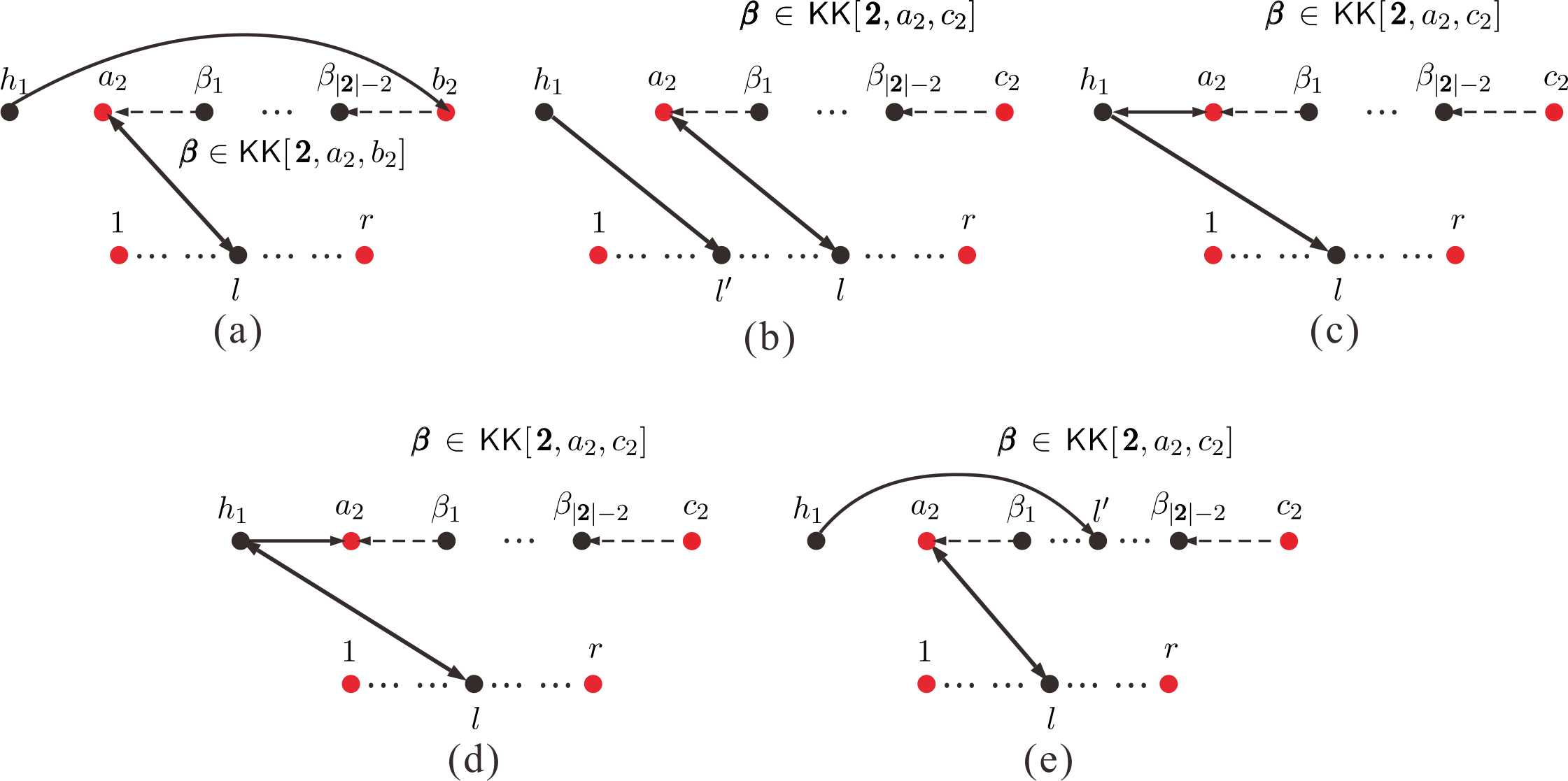
If , the typical graphs are shown by Fig. 4 (a), (b) and (c). Correspondingly, these graphs contribute
| (2.15) | |||||
| (2.16) | |||||
| (2.17) |
where the permutations in and satisfy and respectively. The signs caused by arrows pointing away from the root are absorbed into the coefficients in eqs. (2.15), (2.16) and (2.17), but the signs , induced by the trace are not. Then the sum over all graphs in eq. (2.1) for the amplitude is given by
| (2.18) | |||
where the summation over () and the factor () corresponding to the trace have been absorbed into the notation (), i.e.,
| (2.19) |
The in the second term of eq. (2.18) is arbitrarily fixed because the trace plays as the starting trace in Fig. 4 (b) and (c).

If , the typical graphs are given by Fig. 4 (b), (c), (d) and (e). The expression of Fig. 4 (b) and (c) are already shown by eq. (2.16) and eq. (2.17). The contributions from Fig. 4 (d) and (e) read
| (2.20) | |||||
| (2.21) |
where can be any element in the trace . The sum over all graphs in eq. (2.1) for the amplitude is then written as
| (2.22) | |||
2.3 Induced identities by refined graphs
As pointed in Du:2017gnh, one can induce a nontrivial identity (see eq. (A.11) or eq. (A.12)) of EYM amplitudes by imposing each of the following conditions on the recursive expansion (A.1): (i). the gauge invariance condition of a graviton, (ii). the cyclic symmetry of a gluon trace. When the EYM amplitudes on the LHS of eq. (A.11) and eq. (A.12) are further expanded repeatedly according to eq. (A.1), we finally arrive identities for pure YM amplitudes. Such an identity can also be obtained by imposing the condition (i) or (ii) on eq. (2.1) straightforwardly. As shown in the appendix, we only need to study identities which are induced by conditions of the highest-weight element. Those identities induced by conditions of elements other than the highest-weight one are essentially treated as cases with a smaller set.
If the highest-weight element in the reference order (2.2) is a graviton , the gauge invariance condition of states that the expansion (2.1) vanishes when is replaced by :
| (2.23) |
The corresponding graphs can be obtained by the replacement Fig. 5 (a) 77 7 Although, the arrow in Fig. 5 (a) points away from the root, we do not associate a minus sign with this graph, for an overall sign in the identity eq. (2.23) can always be neglected..
If the highest-weight element in the reference order (2.2) is a gluon trace , the following identity is induced by the replacement
| (2.24) |
for any :
| (2.25) |
This identity is understood as follows: when we consider (for ) (which does not contain the fixed gluon ) as the highest-weight element (see Fig. 5 (b)) and then apply the refined graphic rule, the total contribution of the RHS of eq. (2.1) must vanish. As stated in Du:2017gnh, this identity is essentially a result of the cyclic symmetry of the trace . It is worth pointing out an interesting property Du:2017gnh: when we sum over with the sign , the trace after the replacement Fig. 5 (b) becomes the RHS of Fig. 5 (c) (where is supposed to be ). In the coming sections, we always use the RHS of Fig. 5 (c) to stand for the highest-weight element in the identity (2.25).
3 Identities induced from as combinations of BCJ relations
We now take the identities induced from the amplitude as explicit examples and show that eq. (2.23) and eq. (2.25) can be written as combinations of graph-based BCJ relations (A.15) (thus traditional BCJ relations (A.14)). Critical features of these examples are further summarized.

3.1 Example-1: the identity (2.23) induced from
When the reference order is chosen as , the highest-weight element is the graviton . Thus the expansion (2.1) for the double-trace amplitude induces an identity (2.23) under the replacement . Typical graphs for this identity are given by Fig. 6 (a), (b) and (c) which are correspondingly obtained from Fig. 4 (a), (b) and (c) via the replacement Fig. 5 (a). The total contributions of these graphs are then written as
| (3.1) | |||||
| (3.2) | |||||
| (3.3) |
where , and are already presented in eq. (2.15), eq. (2.16) and eq. (2.17) respectively. Then the full expression of the RHS of the identity (2.23) induced from is given by
| (3.4) |
where a summation notation with a tile is already defined by eq. (2.19).
To investigate the relationship between the induced identity and BCJ relations, we define the standard basis set for a gluon trace by the set of permutations for an arbitrarily fixed end node (i.e. we do not sum over the end node ). Graphically, any two adjacent nodes for a given permutation in the standard basis set are connected by a dashed arrow line pointing towards the node . A starting trace defined by the refined graphic rule is already expressed by the standard basis because an end node of this trace is already fixed. Moreover, all internal traces can be expanded by the standard basis, according to the following nontrivial property:
| (3.5) |
where each graph stands for its full contribution (including coefficients and amplitudes). The LHS of the above equation is an internal trace structure defined by the refined graphic rule. On the RHS, the trace is expressed by the standard basis with one end fixed. The node () on both sides of eq. (3.5) must be connected to a same node outside the trace via the same type of line (i.e., type-2 or type-3 line). The summation notations with a tilde in eq. (3.5) was already defined by eq. (2.19). If a dashed arrow points away from the root, an extra minus should be dressed. We leave the proof of eq. (3.5) in appendix B.

Now we apply the relation (3.5) to the first term of eq. (3.4) for a given . Since the in eq. (3.5) can be chosen arbitrarily, we just choose the (in this example ) as the fixed gluon in the trace of Fig. 6 (b) and (c) for convenience. Then the summation in the first term of eq. (3.4) splits into
| (3.6) |
where and are corresponding to Fig. 7 (a1) and (a2). Substituting eq. (3.6) into eq. (3.4) and introducing the contribution of spurious graph Fig. 7 (a3) by , we rewrite eq. (3.4) as the sum of and which are respectively defined by
| (3.7) |
and
| (3.8) |
In the following, we analyze and in turn and prove that both of them can be expanded in terms of graph-based BCJ relations.

(i). It is easy to see the graphs Fig. 7 (a1), (a3) and Fig. 6 (c) corresponding to the three terms of eq. (3.7) can be reproduced by drawing a type-3 line between a gluon and a node where is the tree structure Fig. 8. Particularly, is given by for Fig. 7 (a1), for Fig. 7 (a3) and for Fig. 6 (c). The kinematic factors of Fig. 7 (a1), (a3) and Fig. 6 (c) can then be uniformly given by . Let us count the sign: Given in eq. (3.7), there is an overall sign which has already been absorbed into the summation notation with a tilde . The sign for each term inside the square brackets is collected as follows: (1). According to the refined graphic rule, any graph with arrows (for both solid and dashed arrow lines) pointing away from the root is associated with a sign . (2). Each of (a1) and (a3) has an extra sign . The above observations further lead to the following pattern:
- •
Once has been chosen, the sign is independent of the choice of because neither nor the extra sign in eq. (3.7) relies on . On another hand, two graphs with adjacent are associated with opposite signs.
- •
All permutations established by the graph with any given have the form
(3.9) Here is introduced as the relative orders between nodes of the tree when the node is considered as the leftmost one. According to the refined graphic rule, when we connect a type-3 line between and , must be nearer to the root than . In other words, for a given permutation in eq. (3.9), can be any node satisfying . Then the total coefficient (which comes from the type-3 line between and ) for the permutation is collected as where (the momentum of the root is always included in this summation).
Altogether, in eq. (3.7) can be reexpressed by
| (3.10) |
where denotes the sign for the graph with (). The for any is fixed as (i). , (ii). if and are two adjacent nodes in . Therefore, the expression in the square brackets is just the LHS of the graph-based BCJ relation (A.15) which has been proven to be a combination of traditional BCJ relations (A.14) (see Hou:2018bwm).
(ii). For , all the permutations established by the graphs Fig. 6 (b), Fig. 7 (a2) and (a3) have the form , where
| (3.11) |
Coefficient for each permutation is collected as . Hence turns to
| (3.12) |
in which satisfy eq. (3.11). Apparently, the expression in the square brackets is just the LHS of a special case of BCJ relation (A.14), which can also be understood as the graph-based BCJ relation (A.15) when the tree graph is the single node .
3.2 Example-2: the identity (2.25) induced from
When the reference order for the expansion (2.1) of the double-trace EYM amplitude is chosen as (i,e., the trace is the highest-weight element), the cyclic symmetry of the trace induces the identity (2.25) where typical graphs are presented as Fig. 4 (b)-(e). According to the discussions in section 2.3, we do the replacement Fig. 5 (b) and then Fig. 5 (c) on the graphs Fig. 4 (b)-(e). Thus graphs Fig. 9 (a)-(d) with the following contributions are obtained correspondingly:
| (3.13) |
in which,
| (3.14) | |||||
Once all graphs are summed over, we arrive the RHS of the induced identity eq. (2.25) for the amplitude :
| (3.15) |
where contributions of all graphs of the form Fig. 9 (a), (b) and (c), (d) were collected as and respectively. Now we prove that both and in eq. (3.15) can be expanded in terms of BCJ relations.

For the part in eq. (3.15), the summation over is nothing but just the summation over all nodes where is the tree graph Fig. 10 (a). All permutations established by the graphs Fig. 9 (a), (b) with a given and a given have the form
| (3.16) |
Here, and denotes the relative orders of nodes in when is considered as the leftmost one. Based on a similar discussion with the example-1 in section 3.1, we find the following patterns: (1). The coefficients ( for Fig. 9 (a) and for Fig. 9 (b)) corresponding to a same with different choices of are collected as ; (2). Any two graphs, where are chosen as adjacent nodes, have opposite signs. Then the part in eq. (3.15) is expressed by
| (3.17) | |||||
Here is the sign for a graph with . Since has been extracted as an overall sign, we have . If are two adjacent nodes, we have . Obviously, the expression in the square brackets is nothing but (up to a total minus) the LHS of a graph-based BCJ relation (A.15). As a result, is a combination of traditional BCJ relations.
The part in eq. (3.15) can be analyzed following a parallel discussion with but replacing the tree graph by (see Fig. 10 (b)) for and replacing by :
| (3.18) |
where and . Again, the ’s for adjacent choices of have the opposite signs. Up to a total sign, the expression in the square brackets is just the LHS of graph-based BCJ relation (A.15), where the tree graph for a given is Fig. 10 (b). Thus, we conclude that is a combination of BCJ relations.
3.3 Common features of the examples
Now let us extract some common features from the examples, which will be extended to general cases in the next section.

(i). Expressing traces by standard basis In example-1, the trace played as an internal trace in Fig. 6 (a) and a starting trace in either Fig. 6 (b) or (c). In the latter cases, the trace was already expressed by the standard basis, i.e., one end of the trace, the gluon , was fixed. In the former case, both ends of the trace were not fixed (in other words both are summed over). In order to expand the trace in Fig. 6 (a) by the standard basis, we have made used of the splitting trace relation (3.5), in which the fixed node was conveniently chosen as the same element (i.e. ) with that in Fig. 6 (b) and (c).
(ii). Skeletons and components We define skeletons by removing all type-3 lines from the graphs where all traces, except the highest-weight element in (if it is a trace), are already expressed by the standard basis. Since each graph defined by the refined graphic rule is a connected tree graph, its skeleton must be a disconnected graph. Each maximally connected subgraph of a skeleton is called a component. A typical skeleton in example-1 is given by Fig. 11 (a) (for , ) which consists of three components. Skeletons in example-2 have two distinct structures, Fig. 11 (b) and (c), each of which has two components. From the examples, we can see any skeleton must have at least two components that involve the highest-weight element (graviton or trace) and the trace respectively.

(iii). The final upper and lower blocks Any graph in the examples can be reproduced by connecting a type-3 line between the final upper and lower blocks which are two mutually disjoint connected subgraphs and respectively contain the highest-weight element and the trace . In example-2, each of the skeletons Fig. 11 (b) and (c) already consists of only two disjoint connected subgraphs and which serve as the final upper and lower blocks. In example-1, there are three components in the skeleton Fig. 11 (a). A typical configuration of the final upper and lower blocks is constructed when we connect in Fig. 11 (a) to either (i). (see Fig. 12 (a)) or (ii). an element in via a type-3 line (see Fig. 12 (b)).
(iv). Physical and spurious graphs For a given configuration of the final upper and lower blocks and , we can connect two nodes and (recalling that the gluon is always excluded) via a type-3 line. Then a fully connected graph is constructed. In example-2, the graphs Fig. 9 (a), (b) (and Fig. 9 (c), (d)) are reproduced by connecting the final upper and lower blocks in Fig. 11 (b) (and Fig. 11 (c)) via a type-3 line. Similarly, the graphs Fig. 7 (a1), Fig. 6 (c) (and Fig. 7 (a2), Fig. 6 (b)) in example-1 are constructed from Fig. 12 (a) (and (b)). All the graphs Fig. 6 (b), (c), Fig. 7 (a1), (a2) and Fig. 9 (a)-(d) are graphs in standard basis which are directly defined by the refined graphic rule. These graphs are called physical graphs. The spurious graph Fig. 7 (a3), which is not defined by the refined graphic rule, can be reproduced from either Fig. 12 (a) (connecting with ) or Fig. 12 (b) (connecting with ). In the former case, a minus sign is introduced so that the spurious graph constructed by distinct ways cancel with one another. Therefore, for any skeleton, the sum of all physical graphs can be given by (1). summing over all possible configurations of the final upper and lower blocks , , (2). for a given and , connecting two nodes and via a type-3 line and summing over all possible choices of , (in other words summing over all possible physical and spurious graphs corresponding to and ).
(v). Induced identities as combinations of graph-based BCJ relations A crucial observation is that the sum over all the graphs corresponding to a given configuration of the final upper and lower blocks and (i.e. either or in each example) is a combination of graph-based BCJ relations (A.15).
4 General study
To investigate the general induced identities (2.23) and (2.25) in a unified way, we write them as
| (4.1) |
where the graphs are obtained by imposing the replacement Fig. 5 (a) or (b), which corresponds to eq. (2.23) or eq. (2.25), on the graphs in eq. (2.1).
When we introduce skeletons by deleting all type-3 lines from the graphs and expressing all traces by standard basis according to eq. (3.5), eq. (4.1) is rearranged as
| (4.2) |
In the above equation, the summation notation means that all possible skeletons are summed over and the signs and/or accompanying to the traces in each are absorbed. The factor denotes the kinematic factor corresponding to the skeleton . Since a skeleton does not involve any type-3 line, only consists of and factors. In the expression inside the square brackets, all possible physical graphs (i.e. graphs generated by refined graphic rule with all internal traces expressed by the standard basis) containing the skeleton and all permutations for each graph are summed over. The factor in eq. (4.2) stands for the product of all factors that are presented by the type-3 lines in . Those signs caused by arrows pointing away from the root and the extra signs caused by the second term of eq. (3.5) are all collected as .

As observed in section 3.3, all physical graphs involving a given skeleton can be generated by connecting the components via type-3 lines in a proper way: (i). first generate all possible configurations of the final upper and lower blocks ; (ii). then connect a type-3 line between two nodes and appropriately. One should take care of the step (ii) because spurious graphs may also be produced. Nevertheless, the spurious graphs in fact all cancel out in the examples. Hence we suppose that the expression in the square brackets in eq. (4.2) can be generally written as
| (4.3) |
Here, is the product of all factors corresponding to the given configuration of the final upper and lower blocks , , while is the factor corresponding to the type-3 line between and . The first summation in eq. (4.3) is taken over all possible configurations of the final upper and lower blocks , for the skeleton . In the square brackets, all choices of nodes and as well as the permutations defined by the (physical or spurious) graph (determined by , , and ) are summed over. The sign for the (physical or spurious) graph is denoted by .
In this section, we study eq. (4.3) schematically. We first classify components of skeletons, then show how to construct the final upper and lower blocks from a given skeleton . After that, we show all spurious graphs cancel out. Thus the summation over all possible choices of and is equivalent to summing over all possible physical graphs for given and . At last, we demonstrate that the expression inside the square brackets in eq. (4.3) is a combination of BCJ relations.


4.1 Skeletons and components
When all type-3 lines (i.e. factors) are removed, a graph becomes a skeleton . To analyze possible structures of components which are maximally connected subgraphs of , we should look into the inner structure of a chain via expanding eq. (2.6) by eq. (• ‣ 2.1), eq. (• ‣ 2.1) and eq. (3.5). According to whether the starting node is the highest-weight element in the reference order (defined in eq. (2.2)) or not, we carry out the discussion as follows:
- •
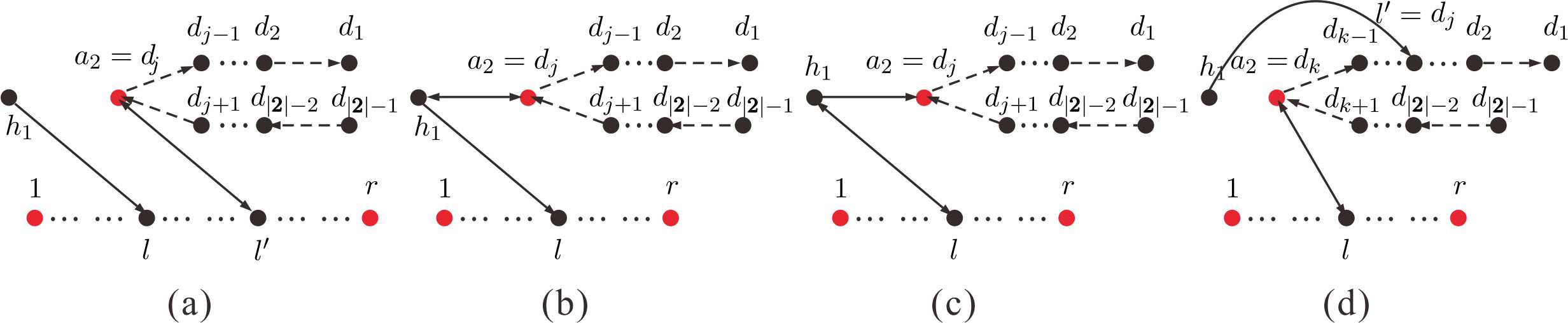
(i). If the starting node of a chain is not the highest-weight element , a graph corresponding to this chain can only have the general pattern Fig. 13 (a). Now we comment on crucial features of Fig. 13 (a): (1). Distinct sectors are separated by type-3 lines. The sector containing the starting (ending) node is called the starting (ending) sector. Other sectors between the starting and ending sectors are mentioned as internal sectors. (2). The possible structures inside the boxes in Fig. 13 (a) are given by Fig. 13 (d) (where two gravitons are connected by a type-1 line) and Fig. 13 (e), (f) (which involve a gluon trace expressed by standard basis). (3). If a chain Fig. 13 (a) contains only one sector, the sector must be the ending sector. (4). If the starting element of a chain is a gluon trace, there must be no graviton on the left hand side of the box in the starting sector, as shown by Fig. 13 (f). (5). Other structures of a chain are forbidden because the substructures in Fig. 13 (c) are not allowed by (eq. (2.6)) (in other words, for a graviton involves neither nor ).
- •
(ii). If the starting node of a chain is the highest-weight element , its corresponding graph must have the general pattern Fig. 13 (b), where the highest-weight element (graviton or trace) is already replaced according to Fig. 5 (a) (for a graviton) or Fig. 5 (b) and (c) (for a gluon trace). An important feature is the chain Fig. 13 (b) has at least two sectors, which follows from the fact that structures in Fig. 13 (c) are forbidden.
Having the above discussions, sectors of chains can be easily classified as Fig. 14. In a full graph , nodes of any sector may play as the ending nodes of other chains. When all type-3 lines are removed, each sector in a skeleton thus can be attached by the type-3 sectors Fig. 14 (c) (or equivalently ending sectors) of other chains. Consequently, components in a skeleton can be classified by the following way.
- •
Type-I component: A component consisting of a type-I sector Fig. 14 (a) and possible type-III sectors Fig. 14 (c) whose arrow lines point towards the type-I sector Type-I components can further be classified according to different structures inside the box of Fig. 14 (a): If the box contains the structure Fig. 13 (d), as shown by Fig. 15 (a), this component is called a type-IA component. Else, if the structure in the box is given by Fig. 13 (e) or (f), as shown by Fig. 15 (b), the component is called a type-IB component. We define the kernel of a type-I component by (i). the type-1 line of a type-IA component (see Fig. 15 (a)), (ii). the type-4 line that is attached to the unfixed end node of the trace (in standard basis) inside a type-IB component (see Fig. 15 (b)). For a given reference order, any type-IA and -IB component is divided into two parts by the kernel: the part involving the highest-weight node (although a trace is considered as a single object in the reference order, the fixed node is always considered as the highest-weight node of this trace and it carries the weight of the full trace in the reference order) of this component is called the top side, while the opposite part is called the bottom side.
- •
Type-II component: A component consisting of a type-II sector Fig. 14 (a) and possible type-III sectors whose arrows point towards the type-II sector If the structure in the box of the type-II sector is Fig. 13 (g) (i.e. the highest-weight element is a graviton), this component is called a type-IIA component (see Fig. 16 (a)). If the structure in the box is a gluon trace Fig. 13 (h), the component is called a type-IIB component (see Fig. 16 (b)).
- •
Type-III component: A component consisting of the trace and possible type-III sectors with arrows pointing towards the trace (see Fig. 16 (c))
Since the chain Fig. 13 (b) that is lead by the highest weight node has at least two sectors, a skeleton must at least contain two components: the type-II and the type-III components. In general, Type-I components may also be involved in a skeleton. All those graphs corresponding to a given skeleton are reproduced by connecting type-3 lines between components of a skeleton in an appropriate way.
Multi-trace from single-trace
It is worth pointing out that the refined graphic rule given in section 2 can be obtained from the rule for identities induced from single-trace amplitudes (which was presented in Hou:2018bwm) by an appropriate replacement. Particularly, we consider a single-trace amplitude where we have gravitons . When we replace gravitons, e.g., by gluon traces , we get the multi-trace amplitude with . Such replacement is reflected in the refined graphic rule via replacing the reference order and chains with only gravitons by those with gravitons and/or gluon traces. The corresponding replacement for coefficients are given by
| (4.4) |
where , are the half polarizations and strength tensors of gravitons, while and are generalized polarizations and generalized strength tensors for gravitons and/or gluon traces (see eq. (• ‣ 2.1) and eq. (• ‣ 2.1)). Graphically, this replacement is given by
| Fig. 1 (a) | |||||
| Fig. 1 (b) | (4.5) |
For identities induced from a single-trace amplitude, the highest-weight element (graviton) is further given by (see Fig. 5 (a)). In the corresponding multi-trace case, the highest-weight element can either be a graviton (if it is not replaced by a trace) or be replaced by a gluon trace. The latter is described via replacing the node (the highest-weight graviton for identity induced from single-trace amplitude) by the RHS of Fig. 5 (c).
Now we look into the inner structure of a chain by further expanding internal gravitons on the LHS of eq. (4.4) according to . On the RHS, internal gravitons are also expanded by , while internal gluon traces are expanded according to the relation eq. (3.5). Although this expansion of gluon trace does not affect the tensor for a given and (see eq. (• ‣ 2.1)), it splits the graphs corresponding to the trace into the standard basis. Hence, the replacement (for an internal graviton ) is achieved graphically through replacing the first (second) graph in Fig. 1 (b) by the first (second) graph on the RHS of eq. (3.5) (for a given ). It follows that the general chain structures Fig. 13 (a) and (b) are obtained from those chain structures for the single-trace case Hou:2018bwm (where only type-IA, type-IIA and type-III sectors are allowed) by incorporating more types of sectors: type-IB and type-IIB sectors which reflect structures of gluon traces. Consequently, the full classification of components in multi-trace cases can be given by enlarging the families of the type-I and the type-II components that were defined in Hou:2018bwm:
| Type-I components | |||||
| Type-II components | (4.6) |
where the type-IIA and type-IIB components are respectively the highest-weight components of the identities (2.23) and (2.25). All the above discussions allow us to borrow some crucial conclusions from the single-trace case Hou:2018bwm:
- •
(i) When keeping track of chains in the single-trace case Hou:2018bwm, one can build all possible physical graphs corresponding to a skeleton by connecting type-3 lines between components properly (see appendix D in Hou:2018bwm). This construction can be immediately generalized to multi-trace cases by the enlargement (4.6).
- •
(ii) As proved in Hou:2018bwm (see sections 6.1, 6.2 and appendix D of Hou:2018bwm), all the physical graphs in the single-trace case, which are corresponding to a given skeleton and are constructed by the above step, can be reproduced by (1). constructing the final upper and lower blocks, (2). connecting the final upper and lower blocks via a type-3 line appropriately. In multi-trace cases, we just follow the same construction rule but enlarging the type-I and type-II classes of components according to (4.6).
- •
(iii) As pointed in section 6.3 of Hou:2018bwm, in the single-trace case, the sum over all physical graphs which are produced by (ii) can be further written as the sum of all physical and spurious graphs (those graphs which are not directly constructed from the refined graphic rule). The latter all cancel out after summation. Again, the spurious graphs for single-trace induced identities can be straightforwardly extended to multi-trace cases by the help of (4.6) and they all cancel out (we have seen this cancellation by the examples in section 3).
In the coming two subsections, we display the construction rule of the final upper and lower blocks as well as the construction of physical and spurious graphs without a proof. In fact, all the proofs follow from discussions parallel with those in the single-trace case Hou:2018bwm.
4.2 The final upper and lower blocks
Now we provide the general rule for constructing all possible configurations of the final upper and lower blocks corresponding to a given skeleton :
- •
Step-1 For any skeleton , we define the reference order of all type-I components (including type-IA and type-IB components) by the relative order of the highest-weight nodes therein. In other words, the weight (i.e. the position in ) of a component inherits from its highest-weight node. For example, suppose there are three type-I components (IA and/or IB) , , and with the corresponding highest-weight nodes (graviton or a gluon) , and . If the weights have the relation , the reference order of these components is then given by the ordered set . We further define the upper block and lower block as the components respectively containing the highest-weight element (graviton or trace) and the trace . At the beginning, the upper and the lower blocks are nothing but the type-II and the type-III components.
- •
Step-2 Supposing the reference order of components is , pick out the highest-weight component as well as arbitrary components , , …, (the relative order of these components is not necessary the same relative order in ). Construct a chain of components towards either the upper block or the lower block as follows
Here the subscripts and respectively denote the top and bottom sides of a type-I component, which are separated by a comma88 8 Notations here are slightly different from those in Hou:2018bwm.. The double arrow line ‘’ between two components stands for the type-3 line (i.e. ), which connects any two nodes belonging to the corresponding regions. For example, if the chain of components has the form , the two ends and of the type-3 line between the components and must belong to and respectively. After this step, we redefine the reference order of components as well as the upper and lower blocks by:
(4.8) - •
Step-3 Repeating step-2 with the new defined , and iteratively until the ordered set becomes empty, we get a graph with only two mutually disjoint subgraphs: the final upper and lower blocks and .

4.3 Physical and spurious graphs
For a given configuration of the final upper and lower blocks and which are constructed previously, a fully connected graph in eq. (4.3) is produced by connecting arbitrary two nodes and via a type-3 line. As pointed in section 3, such a graph can be either a physical graph or a spurious one. We have already stated that physical and spurious graphs can be obtained from those in single-trace case Hou:2018bwm by the enlargement (4.6). As a result, a spurious graph has the structure Fig. 17, where the chain starting form the highest-weight element (graviton for the identity (2.23) and gluon for the identity (2.25)) and ending at the root passes through single sides of some type-IA and/or type-IB components which respectively belong to the chains of components .
In order to display more details of spurious graphs, we define the weight of a chain by the weight of the starting component (equivalently the highest-weight component) of . As pointed in Hou:2018bwm, if the lowest-weight chain among in Fig. 17 is , we must have and . Following a discussion which is parallel with that in Hou:2018bwm, we conclude that all the chains (and structures attached to them) belong to the final lower block , while (and structures attached to them) belong to the final upper block . Only the lowest-weight chain (among ) can live in either or . Correspondingly, the type-3 line (colored by red in Fig. 17) on either the LHS or the RHS of is considered as the one between the final upper and lower blocks. Thus a given spurious graph is corresponding to two distinct configurations of and . In other words, all spurious graphs must appear in pairs! This fact allows us to associate a pair of spurious graphs with opposite signs so that all spurious graphs cancel out.
By the help of the above discussion, we now determine the sign in eq. (4.3) for a (physical or spurious) graph :
- •
(i). As proposed in Hou:2018bwm, a graph is accompanied by a sign , where is the number of spurious components living in the final upper block for a given in eq. (4.3). For the typical spurious graph Fig. 17, , if belongs to the final upper block , while , if belongs to the final lower block . Hence spurious graphs cancel in pairs precisely.
- •
(ii). Another sign which should be taken into account is introduced by the relation eq. (3.5). Particularly, if the arrow of the kernel in a type-IB component (see Fig. 15 (b)) is pointing away from the root (i.e. the second term of eq. (3.5)), this component should be dressed by an extra minus. Since the choice of in eq. (4.3) does not affect the direction of arrows in the final lower block , the number of such type-IB components only depends on , and the choice of in eq. (4.3). We use to denote this number, the resulting sign is then written as .
- •
(iii). For any graph, the total number of arrows pointing away from the root induces the third sign (as required by the refined graphic rule), where and count the corresponding numbers in (for ) and . The extra minus is caused by the type-3 line between and .
To sum up, the sign for any (physical or spurious) graph is given by
| (4.9) |
For a physical graph , there is no spurious component, thus . For identities induced from single-trace amplitudes, vanishes and the sign (4.9) turns into the one given in Hou:2018bwm.
4.4 Expanding induced identities in terms of BCJ relations

We are now ready to show the expression in the square brackets in eq. (4.3), i.e.
| (4.10) |
for a given configuration of the final upper and lower blocks , is the LHS of the graph-based BCJ relation (A.15) (hence a combination of traditional BCJ relations (A.14)). Here a graph in the above expression is a physical or a spurious graph which is constructed by connecting two nodes , via a type-3 line. Our discussion is carried out by the follow steps:
- •
(i). According to the refined graphic rule, permutations in eq. (4.10) are independent of the line styles in . Therefore, all lines in can be replaced by dashed lines (with no arrow) which only characterize the relative positions of nodes in , as shown by Fig. 18. Apparently, for a given configuration of the final upper and lower blocks , and a given choice of , the corresponding permutations satisfy
(4.11) where and denote the permutations established by and when and the root are the leftmost elements respectively. Since and are fixed as the first and the last elements in eq. (4.10), they should be excluded from . The means situates before in the permutation, i.e. . Noting that the choice of is independent of the relative orders and , we rewrite the summations in eq. (4.10) as follows
(4.12) - •
(ii). For a given permutation , one can collect together the coefficients in eq. (4.11) with different choices of . Specifically, only those satisfying in have nonzero contributions and the sign (4.9) is totally independent of . Hence, all the factors for a given are collected as where (the gluon is always included as the leftmost in this summation). Meanwhile, the last two summations in eq. (4.12) turns into
(4.13) - •
(iii). As illustrated by appendix C, the sign in eq. (4.10) has the following pattern. Two graphs with and where are adjacent to each other must be associated with opposite signs. Hence one can extract the sign eq. (4.9) for a graph with as an overall factor and then the sign for an arbitrary choice of node is given by
(4.14) where is defined by (i). , (ii). for two adjacent nodes and ().
When all the above are taken into account, eq. (4.10) is finally expressed by
| (4.15) |
where the summation over was extracted out because it is independent of the choice of . The expression in the square brackets in eq. (4.15) is nothing but the LHS of the graph-based BCJ relation (A.15).
5 Conclusions
In this paper, we provided the refined graphic rule for expanding tree level multi-trace EYM amplitudes in terms of color-ordered YM amplitudes. When the gauge invariance condition of a graviton and the cyclic symmetry of a gluon trace were imposed, this expansion induced two identities (2.23) and (2.25) respectively. By extending the analysis for the single-trace case Hou:2018bwm to an arbitrary multi-trace induced identity, we demonstrated that eq. (2.23) and eq. (2.25) can finally be expressed as a combination of graph-based BCJ relations (thus traditional BCJ relations).
There are several related topics that deserve further study: (i). First, how to understand the induced identities from the view of string theory? String theory studies of the expansions of EYM amplitudes have been established in Stieberger:2016lng; Schlotterer:2016cxa; He:2018pol; He:2019drm, while BCJ relations have also been proven in string theory BjerrumBohr:2009rd; Stieberger:2009hq. Hence it is reasonable to expect a string-theory approach to both induced identities and graph-based BCJ relations. (ii). Second, it is worth investigating the induced identities in various theories systematically. In Zhou:2019mbe, a unified web of expansions of amplitudes was founded with the help of the unifying relation Cheung:2017ems, which inspires that the induced identities may exist in many other theories. (iii). Third, the YM expansion of EYM amplitudes, which have been used in this paper, is in KK basis Kleiss:1988ne. As pointed in Feng:2019tvb, this expansion can be extended to BCJ basis Bern:2008qj. We expect that the refined graphic rule can also be generalized to expansions in BCJ basis Bern:2008qj. (iv). Last but not least, a kinematic algebra for constructing BCJ numerators in the MHV sector was proposed Chen:2019ywi. It seems that distinct sectors of numerators are corresponding to graphs with different numbers of type-IA kernels. Thus, one may provide a general rule for constructing all sectors of BCJ numerators, with the help of refined graphic rule.
Acknowledgments
The authors are grateful to Chih-Hao Fu, Song He, Xiaodi Li, Hui Luo, Gang Yang, Yihong Wang and Yong Zhang for helpful discussions or/and valuable comments. This work is supported by NSFC under Grant Nos. 11875206, 11847309, Jiangsu Ministry of Science and Technology under contract BK20170410 as well as the “Fundamental Research Funds for the Central Universities”.
Appendix A Recursive expansions and BCJ relations
In this section, we review the recursive expansions of multi-trace EYM amplitudes and the BCJ relations for YM amplitudes.
A.1 Recursive expansions of multi-trace EYM amplitudes
When all gravitons and gluon traces are collected into the set , a tree level multi-trace EYM amplitude where can be briefly expressed by . As proven in Du:2017gnh, this multi-trace amplitude satisfies the following recursive expansion relation:
| (A.1) |
In the expansion (A.1), we have picked out an arbitrary element (a graviton or a gluon trace) from , which is called the fiducial element. Apparently, can be either a graviton or a gluon trace. On the RHS of eq. (A.1):
- •
The first summation is taken over (i). all possible splittings of the set into two subsets , and (ii). all permutations of elements in for a given splitting.
- •
For a given splitting of and a given permutation of elements in , the summation is defined as follows
if is a graviton: (A.2) if is a gluon trace: (A.3) This means we sum over all possible choices of the ordered pair of gluons for all traces . If the fiducial element is also a trace, namely , we should fix an arbitrary gluon and then sum over all choices of in this trace. For a given choice of and , a gluon trace (including if it is also a trace) can always be written into the form where and are the two ordered sets of gluons separated by and . The sign in eq. (A.2) and eq. (A.3) for each trace is defined as where is the number of elements in . Permutations (for a given ) and (for a given ) in eq. (A.2) and/or eq. (A.3) which satisfy
(A.4) (A.5) are also summed over.
- •
Supposing that the permutation of elements in in the first summation (see eq. (A.1)) is given by , ,…, and the gluon pairs in the second summation are ( can be if the fiducial element is a gluon trace ), we sum over all permutations satisfying
(A.6) Here the traces in the ordered set are no longer considered as single elements but considered as proper permutations of all gluons in them. Particularly, if denotes a gluon trace and this trace can be written as for a given choice of ordered pair , we should replace in eq. (A.6) by a permutation where satisfies eq. (A.4). Similarly, if the fiducial element is also a trace, say , it must be replaced by a permutation where satisfies eq. (A.5). Then the summation over in eq. (A.1) means summing over all possible shuffle permutations in eq. (A.6).
- •
A.2 Identities induced from multi-trace EYM amplitudes
Symmetries of multi-trace EYM amplitudes, together with the recursive expansion (A.1), induce nontrivial identities for EYM amplitudes with fewer gravitons and/or gluon traces Du:2017gnh. There are two symmetries under consideration in this paper: the gauge invariance condition for a graviton and the cyclic symmetry of a gluon trace.
Muti-trace EYM amplitude satisfies gauge invariance condition, which states that the amplitude has to vanish once half polarization of a graviton is replaced by the momentum . If this replacement is performed on the RHS of the recursive expansion (A.1), we should consider two distinct situations:
- •
If the fiducial element is a graviton (i.e. eq. (A.1) is type-I expansion), the gauge invariance condition for induces a nontrivial relation between EYM amplitudes with fewer gravitons
(A.11) - •
If is not the fiducial one, it may belong to either or in eq. (A.1) . Terms with have to vanish due to the antisymmetry of the strength tensor , while terms with have to vanish due to gauge invariance of amplitudes with fewer gravitons.
Therefore, the only nontrivial identity induced by the gauge invariance condition of a graviton is eq. (A.11) which is called type-I identity in Du:2017gnh.
Another identity (called type-II identity in Du:2017gnh) is induced from the expansion (A.1) where the fiducial element is a gluon trace . In particular, we notice that the end element can be chosen arbitrarily in the fiducial trace . This arbitrariness is essentially caused by the cyclic symmetry of the trace Du:2017gnh and indicates the following identity
| (A.12) |
where is defined by
| (A.13) |
Here we removed from the trace first, then shuffled these permutations according to eq. (A.6). The , , …, is a permutation of elements in .
A.3 BCJ relations
Tree level color-ordered YM amplitudes satisfy the following traditional BCJ relation BjerrumBohr:2009rd; Chen:2011jxa:
| (A.14) |
where and are two ordered sets of external gluons, denotes the sum of all momenta of gluons satisfying .
In Hou:2018bwm, the following graph-based BCJ relation for YM amplitudes was proposed
| (A.15) |
Here, is an arbitrary permutation of elements in and is an arbitrary connected tree graph. When a node is chosen as the leftmost element, the tree graph establishes permutations as follows (i). For two adjacent nodes and , if is nearer to than , we have , (ii). If there are subtree structures attached to a same node, we should shuffle the permutations established by these subtrees together. The factor is a relative sign depending on the node . This factor is determined by the following steps. (i). Choose an arbitrary node and require . (ii). For arbitrary two adjacent nodes and , we have . As already proven in Hou:2018bwm, the graph-based BCJ relation (A.15) can always be written as a combination of the traditional ones (A.14).
Appendix B Proof of eq. (3.5)
To prove eq. (3.5), we focus on a term with a given choice of in eq. (3.5) and prove the following stronger relation:
| (B.1) |
where the denotes a tree structure which is attached to the node . In fact, all these nodes in the trace can be attached by arbitrary tree structures and the relation (B.1) still holds. Once all are summed over, we arrive the relation (3.5).
Suppose the gluons in trace are in the cyclic order . Without loss of generality, and are respectively chosen as , . Then the permutations on the LHS of eq. (B.1) are explicitly displayed by
| (B.2) | |||||
with a sign (the overall sign coming from has been neglected). Here denotes the nearest to node in and are the permutations established by the tree . The notation means the position of in the permutation is less than that of . The second line of eq. (B.2), where we shuffled with the full trace and required the node is always on the left of the node , is apparently equivalent to the first line.
On the RHS of eq. (B.1), we assume that the is chosen as (). The case with follows from a similar discussion. Then permutations in the first term on the RHS of eq. (B.1) is given by
| (B.3) |
with the sign . The permutations in the second term of the RHS of eq. (3.5) are given by the following two steps:
- •
First shuffle the gluons in the trace so that and become the two ends of the trace. Then the permutations are explicitly given by
(B.4) which is associated with a sign . These permutations can be classified according to the relative orders between the and elements in the set :
(B.5) - •
According to the relative orders between and , permutations in eq. (B.6) splits into and . It is easy to see
| (B.7) |
Hence the contributions from and for all must cancel one another. The remaining nonzero terms are the two boundaries
| (B.8) | |||||
with the signs and respectively. An extra minus which is introduced from the second term of eq. (B.1) must also be taken into account. Hence the permutations are same with the permutations in eq. (B.3), with an opposite sign. As a result, they cancel with each other. The remaining permutations are nothing but the permutations (B.2) with the corrected sign. Therefore, we have proven the relation (B.1) for a given . After summing over all possible choices of the pairs, the proof of eq. (3.5) is completed.

Comments on the proof: In the above proof, the tree structure is always treated separately from the trace in each step (i.e. it is shuffled with the full trace with a proper constraint, as shown in eqs. (B.2), (B.3), (B.6), (B.8)). Thus manipulations on nodes inside the trace are independent of . This observation allows us to generalize eq. (3.5) to cases where more tree structures are attached to nodes in the trace straightforwardly.
Appendix C The sign in eq. (4.10)
In eq. (4.10), the graph is constructed by connecting and via a type-3 line. As mentioned before, the sign for such a graph is dependent of the choice of but independent of the choice of . Now we show that two graphs with choosing adjacent must have opposite signs. To see this, we study all possible structures presented by Fig. 19 (a)-(e), where is adjacent to (), as follows.
(i). As shown by Fig. 19 (a), nodes and connected by a type-3 line must belong to a same (top or bottom) side of a type-IA or type-IB component. In this case, each one of , and is the same for choosing two adjacent ’s. But the numbers in eq. (4.9) for and differ by one because the type-2 line between and has opposite directions for these two cases.
(ii). If and are connected by a type-4 line, they must belong to a same type-IB component. If the type-4 line is not the kernel of the type-IB component, the structure is given by Fig. 19 (b). In this case, and must belong to a same side of the component. The numbers for choosing and should differ by one because the type-4 line between and has opposite directions. Each of , and in eq. (4.9) is the same for both choices of .
(iii). If the two adjacent nodes and connected by a type-4 line belong to opposite sides of a type-IB component, the type-4 line must be the kernel of the type-IB component (as shown by Fig. 19 (c)). In this case, each of , and for and differ by one but is the same.
(iv). If and are connected by a type-1 line which must be the kernel of a type-IA component (as shown by Fig. 19 (d)), only the number for choosing and differ by one. Any of , and is the same for the two choices of .
(v). If and are connected by a type-3 line as shown by Fig. 19 (e), only for choosing and differ by one. Any other number is the same for the two choices.
Therefore, in all the above cases, for choosing and , where are two adjacent nodes, must differ by an odd number. In other words, two graphs with adjacent ’s have opposite signs.
References
- (1) L. Hou and Y.-J. Du, A graphic approach to gauge invariance induced identity, JHEP 05 (2019) 012, [arXiv:1811.12653].
- (2) Y.-J. Du, B. Feng, and F. Teng, Expansion of All Multitrace Tree Level EYM Amplitudes, JHEP 12 (2017) 038, [arXiv:1708.04514].
- (3) C.-H. Fu, Y.-J. Du, R. Huang, and B. Feng, Expansion of Einstein-Yang-Mills Amplitude, JHEP 09 (2017) 021, [arXiv:1702.08158].
- (4) M. Chiodaroli, M. Gunaydin, H. Johansson, and R. Roiban, Explicit Formulae for Yang-Mills-Einstein Amplitudes from the Double Copy, JHEP 07 (2017) 002, [arXiv:1703.00421].
- (5) F. Teng and B. Feng, Expanding Einstein-Yang-Mills by Yang-Mills in CHY frame, JHEP 05 (2017) 075, [arXiv:1703.01269].
- (6) S. Stieberger and T. R. Taylor, New relations for Einstein-Yang-Mills amplitudes, Nucl. Phys. B913 (2016) 151–162, [arXiv:1606.09616].
- (7) D. Nandan, J. Plefka, O. Schlotterer, and C. Wen, Einstein-Yang-Mills from pure Yang-Mills amplitudes, JHEP 10 (2016) 070, [arXiv:1607.05701].
- (8) L. de la Cruz, A. Kniss, and S. Weinzierl, Relations for Einstein-Yang-Mills amplitudes from the CHY representation, Phys. Lett. B767 (2017) 86–90, [arXiv:1607.06036].
- (9) O. Schlotterer, Amplitude relations in heterotic string theory and Einstein-Yang-Mills, JHEP 11 (2016) 074, [arXiv:1608.00130].
- (10) R. Britto, F. Cachazo, and B. Feng, New recursion relations for tree amplitudes of gluons, Nucl. Phys. B715 (2005) 499–522, [hep-th/0412308].
- (11) R. Britto, F. Cachazo, B. Feng, and E. Witten, Direct proof of tree-level recursion relation in Yang-Mills theory, Phys. Rev. Lett. 94 (2005) 181602, [hep-th/0501052].
- (12) Y.-J. Du and Y. Zhang, Gauge invariance induced relations and the equivalence between distinct approaches to NLSM amplitudes, JHEP 07 (2018) 177, [arXiv:1803.01701].
- (13) Y.-J. Du and C.-H. Fu, Explicit BCJ numerators of nonlinear sigma model, JHEP 09 (2016) 174, [arXiv:1606.05846].
- (14) J. J. M. Carrasco, C. R. Mafra, and O. Schlotterer, Abelian Z-theory: NLSM amplitudes and ’-corrections from the open string, JHEP 06 (2017) 093, [arXiv:1608.02569].
- (15) Y.-J. Du and F. Teng, BCJ numerators from reduced Pfaffian, JHEP 04 (2017) 033, [arXiv:1703.05717].
- (16) R. Kleiss and H. Kuijf, Multi - Gluon Cross-sections and Five Jet Production at Hadron Colliders, Nucl. Phys. B312 (1989) 616–644.
- (17) Z. Bern, J. J. M. Carrasco, and H. Johansson, New Relations for Gauge-Theory Amplitudes, Phys. Rev. D78 (2008) 085011, [arXiv:0805.3993].
- (18) N. Arkani-Hamed, L. Rodina, and J. Trnka, Locality and Unitarity from Singularities and Gauge Invariance, arXiv:1612.02797.
- (19) F. Cachazo, S. He, and E. Y. Yuan, Scattering equations and Kawai-Lewellen-Tye orthogonality, Phys. Rev. D90 (2014), no. 6 065001, [arXiv:1306.6575].
- (20) F. Cachazo, S. He, and E. Y. Yuan, Scattering of Massless Particles in Arbitrary Dimensions, Phys. Rev. Lett. 113 (2014), no. 17 171601, [arXiv:1307.2199].
- (21) F. Cachazo, S. He, and E. Y. Yuan, Scattering of Massless Particles: Scalars, Gluons and Gravitons, JHEP 07 (2014) 033, [arXiv:1309.0885].
- (22) F. Cachazo, S. He, and E. Y. Yuan, Scattering Equations and Matrices: From Einstein To Yang-Mills, DBI and NLSM, JHEP 07 (2015) 149, [arXiv:1412.3479].
- (23) C. S. Lam and Y.-P. Yao, Role of Mb̈ius constants and scattering functions in Cachazo-He-Yuan scalar amplitudes, Phys. Rev. D93 (2016), no. 10 105004, [arXiv:1512.05387].
- (24) C. S. Lam and Y.-P. Yao, Evaluation of the Cachazo-He-Yuan gauge amplitude, Phys. Rev. D93 (2016), no. 10 105008, [arXiv:1602.06419].
- (25) N. E. J. Bjerrum-Bohr, J. L. Bourjaily, P. H. Damgaard, and B. Feng, Analytic Representations of Yang-Mills Amplitudes, arXiv:1605.06501.
- (26) R. Huang, Y.-J. Du, and B. Feng, Understanding the Cancelation of Double Poles in the Pfaffian of CHY-formulism, arXiv:1702.05840.
- (27) X. Gao, S. He, and Y. Zhang, Labelled tree graphs, Feynman diagrams and disk integrals, JHEP 11 (2017) 144, [arXiv:1708.08701].
- (28) S. He, G. Yan, C. Zhang, and Y. Zhang, Scattering Forms, Worldsheet Forms and Amplitudes from Subspaces, JHEP 08 (2018) 040, [arXiv:1803.11302].
- (29) C. S. Lam, Pfaffian Diagrams for Gluon Tree Amplitudes, arXiv:1808.07575.
- (30) C. S. Lam, Off-shell Yang-Mills amplitude in the Cachazo-He-Yuan formalism, Phys. Rev. D100 (2019), no. 4 045009, [arXiv:1905.05101].
- (31) N. E. J. Bjerrum-Bohr, P. H. Damgaard, and P. Vanhove, Minimal Basis for Gauge Theory Amplitudes, Phys. Rev. Lett. 103 (2009) 161602, [arXiv:0907.1425].
- (32) Y.-X. Chen, Y.-J. Du, and B. Feng, A Proof of the Explicit Minimal-basis Expansion of Tree Amplitudes in Gauge Field Theory, JHEP 02 (2011) 112, [arXiv:1101.0009].
- (33) S. He, F. Teng, and Y. Zhang, String amplitudes from field-theory amplitudes and vice versa, Phys. Rev. Lett. 122 (2019), no. 21 211603, [arXiv:1812.03369].
- (34) S. He, F. Teng, and Y. Zhang, String Correlators: Recursive Expansion, Integration-by-Parts and Scattering Equations, JHEP 09 (2019) 085, [arXiv:1907.06041].
- (35) S. Stieberger, Open & Closed vs. Pure Open String Disk Amplitudes, arXiv:0907.2211.
- (36) K. Zhou, Unified web for expansions of amplitudes, arXiv:1908.10272.
- (37) C. Cheung, C.-H. Shen, and C. Wen, Unifying Relations for Scattering Amplitudes, arXiv:1705.03025.
- (38) B. Feng, X. Li, and K. Zhou, Expansion of EYM theory by Differential Operators, arXiv:1904.05997.
- (39) G. Chen, H. Johansson, F. Teng, and T. Wang, On the kinematic algebra for BCJ numerators beyond the MHV sector, JHEP 11 (2019) 055, [arXiv:1906.10683].