跳到论文正文
W Papers独立论文阅读器 arXiv:1910.03935 论文正文 计算阅读时间 · 0%
引用这篇论文根据当前论文元数据生成,正式投稿前建议核对。


License: arXiv.org perpetual non-exclusive license
arXiv:1910.03935v4 [cs.CG] 11 May 2021

On geodesic triangles with right angles in a dually flat spaceThis work was published in [21]. This report further contains a section on Bregman balls and Bregman spheres in §2.5.

Frank Nielsen Note: E-mail: Frank.Nielsen@acm.org. Web: https://FrankNielsen.github.io/ Affiliation: Sony Computer Science Laboratories, Inc. Affiliation: Tokyo, Japan
Abstract

The dualistic structure of statistical manifolds in information geometry yields eight types of geodesic triangles passing through three given points, the triangle vertices. The interior angles of geodesic triangles can sum up to π\pi like in Euclidean/Mahalanobis flat geometry, or exhibit otherwise angle excesses or angle defects. In this paper, we initiate the study of geodesic triangles in dually flat spaces, termed Bregman manifolds, where a generalized Pythagorean theorem holds. We consider non-self dual Bregman manifolds since Mahalanobis self-dual manifolds amount to Euclidean geometry. First, we show how to construct geodesic triangles with either one, two, or three interior right angles, whenever it is possible. Second, we report a construction of triples of points for which the dual Pythagorean theorems hold simultaneously at a point, yielding two dual pairs of dual-type geodesics with right angles at that point.

Keywords: Dually flat space, Bregman divergence, geodesic triangle, right angle triangle, Pythagorean theorem, angle excess/defect, Mahalanobis manifold, Itakura-Saito manifold, (extended) Kullback-Leibler manifold, multinoulli manifold.

1 Introduction and motivation

In Euclidean geometry, it is well-known that the sum of the three interior angles of any triangle always sum up to π\pi (Figure 1), and that Euclidean triangles can have at most one right angle (π2\frac{\pi}{2} radians or 90∘90^{\circ}). These facts are not true anymore in hyperbolic geometry nor in spherical geometry [32], where the total sum of the interior angles of a triangle may vary [36]:

  • •

    In hyperbolic geometry, hyperbolic triangles have always angle defects, meaning that the total sum of the three interior angles of any hyperbolic triangle is always strictly less than π\pi. In the extreme case of hyperbolic ideal triangles, the total sums of their interior angles vanish since the interior angle at an ideal vertex is always 00. Figure 2 displays a right angle hyperbolic triangle and a hyperbolic ideal triangle.

  • •

    In spherical geometry, spherical triangles have always angle excesses, meaning that the sum of interior angles of any spherical triangle is always strictly greater than π\pi, and is provably upper bounded by 3​π3\pi radians or 540540 degrees. Moreover, there exist spherical triangles with one, two, or three right angles, as depicted in Figure 2.

More generally, in Riemannian geometry [14], the angle excess or defect of a geodesic triangle reflects the total curvature enclosed by the geodesic triangle via the Gauss-Bonnet formula; The general Gauss-Bonnet formula states that the integral of the scalar curvature of a closed surface is 2​π2\pi times the Euler characteristic χ\chi of that surface (a topological characteristic). The hyperbolic geometry, Euclidean geometry and spherical geometry can be studied under the framework of Riemannian geometry, as a manifold of constant negative curvature, a flat manifold, and a manifold of constant positive curvature, respectively.

Figure 1: Proof without words: The sum of the three interior angles of any triangle in Euclidean geometry always sum up to π\pi (180180 degrees). Euclidean triangles dot not show angle defect nor angle excess: The Euclidean space is flat.

In this work, we consider the dualistic structure (M,g,∇,∇∗)(M,g,\nabla,\nabla^{*}) of information geometry [13, 3] which can be derived from the statistical manifold structure of Lauritzen [16] (M,g,C)(M,g,C): Namely, a simply connected smooth manifold MM is equipped with two dual torsion-free affine connections ∇\nabla and ∇∗\nabla^{*} such that these connections are coupled with the metric tensor gg, meaning that their induced dual parallel transport preserves the metric [20]. We shall describe in details that dualistic structure in §2.

Any distinct pair of points pp and qq on the manifold MM can either be joined by a primal ∇\nabla-geodesic arc γp​q\gamma_{pq} or by a dual ∇∗\nabla^{*}-geodesic arc γp​q∗\gamma_{pq}^{*}. Thus any triple of points (p,q,r)(p,q,r) of MM can be connected pairwise using one of 2×(32)=62\times\binom{3}{2}=6 primal/dual geodesic arcs. Let us parameterize11 1 More precisely, a geodesic γp​q∇​(t)\gamma_{pq}^{\nabla}(t) with respect to an affine connection ∇\nabla satisfies ∇γ˙p​qγ˙p​q=0\nabla_{\dot{\gamma}_{pq}}\dot{\gamma}_{pq}=0. A ∇\nabla-geodesic is an autoparallel curve at it is invariant by affine reparameterization of tt (i.e., t′=a​t+bt^{\prime}=at+b). these primal/dual geodesic arcs by γp​q​(t)\gamma_{pq}(t) and γp​q∗​(t)\gamma_{pq}^{*}(t) so that γp​q​(0)=γp​q∗​(0)=p\gamma_{pq}(0)=\gamma_{pq}^{*}(0)=p and γp​q​(1)=γp​q∗​(1)=q\gamma_{pq}(1)=\gamma_{pq}^{*}(1)=q. Denote by vp​q:=dd​t​γp​q​(t)|t=0=γ˙p​q​(0)v_{pq}:=\left.\frac{d}{\mathrm{d}t}\gamma_{pq}(t)\right|_{t=0}=\dot{\gamma}_{pq}(0) and vp​q∗:=:=dd​t​γp​q∗​(t)|t=0=γ˙p​q​(0)v_{pq}^{*}:=:=\left.\frac{d}{\mathrm{d}t}\gamma_{pq}^{*}(t)\right|_{t=0}=\dot{\gamma}_{pq}(0) the tangent vectors of the tangent plane TpT_{p} to the primal and dual geodesics, respectively. Two vectors u,v∈Tpu,v\in T_{p} are orthogonal in TpT_{p} (denoted notationally by u⟂pvu\perp_{p}v) iff. gp​(u,v)=0g_{p}(u,v)=0:

u⟂pv⇔gp(u,v)=0.u\perp_{p}v\Leftrightarrow g_{p}(u,v)=0. (1)

More generally, two smooth curves c1​(t)c_{1}(t) and c2​(t)c_{2}(t) on the manifold are said orthogonal at a point p=c1​(t1)=c2​(t2)p=c_{1}(t_{1})=c_{2}(t_{2}) iff. gp​(c˙1​(t1),c˙2​(t2))=0g_{p}(\dot{c}_{1}(t_{1}),\dot{c}_{2}(t_{2}))=0.

(a) (b)
(c) (d) (e)
Figure 2: In hyperbolic geometry, triangles have angle defects: Visualization in the Poincaré conformal disk model. (a) hyperbolic triangle with one right angle, (b) hyperbolic ideal triangle with all interior angles equal to zero (and area always π\pi). In spherical geometry, triangles have angle excesses: Visualization of spherical triangles on the unit 3D sphere. (c) spherical triangle with one right angle, (d) spherical triangle with two right angles, and (e) spherical triangle with three right angles.

A geodesic triangle TT passing through three points pp, qq, and rr (i.e., the triangle vertices) is a triangle with edges linking two vertices defined either by primal or dual geodesic arcs. Thus the dualistic structure of information geometry yields 23=82^{3}=8 types of geodesic triangles passing through any three distinct given points pp, qq and rr. Let “p” or ∙\bullet stands for primal and “d” or ∙\bullet stands for dual. A primal geodesic arc γp​q\gamma_{pq} and a dual geodesic arc γp​q∗\gamma_{pq}^{*} may also be written γp​q∙\gamma_{pq}^{\mbox{{\color[rgb]{1,0,0}$\bullet$}{}}} and γp​q∙\gamma_{pq}^{\mbox{{\color[rgb]{0,0,1}$\bullet$}{}}}, respectively. The 88 types of geodesic triangles are: ∙\bullet∙\bullet∙\bullet ppp, ∙\bullet∙\bullet∙\bullet ppd, ∙\bullet∙\bullet∙\bullet pdd, ∙\bullet∙\bullet∙\bullet pdp, ∙\bullet∙\bullet∙\bullet ddd, ∙\bullet∙\bullet∙\bullet ddp, ∙\bullet∙\bullet∙\bullet dpp, and ∙\bullet∙\bullet∙\bullet dpd. We can group these eight types of geodesic triangles into two groups of four geodesic triangles each as shown in Table 1.

Geodesic triangle TT Dual geodesic triangle T∗T^{*}
T=γp​q​γq​r​γr​pT=\gamma_{pq}\gamma_{qr}\gamma_{rp} (type ∙\bullet∙\bullet∙\bullet ppp : a ∇\nabla-triangle) T∗=γp​q∗​γq​r∗​γr​p∗T^{*}=\gamma_{pq}^{*}\gamma_{qr}^{*}\gamma_{rp}^{*} (type ∙\bullet∙\bullet∙\bullet ddd: a ∇∗\nabla^{*}-triangle)
T=γp​q​γq​r​γr​p∗T=\gamma_{pq}\gamma_{qr}\gamma_{rp}^{*} (type ∙\bullet∙\bullet∙\bullet ppd) T∗=γp​q∗​γq​r∗​γr​pT^{*}=\gamma_{pq}^{*}\gamma_{qr}^{*}\gamma_{rp} (type ∙\bullet∙\bullet∙\bullet ddp)
T=γp​q​γq​r∗​γr​p∗T=\gamma_{pq}\gamma_{qr}^{*}\gamma_{rp}^{*} (type ∙\bullet∙\bullet∙\bullet pdd) T∗=γp​q∗​γq​r​γr​pT^{*}=\gamma_{pq}^{*}\gamma_{qr}\gamma_{rp} (type ∙\bullet∙\bullet∙\bullet dpp)
T=γp​q​γq​r∗​γr​pT=\gamma_{pq}\gamma_{qr}^{*}\gamma_{rp} (type ∙\bullet∙\bullet∙\bullet pdp) T∗=γp​q∗​γq​r​γr​p∗T^{*}=\gamma_{pq}^{*}\gamma_{qr}\gamma_{rp}^{*} (type ∙\bullet∙\bullet∙\bullet dpd)
Table 1: Eight types of geodesic triangles paired by duality.

A geodesic triangle T∗T^{*} is dual to another geodesic triangle TT iff. each geodesic arc of T∗T^{*} is corresponding to a dual geodesic arc of TT. For example, the triangle T∗=γp​q∗​γq​r​γr​pT^{*}=\gamma_{pq}^{*}\gamma_{qr}\gamma_{rp} (type ∙\bullet∙\bullet∙\bullet dpp) is dual to the triangle T=γp​q​γq​r∗​γr​p∗T=\gamma_{pq}\gamma_{qr}^{*}\gamma_{rp}^{*} (type ∙\bullet∙\bullet∙\bullet pdd). At each triangle vertex, we have 44 geodesic arcs defining (42)=6\binom{4}{2}=6 angles. A triple of points defines 88 geodesic triangles with 4×3=124\times 3=12 interior angles.22 2 We do consider at a triangle vertex only pairs of geodesics with interior angles linking the two other triangle vertices. The interior angle αp​(cp​q,cp​r)\alpha_{p}(c_{pq},c_{pr}) of a geodesic triangle T=cp​q​cq​r​cr​pT=c_{pq}c_{qr}c_{rp} (where ca​bc_{ab} stands either for γa​b\gamma_{ab} or for γa​b∗\gamma_{ab}^{*}) at pp is measured according to the metric tensor gg as follows:

αp​(cp​q,cp​r)=arccos⁡(gp​(c˙p​q​(0),c˙p​r​(0))‖c˙p​q​(0)‖p​‖c˙p​r​(0)‖p)=αp​(cp​r,cp​q),\alpha_{p}(c_{pq},c_{pr})=\arccos\left(\frac{g_{p}(\dot{c}_{pq}(0),\dot{c}_{pr}(0))}{\|\dot{c}_{pq}(0)\|_{p}\ \|\dot{c}_{pr}(0)\|_{p}}\right)=\alpha_{p}(c_{pr},c_{pq}), (2)

where ‖v‖p=gp​(v,v)\|v\|_{p}=\sqrt{g_{p}(v,v)} measures the length of vector v∈Tpv\in T_{p}. The total sum α⁡(T)\alpha(T) of the three interior angles of a geodesic triangle T=cp​q​cq​r​cr​pT=c_{pq}c_{qr}c_{rp} is defined by

α⁡(T):=αp​(cp​q,cp​r)+αq​(cq​p,cq​r)+αr​(cr​p,cr​q).\alpha(T):=\alpha_{p}(c_{pq},c_{pr})+\alpha_{q}(c_{qp},c_{qr})+\alpha_{r}(c_{rp},c_{rq}). (3)

We may specify a geodesic triangle as follows: TE​(p,q,r)T_{E}(p,q,r) where p,q,r∈Mp,q,r\in M are the three triangle vertices (points on MM), and E∈(t1∈{p,d},t2∈{p,d},t3∈{p,d})E\in(t_{1}\in\{p,d\},t_{2}\in\{p,d\},t_{3}\in\{p,d\}) is the type of primal/dual geodesic edges of the triangle so that ca​bti=γa​bc_{ab}^{t_{i}}=\gamma_{ab} if ti=pt_{i}=p and ca​bti=γa​b∗c_{ab}^{t_{i}}=\gamma_{ab}^{*} if ti=dt_{i}=d. A geodesic triangle T=TE​(p,q,r)T=T_{E}(p,q,r) with all primal geodesics arcs (E=(p,p,p)E=(p,p,p)) is called a ∇\nabla-triangle, and its dual geodesic triangle T∗=TE∗​(p,q,r)T^{*}=T_{E^{*}}(p,q,r) (with all dual geodesic arcs, i.e., E∗=(d,d,d)E^{*}=(d,d,d)) is called a ∇∗\nabla^{*}-triangle.

By considering duality of geodesic triangles and permutations of the triple of points pp, qq and rr, we may reduce the study of interior angles between a pair of geodesics at a vertex to three types of primal geodesic triangles (type ppp, pdp, and pdd) with their corresponding dual geodesic triangles (type ddd, dpd and dpp, respectively).

A particular case of information-geometric manifolds are dually flat spaces [3] induced by a strictly convex and C3C^{3} function FF called the potential function. In a dually flat space MM, there are two global dual affine coordinate systems θ\theta and η\eta (with M={p:θ⁡(p)∈dom⁡(F)}M=\{p\ :\ \theta(p)\in\mathrm{dom}(F)\}), and a generalization of the Pythagoras’ theorem holds [3]. The divergence DF​(p:q)D_{F}(p:q) (potentially oriented distance, DF​(p:q)≠DF​(q:p)D_{F}(p:q)\not=D_{F}(q:p)) between two points pp and qq can be expressed using the Bregman divergence BFB_{F} on their primal coordinates:

DF(p:q)=BF(θ(p):θ(q))=F(θ(p))−F(θ(q))−(θ(p)−θ(q))⊤∇F(θ(q)).D_{F}(p:q)=B_{F}(\theta(p):\theta(q))=F(\theta(p))-F(\theta(q))-(\theta(p)-\theta(q))^{\top}\nabla F(\theta(q)). (4)

Whenever it is clear from context, we shall write DD instead of DFD_{F} for conciseness.

Since the canonical divergence of a dually flat space (M,g,∇,∇∗)(M,g,\nabla,\nabla^{*}) amounts to a Bregman divergence [3], we shall also call these dually flat spaces Bregman manifolds (M,F)(M,F) in the remainder. When the Bregman generator is FEuc​(θ)=12​θ⊤​θF_{\mathrm{Euc}}(\theta)=\frac{1}{2}\theta^{\top}\theta, we recover the Euclidean geometry (a self-dual Bregman manifold) where the Euclidean divergence is half of the squared of the Euclidean distance. Beware that the Euclidean distance is a metric distance but the Euclidean divergence is not.

Figure 4 displays the 88 types of geodesic triangles in a Bregman manifold obtained for the 2D generator FBurg​(θ)=−log⁡θ1−log⁡θ2F_{\mathrm{Burg}}(\theta)=-\log\theta^{1}-\log\theta^{2} (called Burg negentropy [27]) with corresponding Bregman divergence called the Itakura-Saito divergence [27, 6].

θ\theta-coordinates η\eta-coordinates
Figure 3: The 2×3=62\times 3=6 potential geodesic arcs (edges) of a geodesic triangle TT visualized both in the primal θ\theta-coordinate system (left) and in the dual η\eta-coordinate system (right). The vertices are θ⁡(p)=(0.55,0.575)\theta(p)=(0.55,0.575), θ⁡(q)=(0.75,0.95)\theta(q)=(0.75,0.95) and θ⁡(r)=(0.95,0.6)\theta(r)=(0.95,0.6) for the Bregman manifold defined by the 2D Burg negentropy: FBurg​(θ1,θ2)=−log⁡(θ1)−log⁡(θ2)F_{\mathrm{Burg}}(\theta^{1},\theta^{2})=-\log(\theta^{1})-\log(\theta^{2}). Primal geodesic arcs are shown in red and are visualized as straight line segments in the θ\theta-coordinate system. Dual geodesic arcs are shown in blue and are visualized as straight line segments in the η\eta-coordinate system.
θ\theta
η\eta
 
θ\theta
η\eta
Figure 4: The 23=82^{3}=8 types of geodesic triangles visualized both in the primal θ\theta-coordinate system and the dual η\eta-coordinate system. Primal geodesic edges are shown in red and are straight in the θ\theta-coordinate system. Dual geodesic edges are shown in blue and are straight in the η\eta-coordinate system. Refer to Figure 3 for point coordinates.

In this paper, we raise and (partially) answer the following questions on a statistical manifold:

Q1.

When and how can one build geodesic triangles with one, two and three right angles?

Q2.

When and how can one build dual geodesic triangles TT and T∗T^{*} such that at a triangle vertex, we have two pairs of dual geodesics emanating from that vertex that are simultaneously orthogonal?

Q3.

When is there a relationship or inequality between α⁡(T)\alpha(T) and α⁡(T∗)\alpha(T^{*})?

In this work, we are interested in studying these questions and unraveling some properties of geodesic triangles in the particular case of dually flat spaces, Bregman manifolds. In Bregman manifolds, the Pythagorean theorem allows one to check that a pair of dual geodesics is orthogonal at a given point by checking some divergence identity. In general, the Pythagorean theorem is useful to prove uniquess of projections in particular settings, interpret geometrically projections based on the divergence, and design derivative-free projection algorithms [1]. In information geometry, besides the dually flat spaces, Pythagorean theorems with corresponding divergence identities have also been reported for α\alpha-divergences on the probability simplex [3] and the logarithmic LHαL^{\alpha}_{H}-divergences [37] where HH is an exponentially concave generator.

The paper is organized as follows: First, we quickly review the construction of Bregman manifolds in §2, thereby introducing familiar concepts and notations of information geometry [3], and give as examples of Bregman manifolds details for the Mahalanobis manifolds (§2.4.1), the extended Kullback-Leibler manifold (§2.4.2), the Itakura-Saito manifold (§2.4.3), and the multinoulli manifolds (§2.4.4). Then Section 3 shows, whenever it is possible, how to build geodesic ∇\nabla-triangles which have one, two or three right angles (thus necessarily exhibiting angle excesses for two and three right angle triangles). In §4, we prove that given two distinct points pp and qq, the locii of points rr for which we have simultaneously the dual Pythagorean theorems holding at rr are the intersection of an autoparallel ∇\nabla-submanifold with an autoparallel ∇∗\nabla^{*} submanifold (i.e., the intersection of a θ\theta-flat with a η\eta-flat [3]). We report explicitly the construction method for the 2D Itakura-Saito manifold and visualize several such triangles. Finally, we summarize and hint at further perspectives in §5.

2 Dually flat spaces: Bregman manifolds

We first explain the mutually orthogonal primal basis and reciprocal basis in an inner product space in §2.1. Then we describe dual geodesics and their tangent vectors and the dual parallel transport in §2.2. In §2.3, we explain the Pythagorean theorem, and §2.4 provides some common examples of Bregman manifold: Mahalanobis self-dual manifolds, the extended Kullback-Leibler manifold and the Itakura-Saito manifold.

2.1 Preliminary: inner product space and reciprocal basis

An inner product space is a vector space VV equipped with a symmetric positive definite bilinear form ⟨⋅,⋅⟩:V×V→ℝ{\langle\cdot,\cdot\rangle}:V\times V\rightarrow\mathbb{R} called the inner product. The length of a vector v∈Vv\in V is given by its induced norm ‖v‖=⟨v,v⟩\|v\|=\sqrt{{\langle v,v\rangle}}, and the angle between any two vectors uu and vv is measured as α⁡(u,v)=arccos⁡(⟨u,v⟩‖u‖​‖v‖)\alpha(u,v)=\arccos\left(\frac{{\langle u,v\rangle}}{\|u\|\|v\|}\right) (in radians). We consider finite DD-dimensional inner product spaces where a vector vv can be expressed in any basis B={e1,…,eD}B=\{e_{1},\ldots,e_{D}\} (a maximum set of linearly independent vectors) by its components vB=(v1,…,vD)v_{B}=(v^{1},\ldots,v^{D}): v=∑i=1Dvi​eiv=\sum_{i=1}^{D}v^{i}e_{i}. Vector vv can also be expressed equivalently in an other basis B^={e^1,…,e^D}\hat{B}=\{\hat{e}_{1},\ldots,\hat{e}_{D}\}: v=∑i=1Dv^i​e^iv=\sum_{i=1}^{D}{\hat{v}^{i}}\hat{e}_{i}. Notice that in general the components vBv_{B} and vB^v_{\hat{B}} are different although they express the same geometric vector vv according to their respective basis BB and B^\hat{B}. We can express the basis vectors e^i\hat{e}_{i} using basis BB and the basis vectors eie_{i} using basis B^\hat{B} as e^i=A^ij​ej\hat{e}_{i}=\hat{A}_{i}^{j}e_{j} and ej=Aij​e^je_{j}=A_{i}^{j}\hat{e}_{j}, respectively (using Einstein summation convention). We have A^ij​Ajk=δik\hat{A}_{i}^{j}A_{j}^{k}=\delta_{i}^{k} where δij\delta_{i}^{j} is the Krönecker symbol (δij=1\delta_{i}^{j}=1 iff. i=ji=j and 00 otherwise), and the changes of basis reflects on components as vi=A^ji​v^jv^{i}=\hat{A}_{j}^{i}\hat{v}^{j} and v^i=Aji​vi\hat{v}^{i}=A_{j}^{i}v_{i}. When the basis BB is orthonormal (i.e., ⟨ei,ej⟩=δi​j{\langle e_{i},e_{j}\rangle}=\delta_{ij} where δi​j\delta_{ij} is the Krönecker symbol: δi​j=1\delta_{ij}=1 iff. i=ji=j and 00 otherwise) the vector components can be retrieved from the inner product as vi=⟨v,ei⟩=⟨∑j=1Dvj​ej,ei⟩=∑j=1Dvj​⟨ej,ei⟩v^{i}={\langle v,e_{i}\rangle}={\langle\sum_{j=1}^{D}v^{j}e_{j},e_{i}\rangle}=\sum_{j=1}^{D}v^{j}{\langle e_{j},e_{i}\rangle}. This is no longer true for non-orthormal basis (e.g., an orthogonal but non-orthonormal basis or an oblique basis). Let us introduce the unique reciprocal basis B∗={e∗1,…,e∗D}B^{*}=\{{e^{*}}^{1},\ldots,{e^{*}}^{D}\} such that by construction, we have ⟨ei,e∗j⟩=δij{\langle e_{i},{e^{*}}^{j}\rangle}=\delta_{i}^{j}. The vector vv can be expressed in the reciprocal basis as v=∑i=1Dvi​e∗iv=\sum_{i=1}^{D}v_{i}{e^{*}}^{i}. The vector components viv^{i} (superscript notation) wrt. basis BB are called the contravariant components, and vi=⟨v,e∗i⟩v^{i}={\langle v,{e^{*}}^{i}\rangle}. The vector components viv_{i} (subscript notation) wrt. basis B∗B^{*} are called the covariant components, and vi=⟨v,ei⟩v_{i}={\langle v,{e}_{i}\rangle}. (We shall explain this contravariant/covariant component terminology at the end of this section.)

Let G=[gi​j=⟨ei,ej⟩]i​jG=[g_{ij}={\langle e_{i},e_{j}\rangle}]_{ij} and G∗=[g∗i​j=⟨e∗i,e∗j⟩]i​jG^{*}=[{g^{*}}^{ij}={\langle{e^{*}}^{i},{e^{*}}^{j}\rangle}]_{ij} denote the D×DD\times D positive definite matrices, called dual metrics. These dual metric matrices are inverse of each other: G∗=G−1G^{*}=G^{-1}. In textbooks, one often drops the superscript star ’*’ in the notation of the reciprocal basis and the dual riemannian metric, see [3]. Here, we keep them explicitly for easing the understanding, even if they load the notations.

We can convert the contravariant components viv^{i} of a vector vv to its covariant components viv_{i}, and vice versa, using these metric matrices: vi=∑i=1Dgi​j​vjv_{i}=\sum_{i=1}^{D}g_{ij}v^{j} and vi=∑i=1Dg∗i​j​vjv^{i}=\sum_{i=1}^{D}{g^{*}}^{ij}v_{j}. Let [u]B[u]_{B} denote the vector components of uu in basis BB arranged in a column vector. Then we rewrite the contravariant/covariant conversions as matrix-vector multiplications of linear algebra: [v]B∗=G×[v]B[v]_{B^{*}}=G\times[v]_{B} and [v]B=G∗×[v]B∗[v]_{B}=G^{*}\times[v]_{B^{*}}. The inner product between two vectors can be written equivalently using algebra as

⟨u,v⟩\displaystyle{\langle u,v\rangle} =\displaystyle= ∑i=1Dui​vi=[u]B∗⊤×[v]B,\displaystyle\sum_{i=1}^{D}u_{i}v^{i}=[u]_{B^{*}}^{\top}\times[v]_{B}, (5)
=\displaystyle= ∑i=1Dui​vi=[u]B⊤×[v]B∗,\displaystyle\sum_{i=1}^{D}u^{i}v_{i}=[u]_{B}^{\top}\times[v]_{B^{*}}, (6)
=\displaystyle= ∑i=1D[u]B⊤×G∗×[v]B,\displaystyle\sum_{i=1}^{D}[u]_{B}^{\top}\times G^{*}\times[v]_{B}, (7)
=\displaystyle= ∑i=1D[u]B∗⊤×G×[v]B∗.\displaystyle\sum_{i=1}^{D}[u]_{B^{*}}^{\top}\times G\times[v]_{B^{*}}. (8)

In differential geometry [3, 20], a smooth manifold MM is equipped with a metric tensor field gg that defines on each tangent plane TpT_{p} of p∈Mp\in M an inner product. The dual of a tangent plane TpT_{p} is the cotangent plane Tp∗T_{p}^{*}, a vector space of linear functionals. In general, tensor fields define at each point of the manifold component-free geometric entities that can be interpreted as multilinear functionals over Cartesian products of dual covector and vector spaces. A vector vv of TpT_{p} is a rank-11 tensor that can be expressed either using the covariant or contravariant components of a reciprocal basis. Thus one should not confuse the notion of “geometric vectors” that are tensors (coordinate-free objects independent of the choice of the basis) with the “column vectors” of vector components in a basis which are used to perform linear algebra calculations on (geometric) vectors. When the components of a tensor vector varies with the inverse transformation of the change of basis, we say that we have a contravariant (tensor) vector (a (0,1)(0,1)-tensor), and its components are called contravariant components. When the components of a tensor vector varies according to the transformation of the change of basis, we say that we have a covariant (tensor) vector (a covector or (1,0)(1,0)-tensor, i.e., an element of the dual vector space V∗V^{*} of linear functionals or linear forms), and its components are called covariant components. The metric tensor gg is a (2,0)(2,0) covariant tensor [20].

2.2 Dual geodesics and their tangent vectors, and dually coupled parallel transport

Let F⁡(θ)F(\theta) be a DD-dimensional C3C^{3} real-valued function defined on an open convex domain Θ\Theta, and denote by F∗​(η)F^{*}(\eta) its Legendre-Fenchel convex conjugate [3, 20]: F∗​(η)=supθ∈Θθ⊤​η−F⁡(θ)F^{*}(\eta)=\sup_{\theta\in\Theta}\theta^{\top}\eta-F(\theta). The dual potential functions FF and F∗F^{*} induce two torsion-free flat affine connections [20] ∇\nabla and ∇∗\nabla^{*}, respectively. A Bregman manifold MM is equipped with two global affine coordinate systems θ⁡(⋅)\theta(\cdot) (the ∇\nabla-affine coordinate system) and η⁡(⋅)\eta(\cdot) (the ∇∗\nabla^{*}-affine coordinate system) such that it comes from Legendre-Fenchel transformation that η​(θ)=∇F​(θ)\eta(\theta)=\nabla F(\theta) and θ⁡(η)=∇F∗​(η)\theta(\eta)=\nabla F^{*}(\eta). Let θi​(p)\theta^{i}(p) and ηi​(p)\eta_{i}(p) denote the primal ii-th θ\theta-coordinate functions and the dual ii-th η\eta-coordinate functions of a point pp, for i∈{1,…,D}i\in\{1,\ldots,D\} so that θ⁡(p)=(θ1​(p),…,θD​(p))\theta(p)=(\theta^{1}(p),\ldots,\theta^{D}(p)) and η⁡(p)=(η1​(p),…,ηD​(p))\eta(p)=(\eta_{1}(p),\ldots,\eta_{D}(p)). Notations are summarized in Appendix A. Any point p∈Mp\in M can be expressed equivalently either in the primal global θ\theta-chart or the dual global η\eta-chart. The dual geodesics33 3 Given an affine connection ∇\nabla, the ∇\nabla-geodesic is an autoparallel curve [20]. γp​q\gamma_{pq} and γp​q∗\gamma_{pq}^{*} passing through two given points p,q∈Mp,q\in M write simply using the dual coordinate systems as follows:

γp​q\displaystyle\gamma_{pq} =\displaystyle= {xλ∈M:θ(xλ)=(1−λ)θ(p)+λθ(q),λ∈[0,1]},\displaystyle\{x_{\lambda}\in M\ :\ \theta(x_{\lambda})=(1-\lambda)\theta(p)+\lambda\theta(q),\quad\lambda\in[0,1]\}, (9)
γp​q∗\displaystyle\gamma_{pq}^{*} =\displaystyle= {xλ∈M:η(xλ)=(1−λ)η(p)+λη(q),λ∈[0,1]}.\displaystyle\{x_{\lambda}\in M\ :\ \eta(x_{\lambda})=(1-\lambda)\eta(p)+\lambda\eta(q),\quad\lambda\in[0,1]\}. (10)

In general, a vector field v⁡(t)v(t) is parallel along a smooth curve c⁡(t)c(t) iff.

∀i∈{1,…,D},v˙i+∑j,k=1DΓj​ki​x˙j​vk=0.\forall i\in\{1,\ldots,D\},\ \dot{v}^{i}+\sum_{j,k=1}^{D}\Gamma_{jk}^{i}\dot{x}^{j}v^{k}=0. (11)

Since the Christoffel symbols Γj​ki​(θ)=0\Gamma_{jk}^{i}(\theta)=0 (and Γ∗j​ki​(η)=0{\Gamma^{*}}_{jk}^{i}(\eta)=0) in a dually flat space, we have v˙i=0\dot{v}^{i}=0 and recover the equation of the primal geodesic (and v˙i=0\dot{v}_{i}=0 for the equation of the dual geodesic, respectively).

The dual Riemannian metrics [gi​j]=[gj​i][g_{ij}]=[g_{ji}] and [g∗i​j]=[g∗j​i][{g^{*}}^{ij}]=[{g^{*}}^{ji}] are induced by the Hessians of the dual potential functions FF and F∗F^{*} (both symmetric positive-definite matrices), respectively. At any given point p∈Mp\in M, we consider the natural basis {ei=∂i=∂∂θi}\{e_{i}=\partial_{i}=\frac{\partial}{\partial\theta^{i}}\} and the reciprocal basis {e∗i=∂i=∂∂ηi}i\{{e^{*}}^{i}=\partial^{i}=\frac{\partial}{\partial\eta_{i}}\}_{i} of the tangent plane TpT_{p} so that g⁡(ei,e∗j)=δijg(e_{i},{e^{*}}^{j})=\delta_{i}^{j}. That is, the basis vectors of the primal and reciprocal basis are mutually orthogonal. We have [gi​j]=[g⁡(ei,ej)]i​j=∇2F​(θ)[g_{ij}]=[g(e_{i},e_{j})]_{ij}=\nabla^{2}F(\theta) and [g∗i​j]=[g∗​(e∗i,e∗j)]i​j=∇2F∗​(η)[{g^{*}}^{ij}]=[g^{*}({e^{*}}^{i},{e^{*}}^{j})]_{ij}=\nabla^{2}F^{*}(\eta). We can check that the natural primal basis and the dual reciprocal basis are mutually orthogonal from Crouzeix identity:

∇2F​(θ)​∇2F∗​(η)=I,\nabla^{2}F(\theta)\nabla^{2}F^{*}(\eta)=I, (12)

where II denotes the D×DD\times D identity matrix. Note that Eq. 12 can be read using a single coordinate system as ∇2F​(θ)​∇2F∗​(η⁡(θ))=∇2F​(θ)​∇2F∗​(∇F​(θ))=I\nabla^{2}F(\theta)\nabla^{2}F^{*}(\eta(\theta))=\nabla^{2}F(\theta)\nabla^{2}F^{*}(\nabla F(\theta))=I or ∇2F​(θ⁡(η))​∇2F∗​(η)=∇2F​(∇F∗​(η))​∇2F∗​(η)=I\nabla^{2}F(\theta(\eta))\nabla^{2}F^{*}(\eta)=\nabla^{2}F(\nabla F^{*}(\eta))\nabla^{2}F^{*}(\eta)=I.

A tangent vector vp​qv_{pq} of the primal geodesic γp​q\gamma_{pq} at pp is a vector of the tangent plane TpT_{p} with contravariant components θ⁡(q)−θ⁡(p)\theta(q)-\theta(p) (say, expressed in the primal basis Bp={e1,…,eD}B_{p}=\{e_{1},\ldots,e_{D}\}): v=∑i=1D(θi​(q)−θi​(p))​eiv=\sum_{i=1}^{D}(\theta^{i}(q)-\theta^{i}(p))e_{i} with vi=θi​(q)−θi​(p)v^{i}=\theta^{i}(q)-\theta^{i}(p). Indeed, we have

d​γp​q​(t)d​t=dd​t((1−t)θ(p)+tθ(q))=∑i(θi(q)−θi(p))∂i,\frac{d\gamma_{pq}(t)}{\mathrm{d}t}=\frac{d}{\mathrm{d}t}\left((1-t)\theta(p)+t\theta(q)\right)=\sum_{i}(\theta^{i}(q)-\theta^{i}(p))\partial_{i}, (13)

where ∂i=∂∂θi\partial_{i}=\frac{\partial}{\partial\theta^{i}}. Similarly, a tangent vector vp​q∗v_{pq}^{*} at the dual geodesic γp​q∗\gamma_{pq}^{*} is a vector of the tangent plane TpT_{p} with covariant components η⁡(q)−η⁡(p)\eta(q)-\eta(p) (expressed in the reciprocal basis Bp∗={e∗​1,…,e∗D}B_{p}^{*}=\{{e^{*}}1,\ldots,{e^{*}}^{D}\}): v=∑i=1D(ηi​i​(q)−ηi​(p))​e∗iv=\sum_{i=1}^{D}(\eta_{i}i(q)-\eta_{i}(p)){e^{*}}^{i}. Indeed, we check that

d​γp​q∗​(t)d​t=dd​t((1−t)η(p)+tη(q))=∑i(ηi(q)−ηi(p))∂i,\frac{d\gamma_{pq}^{*}(t)}{\mathrm{d}t}=\frac{d}{\mathrm{d}t}\left((1-t)\eta(p)+t\eta(q)\right)=\sum_{i}(\eta_{i}(q)-\eta_{i}(p))\partial^{i}, (14)

where ∂i=∂∂ηi\partial^{i}=\frac{\partial}{\partial\eta_{i}}. In general, for separable Bregman generators, i.e., F⁡(θ)=∑i=1DFi​(θi)F(\theta)=\sum_{i=1}^{D}F_{i}(\theta^{i}) where the FiF_{i}’s are scalar strictly convex and C3C^{3} functions, we can choose both the primal and reciprocal basis to be orthogonal but they are not necessarily orthonormal (except in the special case of the Euclidean geometry obtained by F⁡(θ)=∑i=1Dsqr⁡(θi)F(\theta)=\sum_{i=1}^{D}\mathrm{sqr}(\theta^{i}) where sqr⁡(x):=x2\mathrm{sqr}(x):=x^{2} denotes the square function).

The metric tensor field gg defines a smooth scalar product g⁡(⋅,⋅)g(\cdot,\cdot) on the tangent bundle T​MTM (informally, the union of all tangent planes) such that for any two vectors u,v∈Tpu,v\in T_{p}, we have gp​(u,v)=ui​vi=ui​vig_{p}(u,v)=u_{i}v^{i}=u^{i}v_{i}. In each tangent plane, we thus have an inner product space. The contravariant and covariant components of a vector vv can be retrieved using the inner product with the reciprocal basis and the primal basis, respectively: vi=g⁡(v,e∗i)v^{i}=g(v,{e^{*}}^{i}), and vi=g⁡(v,ei)v_{i}=g(v,e_{i}). We can also use vector-matrix multiplications of linear algebra to calculate the inner product: gp​(u,v)=[ui]⊤×∇2F​(θ⁡(p))×[vi]=[ui]⊤×∇2F∗​(η⁡(p))×[vi]g_{p}(u,v)=[u^{i}]^{\top}\times\nabla^{2}F(\theta(p))\times[v^{i}]=[u_{i}]^{\top}\times\nabla^{2}F^{*}(\eta(p))\times[v_{i}], where [ui][u^{i}] and [ui][u_{i}] denote the column-vector of the contravariant components of uu and covariant components of uu, respectively. Since vi=∇2F∗​(η⁡(p))×[vi]v^{i}=\nabla^{2}F^{*}(\eta(p))\times[v_{i}] and vi=∇2F​(θ⁡(p))×[vi]v_{i}=\nabla^{2}F(\theta(p))\times[v^{i}], we therefore have the following equivalent rewritings of the inner product:

gp​(u,v)\displaystyle g_{p}(u,v) =\displaystyle= [ui]⊤×[vi],\displaystyle[u_{i}]^{\top}\times[v^{i}], (15)
=\displaystyle= [ui]⊤×[vj],\displaystyle[u^{i}]^{\top}\times[v_{j}], (16)
=\displaystyle= [ui]⊤×∇2F​(θ⁡(p))×[vi],\displaystyle[u^{i}]^{\top}\times\nabla^{2}F(\theta(p))\times[v^{i}], (17)
=\displaystyle= [ui]⊤×∇2F∗​(η⁡(p))×[vi].\displaystyle[u_{i}]^{\top}\times\nabla^{2}F^{*}(\eta(p))\times[v_{i}]. (18)

When the generator F⁡(θ)F(\theta) is separable, i.e., F⁡(θ)=∑i=1DFi​(θi)F(\theta)=\sum_{i=1}^{D}F_{i}(\theta^{i}) for univariate generators FiF_{i}’s, the inner product at a tangent plane TpT_{p} writes equivalently as (using Einstein summation convention):

gp​(u,v)\displaystyle g_{p}(u,v) =\displaystyle= ui​Fi′′​(θi​(p))​vi,\displaystyle u^{i}F_{i}^{\prime\prime}(\theta^{i}(p))v^{i}, (19)
=\displaystyle= ui​Fi∗′′​(ηi​(p))​vi,\displaystyle u_{i}{F_{i}^{*}}^{\prime\prime}(\eta_{i}(p))v_{i}, (20)
=\displaystyle= ui​vi,\displaystyle u_{i}v^{i}, (21)
=\displaystyle= ui​vi.\displaystyle u^{i}v_{i}. (22)

Given two vectors u,v∈Tpu,v\in T_{p}, we measure their lengths ‖u‖p\|u\|_{p} and ‖v‖p\|v\|_{p} and the interior angle αp​(u,v)\alpha_{p}(u,v) between them as:

‖u‖p\displaystyle\|u\|_{p} =\displaystyle= gp​(u,u)=ui​ui,\displaystyle\sqrt{g_{p}(u,u)}=\sqrt{u^{i}u_{i}}, (23)
‖v‖p\displaystyle\|v\|_{p} =\displaystyle= gp​(v,v)=vi​vi,\displaystyle\sqrt{g_{p}(v,v)}=\sqrt{v^{i}v_{i}}, (24)
αp​(u,v)\displaystyle\alpha_{p}(u,v) =\displaystyle= arccos⁡(ui​vi‖u‖p​‖v‖p)=αp​(v,u).\displaystyle\arccos\left(\frac{u^{i}v_{i}}{\|u\|_{p}\|v\|_{p}}\right)=\alpha_{p}(v,u). (25)

Notice that the Hessian metric gg and g∗g^{*} are not conformal (i.e., not a positive scalar function of the Euclidean metric), and that we cannot “read” the angles directly in the θ\theta- or η\eta-coordinate systems. In other words, the Euclidean angles displayed in the θ\theta- or η\eta-coordinate systems do not correspond to the intrinsic angles of the underlying Bregman geometry. Figure 5 shows a visualization of the metric tensor field for the Itakura-Saito manifold (with [gi​j]​(θ)=∇2F​(θ)=diag⁡(1sqr⁡(θ1CLOSE,1sqr⁡(θ2))[g_{ij}](\theta)=\nabla^{2}F(\theta)=\mathrm{diag}(\frac{1}{\mathrm{sqr}(\theta^{1}},\frac{1}{\mathrm{sqr}(\theta^{2})}) for 2D θ=(θ1,θ2)\theta=(\theta^{1},\theta^{2})). Dually flat spaces are a particular case of more general (local) Hessian structures studied in [34].

Figure 5: Visualization of the metric tensor field g⁡(θ)=diag⁡(1sqr⁡(θ1),1sqr⁡(θ2))g(\theta)=\mathrm{diag}\left(\frac{1}{\mathrm{sqr}(\theta^{1})},\frac{1}{\mathrm{sqr}(\theta^{2})}\right) for the 2D Itakura-Saito manifold. The metric tensor field gg is not conformal. This can be seen from ellipses depicting the metric tensors (tiny Bregman circles) at regularly sampled grid positions which are not scaled (Euclidean) circles.

In information geometry [3], the dually flat torsion-free affine connections44 4 The notion of dual connections of information geometry is more general than the notion of conjugate connections of affine differential geometry [15] which stems from dual affine immersions. ∇\nabla and ∇∗\nabla^{*} are coupled the metric tensor gg. An affine connection ∇\nabla is flat iff. there exists a coordinate system such that its Christoffel symbols Γ\Gamma expressed in a coordinate system vanishes. For Bregman manifolds, we have both Γi​j​k​(θ)=0\Gamma_{ijk}(\theta)=0 and Γ∗i​j​k​(η)=0{\Gamma^{*}}^{ijk}(\eta)=0, see [3], so the connections ∇\nabla and ∇∗\nabla^{*} are both flat. Notice that a cylinder is ∇\nabla-flat for the natural Euclidean connection but geodesic triangles on the cylinder have interior angles not summing up to π\pi. That is, let 𝒳⁡(M)\mathcal{X}({M}) denotes the space of smooth vector fields (the cross sections of the tangent bundles T​MTM). We say that the two torsion-free affine connections ∇\nabla and ∇∗\nabla^{*} are dual when it holds that

∀X,Y,Z∈𝒳⁡(M),X​g​(Y,Z)=g⁡(∇XY,Z)+g⁡(Y,∇X∗Z).\forall X,Y,Z\in\mathcal{X}({M}),\quad Xg(Y,Z)=g\left(\nabla_{X}Y,Z\right)+g\left(Y,\nabla_{X}^{*}Z\right). (26)

An important consequence of the coupling of the dual connections to the metric is that the dual parallel transport preserves the metric.

Let us choose by convention to fix the primal basis of the tangent vectors at TpT_{p} for any p∈Mp\in M to be the eie_{i}’s, the one-hot vectors in the θ\theta-coordinate system, i.e., ei=(0,…,0⏟i−1,1,0,…,0)e_{i}=(\underbrace{0,\ldots,0}_{i-1},1,0,\ldots,0) (the standard basis of ℝD\mathbb{R}^{D}). This is the canonical basis.55 5 In differential geometry, the tangent plane at a point pp is the space of all linear derivations that satisfies the Leibniz’s rule. A basis {ti}i\{t_{i}\}_{i} of TpT_{p} is such that ti​(f)=∂f∂θit_{i}(f)=\frac{\partial f}{\partial\theta^{i}}. Since the ∇\nabla-connection is flat, the primal parallel transport ∏p,q(v)\prod_{p,q}(v) of a vector vv of TpT_{p} to a corresponding vector TqT_{q} is independent of the chosen smooth curve, and we have for v=∑ivi​ei|p∈Tpv=\sum_{i}v^{i}\left.e_{i}\right|_{p}\in T_{p}

∏p,q(v)=vi​ei|q∈Tq.\prod_{p,q}(v)=v^{i}\left.e_{i}\right|_{q}\in T_{q}. (27)

That is, the contravariant components of vv do not change with primal parallel transport assuming that the primal basis is fixed for all tangent planes, i.e., Bq=Bp,∀p,q∈MB_{q}=B_{p},\forall p,q\in M (and ei|p=ei|q\left.e_{i}\right|_{p}=\left.e_{i}\right|_{q}).

Similarly, since the ∇∗\nabla^{*}-connection is flat, the dual parallel transport ∏p,q∗(v)\prod_{p,q}^{*}(v) of a vector vv of TpT_{p} to a corresponding vector of TqT_{q} is independent of the chosen smooth curve, and we have

∏p,q∗(v)=vi​e∗i|q.\prod_{p,q}^{*}(v)=v_{i}\left.{{e^{*}}^{i}}\right|_{q}. (28)

However, because Bq∗={e∗i|q}B_{q}^{*}=\{\left.{{e^{*}}^{i}}\right|_{q}\} is the reciprocal basis of the fixed primal basis Bq={ei|q}=eiB_{q}=\{\left.{e_{i}}\right|_{q}\}=e_{i}, the basis Bq∗B_{q}^{*} varies accordingly to the metric tensor gg (and Bq∗≠Bp∗B_{q}^{*}\neq B_{p}^{*}). Indeed, in general, we cannot fix both the primal and reciprocal basis in all tangent planes because they relate to each other by construction by the metric tensor. This is only possible when G⁡(θ⁡(p))=G∗​(η⁡(p))=IG(\theta(p))=G^{*}(\eta(p))=I, the D×DD\times D identity matrix, corresponding to the special case of Euclidean or Mahalanobis geometry.

Let us now check the metric compatibility of the dual parallel transport of two vectors u,v∈Tpu,v\in T_{p} to TqT_{q}:

gq​(∏p,q(u),∏p,q∗(v))=gp​(u,v).g_{q}\left(\prod_{p,q}(u),\prod_{p,q}^{*}(v)\right)=g_{p}(u,v). (29)

We have

gq(∏p,q(u)=uiei|q,∏p,q∗(v)=vie∗i|q)\displaystyle g_{q}\left(\prod_{p,q}(u)=u^{i}\left.e_{i}\right|_{q},\prod_{p,q}^{*}(v)=v_{i}\left.{{e^{*}}^{i}}\right|_{q}\right) =\displaystyle= ui​vi​gq​(ei|q,e∗i|q),\displaystyle u^{i}v_{i}g_{q}\left(\left.e_{i}\right|_{q},\left.{{e^{*}}^{i}}\right|_{q}\right), (30)
=\displaystyle= ui​vi,\displaystyle u^{i}v_{i}, (31)
=\displaystyle= ui​vi​gp​(ei|p,e∗i|p),\displaystyle u^{i}v_{i}g_{p}\left(\left.e_{i}\right|_{p},\left.{{e^{*}}^{i}}\right|_{p}\right), (32)
=\displaystyle= gp​(u,v).\displaystyle g_{p}(u,v). (33)

□{\square}

Figure 6 displays the parallel transport of the tangent vector γ˙p​q∗​(0)\dot{\gamma}_{pq}^{*}(0) from TpT_{p} to Tγp​q∗​(t)T_{\gamma_{pq}^{*}(t)} for several time steps tt. Although the dual parallel transport preserves the metric, the length of a vector transported by either the primal or the dual parallel transport varies.

Refer to caption
Refer to caption
Refer to caption
Refer to caption
Figure 6: Dual parallel transport of tangent vector γ˙p​q∗​(0)\dot{\gamma}_{pq}^{*}(0) at TpT_{p} along the ∇∗\nabla^{*}-geodesic: Since the dual geodesic γp​q∗​(t)\gamma_{pq}^{*}(t) is a ∇∗\nabla^{*}-autoparallel curve, the tangent vector at γ˙p​q∗​(0)\dot{\gamma}_{pq}^{*}(0) is transported into tangent vectors along that dual geodesic.

Historically, the dual parallel transport coupled to the metric tensor was studied independently by Norden [31] and Sen [33] in the 1930’s and 1940’s, respectively.

2.3 Dual Pythagorean theorems

The divergence DF​(p:q)D_{F}(p:q) from a point pp to a point qq can be expressed using dual Bregman divergences as follows:

DF​(p:q)=BF​(θ⁡(p):θ⁡(q))=D∗​(q:p)=BF∗​(η⁡(q):η⁡(p)),D_{F}(p:q)=B_{F}(\theta(p):\theta(q))=D^{*}(q:p)=B_{F^{*}}(\eta(q):\eta(p)), (34)

where DF∗​(p:q):=DF​(q:p)D^{*}_{F}(p:q):=D_{F}(q:p) denotes the reverse divergence, and

BF(θ1:θ2)=F(θ1)−F(θ2)−(θ1−θ2)⊤∇F(θ2),B_{F}(\theta_{1}:\theta_{2})=F(\theta_{1})-F(\theta_{2})-(\theta_{1}-\theta_{2})^{\top}\nabla F(\theta_{2}), (35)

is the Bregman divergence associated to generator FF. Bregman divergences generalize the squared Euclidean distance with the relative entropy, and thus offer a nice framework to unify or develop generic algorithms [5]. Bregman divergences proved useful in machine learning [6] and topological data analysis [12] among others.

Now, consider two smooth curves c1​(t)c_{1}(t) and c2​(t)c_{2}(t) intersecting at a point p=c1​(0)=c2​(0)p=c_{1}(0)=c_{2}(0). Denote by c˙1​(0)=dd​t​c1​(t)|t=0\dot{c}_{1}(0)=\left.\frac{d}{\mathrm{d}t}c_{1}(t)\right|_{t=0} and c˙2​(0)=dd​t​c2​(t)|t=0\dot{c}_{2}(0)=\left.\frac{d}{\mathrm{d}t}c_{2}(t)\right|_{t=0} the tangent vectors to the curves at point pp, belonging to the tangent plane TpT_{p}. Curve c1c_{1} is said orthogonal to curve c2c_{2} at pp, i.e., c1(t)⟂pc2(t)c_{1}(t)\perp_{p}c_{2}(t), iff. gp​(c˙1​(0),c˙2​(0))=0g_{p}(\dot{c}_{1}(0),\dot{c}_{2}(0))=0.

In a Bregman manifold, the remarkable following generalized Pythagorean theorem holds:

Theorem 1 (Generalized Pythagorean theorem)

When a primal geodesic γp​q\gamma_{pq} is orthogonal to a dual geodesic γq​r∗\gamma_{qr}^{*} at point qq (i.e., γp​q⟂qγq​r∗\gamma_{pq}\perp_{q}\gamma_{qr}^{*}), we have (θ⁡(p)−θ⁡(q))⊤​(η⁡(r)−η⁡(q))=0(\theta(p)-\theta(q))^{\top}(\eta(r)-\eta(q))=0, and the following Pythagorean divergence identity holds:

DF​(p:q)+DF​(q:r)=DF​(p:r).D_{F}(p:q)+D_{F}(q:r)=D_{F}(p:r). (36)

The proof proceeds in two steps:

  • •

    First, Let us show that the test (θ⁡(p)−θ⁡(q))⊤​(η⁡(r)−η⁡(q))=0(\theta(p)-\theta(q))^{\top}(\eta(r)-\eta(q))=0 can be rewritten as an inner product showing that

    (θ⁡(p)−θ⁡(q))⊤​(η⁡(r)−η⁡(q))=gq​(vq​p,vq​r∗)=gq​(γ˙q​p​(0),γ˙q​r∗​(0)),(\theta(p)-\theta(q))^{\top}(\eta(r)-\eta(q))=g_{q}(v_{qp},v_{qr}^{*})=g_{q}(\dot{\gamma}_{qp}(0),\dot{\gamma}_{qr}^{*}(0)), (37)

    where vq​pv_{qp} denotes the tangent vector at qq of the primal geodesic γp​q\gamma_{pq}, and vq​r∗v_{qr}^{*} is the tangent vector at qq of the dual geodesic γq​r∗\gamma_{qr}^{*}. Indeed, the inner product is g⁡(vq​p,vq​r∗)=(vq​p)i​(vq​r∗)ig(v_{qp},v_{qr}^{*})=(v_{qp})^{i}({v_{qr}^{*}})_{i} and we have

    (θ⁡(p)−θ⁡(q))⊤​(η⁡(r)−η⁡(q))=[θp​q]⊤×∇2F​(θ⁡(q))​(∇2F​(θ⁡(q)))−1×[ηr​q∗],(\theta(p)-\theta(q))^{\top}(\eta(r)-\eta(q))=[\theta_{pq}]^{\top}\times\nabla^{2}F(\theta(q))(\nabla^{2}F(\theta(q)))^{-1}\times[\eta_{rq}^{*}], (38)

    where θp​q:=θ⁡(p)−θ⁡(q)\theta_{pq}:=\theta(p)-\theta(q) (contravariant components of vq​pv_{qp}) and ηr​q∗:=η⁡(r)−η⁡(q)\eta_{rq}^{*}:=\eta(r)-\eta(q) (covariant components of vq​r∗v_{qr}^{*}). That is, [(vq​p)i]=θp​q[(v_{qp})^{i}]=\theta_{pq} and [vq​p∗]i=ηp​q[v_{qp}^{*}]_{i}=\eta_{pq}. Using the Crouzeix identity [9] of Eq. 12, we get

    (θ⁡(p)−θ⁡(q))⊤​(η⁡(r)−η⁡(q))=[θp​q]⊤​∇2F​(θ⁡(q))​(∇2F∗​(η⁡(q)))​[ηr​q∗].(\theta(p)-\theta(q))^{\top}(\eta(r)-\eta(q))=[\theta_{pq}]^{\top}\nabla^{2}F(\theta(q))(\nabla^{2}F^{*}(\eta(q)))[\eta_{rq}^{*}]. (39)

    The term (∇2F∗​(η⁡(q)))×[ηr​q∗](\nabla^{2}F^{*}(\eta(q)))\times[\eta_{rq}^{*}] gives the contravariant components θr​q∗\theta_{rq}^{*} of the vector vq​r∗v_{qr}^{*}. Thus we have checked that

    (θ⁡(p)−θ⁡(q))⊤​(η⁡(r)−η⁡(q))=[θp​q]⊤×∇2F​(θ⁡(q))×[θr​q∗]=gq​(vq​p,vq​r∗).(\theta(p)-\theta(q))^{\top}(\eta(r)-\eta(q))=[\theta_{pq}]^{\top}\times\nabla^{2}F(\theta(q))\times[\theta_{rq}^{*}]=g_{q}(v_{qp},v_{qr}^{*}). (40)

    That is,

    (θ(p)−θ(q))⊤(η(r)−η(q))=0⇔γ˙p​q(0)⟂qγ˙q​r∗(0).(\theta(p)-\theta(q))^{\top}(\eta(r)-\eta(q))=0\Leftrightarrow\dot{\gamma}_{pq}(0)\perp_{q}\dot{\gamma}_{qr}^{*}(0). (41)
  • •

    Now, let us prove the Pythagorean identity when γp​q⟂qγq​r∗\gamma_{pq}\perp_{q}\gamma_{qr}^{*}. We use the Bregman 33-parameter identity [5] which generalizes the Euclidean law of cosines:

    Property 1 (Bregman 33-parameter identity)
    BF​(θ1:θ2)=BF​(θ1:θ3)+BF​(θ3:θ2)−(θ1−θ3)⊤​(∇F​(θ2)−∇F​(θ3))≥0B_{F}(\theta_{1}:\theta_{2})=B_{F}(\theta_{1}:\theta_{3})+B_{F}(\theta_{3}:\theta_{2})-(\theta_{1}-\theta_{3})^{\top}(\nabla F(\theta_{2})-\nabla F(\theta_{3}))\geq 0 (42)

    Instantiating this identity with θ1=θ⁡(p)\theta_{1}=\theta(p), θ2=θ⁡(r)\theta_{2}=\theta(r) and θ3=θ⁡(q)\theta_{3}=\theta(q), and plugging the fact that (θ⁡(p)−θ⁡(q))⊤​(∇F​(θ⁡(r))−∇F​(θ⁡(q)))=0(\theta(p)-\theta(q))^{\top}(\nabla F(\theta(r))-\nabla F(\theta(q)))=0, we get

    BF​(θ⁡(p):θ⁡(r))\displaystyle B_{F}(\theta(p):\theta(r)) =\displaystyle= BF​(θ⁡(p):θ⁡(q))+BF​(θ⁡(q):θ⁡(r)),\displaystyle B_{F}(\theta(p):\theta(q))+B_{F}(\theta(q):\theta(r)), (43)
    DF​(p:r)\displaystyle D_{F}(p:r) =\displaystyle= DF​(p:q)+DF​(q:r).\displaystyle D_{F}(p:q)+D_{F}(q:r). (44)

□{\square}

Notice that the Bregman 33-parameter identity can be proved by checking that the left-hand side equals the right-hand side of Eq. 42. Another direct proof consists in writing:

BF​(θ1:θ3)\displaystyle B_{F}(\theta_{1}:\theta_{3}) =\displaystyle= F(θ1)−F(θ3)−(θ1−θ3)⊤∇F(θ3),\displaystyle F(\theta_{1})-F(\theta_{3})-(\theta_{1}-\theta_{3})^{\top}\nabla F(\theta_{3}), (45)
BF​(θ3:θ2)\displaystyle B_{F}(\theta_{3}:\theta_{2}) =\displaystyle= F(θ3)−F(θ2)−(θ3−θ2)⊤∇F(θ2),\displaystyle F(\theta_{3})-F(\theta_{2})-(\theta_{3}-\theta_{2})^{\top}\nabla F(\theta_{2}), (46)
BF​(θ1:θ2)\displaystyle B_{F}(\theta_{1}:\theta_{2}) =\displaystyle= F(θ1)−F(θ2)−(θ1−θ2)⊤∇F(θ2).\displaystyle F(\theta_{1})-F(\theta_{2})-(\theta_{1}-\theta_{2})^{\top}\nabla F(\theta_{2}). (47)

Adding Eq. 46 with Eq. 47 and subtracting Eq. 47 from them, we get:

BF​(θ1:θ3)+BF​(θ3:θ2)−BF​(θ1:θ2)=(θ1−θ3)⊤​(∇F​(θ2)−∇F​(θ3)),B_{F}(\theta_{1}:\theta_{3})+B_{F}(\theta_{3}:\theta_{2})-B_{F}(\theta_{1}:\theta_{2})=(\theta_{1}-\theta_{3})^{\top}(\nabla F(\theta_{2})-\nabla F(\theta_{3})), (48)

from which it follows that

BF​(θ1:θ2)=BF​(θ1:θ3)+BF​(θ3:θ2)−(θ1−θ3)⊤​(∇F​(θ2)−∇F​(θ3)).B_{F}(\theta_{1}:\theta_{2})=B_{F}(\theta_{1}:\theta_{3})+B_{F}(\theta_{3}:\theta_{2})-(\theta_{1}-\theta_{3})^{\top}(\nabla F(\theta_{2})-\nabla F(\theta_{3})). (49)

More generally, we have

DF​(γp​q​(t):q)+DF​(q:γq​r​(t′))=DF​(γp​q​(t):γq​r​(t′)),∀t,t′∈(0,1).D_{F}(\gamma_{pq}(t):q)+D_{F}(q:\gamma_{qr}(t^{\prime}))=D_{F}(\gamma_{pq}(t):\gamma_{qr}(t^{\prime})),\quad\forall t,t^{\prime}\in(0,1). (50)

That is, once we have a triple of points (p,q,r)(p,q,r) for which the generalized Pythagorean theorem holds, we can build an infinite number of such triple of points: (γp​q​(t),q,γq​r​(t′))(\gamma_{pq}(t),q,\gamma_{qr}(t^{\prime})) for t,t′∈(0,1)t,t^{\prime}\in(0,1). Figure 7 illustrates this view of the generalized Pythagorean theorem.

Figure 7: The generalized Pythagorean theorem in a dually flat space. Left: ordinary statement for dual-type geodesics γq​p\gamma_{qp} and γq​r∗\gamma_{qr}^{*} orthogonal at a point qq. Right: Extended statement where the points can move along the dual geodesics γp​q​(t)\gamma_{pq}(t) and γ​q​r∗​(t′)\gamma{qr}^{*}(t^{\prime}).

Euclidean geometry with its ordinary Pythagoras’ theorem is recovered as the special case of a self-dual Bregman manifold (when the dual potential functions coincide) induced by the Bregman generator FEuc​(θ)=12​θ⊤​θF_{\mathrm{Euc}}(\theta)=\frac{1}{2}\theta^{\top}\theta.

Notice that the tangent vector vp​q∗=γ˙p​q∗​(0)v_{pq}^{*}=\dot{\gamma}_{pq}^{*}(0) of the dual geodesic γp​q∗​(t)\gamma_{pq}^{*}(t) is written using the covariant components in the reciprocal basis of TpT_{p} as η⁡(q)−η⁡(p)\eta(q)-\eta(p). This tangent vector can be written equivalently using the contravariant coordinates as ∇2F∗​(η⁡(p))×[η⁡(q)−η⁡(p)]\nabla^{2}F^{*}(\eta(p))\times[\eta(q)-\eta(p)]. That is, [vp​q∗i]=η⁡(q)−η⁡(p)[{v_{pq}^{*}}_{i}]=\eta(q)-\eta(p) and [vp​q∗i]=∇2F∗​(η⁡(p))×[η⁡(q)−η⁡(p)][{v_{pq}^{*}}^{i}]=\nabla^{2}F^{*}(\eta(p))\times[\eta(q)-\eta(p)]. Similarly, the tangent vector vp​q=γ˙p​q​(0)v_{pq}=\dot{\gamma}_{pq}(0) of the primal geodesic γp​q​(t)\gamma_{pq}(t) is written using the contravariant components in the basis of TpT_{p} as θ⁡(q)−θ⁡(p)\theta(q)-\theta(p). The covariant coordinates of this vector is ∇2F​(θ⁡(p))×[θ⁡(q)−θ⁡(p)]\nabla^{2}F(\theta(p))\times[\theta(q)-\theta(p)]: [vp​qi]=θ⁡(q)−θ⁡(p)[{v_{pq}}^{i}]=\theta(q)-\theta(p) and [vp​qi]=∇2F​(θ⁡(p))×[θ⁡(q)−θ⁡(p)][{v_{pq}}_{i}]=\nabla^{2}F(\theta(p))\times[\theta(q)-\theta(p)]. Figure 8 displays an example of two primal and dual geodesic arcs linking pp to qq with the tangent vectors γp​q∗​(0)\gamma_{pq}^{*}(0) at pp of the dual geodesic γp​q\gamma_{pq}.

Figure 8: Two points pp and qq and their primal and dual geodesics visualized using the θ\theta-coordinates (left) and the η\eta-coordinates (right). The tangent vector vp​q∗∈Tpv_{pq}^{*}\in T_{p} to γp​q∗\gamma_{pq}^{*} is visualized in the θ\theta-coordinates (left, black line segment), and the tangent vector vp​q∈Tpv_{pq}\in T_{p} to γp​q\gamma_{pq} is visualized in the η\eta-coordinates (right, black line segment). Here, we considered the Itakura-Saito manifold with θ⁡(p)=(0.17823054175936948,1.746348492830485)\theta(p)=(0.17823054175936948,1.746348492830485) and θ⁡(q)=(1.6105239241969733,0.6712015045558234)\theta(q)=(1.6105239241969733,0.6712015045558234).

When we exchange the role played by points pp and rr in the above Pythagorean theorem, we obtain the following dual Pythagorean theorem:

Theorem 2 (Dual Pythagorean theorem)

When a dual geodesic γp​q∗\gamma_{pq}^{*} is orthogonal to a primal geodesic γq​r\gamma_{qr} at point qq ( γp​q∗⟂qγq​r\gamma_{pq}^{*}\perp_{q}\gamma_{qr}), we have (η⁡(p)−η⁡(q))⊤​(θ⁡(r)−θ⁡(q))=0(\eta(p)-\eta(q))^{\top}(\theta(r)-\theta(q))=0 and the following divergence identity:

DF∗​(p:q)+DF∗​(q:r)=DF∗​(p:r),D^{*}_{F}(p:q)+D^{*}_{F}(q:r)=D^{*}_{F}(p:r), (51)

or equivalently

DF​(r:q)+DF​(q:p)=DF​(r:p).D_{F}(r:q)+D_{F}(q:p)=D_{F}(r:p). (52)

Notice that we can write the Bregman generalized law of cosines of Eq. 42 geometrically (i.e., without relying on any prescribed coordinate system) as follows:

DF​(p:q)\displaystyle D_{F}(p:q) =\displaystyle= DF​(p:r)+DF​(r:q)−gr​(γ˙r​p​(0),γ˙r​q∗​(0))≥0,\displaystyle D_{F}(p:r)+D_{F}(r:q)-g_{r}(\dot{\gamma}_{rp}(0),\dot{\gamma}_{rq}^{*}(0))\geq 0, (53)
=\displaystyle= DF​(p:r)+DF​(r:q)−‖γ˙r​p​(0)‖r​‖γ˙r​q∗​(0)‖r​cos⁡(αr​(γ˙r​p,γ˙r​q∗)).\displaystyle D_{F}(p:r)+D_{F}(r:q)-\|\dot{\gamma}_{rp}(0)\|_{r}\ \|\dot{\gamma}_{rq}^{*}(0)\|_{r}\cos\left(\alpha_{r}(\dot{\gamma}_{rp},\dot{\gamma}_{rq}^{*})\right). (54)

It follows that

  • •

    when αr​(γ˙r​p,γ˙r​q∗)∈[0,π2)\alpha_{r}(\dot{\gamma}_{rp},\dot{\gamma}_{rq}^{*})\in\left[0,\frac{\pi}{2}\right) (acute angle), we have DF​(p:q)<DF​(p:r)+DF​(r:q)D_{F}(p:q)<D_{F}(p:r)+D_{F}(r:q),

  • •

    when αr​(γ˙r​p,γ˙r​q∗)=π2\alpha_{r}(\dot{\gamma}_{rp},\dot{\gamma}_{rq}^{*})=\frac{\pi}{2} (right angle), we have DF​(p:q)=DF​(p:r)+DF​(r:q)D_{F}(p:q)=D_{F}(p:r)+D_{F}(r:q), and

  • •

    when αr​(γ˙r​p,γ˙r​q∗)∈(π2,π)\alpha_{r}(\dot{\gamma}_{rp},\dot{\gamma}_{rq}^{*})\in\left(\frac{\pi}{2},\pi\right) (obtuse angle), we have DF​(p:q)>DF​(p:r)+DF​(r:q)D_{F}(p:q)>D_{F}(p:r)+D_{F}(r:q).

Notice that when F⁡(θ)=FEuc​(θ)=12​θ⊤​θF(\theta)=F_{\mathrm{Euc}}(\theta)=\frac{1}{2}\theta^{\top}\theta (Euclidean geometry) and θ⁡(r)=0\theta(r)=0, we get

12​‖p−q‖2=12​‖p‖2+12​‖q‖2−‖p‖|q|cos⁡αr​(p,q).\frac{1}{2}\|p-q\|^{2}=\frac{1}{2}\|p\|^{2}+\frac{1}{2}\|q\|^{2}-\|p\|\|q\|\cos\alpha_{r}(p,q). (55)

Multiplying by two both sides of Eq. 55, we recover the usual law of cosines of Euclidean geometry illustrated in Figure 9 with a=‖p‖a=\|p\|, b=‖q‖b=\|q\|, c=‖p−q‖c=\|p-q\|, and C=αr​([r​p],[r​q])C=\alpha_{r}([rp],[rq]):

c2=a2+b2−2​a​b​cos⁡C.c^{2}=a^{2}+b^{2}-2ab\cos C. (56)
Figure 9: The Euclidean law of cosines.

We also have the following identity illustrated in Figure 10:

BF​(θ1:θ)+BF​(θ2:θ)\displaystyle B_{F}(\theta_{1}:\theta)+B_{F}(\theta_{2}:\theta) =\displaystyle= BF​(θ1:θ1+θ22)+BF​(θ2:θ1+θ22)+2​BF​(θ1+θ22:θ),\displaystyle B_{F}\left(\theta_{1}:\frac{\theta_{1}+\theta_{2}}{2}\right)+B_{F}\left(\theta_{2}:\frac{\theta_{1}+\theta_{2}}{2}\right)+2B_{F}\left(\frac{\theta_{1}+\theta_{2}}{2}:\theta\right), (57)
BF​(θ1:θ)+BF​(θ2:θ)\displaystyle B_{F}(\theta_{1}:\theta)+B_{F}(\theta_{2}:\theta) =\displaystyle= 2​J​BF​(θ1,θ2)+2​BF​(θ1+θ22:θ),\displaystyle 2\mathrm{JB}_{F}(\theta_{1},\theta_{2})+2B_{F}\left(\frac{\theta_{1}+\theta_{2}}{2}:\theta\right), (58)
BF​(θ1:θ)+BF​(θ2:θ)\displaystyle B_{F}(\theta_{1}:\theta)+B_{F}(\theta_{2}:\theta) =\displaystyle= 2​JF​(θ1,θ2)+2​BF​(θ1+θ22:θ),\displaystyle 2J_{F}(\theta_{1},\theta_{2})+2B_{F}\left(\frac{\theta_{1}+\theta_{2}}{2}:\theta\right), (59)

where JBF\mathrm{JB}_{F} and JFJ_{F} denote the Jensen-Bregman divergence [28] and the Jensen divergence [23], respectively:

JBF​(θ1,θ2)\displaystyle\mathrm{JB}_{F}(\theta_{1},\theta_{2}) :⁣=\displaystyle:= 12​(BF​(θ1:θ1+θ22)+BF​(θ2:θ1+θ22)),\displaystyle\frac{1}{2}\left(B_{F}\left(\theta_{1}:\frac{\theta_{1}+\theta_{2}}{2}\right)+B_{F}\left(\theta_{2}:\frac{\theta_{1}+\theta_{2}}{2}\right)\right), (60)
=\displaystyle= F⁡(θ1)+F⁡(θ2)2−F⁡(θ1+θ22)=:JF​(θ1,θ2).\displaystyle\frac{F(\theta_{1})+F(\theta_{2})}{2}-F\left(\frac{\theta_{1}+\theta_{2}}{2}\right)=:J_{F}(\theta_{1},\theta_{2}). (61)

The family of categorical distributions forms a mixture family [29] in information geometry for the Shannon negentropy generator FShannonF_{\mathrm{Shannon}}, and we have BFShannon​(θ1:θ2)=KL⁡(pθ1:pθ2)B_{F_{\mathrm{Shannon}}}(\theta_{1}:\theta_{2})=\mathrm{KL}(p_{\theta_{1}}:p_{\theta_{2}}). It follows that for any three categorical distributions pp, qq, and rr, we have

KL⁡(p:r)+KL⁡(q:r)=2​JS​(p,q)+2​KL​(p+q2:r),\mathrm{KL}(p:r)+\mathrm{KL}(q:r)=2\mathrm{JS}(p,q)+2\mathrm{KL}\left(\frac{p+q}{2}:r\right), (62)

since p+q2\frac{p+q}{2} is a categorical distribution. In general, the identity does not hold for members of an exponential family (i.e., Gaussian family) since the mixture density p+q2\frac{p+q}{2} does not belong to the exponential family. The categorical family is a very special case of family that is both an exponential family and a mixture family [3].

Since there exists a bijection between regular exponential families and regular Bregman divergences [5], we can state the parallelogram-type identity of Eq. 57 for parametric densities {pθ}\{p_{\theta}\} belonging to the same exponential family [24] (with cumulant function FF) with respect to both the Kullback-Leibler divergence and the Bhattacharyya divergence [23]

Bhat(p,q):=−log∫p⁡(x)​q​(x)dμ(x),\mathrm{Bhat}(p,q):=-\log\int\sqrt{p(x)q(x)}\mathrm{d}\mu(x), (63)

as:

KL⁡(pθ:pθ1)+KL⁡(pθ:pθ2)=2​Bhat​(pθ1,pθ2)+2​KL​(pθ1+θ22:pθ),\mathrm{KL}(p_{\theta}:p_{\theta_{1}})+\mathrm{KL}(p_{\theta}:p_{\theta_{2}})=2\mathrm{Bhat}(p_{\theta_{1}},p_{\theta_{2}})+2\mathrm{KL}\left(p_{\frac{\theta_{1}+\theta_{2}}{2}}:p_{\theta}\right), (64)

since KL⁡(pθ:pθ′)=BF​(θ′:θ)\mathrm{KL}(p_{\theta}:p_{\theta^{\prime}})=B_{F}(\theta^{\prime}:\theta) and Bhat⁡(pθ:pθ′)=JF​(θ,θ′)\mathrm{Bhat}(p_{\theta}:p_{\theta^{\prime}})=J_{F}(\theta,\theta^{\prime}) for densities pθp_{\theta} and pθ′p_{\theta^{\prime}} belonging to the same exponential family. For example, the identity of Eq. 64 applies to any two densities of the Gaussian family.

Figure 10: A parallelogram-type identity for Bregman divergences.

The 33-parameter property of Bregman divergences is a particular instance of the following 44-parameter property [11] (a quadrilateral relation):

Property 2 (Bregman 44-parameter property)

For any four points p1p_{1}, p2p_{2}, q1q_{1}, q2q_{2}, we have the following identity:

BF​(θ⁡(p1):θ⁡(q1))+BF​(θ⁡(p2):θ⁡(q2))\displaystyle B_{F}(\theta(p_{1}):\theta(q_{1}))+B_{F}(\theta(p_{2}):\theta(q_{2})) −BF​(θ⁡(p1):θ⁡(q2))−BF​(θ⁡(p2):θ⁡(q1))\displaystyle-B_{F}(\theta(p_{1}):\theta(q_{2}))-B_{F}(\theta(p_{2}):\theta(q_{1})) (65)
−(θ⁡(p2)−θ⁡(p1))⊤​(η⁡(q1)−η⁡(q2))=0.\displaystyle-(\theta(p_{2})-\theta(p_{1}))^{\top}(\eta(q_{1})-\eta(q_{2}))=0.

Indeed, let q1=p1q_{1}=p_{1}. Then we recove:r

BF​(θ⁡(p2):θ⁡(q2))\displaystyle B_{F}(\theta(p_{2}):\theta(q_{2})) =\displaystyle= BF​(θ⁡(p1):θ⁡(q2))+BF​(θ⁡(p2):θ⁡(q1))−(θ⁡(p2)−θ⁡(p1))⊤​(η⁡(q2)−η⁡(p1)),\displaystyle B_{F}(\theta(p_{1}):\theta(q_{2}))+B_{F}(\theta(p_{2}):\theta(q_{1}))-(\theta(p_{2})-\theta(p_{1}))^{\top}(\eta(q_{2})-\eta(p_{1})), (66)
DF​(p2:q2)\displaystyle D_{F}(p_{2}:q_{2}) =\displaystyle= DF​(p2:p1)+DF​(p1:q2)−gp1​(γ˙p1​p2​(0),γ˙p1​q2∗​(0)).\displaystyle D_{F}(p_{2}:p_{1})+D_{F}(p_{1}:q_{2})-g_{p_{1}}(\dot{\gamma}_{p_{1}p_{2}}(0),\dot{\gamma}^{*}_{p_{1}q_{2}}(0)). (67)

Similarly, let q2=p2q_{2}=p_{2}. Then we get:

BF​(θ⁡(p1):θ⁡(q1))\displaystyle B_{F}(\theta(p_{1}):\theta(q_{1})) =\displaystyle= BF​(θ⁡(p1):θ⁡(p2))+BF​(θ⁡(p2):θ⁡(q1))−(θ⁡(p1)−θ⁡(p2))⊤​(η⁡(q1)−η⁡(p2)),\displaystyle B_{F}(\theta(p_{1}):\theta(p_{2}))+B_{F}(\theta(p_{2}):\theta(q_{1}))-(\theta(p_{1})-\theta(p_{2}))^{\top}(\eta(q_{1})-\eta(p_{2})), (68)
DF​(p1:q1)\displaystyle D_{F}(p_{1}:q_{1}) =\displaystyle= DF​(p1:p2)+DF​(p2:q1)−gp2​(γ˙p2​p1​(0),γ˙p2​q1∗​(0)).\displaystyle D_{F}(p_{1}:p_{2})+D_{F}(p_{2}:q_{1})-g_{p_{2}}(\dot{\gamma}_{p_{2}p_{1}}(0),\dot{\gamma}^{*}_{p_{2}q_{1}}(0)). (69)

To derive the 44-parameter identity, we use twice the 33-parameter identity as follows:

BF​(θ1:θ3)\displaystyle B_{F}(\theta_{1}:\theta_{3}) =\displaystyle= BF​(θ1:θ2)+BF​(θ2:θ3)−(θ3−θ2)⊤​(∇F​(θ1)−∇F​(θ2)),\displaystyle B_{F}(\theta_{1}:\theta_{2})+B_{F}(\theta_{2}:\theta_{3})-(\theta_{3}-\theta_{2})^{\top}(\nabla F(\theta_{1})-\nabla F(\theta_{2})), (70)
BF​(θ4:θ3)\displaystyle B_{F}(\theta_{4}:\theta_{3}) =\displaystyle= BF​(θ4:θ2)+BF​(θ2:θ3)−(θ3−θ2)⊤​(∇F​(θ4)−∇F​(θ2)).\displaystyle B_{F}(\theta_{4}:\theta_{2})+B_{F}(\theta_{2}:\theta_{3})-(\theta_{3}-\theta_{2})^{\top}(\nabla F(\theta_{4})-\nabla F(\theta_{2})). (71)

Indeed, subtracting Eq.  71 from Eq. 70, we get

BF​(θ1:θ3)−BF​(θ4:θ3)=BF​(θ1:θ2)−BF​(θ4:θ2)−(θ3−θ2)⊤​(∇F​(θ1)−∇F​(θ4)).B_{F}(\theta_{1}:\theta_{3})-B_{F}(\theta_{4}:\theta_{3})=B_{F}(\theta_{1}:\theta_{2})-B_{F}(\theta_{4}:\theta_{2})-(\theta_{3}-\theta_{2})^{\top}(\nabla F(\theta_{1})-\nabla F(\theta_{4})). (72)

We can interpret geometrically the 44-parameter identity as follows:

DF(p1:p3)−DF(p4:p3)=DF(p1:p2)−DF(p4:p2)−gp2(γ˙p2​p3(0),γ˙p2​p1∗(0))+gp2(γ˙p2​p3(0),,γ˙p2​p4∗(0)).D_{F}(p_{1}:p_{3})-D_{F}(p_{4}:p_{3})=D_{F}(p_{1}:p_{2})-D_{F}(p_{4}:p_{2})-g_{p_{2}}(\dot{\gamma}_{p_{2}p_{3}}(0),\dot{\gamma}_{p_{2}p_{1}}^{*}(0))+g_{p_{2}}(\dot{\gamma}_{p_{2}p_{3}}(0),,\dot{\gamma}_{p_{2}p_{4}}^{*}(0)). (73)

Note that the Bregman 44-parameter identity is said parallelogram-type, because if we choose FEuc​(θ)=12​θ⊤​θ=12​‖θ‖22F_{\mathrm{Euc}}(\theta)=\frac{1}{2}\theta^{\top}\theta=\frac{1}{2}\|\theta\|_{2}^{2}, then we have BFEuc​(θ:θ′)=12​‖θ−θ′‖2B_{F_{\mathrm{Euc}}}(\theta:\theta^{\prime})=\frac{1}{2}\|\theta-\theta^{\prime}\|^{2}, and the 44-parameter identity becomes for θ=0\theta=0:

12​‖θ1‖2+12​‖θ2‖2\displaystyle\frac{1}{2}\|\theta_{1}\|^{2}+\frac{1}{2}\|\theta_{2}\|^{2} =\displaystyle= ‖θ1−θ22‖2+‖θ1+θ22‖2,\displaystyle\left\|\frac{\theta_{1}-\theta_{2}}{2}\right\|^{2}+\left\|\frac{\theta_{1}+\theta_{2}}{2}\right\|^{2}, (74)
2​‖θ1‖2+2​‖θ2‖2\displaystyle 2\|\theta_{1}\|^{2}+2\|\theta_{2}\|^{2} =\displaystyle= ‖θ1−θ2‖2+‖θ1+θ2‖2,\displaystyle\|\theta_{1}-\theta_{2}\|^{2}+\|\theta_{1}+\theta_{2}\|^{2}, (75)

the usual parallelogram identity for the L2L_{2}-normed space.

Finally, let us mention some special submanifolds in dually flat spaces: A kk-dimensional submanifold S⊂MS\subset M of a dually flat manifold MM is said ∇\nabla-autoparallel [3] (∇∗\nabla^{*}-autoparallel) iff. the sets of points of SS can be described by a kk-dimensional affine flat in the θ\theta-coordinate system (η\eta-coordinate system, respectively). Primal γp​q\gamma_{pq} geodesics are 1D ∇\nabla-autoparallel submanifolds and dual γp​q∗\gamma_{pq}^{*} geodesics are 1D ∇∗\nabla^{*}-autoparallel submanifolds. Notice that the intersection of θ\theta-flats is a θ\theta-flat, but the intersection of a θ\theta-flat with a η\eta-flat is in general neither a θ\theta-flat nor a η\eta-flat.

In a Bregman manifold, we can also express the divergence between two points pp and qq using the Fenchel-Young divergence AFA_{F} (also called the canonical divergence of dually flat spaces):

DF​(p:q)=AF​(θ⁡(p):η⁡(q)):=F⁡((θ⁡(p))+F∗​(η⁡(q))−θ​(p)⊤​η​(q)CLOSE.D_{F}(p:q)=A_{F}(\theta(p):\eta(q)):=F((\theta(p))+F^{*}(\eta(q))-\theta(p)^{\top}\eta(q). (76)

Thus we have

DF(p:q)=BF(θ(p):θ(q))=AF(θ(p):η(q))=AF∗(η(q):θ(p))=BF∗(η(q):η(p))=DF∗(q:p),D_{F}(p:q)=B_{F}(\theta(p):\theta(q))=A_{F}(\theta(p):\eta(q))=A_{F^{*}}(\eta(q):\theta(p))=B_{F*}(\eta(q):\eta(p))=D_{F^{*}}(q:p), (77)

and DF∗​(q:p)=DF∗​(q:p)=DF​(p:q)D_{F^{*}}(q:p)={D_{F}}^{*}(q:p)=D_{F}(p:q) (where DF∗{D_{F}}^{*} is the reverse divergence).

2.4 Some examples of Bregman manifolds

We describe concisely the Mahalanobis manifolds in §2.4.1, the extended Kullback-Leibler manifold in §2.4.2, the Itakura-Saito manifold in §2.4.3, and the multinoulli manifolds (§2.4.4).

2.4.1 The Mahalanobis manifolds

Consider the case where the Bregman generator is defined by

FQ​(θ)=12​θ⊤​Q​θ,F_{Q}(\theta)=\frac{1}{2}\theta^{\top}Q\theta, (78)

for a prescribed symmetric positive-definite D×DD\times D matrix Q≻0Q\succ 0. The Legendre-Fenchel convex conjugate [18, 19] is

F∗​(η)=12​η⊤​Q−1​η=FQ−1​(η),F^{*}(\eta)=\frac{1}{2}\eta^{\top}Q^{-1}\eta=F_{Q^{-1}}(\eta), (79)

and it follows that

η⁡(θ)=∇FQ​(θ)=Q​θ,θ⁡(η)=∇FQ∗​(η)=Q−1​η.\eta(\theta)=\nabla F_{Q}(\theta)=Q\theta,\quad\theta(\eta)=\nabla F_{Q}^{*}(\eta)=Q^{-1}\eta. (80)

The dual Riemannian metrics are

[gi​j]\displaystyle\left[g_{ij}\right] =\displaystyle= ∇2FQ​(θ)=Q,\displaystyle\nabla^{2}F_{Q}(\theta)=Q, (81)
[g∗i​j]\displaystyle\left[{g^{*}}^{ij}\right] =\displaystyle= ∇2FQ∗​(η)=Q−1.\displaystyle\nabla^{2}F_{Q}^{*}(\eta)=Q^{-1}. (82)

The dual geodesics γp​q\gamma_{pq} and γq​p∗\gamma_{qp}^{*} in a Mahalanobis manifold coincide. The dual Bregman divergences are squared Mahalanobis distances [17, 26]:

BFQ​(θ1:θ2)=12​(θ1−θ2)⊤​Q​(θ1−θ2),B_{F_{Q}}(\theta_{1}:\theta_{2})=\frac{1}{2}(\theta_{1}-\theta_{2})^{\top}Q(\theta_{1}-\theta_{2}), (83)

and

BFQ∗​(η1:η2)=12​(η1−η2)⊤​Q−1​(η1−η2).B_{F^{*}_{Q}}(\eta_{1}:\eta_{2})=\frac{1}{2}(\eta_{1}-\eta_{2})^{\top}Q^{-1}(\eta_{1}-\eta_{2}). (84)

We check that

BFQ∗​(η2:η1)=12​(Q⁡(θ2−θ1))⊤​Q−1​Q​(θ2−θ1)=BFQ​(θ1:θ2),B_{F^{*}_{Q}}(\eta_{2}:\eta_{1})=\frac{1}{2}(Q(\theta_{2}-\theta_{1}))^{\top}Q^{-1}Q(\theta_{2}-\theta_{1})=B_{F_{Q}}(\theta_{1}:\theta_{2}), (85)

since Q⊤=QQ^{\top}=Q. The squared Mahalanobis Bregman divergences are provably the only symmetric Bregman divergences [6]. In particular, when Q=IQ=I, the identity matrix, the dual Bregman divergences BFB_{F} and BF∗B_{F}^{*} coincide with half of the squared Euclidean distance DE​(θ1,θ2)=12​(θ2−θ1)⊤​(θ2−θ1)D_{E}(\theta_{1},\theta_{2})=\frac{1}{2}(\theta_{2}-\theta_{1})^{\top}(\theta_{2}-\theta_{1}). By using the Cholesky decomposition of QQ, i.e., Q=L​L⊤Q=LL^{\top} where LL is a lower triangular matrix with positive diagonal entries, we have BFQ​(θ1:θ2)=BFI​(L⊤​θ1:L⊤​θ2)=‖L⊤​(θ1−θ2)‖2B_{F_{Q}}(\theta_{1}:\theta_{2})=B_{F_{I}}(L^{\top}\theta_{1}:L^{\top}\theta_{2})=\|L^{\top}(\theta_{1}-\theta_{2})\|^{2}, where II denotes the identity matrix. Notice that the squared Mahalanobis divergences BFQB_{F_{Q}} are non-separable Bregman divergences whenever QQ has non-zero off-diagonal elements.

2.4.2 The Kullback-Leibler manifold

The extended Shannon negative entropy [23]

FKL​(θ)=∑i=1Dθi​log⁡θi−θiF_{\mathrm{KL}}(\theta)=\sum_{i=1}^{D}\theta^{i}\log\theta^{i}-\theta^{i} (86)

is a strictly convex and C3C^{3} function on Θ=ℝ+⁣+D\Theta=\mathbb{R}_{++}^{D}, i.e., a separable Bregman generator. Here, we consider the positive orthant domain instead of the probability simplex hence the name extended Shannon negentropy. We have the following conversion formula between the primal and dual coordinates:

η⁡(θ)=∇FKL​(θ)=[log⁡θi],θ⁡(η)=∇FKL∗​(η)=[exp⁡ηi].\eta(\theta)=\nabla F_{\mathrm{KL}}(\theta)=[\log\theta^{i}],\quad\theta(\eta)=\nabla F_{\mathrm{KL}}^{*}(\eta)=[\exp\eta^{i}]. (87)

The Legendre convex conjugate is

FKL∗​(η)=θ​(η)⊤​η−F⁡(θ⁡(η))=∑i=1Dexp⁡(ηi).F^{*}_{\mathrm{KL}}(\eta)=\theta(\eta)^{\top}\eta-F(\theta(\eta))=\sum_{i=1}^{D}\exp(\eta^{i}). (88)

The dual Riemannian metrics are

[gi​j]=∇2FKL​(θ)=diag⁡(1θ1,…,1θD),[g∗i​j]=∇2FKL∗​(η)=diag⁡(exp⁡(η1),…,exp⁡(ηD)).[g_{ij}]=\nabla^{2}F_{\mathrm{KL}}(\theta)=\mathrm{diag}\left(\frac{1}{\theta^{1}},\ldots,\frac{1}{\theta^{D}}\right),\quad[{g^{*}}^{ij}]=\nabla^{2}F_{\mathrm{KL}}^{*}(\eta)=\mathrm{diag}\left(\exp(\eta^{1}),\ldots,\exp(\eta^{D})\right). (89)

The dual Bregman divergences are

BFKL​(θ1:θ2)\displaystyle B_{F_{\mathrm{KL}}}(\theta_{1}:\theta_{2}) =\displaystyle= ∑i=1Dθ1i​log⁡θ1iθ2i+θ2i−θ1i,\displaystyle\sum_{i=1}^{D}\theta_{1}^{i}\log\frac{\theta_{1}^{i}}{\theta_{2}^{i}}+\theta_{2}^{i}-\theta_{1}^{i}, (90)
BFKL∗​(η1:η2)\displaystyle B_{F_{\mathrm{KL}}^{*}}(\eta_{1}:\eta_{2}) =\displaystyle= ∑i=1Dexp⁡(η1i)−exp⁡(η2i)−(η1i−η2i)​exp⁡(η2i)=BFKL​(θ⁡(η2):θ⁡(η1)).\displaystyle\sum_{i=1}^{D}\exp(\eta_{1}^{i})-\exp(\eta_{2}^{i})-(\eta_{1}^{i}-\eta_{2}^{i})\exp(\eta_{2}^{i})=B_{F_{\mathrm{KL}}}(\theta(\eta_{2}):\theta(\eta_{1})). (91)

2.4.3 Itakura-Saito manifold

The DD-dimensional Burg information (i.e., Burg negative entropy [27, 23]) is defined by the following separable convex generator:

FIS(θ)=−∑i=1Dlog(θi).F_{\mathrm{IS}}(\theta)=-\sum_{i=1}^{D}\log(\theta^{i}). (92)

We have

η⁡(θ)=∇F​(θ)=[−1θi]i,\eta(\theta)=\nabla F(\theta)=\left[-\frac{1}{\theta^{i}}\right]_{i}, (93)

and the Bregman divergence is called the Itakura-Saito divergence [6]:

BFIS​(θ1:θ2)=∑i=1Dθ1iθ2i−log⁡θ1iθ2i−1.B_{F_{\mathrm{IS}}}(\theta_{1}:\theta_{2})=\sum_{i=1}^{D}\frac{\theta_{1}^{i}}{\theta_{2}^{i}}-\log\frac{\theta_{1}^{i}}{\theta_{2}^{i}}-1. (94)

We convex η\eta-coordinates to θ\theta-coordinates as follows:

θ⁡(η)=[−1ηi]i,\theta(\eta)=\left[-\frac{1}{\eta^{i}}\right]_{i}, (95)

and the dual Bregman generator is

FIS∗​(η)=η⊤​θ​(η)−FIS​(θ⁡(η))=−D+∑i=1Dlog⁡(−1ηi)=−D−∑i=1Dlog⁡(−ηi),F^{*}_{\mathrm{IS}}(\eta)=\eta^{\top}\theta(\eta)-F_{\mathrm{IS}}(\theta(\eta))=-D+\sum_{i=1}^{D}\log\left(-\frac{1}{\eta^{i}}\right)=-D-\sum_{i=1}^{D}\log(-\eta_{i}), (96)

where η∈ℝ−⁣−D\eta\in\mathbb{R}_{--}^{D}. The dual Bregman divergence is

BFIS∗​(η1:η2)=∑i=1Dη1iη2i−log⁡η1iη2i−1.B_{{F_{\mathrm{IS}}}^{*}}(\eta_{1}:\eta_{2})=\sum_{i=1}^{D}\frac{\eta_{1}^{i}}{\eta_{2}^{i}}-\log\frac{\eta_{1}^{i}}{\eta_{2}^{i}}-1. (97)

We check that

BFIS∗​(η2:η1)=BFIS​(θ1:θ2).B_{{F_{\mathrm{IS}}}^{*}}(\eta_{2}:\eta_{1})=B_{F_{\mathrm{IS}}}(\theta_{1}:\theta_{2}). (98)

The dual Riemannian metric tensors are

[gi​j]=∇2FIS​(θ)=diag⁡(1sqr⁡(θ1),…,1sqr⁡(θD)),[g∗i​j]=∇2FIS∗​(η)=diag⁡(1sqr⁡(η1),…,1sqr⁡(ηD)).[g_{ij}]=\nabla^{2}F_{\mathrm{IS}}(\theta)=\mathrm{diag}\left(\frac{1}{\mathrm{sqr}(\theta^{1})},\ldots,\frac{1}{\mathrm{sqr}(\theta^{D})}\right),\quad[{g^{*}}^{ij}]=\nabla^{2}F_{\mathrm{IS}}^{*}(\eta)=\mathrm{diag}\left(\frac{1}{\mathrm{sqr}(\eta^{1})},\ldots,\frac{1}{\mathrm{sqr}(\eta^{D})}\right). (99)

2.4.4 The multinoulli manifolds

We can build a dually flat space from any strictly convex and C3C^{3} convex function FF [20] which also defines a Bregman generator. In particular, we can use the log-normalizer (also called cumulant function or log-partition function) of a regular exponential family [5] as such a Bregman generator [25]. Let us consider the multinoulli family (i.e., the multinomial family for a single trial also called the family of categorical distributions). The probability of a multinoulli distribution with dd categories c1,…,cdc_{1},\ldots,c_{d} such that Pr⁡(x=ci)=λi\mathrm{Pr}(x=c_{i})=\lambda_{i} is:

Pr⁡(x)=λ1x1×…×λdxd,\mathrm{Pr}(x)=\lambda_{1}^{x_{1}}\times\ldots\times\lambda_{d}^{x_{d}}, (100)

with xi∈{0,1}x_{i}\in\{0,1\} and ∑i=1dxi=1\sum_{i=1}^{d}x_{i}=1. Let us write the multinoulli probability mass function in the canonical form of an exponential family as

λ1x1×…×λdxd\displaystyle\lambda_{1}^{x_{1}}\times\ldots\times\lambda_{d}^{x_{d}} =\displaystyle= exp⁡(∑i=1dxi​log⁡λi),\displaystyle\exp\left(\sum_{i=1}^{d}x_{i}\log\lambda_{i}\right), (101)
=\displaystyle= exp⁡(∑i=1d−1xi​log⁡λi+(1−∑i=1d−1xi)⏟xd​log⁡λd),\displaystyle\exp\left(\sum_{i=1}^{d-1}x_{i}\log\lambda_{i}+\underbrace{(1-\sum_{i=1}^{d-1}x_{i})}_{x_{d}}\log{\lambda_{d}}\right), (102)
=\displaystyle= exp⁡(∑i=1d−1xi​θi−F⁡(θ)),\displaystyle\exp\left(\sum_{i=1}^{d-1}x_{i}\theta_{i}-F(\theta)\right), (103)

with the natural parameter θi=log⁡λiλd\theta_{i}=\log\frac{\lambda_{i}}{\lambda_{d}} for i∈{1,…,d−1}i\in\{1,\ldots,d-1\}. The multinoulli distribution is an exponential family of order D=d−1D=d-1. The natural parameter space Θ\Theta is ℝD=ℝd−1\mathbb{R}^{D}=\mathbb{R}^{d-1}. We can convert back the natural parameter θ\theta to the original parameters λ\lambda as follows:

λ⁡(θ)={λi=exp⁡(θi)1+∑i=1Dexp⁡(θi),for i∈{1,…,D}λd=11+∑i=1Dexp⁡(θi).\lambda(\theta)=\left\{\begin{array}[]{ll}\lambda_{i}=\frac{\exp(\theta_{i})}{1+\sum_{i=1}^{D}\exp(\theta_{i})},&\mbox{for $i\in\{1,\ldots,D\}$}\\ \lambda_{d}=\frac{1}{1+\sum_{i=1}^{D}\exp(\theta_{i})}.&\end{array}\right. (105)

The log-normalizer is

FMult​(θ)=−log⁡λd=log⁡(1+∑i=1Dexp⁡(θi)).F_{\mathrm{Mult}}(\theta)=-\log\lambda_{d}=\log\left(1+\sum_{i=1}^{D}\exp(\theta_{i})\right). (106)

The gradient of the log-normalizer is

η⁡(θ)=∇FMult​(θ)=[exp⁡(θi)1+∑i=1Dexp⁡(θi)]i,\eta(\theta)=\nabla F_{\mathrm{Mult}}(\theta)=\left[\frac{\exp(\theta_{i})}{1+\sum_{i=1}^{D}\exp(\theta_{i})}\right]_{i}, (107)

and the reciprocal gradient is

θ⁡(η)=∇GMult​(η)=[log⁡ηi1−∑i=1D​ηi]i.\theta(\eta)=\nabla G_{\mathrm{Mult}}(\eta)=\left[\log\frac{\eta_{i}}{1-\sum_{i=1}^{D}}\eta_{i}\right]_{i}. (108)

The convex conjugate of FF is

GMult​(η)=η⊤​θ​(η)−F⁡(θ⁡(η))=∑iηi​log⁡ηi+(1−∑iηi)​log⁡(1−∑iηi).G_{\mathrm{Mult}}(\eta)=\eta^{\top}\theta(\eta)-F(\theta(\eta))=\sum_{i}\eta_{i}\log\eta_{i}+\left(1-\sum_{i}\eta_{i}\right)\log\left(1-\sum_{i}\eta_{i}\right). (109)

It follows that the Riemannian metric and dual Riemannian metric are Hessians of the potential functions FMult​(θ)F_{\mathrm{Mult}}(\theta) and GMult​(η)G_{\mathrm{Mult}}(\eta), respectively:

[∇2FMult​(θ)]i​j\displaystyle\left[\nabla^{2}F_{\mathrm{Mult}}(\theta)\right]_{ij} =\displaystyle= {−exp⁡(θi+θj)(1+∑iexp⁡(θi))2if i≠j,exp⁡(θi)(1+∑iexp⁡(θi))−exp⁡(2​θi)(1+∑iexp⁡(θi))2if i=j\displaystyle\left\{\begin{array}[]{ll}-\frac{\exp(\theta_{i}+\theta_{j})}{\left(1+\sum_{i}\exp(\theta_{i})\right)^{2}}&\mbox{if $i\not=j$},\\ \frac{\exp(\theta_{i})}{\left(1+\sum_{i}\exp(\theta_{i})\right)}-\frac{\exp(2\theta_{i})}{\left(1+\sum_{i}\exp(\theta_{i})\right)^{2}}&\mbox{if $i=j$}\end{array}\right.
∇2GMult​(η)\displaystyle\nabla^{2}G_{\mathrm{Mult}}(\eta) =\displaystyle= 11−∑iηi​1M+diag⁡(1η1,…,1ηD)={11−∑iηiif i≠j,11−∑iηi+1ηiif i=j,\displaystyle\frac{1}{1-\sum_{i}\eta_{i}}1_{M}+\mathrm{diag}\left(\frac{1}{\eta_{1}},\ldots,\frac{1}{\eta_{D}}\right)=\left\{\begin{array}[]{ll}\frac{1}{1-\sum_{i}\eta_{i}}&\mbox{if $i\not=j$},\\ \frac{1}{1-\sum_{i}\eta_{i}}+\frac{1}{\eta_{i}}&\mbox{if $i=j$}\end{array}\right.,

where 1M1_{M} denotes the D×DD\times D-matrix with all entries equal to 11, and diag⁡(x1,…,xD)\mathrm{diag}(x_{1},\ldots,x_{D}) the diagonal matrix with diagonal elements x1,…,xDx_{1},\ldots,x_{D}.

The dual Bregman divergences are

BFMult​(θ1:θ2)\displaystyle B_{F_{\mathrm{Mult}}}(\theta_{1}:\theta_{2}) =\displaystyle= KL∗​(pλ⁡(θ1):pλ⁡(θ2))=KL⁡(pλ⁡(θ2):pλ⁡(θ1)),\displaystyle\mathrm{KL}^{*}(p_{\lambda(\theta_{1})}:p_{\lambda(\theta_{2})})=\mathrm{KL}(p_{\lambda(\theta_{2})}:p_{\lambda(\theta_{1})}), (116)
BGMult​(η1:η2)\displaystyle B_{G_{\mathrm{Mult}}}(\eta_{1}:\eta_{2}) =\displaystyle= KL⁡(pλ⁡(η1):pλ⁡(η2)),\displaystyle\mathrm{KL}(p_{\lambda(\eta_{1})}:p_{\lambda(\eta_{2})}), (117)

where KL\mathrm{KL} is the discrete Kullback-Leibler divergence and KL∗\mathrm{KL}^{*} the reverse Kullback-Leibler divergence. We convert the expectation parameter η\eta to the original parameter λ\lambda as follows:

λ⁡(η)={λi=ηi,for i∈{1,…,D}λd=1−∑i=1Dηi.\lambda(\eta)=\left\{\begin{array}[]{ll}\lambda_{i}=\eta_{i},&\mbox{for $i\in\{1,\ldots,D\}$}\\ \lambda_{d}=1-\sum_{i=1}^{D}\eta_{i}.&\end{array}\right. (119)

In general, the Bregman divergence induced by log-normalizer of an exponential family amounts to a reverse Kullback-Leibler divergence [25]. Notice that the non-separable log-normalizer of a multinomial family yields a nice example of a non-separable Bregman divergence. The multinoulli manifold is called the Bernoulli manifold when D=1D=1 (i.e., d=2d=2), and the trinoulli manifold when D=2D=2 (i.e., d=3d=3).

2.5 Bregman balls and Bregman spheres

The space of Bregman spheres and Bregman balls was investigated in [6]. Here, we report the parametric equations of Bregman spheres which allow one to draw them. Let us consider a separable (Bregman) distance D⁡(θ1:θ2)D(\theta_{1}:\theta_{2}) between two dd-dimensional vectors θ1=(θ11,…,θ1d)\theta_{1}=(\theta_{1}^{1},\ldots,\theta_{1}^{d}) and θ2=(θ21,…,θ2d)\theta_{2}=(\theta_{2}^{1},\ldots,\theta_{2}^{d}):

D⁡(θ1:θ2)=∑i=1dDi​(θ1i:θ2i),D(\theta_{1}:\theta_{2})=\sum_{i=1}^{d}D_{i}(\theta_{1}^{i}:\theta_{2}^{i}),

where the Di​(⋅,⋅)D_{i}(\cdot,\cdot)’s denote the scalar distances. To avoid confusion with the distance DD, the dimension of the spaces is denoted by dd in this section. For example, we may consider the discrete ff-divergences [10] which includes the Kullback-Leibler divergence, or the Bregman divergences [7] which includes the extended Kullback-Leibler divergence and the Itakura-Saito divergence. The Kullback-Leibler divergence between two densities of an exponential family amounts to a Bregman divergence [4].

Let us define a DD-sphere of center θc\theta_{c} and radius r≥0r\geq 0 as follows:

sphereD​(θc,r):={θ:D⁡(θc:θ)=r}.\mathrm{sphere}_{D}(\theta_{c},r):=\{\theta\ :\ D(\theta_{c}:\theta)=r\}.

In practice, we can visualize a DD-sphere by drawing the implicit function f⁡(θ):=D⁡(θc:θ)−rf(\theta):=D(\theta_{c}:\theta)-r. Plotting packages such as gnuplot66 6 http://www.gnuplot.info/ use either a marching cube technique or a fast quadtree approximation algorithm to rasterize these implicit functions.

Here, we are concerned with reporting parametric equations of DD-spheres for separable distances DD. Let us characterize the coordinates θi\theta^{i} of a point θ\theta belonging to a DD-sphere sphereD​(θc,r)\mathrm{sphere}_{D}(\theta_{c},r) as follows:

{D1​(θc1:θ1)=u1≥0,…Dd​(θcd:θd)=ud≥0,u1+…+ud=r\left\{\begin{array}[]{lll}D_{1}(\theta_{c}^{1}:\theta^{1})&=&u_{1}\geq 0,\\ \ldots\\ D_{d}(\theta_{c}^{d}:\theta^{d})&=&u_{d}\geq 0,\\ u_{1}+\ldots+u_{d}&=&r\end{array}\right.

For ff-divergences and Bregman divergences, the equation D⁡(c,x)=uD(c,x)=u for a scalar distance DD admits two solutions xD,c,u;1≥ux_{D,c,u;1}\geq u and xD,c,u;−1≤ux_{D,c,u;-1}\leq u for r>0r>0, where ±1\pm 1 denotes the sign to localize the interval endpoint with respect to the center cc. It follows that the parametric equation of a dd-dimensional DD-sphere can be written independently on the 2d2^{d} orthants. For o∈{−1,1}×{−1,1}⊂ℝdo\in\{-1,1\}\times\{-1,1\}\subset\mathbb{R}^{d}, let OoO_{o} denote the orthant

Oo={θ:θi≥sign⁡(oi)​θci}.O_{o}=\left\{\theta\ :\ \theta^{i}\geq\mathrm{sign}(o^{i})\theta_{c}^{i}\right\}.

Then the equation of the DD-sphere on the orthant OoO_{o} is

(xD1,θc1,u1;sign⁡(o1)​(o),…,xDd,θcd,ud;sign⁡(od)​(o)),\displaystyle\left(x_{D_{1},\theta_{c}^{1},u_{1};\mathrm{sign}(o^{1})(o)},\ldots,x_{D_{d},\theta_{c}^{d},u_{d};\mathrm{sign}(o^{d})(o)}\right),
u1∈[0,r],u2∈[0,r−u1],…,ud∈[0,r−∑i=1d−2ui].\displaystyle u_{1}\in[0,r],u_{2}\in[0,r-u_{1}],\ldots,u_{d}\in\left[0,r-\sum_{i=1}^{d-2}u_{i}\right].

Thus if we know the parametric equations of a DD-sphere on two opposite orthants, we can deduce the full parameteric equation of the DD-sphere. Notices that all axis-parallel boxes

B=∏i=1d[xDi,θci,ui;−1,xDi,θc1,ui;1]B=\prod_{i=1}^{d}\left[x_{D_{i},\theta_{c}^{i},u_{i};-1},x_{D_{i},\theta_{c}^{1},u_{i};1}\right]

are tangent at the DD-sphere at its 2d2^{d} corners. Figure 11 illustrates this property for a 2D extended Kullback-Leibler circle (left) and a 2D Itakura-Saito circle (right).
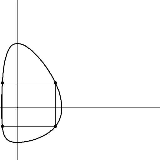
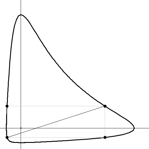
Refer to caption
Refer to caption
Figure 11: DD-spheres with respect to separable distances shown with a random box tangent at its vertices: To plot a DD-sphere, we only need to know the parametric equations on two opposite orthants to deduce the other orthants.

We now illustrate how to get the parametric equations of relative entropic spheres defined with respect to the Kullback-Leibler divergence and the Itakura-Saito divergence in terms of the branches of the Lambert W function [8].

2.5.1 Parameterization of the Kullback-Leibler spheres

The scalar extended Kullback-Leibler divergence defined on ℝ+\mathbb{R}^{+} is defined by:

DKL[θc:θ]:=θclogθcθ+θ−θc.D_{\mathrm{KL}}[\theta_{c}:\theta]:=\theta_{c}\log\frac{\theta_{c}}{\theta}+\theta-\theta_{c}.

The two solutions of this equation will rely on two branches of the Lambert W function [8]. Indeed, the equation x​ex=axe^{x}=a solves as

x={W0​(a)if a≥1eW−1​(a)if −1e≤a<0x=\left\{\begin{array}[]{ll}W_{0}(a)&\mbox{if $a\geq\frac{1}{e}$}\\ W_{-1}(a)&\mbox{if $-\frac{1}{e}\leq a<0$}\end{array}\right.

To solve DKL[θc:θ]=uD_{\mathrm{KL}}[\theta_{c}:\theta]=u for θc∈(0,1)\theta_{c}\in(0,1) and u≥0u\geq 0 amounts to solve the equation

θc​log⁡θcθ+θ\displaystyle\theta_{c}\log\frac{\theta_{c}}{\theta}+\theta =\displaystyle= u+θc,\displaystyle u+\theta_{c},
θ−θc​log⁡θ\displaystyle\theta-\theta_{c}\log\theta =\displaystyle= u+θc​(1−log⁡θc).\displaystyle u+\theta_{c}(1-\log\theta_{c}).

We get the two solutions using the two branches W0W_{0} and W−1W_{-1} of the Lambert W function [8]:

xDKL,θc,u;−1\displaystyle x_{D_{\mathrm{KL}},\theta_{c},u;-1} =\displaystyle= −θc​W0​(−exp⁡(−uθc−1)),\displaystyle-\theta_{c}W_{0}\left(-\exp\left(-\frac{u}{\theta_{c}}-1\right)\right), (120)
xDKL,θc,u;1\displaystyle x_{D_{\mathrm{KL}},\theta_{c},u;1} =\displaystyle= −θc​W−1​(−exp⁡(−uθc−1)).\displaystyle-\theta_{c}W_{-1}\left(-\exp\left(-\frac{u}{\theta_{c}}-1\right)\right). (121)

Figure 12 displays a DKLD_{\mathrm{KL}} sphere in two dimensions by plotting the four quadrant parameterizations. See the corresponding online video.77 7 https://www.youtube.com/watch?v=pgDwWJ1DQFY The restriction of the KL sphere to the hyperplane ∑i=1dθi=1\sum_{i=1}^{d}\theta^{i}=1 yields a Kullback-Leibler sphere on the (d−1)(d-1)-dimensional probability simplex (i.e., standard simplex) embedded in ℝd\mathbb{R}^{d}.

Figure 12: Plotting the parametric equations on each quadrant of an extented Kullback-Leibler circle sphereDKL​((12,12),12)\mathrm{sphere}_{D_{\mathrm{KL}}}((\frac{1}{2},\frac{1}{2}),\frac{1}{2}) on the plane. The first two plots show some inscribed isorectangles tangent at its four vertices to the extented Kullback-Leibler circle.

Figure 13 displays the four parameterized curves of the extended Kullback-Leibler circle.

Refer to caption
Figure 13: Quadrant-based parameterized curves of the extended Kullback-Leibler circle.

2.6 Parameterization of the Itakura-Saito spheres

The scalar Itakura-Saito divergence defined on ℝ+\mathbb{R}^{+} is

DIS[θc:θ]=θcθ−logθcθ−1.D_{\mathrm{IS}}[\theta_{c}:\theta]=\frac{\theta_{c}}{\theta}-\log\frac{\theta_{c}}{\theta}-1.

The Itakura-Saito divergence is a Bregman divergence for the generator F⁡(x)=−log⁡uF(x)=-\log u, and can thus be interpreted as a relative entropy.

For the Itakura-Saito divergence, we have to solve the following equation:

θcθ−log⁡(θcθ)−1=u.\frac{\theta_{c}}{\theta}-\log\left(\frac{\theta_{c}}{\theta}\right)-1=u.

Since θcθ=log⁡exp⁡(θcθ)\frac{\theta_{c}}{\theta}=\log\exp(\frac{\theta_{c}}{\theta}), we get:

xDIS,θc,u;−1\displaystyle x_{D_{\mathrm{IS}},\theta_{c},u;-1} =\displaystyle= −cxW−1​(−e−u−1),\displaystyle-\frac{c_{x}}{W_{-1}(-e^{-u-1})}, (122)
xDIS,θc,u;1\displaystyle x_{D_{\mathrm{IS}},\theta_{c},u;1} =\displaystyle= −cxW0​(−e−u−1).\displaystyle-\frac{c_{x}}{W_{0}(-e^{-u-1})}. (123)
Figure 14: Plotting the parametric equations on each quadrant of a Itakura-Saito circle sphereDIS​((12,12),1)\mathrm{sphere}_{D_{\mathrm{IS}}}((\frac{1}{2},\frac{1}{2}),1) on the plane. The first two plots show some inscribed isorectangles tangent at its four corners to the IS sphere.

Figure 14 displays a DISD_{\mathrm{IS}} sphere in two dimensions by plotting the four quadrant parameterizations. See the corresponding online video.88 8 https://www.youtube.com/watch?v=b4eJu1TT-to

Figure 15 displays the four parameterized curves of the Itakura-Saito circle.

Refer to caption
Figure 15: Quadrant-based parameterized curves of the extended Itakura-Saito circle.

Figure 16 visualizes and compares the parametric equations on a quadrant of the extended Kullback-Leibler circle and the Itakura-Saito circle.

Refer to caption
Figure 16: Parametric equations of the extended Kullback-Leibler circle and the Itakura-Saito circle on a quadrant (green part).

3 Geodesic ∇\nabla-triangles with one, two, or three interior right angles

3.1 Geodesic ∇\nabla-triangles with one interior right angle

To build a geodesic ∇\nabla-triangle with a right angle, fix two points pp and qq (i.e., the first two triangle vertices), and consider the location of the third triangle vertex point rr such that γq​r⟂qγq​p\gamma_{qr}\perp_{q}\gamma_{qp} (i.e., γ˙q​r(0)⟂qγ˙q​p(0)\dot{\gamma}_{qr}(0)\perp_{q}\dot{\gamma}_{qp}(0)). We end up with the following linear equation which defines a θ\theta-flat HqθH_{q}^{\theta}:

Hqθ:θr⊤​∇2F​(θq)​θp​q=θq⊤​∇2F​(θq)​θp​q.H_{q}^{\theta}:\theta_{r}^{\top}\nabla^{2}F(\theta_{q})\theta_{pq}=\theta_{q}^{\top}\nabla^{2}F(\theta_{q})\theta_{pq}. (124)

By restricting the solution r∈Hqθr\in H_{q}^{\theta} to the manifold MM, we get:

Proposition 1

The locii of points rr of a ∇\nabla-triangle that form a right angle at qq is Hqθ∩MH^{\theta}_{q}\cap M.

θ\theta η\eta
Figure 17: An example of a geodesic ∇\nabla-triangle with a right angle at qq: (thicker vertex is rr).

Figure 17 displays that a ∇\nabla-triangle with one right angle αq​(r,p)=π2\alpha_{q}(r,p)=\frac{\pi}{2} in the Itakura-Saito manifold: θ⁡(p)=(1.2885253880864789,3.4136709176658546)\theta(p)=(1.2885253880864789,3.4136709176658546),
θ⁡(q)=(4.9336774965526065,1.656631440605195)\theta(q)=(4.9336774965526065,1.656631440605195),
θ⁡(r)=(3.5399193730133236,4.6263857851449846)\theta(r)=(3.5399193730133236,4.6263857851449846).
The interior angles of the ∇\nabla-triangle are αp​(q,r)=1.8276508176456936\alpha_{p}(q,r)=1.8276508176456936,
αq​(p,r)=1.5707963267948966\alpha_{q}(p,r)=1.5707963267948966
and αr​(p,q)=1.1542328404967954\alpha_{r}(p,q)=1.1542328404967954.
That total sum of the interior angles are 4.5526799849373854.552679984937385 radians (equivalent to about 260.8260.8 degrees).

3.2 Geodesic ∇\nabla-triangles with two interior right angles

We now report the construction of two right angle ∇\nabla-triangles. That is, geodesic triangles with all primal geodesic edges (i.e., ∇\nabla-triangle), with both the right angles αp​(q,r)=90o\alpha_{p}(q,r)=90^{o} and αq​(p,r)=90o\alpha_{q}(p,r)=90^{o}. Figure 18 displays such a double right angle ∇\nabla-triangle for the Burg negentropy generator FIS​(θ)F_{\mathrm{IS}}(\theta) yielding the Itakura-Saito divergence. Observe that because the metric tensor field gg is not a scalar function of the Euclidean metric tensor gEucg_{\mathrm{Euc}}, the Itakura-Saito Bregman geometry is not conformal (see Figure 5).

Refer to caption
Figure 18: An example of double right angle ∇\nabla-triangle visualized in the primal θ\theta-coordinate system for the Itakura-Saito Bregman manifold.

Now, fix two points pp and qq, and let us seek for the third point rr of the ∇\nabla-triangle γp​q​γq​r​γr​p\gamma_{pq}\gamma_{qr}\gamma_{rp} such that it holds both simultaneously that (i) γq​r⟂qγq​p\gamma_{qr}\perp_{q}\gamma_{qp} (i.e., γ˙q​r(0)⟂qγ˙q​p(0)\dot{\gamma}_{qr}(0)\perp_{q}\dot{\gamma}_{qp}(0)) and (ii) γp​q⟂pγp​r\gamma_{pq}\perp_{p}\gamma_{pr} (i.e., γ˙p​q(0)⟂pγ˙p​r(0)\dot{\gamma}_{pq}(0)\perp_{p}\dot{\gamma}_{pr}(0)). We end up with the following system of equations:

{θr⊤​∇2F​(θq)​θp​q=θq⊤​∇2F​(θq)​θp​q,θr⊤​∇2F​(θp)​θp​q=θp⊤​∇2F​(θp)​θp​q.\left\{\begin{array}[]{lcl}\theta_{r}^{\top}\nabla^{2}F(\theta_{q})\theta_{pq}&=&\theta_{q}^{\top}\nabla^{2}F(\theta_{q})\theta_{pq},\\ \theta_{r}^{\top}\nabla^{2}F(\theta_{p})\theta_{pq}&=&\theta_{p}^{\top}\nabla^{2}F(\theta_{p})\theta_{pq}.\end{array}\right. (125)

It is a linear system A​θ=bA\theta=b with

A=[ai​j]=[∇2F​(θq)​θp​q∇2F​(θp)​θp​q],b=[bi]=[θq⊤​∇2F​(θq)​θp​qθp⊤​∇2F​(θp)​θp​q].A=[a_{ij}]=\left[\begin{array}[]{l}\nabla^{2}F(\theta_{q})\theta_{pq}\cr\nabla^{2}F(\theta_{p})\theta_{pq}\end{array}\right],\quad b=[b_{i}]=\left[\begin{array}[]{l}\theta_{q}^{\top}\nabla^{2}F(\theta_{q})\theta_{pq}\cr\theta_{p}^{\top}\nabla^{2}F(\theta_{p})\theta_{pq}\end{array}\right]. (126)

When ∇2F​(θ)=Q≻0\nabla^{2}F(\theta)=Q\succ 0 for a fixed positive-definite matrix and p≠qp\not=q, the system does not admit any solution (i.e., case of squared Mahalanobis distances which generalize the squared Euclidean distance and can have at most one right angle).

Otherwise, this linear system solves uniquely for asymmetric Bregman divergences [6] using Cramer’s rule as

θr1=|b1a12b2a22||A|,θr2=|a11b1a21b2||A|,\theta_{r}^{1}=\frac{\left|\begin{array}[]{ll}b_{1}&a_{12}\cr b_{2}&a_{22}\end{array}\right|}{|A|},\quad\theta_{r}^{2}=\frac{\left|\begin{array}[]{ll}a_{11}&b_{1}\cr a_{21}&b_{2}\end{array}\right|}{|A|}, (127)

where |⋅||\cdot| denotes the matrix determinant.

θ\theta η\eta
θ\theta η\eta
Figure 19: Two examples of ∇\nabla-triangles with two interior right angles (the opposite angles to the thicker vertex rr).

Similarly, we can build ∇∗\nabla^{*}-triangles with two right angles by exchanging F⇔F∗F\Leftrightarrow F^{*}. Notice that having two right angles in a non-degenerate triangle makes it necessarily having an angle excess.

Figure 19 displays the following two double right angle ∇\nabla-triangles (up to machine numerical precision) obtained for the following settings:

  • •

    θ⁡(p)=(1.7372662352145616,1.148396070619242)\theta(p)=(1.7372662352145616,1.148396070619242),
    θ⁡(q)=(1.241571556333764,1.3768479188317202)\theta(q)=(1.241571556333764,1.3768479188317202),
    θ⁡(r)=(1.614143828700357,1.8451358255393877)\theta(r)=(1.614143828700357,1.8451358255393877),
    αp​(q,r)=90.00000000000001\alpha_{p}(q,r)=90.00000000000001,
    αq​(p,r)=90.0\alpha_{q}(p,r)=90.0,
    αr​(p,q)=12.82764159141668\alpha_{r}(p,q)=12.82764159141668.

  • •

    θ⁡(p)=(1.7128340504770114,1.2510418358297621)\theta(p)=(1.7128340504770114,1.2510418358297621),
    θ⁡(q)=(1.446857135939727,1.7930125176801988)\theta(q)=(1.446857135939727,1.7930125176801988),
    θ⁡(r)=(1.1177842396781703,1.5922051785236535)\theta(r)=(1.1177842396781703,1.5922051785236535),
    αp​(q,r)=90.00000000000001\alpha_{p}(q,r)=90.00000000000001,
    αq​(p,r)=90.00000000000001\alpha_{q}(p,r)=90.00000000000001,
    αr​(p,q)=6.595093466701274\alpha_{r}(p,q)=6.595093466701274.

Define the following two θ\theta-flat submanifolds:

Hqθ\displaystyle H^{\theta}_{q} :\displaystyle: θr⊤​∇2F​(θq)​θp​q−θq⊤​∇2F​(θq)​θp​q=0,\displaystyle\theta_{r}^{\top}\nabla^{2}F(\theta_{q})\theta_{pq}-\theta_{q}^{\top}\nabla^{2}F(\theta_{q})\theta_{pq}=0, (128)
Hpθ\displaystyle H^{\theta}_{p} :\displaystyle: θr⊤​∇2F​(θp)​θp​q−θp⊤​∇2F​(θp)​θp​q=0.\displaystyle\theta_{r}^{\top}\nabla^{2}F(\theta_{p})\theta_{pq}-\theta_{p}^{\top}\nabla^{2}F(\theta_{p})\theta_{pq}=0. (129)

We end up with the following proposition:

Proposition 2

In a non-Mahalanobis Bregman manifold MM, the locii of points rr that form a double right angle with the geodesic arc γp​q\gamma_{pq} is Hqθ∩HqθH^{\theta}_{q}\cap H^{\theta}_{q}.

Remember that the intersection of θ\theta-flats is a θ\theta-flat.

Notice that if instead of constraining two interior angles of a ∇\nabla-triangle to have right angles, we ask for two prescribed angles αq​(p,r)\alpha_{q}(p,r) and αp​(q,r)\alpha_{p}(q,r), we would end up with the following system of non-linear equations to solve:

{θr​q⊤​∇2F​(θq)​θp​q=∥θr​q∥∇2F​(θq)∥θp​q∥∇2F​(θq)cosαq(p,r),θr​q⊤​∇2F​(θp)​θp​q=∥θr​q|∇2F​(θp)∥θp​q|∇2F​(θp)cosαp(q,r).\left\{\begin{array}[]{lcl}\theta_{rq}^{\top}\nabla^{2}F(\theta_{q})\theta_{pq}&=&\|\theta_{rq}\|_{\nabla^{2}F(\theta_{q})}\|\theta_{pq}\|_{\nabla^{2}F(\theta_{q})}\cos\alpha_{q}(p,r),\\ \theta_{rq}^{\top}\nabla^{2}F(\theta_{p})\theta_{pq}&=&\|\theta_{rq}|_{\nabla^{2}F(\theta_{p})}\|\theta_{pq}|_{\nabla^{2}F(\theta_{p})}\cos\alpha_{p}(q,r).\end{array}\right. (130)

Solving this non-linear system for rr gives a solution whenever the system is feasible.

3.3 Geodesic ∇\nabla-triangles with three interior right angles

Given a triple of points (p,q,r)(p,q,r), we may consider two fundamental types of triangles (up to duality and point permutations): a ∇\nabla-triangle (type ppp) or a triangle of type p​d​ppdp.

Let us consider a geodesic ∇\nabla-triangle γp​q​γq​r​γr​p\gamma_{pq}\gamma_{qr}\gamma_{rp} so that it holds simultaneously:

γp​q⟂pγp​r,γq​r⟂qγq​p,γr​p⟂rγr​q.\gamma_{pq}\perp_{p}\gamma_{pr},\quad\gamma_{qr}\perp_{q}\gamma_{qp},\quad\gamma_{rp}\perp_{r}\gamma_{rq}. (131)

Writing the above constraints in the primal θ\theta-coordinate system, we end up with the following system to solve:

{θq​p⊤​∇2F​(θp)​θr​p=0θr​q⊤​∇2F​(θq)​θp​q=0θp​r⊤​∇2F​(θr)​θq​r=0.\left\{\begin{array}[]{lcl}\theta_{qp}^{\top}\nabla^{2}F(\theta_{p})\theta_{rp}&=&0\\ \theta_{rq}^{\top}\nabla^{2}F(\theta_{q})\theta_{pq}&=&0\\ \theta_{pr}^{\top}\nabla^{2}F(\theta_{r})\theta_{qr}&=&0.\end{array}\right. (132)

Because of the Hessian matrices, this yields in general a non-linear system of equations to solve. The set of feasible solutions define the ∇\nabla-triangles with three right angles. In dimension DD, we have 3D unknown (the DD θ\theta-coordinates of the points pp, qq, and rr) for 33 constraints. That is, the system is underconstrained.

For the 2D Itakura-Saito manifold, the Hessian matrix at pp is diag⁡(1sqr⁡(θx),1sqr⁡(θy))\mathrm{diag}\left(\frac{1}{\mathrm{sqr}(\theta_{x})},\frac{1}{\mathrm{sqr}(\theta_{y})}\right). Thus we get the following system to solve:

(θqx−θpx)​1sqr⁡(θpx)​(θrx−θpx)+(θqy−θpy)​1sqr⁡(θpy)​(θry−θpy)\displaystyle(\theta_{q}^{x}-\theta_{p}^{x})\frac{1}{\mathrm{sqr}(\theta_{p}^{x})}(\theta_{r}^{x}-\theta_{p}^{x})+(\theta_{q}^{y}-\theta_{p}^{y})\frac{1}{\mathrm{sqr}(\theta_{p}^{y})}(\theta_{r}^{y}-\theta_{p}^{y}) =\displaystyle= 0,\displaystyle 0, (133)
(θrx−θqx)​1sqr⁡(θqx)​(θpx−θqx)+(θry−θqy)​1sqr⁡(θqy)​(θpy−θqy)\displaystyle(\theta_{r}^{x}-\theta_{q}^{x})\frac{1}{\mathrm{sqr}(\theta_{q}^{x})}(\theta_{p}^{x}-\theta_{q}^{x})+(\theta_{r}^{y}-\theta_{q}^{y})\frac{1}{\mathrm{sqr}(\theta_{q}^{y})}(\theta_{p}^{y}-\theta_{q}^{y}) =\displaystyle= 0,\displaystyle 0, (134)
(θpx−θrx)​1sqr⁡(θrx)​(θqx−θrx)+(θpy−θry)​1sqr⁡(θry)​(θqy−θry)\displaystyle(\theta_{p}^{x}-\theta_{r}^{x})\frac{1}{\mathrm{sqr}(\theta_{r}^{x})}(\theta_{q}^{x}-\theta_{r}^{x})+(\theta_{p}^{y}-\theta_{r}^{y})\frac{1}{\mathrm{sqr}(\theta_{r}^{y})}(\theta_{q}^{y}-\theta_{r}^{y}) =\displaystyle= 0.\displaystyle 0. (135)

Multiplying Eq. 133 by sqr⁡(θpx)​sqr​(θpy)\mathrm{sqr}(\theta_{p}^{x})\mathrm{sqr}(\theta_{p}^{y}), Eq. 134 by sqr⁡(θqx)​sqr​(θqy)\mathrm{sqr}(\theta_{q}^{x})\mathrm{sqr}(\theta_{q}^{y}), and Eq. 135 by sqr⁡(θrx)​sqr​(θry)\mathrm{sqr}(\theta_{r}^{x})\mathrm{sqr}(\theta_{r}^{y}), we get a system of polynomial equations to solve [35]:

(θqx−θpx)​sqr​(θpy)​(θrx−θpx)+(θqy−θpy)​sqr​(θpx)​(θry−θpy)\displaystyle(\theta_{q}^{x}-\theta_{p}^{x})\mathrm{sqr}(\theta_{p}^{y})(\theta_{r}^{x}-\theta_{p}^{x})+(\theta_{q}^{y}-\theta_{p}^{y}){\mathrm{sqr}(\theta_{p}^{x})}(\theta_{r}^{y}-\theta_{p}^{y}) =\displaystyle= 0,\displaystyle 0, (137)
(θrx−θqx)​sqr​(θqy)​(θpx−θqx)+(θry−θqy)​sqr​(θqx)​(θpy−θqy)\displaystyle(\theta_{r}^{x}-\theta_{q}^{x}){\mathrm{sqr}(\theta_{q}^{y})}(\theta_{p}^{x}-\theta_{q}^{x})+(\theta_{r}^{y}-\theta_{q}^{y}){\mathrm{sqr}(\theta_{q}^{x})}(\theta_{p}^{y}-\theta_{q}^{y}) =\displaystyle= 0,\displaystyle 0, (138)
(θpx−θrx)​sqr​(θry)​(θqx−θrx)+(θpy−θry)​sqr​(θrx)​(θqy−θry)\displaystyle(\theta_{p}^{x}-\theta_{r}^{x}){\mathrm{sqr}(\theta_{r}^{y})}(\theta_{q}^{x}-\theta_{r}^{x})+(\theta_{p}^{y}-\theta_{r}^{y}){\mathrm{sqr}(\theta_{r}^{x})}(\theta_{q}^{y}-\theta_{r}^{y}) =\displaystyle= 0,\displaystyle 0, (139)

where sqr⁡(x)=x2\mathrm{sqr}(x)=x^{2}. The system of polynomial equations has 33 equations with 66 positive variables defining 33 pairs of distinct points (θpx,θpy)(\theta_{p}^{x},\theta_{p}^{y}), (θqx,θqy)(\theta_{q}^{x},\theta_{q}^{y}), and (θrx,θry)(\theta_{r}^{x},\theta_{r}^{y}).

When considering the extended Kullback-Leibler manifold, since the Hessian matrix at pp is diag⁡(1θpx,1θpy)\mathrm{diag}\left(\frac{1}{\theta_{p}^{x}},\frac{1}{\theta_{p}^{y}}\right), we get the following system of polynomial equations (after multiplying the first equation by θpx​θpy\theta_{p}^{x}\theta_{p}^{y}, the second equation by θqx​θqy\theta_{q}^{x}\theta_{q}^{y} and the third equation by θrx​θry\theta_{r}^{x}\theta_{r}^{y}):

{(θqx−θpx)​θpy​(θrx−θpx)+(θqy−θpy)​θpx​(θry−θpy)=0,(θrx−θqx)​θqy​(θpx−θqx)+(θry−θqy)​θqx​(θpy−θqy)=0,(θpx−θrx)​θry​(θqx−θrx)+(θpy−θry)​θrx​(θqy−θry)=0.\left\{\begin{array}[]{lcl}(\theta_{q}^{x}-\theta_{p}^{x})\theta_{p}^{y}(\theta_{r}^{x}-\theta_{p}^{x})+(\theta_{q}^{y}-\theta_{p}^{y})\theta_{p}^{x}(\theta_{r}^{y}-\theta_{p}^{y})&=&0,\\ (\theta_{r}^{x}-\theta_{q}^{x})\theta_{q}^{y}(\theta_{p}^{x}-\theta_{q}^{x})+(\theta_{r}^{y}-\theta_{q}^{y})\theta_{q}^{x}(\theta_{p}^{y}-\theta_{q}^{y})&=&0,\\ (\theta_{p}^{x}-\theta_{r}^{x})\theta_{r}^{y}(\theta_{q}^{x}-\theta_{r}^{x})+(\theta_{p}^{y}-\theta_{r}^{y})\theta_{r}^{x}(\theta_{q}^{y}-\theta_{r}^{y})&=&0.\end{array}\right. (140)

Fixing three variables, we get a cubic system of three equations in three unknowns.

We used Wolfram alpha™ to check for potential real solution(s) of the system:

a>0, b>0, c>a, x>0, y>c,z>0,
(c-a)*b*(y-a)+(x-b)*a*(z-b)=0,
(y-c)*x*(a-c)+(z-x)*c*(b-x)=0,
(a-y)*z*(c-y)+(b-z)*y*(x-z)=0

The system does not admit solution in the positive orthant. We also checked the feasibility of the system for the Itakura-Saito manifold:

a>0, b>0, c>a, x>0, y>c,z>0,
(c-a)*b*b*(y-a)+(x-b)*a*a*(z-b)=0,
(y-c)*x*x*(a-c)+(z-x)*c*c*(b-x)=0,
(a-y)*z*z*(c-y)+(b-z)*y*y*(x-z)=0.

The system does not admit solution in the positive orthant.

Thus it is an ongoing task to report an example of such a ∇\nabla-triangle with three right angles for an asymmetric Bregman divergence, or to prove that such a triangle can never exist.

4 Simultaneous satisfying the dual Pythagorean theorems

Fix two points pp and qq of the Bregman manifold MM. We seek for the locii of the third point r∈Mr\in M such that we have both γp​q⟂qγq​r∗\gamma_{pq}\perp_{q}\gamma_{qr}^{*} and γp​q∗⟂qγq​r\gamma_{pq}^{*}\perp_{q}\gamma_{qr}. That is, we need to solve the following system of equations:

{(η⁡(p)−η⁡(q))⊤​(θ⁡(r)−θ⁡(q))=0,(η⁡(p)−η⁡(q))⊤​(θ⁡(r)−θ⁡(q))=0.\left\{\begin{array}[]{lll}(\eta(p)-\eta(q))^{\top}(\theta(r)-\theta(q))&=&0,\cr(\eta(p)-\eta(q))^{\top}(\theta(r)-\theta(q))&=&0.\end{array}\right. (141)

Notice that finding such triples of points allow one to construct dual geodesic right-angle triangles. When F⁡(θ)=12​θ⊤​Q​θF(\theta)=\frac{1}{2}\theta^{\top}Q\theta for Q≻0Q\succ 0 a positive-definite matrix, we have BFB_{F} that is a squared Mahalanobis distances, and the primal and dual geodesics coincide. Therefore any right-angle triangle is a dually right-angle solution to the problem in Mahalanobis manifolds. Thus we shall consider asymmetric Bregman divergences in the remainder since the only symmetric Bregman divergences are squared Mahalanobis distances [6].

4.1 Simultaneous dual orthogonality: A geometric interpretation

The constraint γp​q⟂qγq​r∗\gamma_{pq}\perp_{q}\gamma_{qr}^{*} is equivalent to (θ⁡(p)−θ⁡(q))⊤​(η⁡(r)−η⁡(q))=0(\theta(p)-\theta(q))^{\top}(\eta(r)-\eta(q))=0. Let θp​q=θ⁡(p)−θ⁡(q)\theta_{pq}=\theta(p)-\theta(q), ηr=η⁡(r)\eta_{r}=\eta(r) and ηq=η⁡(q)\eta_{q}=\eta(q). Then we have the following affine equation in ηr\eta_{r}:

Hη​(p,q):θp​q⊤​ηr−θp​q⊤​ηq=0.H^{\eta}(p,q):\theta_{pq}^{\top}\eta_{r}-\theta_{pq}^{\top}\eta_{q}=0. (142)

The locii rr of points satisfying the above equation is a (D−1)(D-1)-dimensional ∇∗\nabla^{*}-autoparallel submanifold Hη​(p,q)H^{\eta}(p,q) (i.e., a (D−1)(D-1)-dimensional η\eta-flat [3] or loosely speaking a “∇∗\nabla^{*}-hyperplane”).

Similarly, the constraint γp​q∗⟂qγq​r\gamma_{pq}^{*}\perp_{q}\gamma_{qr} is equivalent to (η⁡(p)−η⁡(q))⊤​(θ⁡(r)−θ⁡(q))=0(\eta(p)-\eta(q))^{\top}(\theta(r)-\theta(q))=0. Let ηp​q=η⁡(p)−η⁡(q)\eta_{pq}=\eta(p)-\eta(q), θr=θ⁡(r)\theta_{r}=\theta(r) and θq=θ⁡(q)\theta_{q}=\theta(q). Then we have the following affine equation in θr\theta_{r}:

Hθ​(p,q):ηp​q⊤​θr−ηp​q⊤​θq=0.H^{\theta}(p,q):\eta_{pq}^{\top}\theta_{r}-\eta_{pq}^{\top}\theta_{q}=0. (143)

The locii rr of points satisfying the above equation is a (D−1)(D-1)-dimensional ∇\nabla-autoparallel submanifold Hθ​(p,q)H^{\theta}(p,q) (i.e., a (D−1)(D-1)-dimensional θ\theta-flat [3] or ∇\nabla-hyperplane).

Notice that point qq ought to belong to both Hη​(p,q)H^{\eta}(p,q) and Hθ​(p,q)H^{\theta}(p,q). Thus to simultaneously satisfy the two dual geodesic orthogonality constraints, the point rr should belong to the intersection of a η\eta-flat with a θ\theta-flat:

S⁡(p,q)=Hη​(p,q)∩Hθ​(p,q).S(p,q)=H^{\eta}(p,q)\cap H^{\theta}(p,q). (144)

We should make sure S⁡(p,q)S(p,q) belongs to the manifold MM when solving the equations using either the θ\theta- or η\eta-coordinate system.

Proposition 3

The locii of points rr such that γp​q⟂qγq​r∗\gamma_{pq}\perp_{q}\gamma_{qr}^{*} and γp​q∗⟂qγq​r\gamma_{pq}^{*}\perp_{q}\gamma_{qr} is the intersection of a θ\theta-flat with a η\eta-flat restricted to the manifold: S⁡(p,q)=Hη​(p,q)∩Hθ​(p,q)S(p,q)=H^{\eta}(p,q)\cap H^{\theta}(p,q).

In general the intersection of a θ\theta-flat with a η\eta-flat is neither a θ\theta-flat nor a η\eta-flat. In 2D, the submanifolds Hη​(p,q)H^{\eta}(p,q) and Hθ​(p,q)H^{\theta}(p,q) can be interpreted as a dual geodesic and a primal geodesic, respectively. Thus in 2D, Sp​qS_{pq} may not be simply connected, and the maximum number of points of the intersection of two geodesics upper bounds the number of solutions for rr. The next section illustrates how to build such triples of points for the Itakura-Saito manifold.

4.2 Explicit construction in the Itakura-Saito manifold

Consider the Itakura-Saito manifold described in §2.4.3. Let us exhibit some triple of points (p,q,r)(p,q,r) such that γp​q⟂qγq​r∗\gamma_{pq}\perp_{q}\gamma_{qr}^{*} and γp​q∗⟂qγq​r\gamma_{pq}^{*}\perp_{q}\gamma_{qr}. To avoid confusion, let us write the 2D θ\theta- and η\eta-coordinates of pp by θpx\theta_{p}^{x} and θpy\theta_{p}^{y}, and ηpx\eta_{p}^{x} and ηpy\eta_{p}^{y}.

The second orthogonality constraint equation yields the equation ηp​q⊤​(θr−θq)=ηp​qx​θrx+ηp​qy​θry−ηp​q⊤​θq=0\eta_{pq}^{\top}(\theta_{r}-\theta_{q})=\eta_{pq}^{x}\theta_{r}^{x}+\eta_{pq}^{y}\theta_{r}^{y}-\eta_{pq}^{\top}\theta_{q}=0 which can be rewritten as:

θry\displaystyle\theta_{r}^{y} =\displaystyle= −ηp​qxηp​qy​θrx+ηp​q⊤​θqηp​qy=a​θrx+b,\displaystyle-\frac{\eta_{pq}^{x}}{\eta_{pq}^{y}}\theta_{r}^{x}+\frac{\eta_{pq}^{\top}\theta_{q}}{\eta_{pq}^{y}}=a\theta_{r}^{x}+b, (145)

with a=−ηp​qxηp​qya=-\frac{\eta_{pq}^{x}}{\eta_{pq}^{y}} and b=ηp​q⊤​θqηp​qyb=\frac{\eta_{pq}^{\top}\theta_{q}}{\eta_{pq}^{y}}.

The first orthogonality constraint equation yields (θp​q)⊤​(ηr−ηq)(\theta_{pq})^{\top}(\eta_{r}-\eta_{q}) with ηrx=−1θrx\eta_{r}^{x}=-\frac{1}{\theta_{r}^{x}} and ηry=−1θry\eta_{r}^{y}=-\frac{1}{\theta_{r}^{y}}. After multiplying both sides of the equation by θrx​θry\theta_{r}^{x}\theta_{r}^{y}, we find

−θp​qx​θry−θp​qy​θrx−θp​q⊤​ηq​θrx​θry=0\displaystyle-\theta_{pq}^{x}\theta_{r}^{y}-\theta_{pq}^{y}\theta_{r}^{x}-\theta_{pq}^{\top}\eta_{q}\theta_{r}^{x}\theta_{r}^{y}=0 (146)
Figure 20: The intersection of Hη​(p,q)H^{\eta}(p,q) and Hθ​(p,q)H^{\theta}(p,q) (displayed in black) yields two points: point qq and the solution point rr.

Letting θry=a​θrx+b\theta_{r}^{y}=a\theta_{r}^{x}+b, we get the following quadratic equation to solve:

−θp​qx​(a​θrx+b)−θp​qy​θrx−θp​q⊤​ηq​θrx​(a​θrx+b)=0.\displaystyle-\theta_{pq}^{x}(a\theta_{r}^{x}+b)-\theta_{pq}^{y}\theta_{r}^{x}-\theta_{pq}^{\top}\eta_{q}\theta_{r}^{x}(a\theta_{r}^{x}+b)=0. (147)

We write the former equation into the following canonical form of quadratic equations:

(−θp​q⊤​ηq​a)⏟A​(θrx)2+(−θp​qx​a−θp​qy−b​θp​q⊤​ηq)⏟B​θrx+(−θp​qx​b)⏟C=0.\displaystyle\underbrace{(-\theta_{pq}^{\top}\eta_{q}a)}_{A}(\theta_{r}^{x})^{2}+\underbrace{(-\theta_{pq}^{x}a-\theta_{pq}^{y}-b\theta_{pq}^{\top}\eta_{q})}_{B}\theta_{r}^{x}+\underbrace{(-\theta_{pq}^{x}b)}_{C}=0. (148)

Then we solve the quadratic equation, and get the two solutions: Let Δ=B2−4​A​C>0\Delta=B^{2}-4AC>0 be the discriminant. We have the two quadratic roots: θrx=−B−Δ2​A{\theta_{r}^{x}}=\frac{-B-\sqrt{\Delta}}{2A} and θrx′′=−B+Δ2​A{\theta_{r}^{x}}^{\prime\prime}=\frac{-B+\sqrt{\Delta}}{2A}, and we recover θry′=a​θrx′+b{\theta_{r}^{y}}^{\prime}=a{\theta_{r}^{x}}^{\prime}+b and θry′′=a​θrx′′+b{\theta_{r}^{y}}^{\prime\prime}=a{\theta_{r}^{x}}^{\prime\prime}+b. One of the two solutions r′r^{\prime} or r′′r^{\prime\prime} coincide with point qq (with coordinate θ⁡(q)\theta(q)), so the solution point rr is the remaining distinct point.

Figure 20 displays an example of a triple (p,q,r)(p,q,r) with doubly right-angle at qq with the pair of constraints Hη​(p,q)H^{\eta}(p,q) and Hη​(p,q)H^{\eta}(p,q) passing through point qq.

Let us give a numerical example. Set
θ⁡(p)=(θpx,θpy)=(0.7273955397832663,0.3279475469672596)\theta(p)=(\theta_{p}^{x},\theta_{p}^{y})=(0.7273955397832663,0.3279475469672596),
θ⁡(q)=(θqx,θqy)=(0.46251884248040354,0.3902872167636309)\theta(q)=(\theta_{q}^{x},\theta_{q}^{y})=(0.46251884248040354,0.3902872167636309). Then we solve the quadratic equation and find the two solutions
θ⁡(r)=(0.3065847355580658,0.13822426240588664)\theta(r)=(0.3065847355580658,0.13822426240588664)
and
θ⁡(r′′)=(0.4625188424804033,0.39028721676363043)\theta(r^{\prime\prime})=(0.4625188424804033,0.39028721676363043).
Observe that r′′=qr^{\prime\prime}=q so that the solution is r=r′r=r^{\prime}. The triple (p,q,r′)(p,q,r^{\prime}) holds simultaneously the dual Pythagorean theorems at point qq.

Figure 21 displays three examples of triples of points for which the dual Pythagorean theorems hold simultaneously. The triples of points displayed in Figure 21 are from left to right:

  1. 1.

    θ⁡(p)=(0.9704854205553236,1.4760141668100146)\theta(p)=(0.9704854205553236,1.4760141668100146),
    θ⁡(q)=(1.141690604206171,0.43035569351200803)\theta(q)=(1.141690604206171,0.43035569351200803) and
    θ⁡(r)=(0.22647618241885010.34444830042268043)\theta(r)=(0.22647618241885010.34444830042268043).

  2. 2.

    θ⁡(p)=(1.3163859900481611,1.965380252548788)\theta(p)=(1.3163859900481611,1.965380252548788),
    θ⁡(q)=(1.5136826962585432,1.2440688670072433)\theta(q)=(1.5136826962585432,1.2440688670072433) and
    θ⁡(r)=(0.6359397574807304,0.9494657726625966)\theta(r)=(0.6359397574807304,0.9494657726625966).

  3. 3.

    θ⁡(p)=(0.9511702030611633,1.291145089053253)\theta(p)=(0.9511702030611633,1.291145089053253),
    θ⁡(q)=(0.3277859642409383,1.906447912395776)\theta(q)=(0.3277859642409383,1.906447912395776) and
    θ⁡(r)=(0.1077217190919158,0.14622448026891943)\theta(r)=(0.1077217190919158,0.14622448026891943).

Figure 21: Three examples of triples of points (p,q,r)(p,q,r) visualized in the θ\theta-coordinate system for which the dual Pythagorean theorems hold simultaneously at qq for the Burg negentropy generator. That is, we have both γp​q⟂qγq​r∗\gamma_{pq}\perp_{q}\gamma_{qr}^{*} and γp​q∗⟂qγq​r\gamma_{pq}^{*}\perp_{q}\gamma_{qr}: The two pairs of (red,blue) geodesics form a right-angle at qq: A “doubly right-angle”.

From these two pairs of dual right angle geodesic arcs at qq, we can obtain four geodesic triangles by choosing either the primal or dual geodesic edge for the triangle edge p​qpq: Namely, γp​q​γq​r​γr​p∗\gamma_{pq}\gamma_{qr}\gamma_{rp}^{*}, γp​q∗​γq​r​γr​p∗\gamma_{pq}^{*}\gamma_{qr}\gamma_{rp}^{*} and γp​q​γq​r∗​γr​p\gamma_{pq}\gamma_{qr}^{*}\gamma_{rp}, γp​q∗​γq​r∗​γr​p\gamma_{pq}^{*}\gamma_{qr}^{*}\gamma_{rp}. These four triangles can be grouped into two dual pairs of dual geodesic triangles which exhibit a dually right angle at vertex qq: (γp​q​γq​r​γr​p∗,γp​q∗​γq​r∗​γr​p)(\gamma_{pq}\gamma_{qr}\gamma_{rp}^{*},\gamma_{pq}^{*}\gamma_{qr}^{*}\gamma_{rp}) and (γp​q∗​γq​r​γr​p∗,γp​q​γq​r∗​γr​p)(\gamma_{pq}^{*}\gamma_{qr}\gamma_{rp}^{*},\gamma_{pq}\gamma_{qr}^{*}\gamma_{rp}).

Similarly, solving the dual orthogonality constraint at qq for the cubic generator F⁡(θ)=13​∑iθi3F(\theta)=\frac{1}{3}\sum_{i}\theta_{i}^{3} yields a quadratic equation to solve. However, when considering the extended Shannon negentropy generator F⁡(θ)=∑i=1Dθi​log⁡θi−θiF(\theta)=\sum_{i=1}^{D}\theta^{i}\log\theta^{i}-\theta^{i}, we get a nonlinear equation (with sum of logarithmic terms) to solve: In 1D, we can easily run numerical optimization to approximate a solution numerically.

5 Conclusion

In a dually flat space [3] that we called a Bregman manifold in §2, geodesic triangles can either have angle excesses or angle defects like in arbitrary Riemannian geometry when the manifold is non self-dual (i.e., not of type Mahalanobis). First, we explained in §3 how to build geodesic ∇\nabla-triangles with one, two or three right angles provided that the corresponding system of equations is feasible. The system of equations is linear up to two right angles but non-linear when dealing with three right angles. Second, we showed how to build triple of points (p,q,r)(p,q,r) such that the dual Pythagorean theorems hold simultaneously at point qq yielding a dually right angle at qq: two dual pairs of right-angle dual geodesics. It turned out that the locii of such points rr for given points pp and qq is the intersection of a η\eta-flat with a θ\theta-flat. We reported the explicit construction of such triples for the Itakura-Saito manifold in §4.2.

In future work, we shall consider dually flat spaces for symmetric positive-definite matrices [30, 22, 2] where the inner product is the trace of a matrix product. We would also like to prove the following experimental observation: For the 2D Burg negentropy generator, the total sum α⁡(T)\alpha(T) of the interior angles of a geodesic ∇\nabla-triangle (geodesic triangle with all primal edges) plus the total sum β=α⁡(T∗)\beta=\alpha(T^{*}) of the interior angles of a dual geodesic ∇∗\nabla^{*}-triangle (geodesic triangle with all dual geodesic edges) sum up to 2​π2\pi. For example, for θ⁡(p)=(0.5,0.5)\theta(p)=(0.5,0.5), θ⁡(q)=(0.75,0.75)\theta(q)=(0.75,0.75) and θ⁡(r)=(0.95,0.25)\theta(r)=(0.95,0.25), we find that α⁡(T)=160.19318300825412o\alpha(T)=160.19318300825412^{o} (angle defect), β=α⁡(T∗)=199.80681699174588o\beta=\alpha(T^{*})=199.80681699174588^{o} (angle excess), and α+β=360.0o\alpha+\beta=360.0^{o}. This property seems only to hold for the 2D Itakura-Saito divergence and not in higher dimensions.

We shall also consider an extension of this work to study properties of geodesic convex kk-gons instead of geodesic triangles (i.e., 33-gons) in dually flat spaces (2k2^{k} such geodesic kk-gons). For example, the Lambert quadrilaterals [32] (i.e., 44-gons) have three right angles and the remaining angle which is acute in hyperbolic geometry, obtuse in spherical geometry, and a right angle in Euclidean geometry. In a dually flat space, we have 24=162^{4}=16 types of quadrilaterals defining overall 4×4=164\times 4=16 interior angles.99 9 A each quadrilateral vertex, we have 44 geodesics defining 66 interior angles between them. Figure 22 displays all pairs of dual geodesics of some convex quadrilaterals in the θ\theta- and η\eta-coordinate systems.

θ\theta-coordinate system η\eta-coordinate system
Figure 22: Examples of convex quadrangles in the Itakura-Saito manifold.

Acknowledgments: Figures were programmed using processing.org

References

  • [1] Shotaro Akaho, Hideitsu Hino, and Noboru Murata. On a convergence property of a geometrical algorithm for statistical manifolds. arXiv:1909.12644, 2019.
  • [2] Shun-ichi Amari. Information geometry of positive measures and positive-definite matrices: Decomposable dually flat structure. Entropy, 16(4):2131–2145, 2014.
  • [3] Shun-ichi Amari. Information geometry and its applications, volume 194. Springer, 2016.
  • [4] Katy S Azoury and Manfred K Warmuth. Relative loss bounds for on-line density estimation with the exponential family of distributions. Machine Learning, 43(3):211–246, 2001.
  • [5] Arindam Banerjee, Srujana Merugu, Inderjit S Dhillon, and Joydeep Ghosh. Clustering with Bregman divergences. Journal of machine learning research, 6(Oct):1705–1749, 2005.
  • [6] Jean-Daniel Boissonnat, Frank Nielsen, and Richard Nock. Bregman Voronoi diagrams. Discrete & Computational Geometry, 44(2):281–307, 2010.
  • [7] Lev M. Bregman. The relaxation method of finding the common point of convex sets and its application to the solution of problems in convex programming. USSR computational mathematics and mathematical physics, 7(3):200–217, 1967.
  • [8] Robert M Corless, Gaston H Gonnet, David EG Hare, David J Jeffrey, and Donald E Knuth. On the Lambert W function. Advances in Computational mathematics, 5(1):329–359, 1996.
  • [9] Jean-Pierre Crouzeix. A relationship between the second derivatives of a convex function and of its conjugate. Mathematical Programming, 13(1):364–365, 1977.
  • [10] Imre Csiszár. Information-type measures of difference of probability distributions and indirect observation. studia scientiarum Mathematicarum Hungarica, 2:229–318, 1967.
  • [11] Stephen Della Pietra, Vincent Della Pietra, and John Lafferty. Inducing features of random fields. IEEE transactions on pattern analysis and machine intelligence, 19(4):380–393, 1997.
  • [12] Herbert Edelsbrunner and Hubert Wagner. Topological data analysis with Bregman divergences. In 33rd International Symposium on Computational Geometry (SoCG 2017). Schloss Dagstuhl-Leibniz-Zentrum fuer Informatik, 2017.
  • [13] Shinto Eguchi et al. Geometry of minimum contrast. Hiroshima Mathematical Journal, 22(3):631–647, 1992.
  • [14] Luther Pfahler Eisenhart. Riemannian geometry. Princeton university press, 1997.
  • [15] Takashi Kurose. Dual connections and affine geometry. Mathematische Zeitschrift, 203(1):115–121, 1990.
  • [16] Stefan L. Lauritzen. Statistical manifolds. Differential geometry in statistical inference, 10:163–216, 1987.
  • [17] Prasanta Chandra Mahalanobis. On the generalized distance in statistics. Proceedings of the National Institute of Sciences (Calcutta), 2:49–55, 1936.
  • [18] Frank Nielsen. Legendre transformation and information geometry, 2010.
  • [19] Frank Nielsen. Cramér-Rao lower bound and information geometry. In Connected at Infinity II, pages 18–37. Springer, 2013.
  • [20] Frank Nielsen. An elementary introduction to information geometry. arXiv:1808.08271, 2018.
  • [21] Frank Nielsen. On geodesic triangles with right angles in a dually flat space. Progress in Information Geometry: Theory and Applications, pages 153–190191, 2021.
  • [22] Frank Nielsen and Rajendra Bhatia. Matrix information geometry. Springer, 2013.
  • [23] Frank Nielsen and Sylvain Boltz. The Burbea-Rao and Bhattacharyya centroids. IEEE Transactions on Information Theory, 57(8):5455–5466, 2011.
  • [24] Frank Nielsen and Vincent Garcia. Statistical exponential families: A digest with flash cards. arXiv:0911.4863, 2009.
  • [25] Frank Nielsen and Gaëtan Hadjeres. Monte Carlo information geometry: The dually flat case. arXiv preprint arXiv:1803.07225, 2018.
  • [26] Frank Nielsen, Boris Muzellec, and Richard Nock. Classification with mixtures of curved Mahalanobis metrics. In 2016 IEEE International Conference on Image Processing (ICIP), pages 241–245. IEEE, 2016.
  • [27] Frank Nielsen and Richard Nock. Sided and symmetrized Bregman centroids. IEEE transactions on Information Theory, 55(6):2882–2904, 2009.
  • [28] Frank Nielsen and Richard Nock. Skew Jensen-Bregman voronoi diagrams. In Transactions on Computational Science XIV, pages 102–128. Springer, 2011.
  • [29] Frank Nielsen and Richard Nock. On the geometry of mixtures of prescribed distributions. In IEEE International Conference on Acoustics, Speech and Signal Processing (ICASSP), pages 2861–2865. IEEE, 2018.
  • [30] Richard Nock, Brice Magdalou, Eric Briys, and Frank Nielsen. Mining matrix data with Bregman matrix divergences for portfolio selection. In Matrix Information Geometry, pages 373–402. Springer, 2013.
  • [31] Aleksandr Petrovich Norden. On pairs of conjugate parallel displacements in multidimensional spaces. Dokl. Akad. Nauk SSSR, 49(9):1345–1347, 1945.
  • [32] Boris A. Rosenfeld. A history of non-Euclidean geometry: Evolution of the concept of a geometric space, volume 12. Springer Science & Business Media, 2012.
  • [33] R. N. Sen. Parallel displacement and scalar product of vectors. In Proceedings of the National Institute of Sciences of India, volume 14, page 45. National Institute of Sciences of India, 1948.
  • [34] Hirohiko Shima. The geometry of Hessian structures. World Scientific, 2007.
  • [35] Bernd Sturmfels. Solving systems of polynomial equations. American Mathematical Soc., 2002. 97.
  • [36] Joseph Albert Wolf. Spaces of constant curvature, volume 372. American Mathematical Soc., 1972.
  • [37] Ting-Kam Leonard Wong. Logarithmic divergences from optimal transport and Rényi geometry. Information Geometry, 1(1):39–78, 2018.

Appendix A Notations

FF Strictly convex and C3C^{3} real-valued function
F∗F^{*} Dual Legendre-Fenchel convex conjugate
θ⁡(p)=(θ1​(p),…,θD​(p))\theta(p)=(\theta^{1}(p),\ldots,\theta^{D}(p)) primal coordinates of point pp
η⁡(p)=(η1​(p),…,ηD​(p))\eta(p)=(\eta_{1}(p),\ldots,\eta_{D}(p)) dual coordinates of point pp
θa​b=θa−θb\theta_{ab}=\theta_{a}-\theta_{b} notational shortcut
ηa​b=ηa−ηb\eta_{ab}=\eta_{a}-\eta_{b} notational shortcut
DF​(p:q)D_{F}(p:q) Divergence between points
BF​(θ⁡(p):θ⁡(q))B_{F}(\theta(p):\theta(q)) Bregman divergence
AF​(θ⁡(p):η⁡(q))A_{F}(\theta(p):\eta(q)) Fenchel-Young divergence
(M,g,∇,∇∗)(M,g,\nabla,\nabla^{*}) Dually flat space (Bregman manifold)
TpT_{p} Tangent plane at pp
gp​(u,v)g_{p}(u,v) inner product between two vectors uu and vv of TpT_{p}
[gi​j]=[g⁡(ei,ej)]i​j=∇2F​(θ)[g_{ij}]=[g(e_{i},e_{j})]_{ij}=\nabla^{2}F(\theta) Riemannian metric
[g∗i​j]=[g∗​(e∗i,e∗j)]i​j=∇2F∗​(η)[{g^{*}}^{ij}]=[g^{*}({e^{*}}^{i},{e^{*}}^{j})]_{ij}=\nabla^{2}F^{*}(\eta) dual Riemannian metric
∏p,q(v)\prod_{p,q}(v) primal parallel transport of v∈Tpv\in T_{p} to TqT_{q}
∏p,q∗(v)\prod_{p,q}^{*}(v) dual parallel transport of v∈Tpv\in T_{p} to TqT_{q}
γa​b​(t)\gamma_{ab}(t) Primal geodesic: θ⁡(γa​b​(t))=(1−t)​θ​(a)+t​θ​(b)\theta(\gamma_{ab}(t))=(1-t)\theta(a)+t\theta(b)
γa​b​(t)∗\gamma_{ab}(t)^{*} Dual geodesic: η⁡(γa​b∗​(t))=(1−t)​η​(a)+t​η​(b)\eta(\gamma_{ab}^{*}(t))=(1-t)\eta(a)+t\eta(b)
(v)B(v)_{B} vector components in basis BB, arranged in a DD-tuple
[v]B[v]_{B} vector components in basis BB, arranged in a DD-dimensional column vector
Bp={ei=∂i=∂∂θi}B_{p}=\{e_{i}=\partial_{i}=\frac{\partial}{\partial\theta^{i}}\} natural basis at TpT_{p}
Bp∗={e∗i=∂i=∂∂ηi}iB_{p}^{*}=\{{e^{*}}^{i}=\partial^{i}=\frac{\partial}{\partial\eta_{i}}\}_{i} reciprocal basis at TpT_{p} so that g⁡(ei,e∗j)=δijg(e_{i},{e^{*}}^{j})=\delta_{i}^{j}
va​b=dd​t​γa​b​(0)=γ˙a​b​(0)v_{ab}=\frac{d}{\mathrm{d}t}\gamma_{ab}(0)=\dot{\gamma}_{ab}(0) tangent vector of γa​b​(t)\gamma_{ab}(t) at aa with contravariant components θ⁡(b)−θ⁡(a)\theta(b)-\theta(a)
va​b∗=dd​t​γa​b∗​(0)=γ˙a​b∗​(0)v_{ab}^{*}=\frac{d}{\mathrm{d}t}\gamma_{ab}^{*}(0)=\dot{\gamma}_{ab}^{*}(0) tangent vector of γa​b∗​(t)\gamma_{ab}^{*}(t) at aa with covariant components η⁡(b)−η⁡(a)\eta(b)-\eta(a)
[vi]B[v^{i}]_{B} contravariant components of vector vv, vi=g⁡(v,e∗i)v^{i}=g(v,{e^{*}}^{i})
[vi]B[v_{i}]_{B} covariant components of vector vv (meaning [v]B∗[v]_{B^{*}}), vi=g⁡(v,ei)v_{i}=g(v,e_{i})
gp​(u,v)g_{p}(u,v) inner product at TpT_{p} of two vectors: gp​(u,v)=ui​vi=ui​vig_{p}(u,v)=u_{i}v^{i}=u^{i}v_{i}